Identification of the Initial Value for a Time-Fractional Diffusion Equation

Abstract

In this manuscript, we study the inverse problem for identifying the initial value of a time-fractional diffusion equation in an axisymmetric region. This is an ill-posed problem, i.e., the solution does not depend continuously on the data. We choose the Landweber iterative regularization method to solve this problem. Under the a priori and the a posteriori regularization parameter choice rules, we present the error estimates between the regularization solutions and the exact solution. We present some examples to show this method’s effectiveness.

1. Introduction

The fractional diffusion equation can accurately describe the abnormal diffusion phenomenon, the research of the fractional diffusion equation has attracted more and more scholars’ interest. So far, there have been many research results on the direct problem of the fractional diffusion equation [1,2,3,4]. However, when resolving realistic matter, the initial condition, or source item, or variable coefficient term, or boundary condition, cannot be known, which leads to the inverse problem of the fractional diffusion equation. For the inverse problem for identifying the initial value condition, we refer to [5,6,7,8]. On the inverse problem for identifying the source term, results can be found in [9,10,11]. For the inverse problem for identifying the variable coefficient term, we refer to [12,13].

However, the research results on the inverse problem of fractional diffusion equation in symmetric domain are very few. In [14,15,16,17,18,19,20], the authors used different regularization methods to resolve the inverse heat conduction problem in the symmetric domain, but the regularization parameter is chosen by the a priori choice rule. In [21], the authors used the Landweber iteration regularization method to identify the unknown source on an axisymmetric, and the a priori and a posteriori regularization choice are all given. However, the authors considered the equation is a heat conduction heat equation, not the fractional diffusion equation. Nowadays, there is little research on the inverse problem of high-dimensional time-fractional diffusion equation. In [22,23], the authors used different methods to solve the inverse problem of the time-fractional diffusion equation on a symmetric domain, but the authors considered the inverse problem to identify the source term on a symmetric domain.

In this paper, we study the inverse problem to identify the initial value for the time-fractional diffusion equation on an axisymmetric region:

$$\left\{\begin{array}{cc}{D}_t^{\alpha }v(r,t)-\frac{1}{r}{v}_r-v_{rr}=0,\hfill & 0<t<T,0<r<r_0,\hfill \\ v(r,0)=\psi \left(r\right),\hfill & 0\le r\le r_0,\hfill \\ v(r_0,t)=0,\hfill & 0\le t\le T,\hfill \\ li{m}_{r\to 0}v(r,t)bounded,\hfill & 0<t<T,\hfill \\ v(r,T)=h\left(r\right),\hfill & 0\le r\le r_0,\hfill \end{array}\right.$$

(1)

here, $D_t^{\alpha }$ is the Caputo time-fractional derivative and it is defined as

$$D_t^{\alpha }v(r,t)=\left\{\begin{array}{c}\frac{1}{\Gamma (1-\alpha )}{\int }_0^t\frac{v_{\tau }(r,\tau )}{{(t-\tau )}^{\alpha }}d\tau ,0<\alpha <1,\hfill \\ v_t(r,t),\alpha =1.\hfill \end{array}\right.$$

This problem is a direct problem if $\psi \left(r\right)$ is known. In this problem, $\psi \left(r\right)$ is unknown, the additional data $v(r,T)=h\left(r\right)$ are used to identify the initial value $\psi \left(r\right)$, which leads to the inverse problem. Since the measured data are all with errors, $h\left(r\right)$ has disturbance. The measurement data containing error are denoted as $h^{\delta }\left(r\right)$, which satisfies:

$$\parallel h^{\delta }(·)-h(·)\parallel \le \delta ,$$

(2)

where $\delta$ is the noise level. In this paper, $L^2[0,r_0;r]$ denotes the Hilbert space of the Lebesgue measurable function $f\left(r\right)$ with weight r in $[0,r_0]$. $(·,·)$ and $\parallel ·\parallel$ denote the inner product and norm on $L^2[0,r_0;r]$, respectively, i.e.,

$$\parallel f\left(r\right)\parallel =({\int }_0^{r_0}{r\left|f\left(r\right)\right|}^2{dr)}^{\frac{1}{2}},(f,g)={\int }_0^{r_0}rf\left(r\right)g\left(r\right)dr.$$

(3)

In this paper, we attempt to identify the initial value of the time-fractional diffusion equation on axisymmetric region. The Landweber iterative regularization method is applied to solve this inverse problem. Compared with the classical Tikhonov method, the Landweber iterative regularization method conquers the saturation effect.

The structure of this document is as follows. In Section 2, some auxiliary mathematical conclusion is presented. In Section 3, the exact solution and the regularization solution are all presented. In Section 4, the error estimation between the exact solution and the regularization solution is obtained under the a priori regularization parameter choice rule. In Section 5, the error estimation between the exact solution and the regularization solution is obtained under the a posteriori regularization parameter choice rule. In Section 6, some examples are given to show the method’s effectiveness. In Section 7, a brief summary of the whole paper is given.

2. Auxiliary Results

In order to facilitate the following calculation, we will present some auxiliary results.

Definition 1

([24]). The Mittag–Leffler function is given as follows:

$$E_{\alpha ,\gamma }\left(z\right)=\sum _{k=0}^{\infty }\frac{z^k}{\Gamma (\alpha k+\gamma )},z\in \mathbb{C},$$

(4)

here $\alpha >0$ and $\gamma \in \mathbb{R}$ are given constants.

Lemma 1

([9]). Let ${\lambda }_n\ge {\lambda }_1>0$, then there exist two constants $C_1$ and $C_2$ such that

$$\frac{C_2}{{\lambda }_n^2}\le E_{\alpha ,1}(-{\left(\frac{{\lambda }_n}{r_0}\right)}^2{T}^{\alpha })\le \frac{C_1}{{\lambda }_n^2},$$

(5)

here, $C_1=r_0^2\overline{C}$, $C_2=r_0^2\underline{C}$, $\overline{C}$ and $\underline{C}$ depend on $\alpha ,T,{\lambda }_1$.

Lemma 2.

When $\eta \ge 0$, N is a positive integer, p and a are constants, we obtain

$$F_1\left(\eta \right):={(1-a\frac{C_2^2}{{\eta }^4})}^N{\eta }^{-p}\le {\left(\frac{p}{a{C}_2^2}\right)}^{\frac{p}{4}}{(N+1)}^{\frac{-p}{4}}.$$

(6)

Proof. 

Let $F_1^{{}^{\prime }}\left({\eta }^{\ast }\right)=0$, we obtain ${\eta }^{\ast }={\left(\frac{a{C}_2^2(4N+p)}{p}\right)}^{\frac{1}{4}}$. So

$$\begin{array}{c}\hfill F_1\left(\eta \right)\le F_1\left({\eta }^{\ast }\right)\le {\left(\frac{p}{(N+1)a{C}_2^2}\right)}^{\frac{p}{4}}={\left(\frac{p}{a{C}_2^2}\right)}^{\frac{p}{4}}{(N+1)}^{\frac{-p}{4}}.\end{array}$$

□

Lemma 3.

When $\eta \ge 0$, we obtain

$$F_2\left(\eta \right):={(1-a\frac{C_2^2}{{\eta }^4})}^{N-1}{\eta }^{-2-p}\le {\left(\frac{p+2}{2a{C}_2^2}\right)}^{\frac{p+2}{4}}{N}^{-\frac{p+2}{4}}.$$

(7)

Proof. 

Let $F_2^{{}^{\prime }}\left({\eta }^{\ast }\right)=0$, we calculate ${\eta }^{\ast }={\left(\frac{a{C}_2^2(4N+p-2)}{p+2}\right)}^{\frac{1}{4}}$. Then

$$\begin{array}{c}\hfill F_2\left(\eta \right)\le F_2\left({\eta }^{\ast }\right)\le {\left(\frac{p+2}{2Na{C}_2^2}\right)}^{\frac{p+2}{4}}={\left(\frac{p+2}{2a{C}_2^2}\right)}^{\frac{p+2}{4}}{N}^{-\frac{p+2}{4}}.\end{array}$$

□

3. The Exact Solution and Regularization Strategies

Utilizing the properties of the Mittag–Leffler function and the method of separation of variables, we obtain the solution of (1):

$$v(r,t)=\sum _{n=1}^{\infty }(E_{\alpha ,1}(-{\left(\frac{{\lambda }_n}{r_0}\right)}^2{t}^{\alpha }){\psi }_n){\varpi }_n\left(r\right),$$

(8)

where ${\varpi }_n=\frac{\sqrt{2}}{r_0{J}_1\left({\lambda }_n\right)}{J}_0\left(\frac{{\lambda }_{n}r}{r_0}\right)$, $J_0,J_1$ is a zero-order and a first-order Bessel function. ${\left\{{\lambda }_n\right\}}_{n=1}^{\infty }$ represents the monotonically increasing sequences without positive roots of $J_0\left(x\right)=0$ and satisfies

$$0<{\lambda }_1<{\lambda }_2<{\lambda }_3<\cdots <{\lambda }_n<\cdots ,li{m}_{n\to \infty }{\lambda }_n=\infty .$$

(9)

Utilizing $v(r,T)=h\left(r\right)$, we obtain the initial function

$$\psi \left(r\right)=\sum _{n=1}^{\infty }\frac{h_n}{E_{\alpha ,1}(-{\left(\frac{{\lambda }_n}{r_0}\right)}^2{T}^{\alpha })}{\varpi }_n\left(r\right),$$

(10)

here $h_n=(h\left(r\right),{\varpi }_n\left(r\right))$.

Defining an operator $F:\psi \to h$, the problem (1) can be written as the following equation:

$$F\psi \left(r\right)=h\left(r\right),$$

(11)

here, F is a linear self-adjoint operator, its singular value is

$${\chi }_n=E_{\alpha ,1}(-{\left(\frac{{\lambda }_n}{r_0}\right)}^2{T}^{\alpha }).$$

(12)

Now, the a priori bound of $\psi \left(r\right)$ is defined by

$${\parallel \psi \left(r\right)\parallel }_{H^p}\le E,p>0,$$

(13)

here, $E>0$ is a constant, and ${\parallel ·\parallel }_{H^p}$ is defined by

$${\parallel \psi \left(r\right)\parallel }_{H^p}=(\sum _{n=1}^{\infty }{\lambda }_n^{2p}|(\psi \left(r\right),{\varpi }_n\left(r\right)){{|}^2)}^{\frac{1}{2}}.$$

(14)

Theorem 1.

If ${\parallel \psi \left(r\right)\parallel }_{H^p}\le E$, then we obtain the following result:

$$\parallel \psi \left(r\right)\parallel \le C_2^{\frac{-p}{p+2}}{E}^{\frac{2}{p+2}}{\parallel h\parallel }^{\frac{p}{p+2}}.$$

(15)

Next, we use the operator equation $\psi =(I-a{F}^{\ast }F)\psi +a{F}^{\ast }h$ instead of $F\psi =h$ for some $a>0$ to obtain the following iterative format:

$${\psi }^{0,\delta }\left(r\right)=0,{\psi }^{m,\delta }\left(r\right)=(I-a{F}^{\ast }F){\psi }^{m-1,\delta }+a{F}^{\ast }{h}^{\delta }\left(r\right),m=1,2,\dots .$$

(16)

Using the above iterative format, we obtain

$$\begin{array}{cc}\hfill & {\psi }^{1,\delta }\left(r\right)=a{F}^{\ast }{h}^{\delta }\left(r\right)\hfill \\ \hfill & {\psi }^{2,\delta }\left(r\right)=(I-a{F}^{\ast }F)a{F}^{\ast }{h}^{\delta }\left(r\right)+a{F}^{\ast }{h}^{\delta }\left(r\right)\hfill \\ \hfill & {\psi }^{3,\delta }\left(r\right)={(I-a{F}^{\ast }F)}^{2}a{F}^{\ast }{h}^{\delta }\left(r\right)+(I-a{F}^{\ast }F)a{F}^{\ast }{h}^{\delta }\left(r\right)+a{F}^{\ast }{h}^{\delta }\left(r\right)\hfill \\ \hfill & \dots \hfill \\ \hfill & {\psi }^{m,\delta }\left(r\right)={(I-a{F}^{\ast }F)}^{m-1}a{F}^{\ast }{h}^{\delta }\left(r\right)+{(I-a{F}^{\ast }F)}^{m-2}a{F}^{\ast }{h}^{\delta }\left(r\right)+\dots +a{F}^{\ast }{h}^{\delta }\left(r\right).\hfill \end{array}$$

(17)

Using (12) and (17), we obtain

$${\psi }^{N,\delta }\left(r\right)=\sum _{n=1}^{\infty }\frac{1-{(1-a{E}_{\alpha ,1}^2(-{\left(\frac{{\lambda }_n}{r_0}\right)}^2{T}^{\alpha }))}^N}{E_{\alpha ,1}(-{\left(\frac{{\lambda }_n}{r_0}\right)}^2{T}^{\alpha })}{h}_n^{\delta }{\varpi }_n\left(r\right),$$

(18)

here, $h_n^{\delta }=(h^{\delta }\left(r\right),{\varpi }_n\left(r\right))$, and it is called the Landweber iterative regularization solution.

The Landweber iterative regularization solution with the exact data $h\left(r\right)$ is given as follows:

$${\psi }^N\left(r\right)=\sum _{n=1}^{\infty }\frac{1-{(1-a{E}_{\alpha ,1}^2(-{\left(\frac{{\lambda }_n}{r_0}\right)}^2{T}^{\alpha }))}^N}{E_{\alpha ,1}(-{\left(\frac{{\lambda }_n}{r_0}\right)}^2{T}^{\alpha })}{h}_n{\varpi }_n\left(r\right),$$

(19)

here, $h_n=(h\left(r\right),{\varpi }_n\left(r\right))$. In the next section, we will present the error estimations between the regularization solutions and the exact solution under the a priori and a posteriori regularization parameter choice rules. On the a priori and a posteriori regularization parameters, we refer to [25,26,27,28,29].

4. Estimate for the a Priori Rule

Theorem 2.

Let the Landweber iterative regularization solution be given by (19) or (18). Assume the exact solution to be given by (10). Suppose conditions (13) and (2) hold. Selecting the regularization parameter $N=\lfloor l\rfloor$, here,

$$l=\left[{\left(\frac{E}{\delta }\right)}^{\frac{4}{p+2}}\right],$$

(20)

thus, we obtain the following error estimate:

$$\parallel {\psi }^{N,\delta }\left(r\right)-\psi \left(r\right)\parallel \le [\sqrt{a}+{\left(\frac{p}{a{C}_2^2}\right)}^{\frac{p}{4}}]E^{\frac{2}{p+2}}{\delta }^{\frac{p}{p+2}},$$

(21)

here, $\lfloor l\rfloor$ indicates the largest integer less than or equal to l, $a>0$ is a constant.

Proof. 

Using the triangle inequality, we obtain

$$\parallel {\psi }^{N,\delta }\left(r\right)-\psi \left(r\right)\parallel \le \parallel {\psi }^{N,\delta }\left(r\right)-{\psi }^N\left(r\right)\parallel +\parallel {\psi }^N\left(r\right)-\psi \left(r\right)\parallel =I_1+I_2.$$

Firstly, we estimate the $I_1$ term,

$$\begin{array}{cc}\hfill & I_1=\parallel {\psi }^{N,\delta }\left(r\right)-{\psi }^N\left(r\right)\parallel \hfill \\ \hfill & =\parallel \sum _{n=1}^{\infty }\frac{1-{(1-a{E}_{\alpha ,1}^2(-{\left(\frac{{\lambda }_n}{r_0}\right)}^2{T}^{\alpha }))}^N}{E_{\alpha ,1}(-{\left(\frac{{\lambda }_n}{r_0}\right)}^2{T}^{\alpha })}(h_n^{\delta }-h_n){\varpi }_n\left(r\right)\parallel \hfill \\ \hfill & \le \left(\underset{n\ge 1}{sup}\frac{1-{(1-a{E}_{\alpha ,1}^2(-{\left(\frac{{\lambda }_n}{r_0}\right)}^2{T}^{\alpha }))}^N}{E_{\alpha ,1}(-{\left(\frac{{\lambda }_n}{r_0}\right)}^2{T}^{\alpha })}\right)\parallel \sum _{n=1}^{\infty }(h_n^{\delta }-h_n){\varpi }_n\left(r\right)\parallel \hfill \\ \hfill & \le \frac{\sqrt{aN}{E}_{\alpha ,1}(-{\left(\frac{{\lambda }_n}{r_0}\right)}^2{T}^{\alpha })}{E_{\alpha ,1}(-{\left(\frac{{\lambda }_n}{r_0}\right)}^2{T}^{\alpha })}\delta =\sqrt{aN}\delta .\hfill \end{array}$$

(22)

Then, we estimate $I_2$ term with Lemma 1 and Lemma 2.

$$\begin{array}{cc}\hfill & I_2=\parallel {\psi }^N\left(r\right)-\psi \left(r\right)\parallel \hfill \\ \hfill & =\parallel \sum _{n=1}^{\infty }\frac{{(1-a{E}_{\alpha ,1}^2(-{\left(\frac{{\lambda }_n}{r_0}\right)}^2{T}^{\alpha }))}^N}{E_{\alpha ,1}(-{\left(\frac{{\lambda }_n}{r_0}\right)}^2{T}^{\alpha })}{h}_n{\varpi }_n\left(r\right)\parallel \hfill \\ \hfill & \le \left(\underset{n\ge 1}{sup}{(1-a{E}_{\alpha ,1}^2(-{\left(\frac{{\lambda }_n}{r_0}\right)}^2{T}^{\alpha }))}^N{\lambda }_n^{-p}\right)\parallel \sum _{n=1}^{\infty }{\phi }_n{\lambda }_n^p{\psi }_n\left(r\right)\parallel \hfill \\ \hfill & \le \left(\underset{n\ge 1}{sup}{(1-a{\left(\frac{C_2}{{\lambda }_n^2}\right)}^2)}^N{\lambda }_n^{-p}\right)E\le {\left(\frac{p}{a{C}_2^2}\right)}^{\frac{p}{4}}{(N+1)}^{\frac{-p}{4}}E.\hfill \end{array}$$

(23)

Combining (22), (23) and (20), we obtain

$$\parallel {\psi }^{N,\delta }\left(r\right)-\psi \left(r\right)\parallel \le (\sqrt{a}+{\left(\frac{p}{a{C}_2^2}\right)}^{\frac{p}{4}})E^{\frac{2}{p+2}}{\delta }^{\frac{p}{p+2}}.$$

□

5. Estimate for a Posteriori Rule

In this section, we use the Morozov discrepancy principle to obtain the a posteriori regularization parameter choice rule. The error estimate is obtained under the a posteriori regularization parameter selection rule. Suppose $\tau >1$ be a constant. The a posteriori regularization parameter $N=N\left(\delta \right)\in {\mathbb{N}}_0$ is that the iteration stops when N satisfies

$$\parallel F{\psi }^{N,\delta }-h^{\delta }\parallel \le \tau \delta ,$$

(24)

for the first time, where $\parallel h^{\delta }\parallel >\tau \delta$.

Lemma 4. 

Suppose $\varrho \left(N\right)=\parallel F{\psi }^{N,\delta }-h^{\delta }\parallel$, then we obtain:

(a) 

$\varrho \left(N\right)$ is a continuous function;

(b) 

$\underset{N\to 0}{lim}\varrho \left(N\right)=\parallel h^{\delta }\parallel ;$

(c) 

$\underset{N\to \infty }{lim}\varrho \left(N\right)=0;$

(d) 

$\varrho \left(N\right)$ is a strictly decreasing function.

Proof. 

Using (12) and (18), we obtain

$$\varrho \left(N\right)=\parallel F{\psi }^{N,\delta }-h^{\delta }\parallel ={\left(\sum _{n=1}^{\infty }{\left[{(1-a{E}_{\alpha ,1}^2(-{\left(\frac{{\lambda }_n}{r_0}\right)}^2{T}^{\alpha }))}^N{h}_n^{\delta }\right]}^2\right)}^{\frac{1}{2}}.$$

(25)

From (25), we obtain:

(a) is obvious.

(b) $\underset{N\to 0}{lim}\varrho \left(N\right)=\underset{N\to 0}{lim}{\left({\sum }_{n=1}^{\infty }{\left[{(1-a{E}_{\alpha ,1}^2(-{\left(\frac{{\lambda }_n}{r_0}\right)}^2{T}^{\alpha }))}^N{h}_n^{\delta }\right]}^2\right)}^{\frac{1}{2}}={\left({\sum }_{n=1}^{\infty }{\left(h_n^{\delta }\right)}^2\right)}^{\frac{1}{2}}=\parallel h^{\delta }\parallel$.

(c) Due to $1-a{E}_{\alpha ,1}^2(-{\left(\frac{{\lambda }_n}{r_0}\right)}^2{T}^{\alpha })<1$, so $\underset{N\to \infty }{lim}{(1-a{E}_{\alpha ,1}^2(-{\left(\frac{{\lambda }_n}{r_0}\right)}^2{T}^{\alpha }))}^N=0$. Thus $\underset{N\to \infty }{lim}\varrho \left(N\right)=0$.

(d) Due to $1-a{E}_{\alpha ,1}^2(-{\left(\frac{{\lambda }_n}{r_0}\right)}^2{T}^{\alpha })<1$, so $ln(1-a{E}_{\alpha ,1}^2(-{\left(\frac{{\lambda }_n}{r_0}\right)}^2{T}^{\alpha }))<0$. Thus, ${\varrho }^{{}^{\prime }}\left(N\right)<0$, $\varrho \left(N\right)$ is a strictly decreasing function. □

Lemma 5.

When N is chosen by (24), then the iteration step N satisfies the following inequality:

$$N\le {\left(\frac{C_1}{\tau -1}\right)}^{\frac{4}{p+2}}\left(\frac{p+2}{2a{C}_2^2}\right){\left(\frac{E}{\delta }\right)}^{\frac{4}{p+2}}.$$

(26)

Proof. 

Utilizing Lemma 1 and Lemma 3, we obtain

$$\begin{array}{cc}\hfill & \tau \delta =\parallel F{\psi }^{N,\delta }-h^{\delta }\parallel \hfill \\ \hfill & =\parallel \sum _{n=1}^{\infty }{(1-a{E}_{\alpha ,1}^2(-{\left(\frac{{\lambda }_n}{r_0}\right)}^2{T}^{\alpha }))}^N{h}_n^{\delta }{\varpi }_n\left(r\right)\parallel \hfill \\ \hfill & \le \parallel \sum _{n=1}^{\infty }{(1-a{E}_{\alpha ,1}^2(-{\left(\frac{{\lambda }_n}{r_0}\right)}^2{T}^{\alpha }))}^N(h_n-h_n^{\delta }){\varpi }_n\left(r\right)\parallel \hfill \\ \hfill & +\parallel \sum _{n=1}^{\infty }{(1-a{E}_{\alpha ,1}^2(-{\left(\frac{{\lambda }_n}{r_0}\right)}^2{T}^{\alpha }))}^N{h}_n{\varpi }_n\left(r\right)\parallel \hfill \\ \hfill & \le \delta +\parallel \sum _{n=1}^{\infty }{(1-a{E}_{\alpha ,1}^2(-{\left(\frac{{\lambda }_n}{r_0}\right)}^2{T}^{\alpha }))}^{N-1}{E}_{\alpha ,1}(-{\left(\frac{{\lambda }_n}{r_0}\right)}^2{T}^{\alpha }){\lambda }_n^{-p}{\lambda }_n^p{\psi }_n{\varpi }_n\left(r\right)\parallel \hfill \\ \hfill & \le \delta +\left(\underset{n\ge 1}{sup}{(1-a{E}_{\alpha ,1}^2(-{\left(\frac{{\lambda }_n}{r_0}\right)}^2{T}^{\alpha }))}^{N-1}{E}_{\alpha ,1}(-{\left(\frac{{\lambda }_n}{r_0}\right)}^2{T}^{\alpha }){\lambda }_n^{-p}\right)\parallel \sum _{n=1}^{\infty }{\lambda }_n^p{\psi }_n{\varpi }_n\left(r\right)\parallel \hfill \\ \hfill & \le \delta +\left(\underset{n\ge 1}{sup}{(1-a{\left(\frac{C_2}{{\lambda }_n^2}\right)}^2)}^{N-1}{C}_1{\lambda }_n^{-2-p}\right)E\hfill \\ \hfill & \le \delta +C_1{\left(\frac{p+2}{2a{C}_2^2}\right)}^{\frac{p+2}{4}}{N}^{-\frac{p+2}{4}}.\hfill \end{array}$$

Therefore, the iteration step N satisfies

$$N\le {\left(\frac{C_1}{\tau -1}\right)}^{\frac{4}{p+2}}\left(\frac{p+2}{2a{C}_2^2}\right){\left(\frac{E}{\delta }\right)}^{\frac{4}{p+2}}.$$

□

Theorem 3.

Suppose the exact solution is given by (10). Let the Landweber regularization solution be given by (19) or (18). Suppose (2) and (14) hold, then we obtain

$$\parallel {\psi }^{N,\delta }\left(r\right)-\psi \left(r\right)\parallel \le C_{13}{E}^{\frac{2}{p+2}}{\delta }^{\frac{p}{p+2}},$$

(27)

where $C_{13}=\sqrt{{\left(\frac{C_1}{\tau -1}\right)}^{\frac{4}{p+2}}\left(\frac{p+2}{2C_2^2}\right)}+C_2^{-\frac{p}{2}}{(\tau +1)}^{\frac{p}{p+2}}.$

Proof. 

Utilizing the triangle inequality, we obtain

$$\parallel {\psi }^{N,\delta }\left(r\right)-\psi \left(r\right)\parallel \le \parallel {\psi }^{N,\delta }\left(r\right)-{\psi }^N\left(r\right)\parallel +\parallel {\psi }^N\left(r\right)-\psi \left(r\right)\parallel .$$

(28)

Utilizing Lemma 5, we obtain

$$\begin{array}{cc}\hfill & \parallel {\psi }^{N,\delta }\left(r\right)-{\psi }^N\left(r\right)\parallel \le \sqrt{aN}\delta \hfill \end{array}$$

(29)

$$\begin{array}{cc}\hfill & \le \sqrt{{\left(\frac{C_1}{\tau -1}\right)}^{\frac{4}{p+2}}\left(\frac{p+2}{2C_2^2}\right)}{E}^{\frac{2}{p+2}}{\delta }^{\frac{p}{p+2}}.\hfill \end{array}$$

(30)

Utilizing (24), we obtain

$$\begin{array}{cc}\hfill & \parallel F({\psi }^N\left(r\right)-\psi \left(r\right))\parallel \hfill \\ \hfill & =\parallel \sum _{n=1}^{\infty }{(1-a{E}_{\alpha ,1}^2(-{\left(\frac{{\lambda }_n}{r_0}\right)}^2{T}^{\alpha }))}^N{h}_n{\varpi }_n\left(r\right)\parallel \hfill \\ \hfill & \le \parallel \sum _{n=1}^{\infty }{(1-a{E}_{\alpha ,1}^2(-{\left(\frac{{\lambda }_n}{r_0}\right)}^2{T}^{\alpha }))}^N(h_n-h_n^{\delta }){\varpi }_n\left(r\right)\parallel \hfill \\ \hfill & +\parallel \sum _{n=1}^{\infty }{(1-a{E}_{\alpha ,1}^2(-{\left(\frac{{\lambda }_n}{r_0}\right)}^2{T}^{\alpha }))}^N{h}_n^{\delta }{\varpi }_n\left(r\right)\parallel \hfill \\ \hfill & \le \tau \delta +\delta =(\tau +1)\delta .\hfill \end{array}$$

On the other hand,

$$\begin{array}{cc}\hfill \parallel {\psi }^N{\left(r\right)-\psi \left(r\right)\parallel }_{H^p}& =\parallel \sum _{n=1}^{\infty }{(1-a{E}_{\alpha ,1}^2(-{\left(\frac{{\lambda }_n}{r_0}\right)}^2{T}^{\alpha }))}^N\left(\frac{v_n}{E_{\alpha ,1}(-{\left(\frac{{\lambda }_n}{r_0}\right)}^2{T}^{\alpha })}\right){\lambda }_n^p\parallel \le E.\hfill \end{array}$$

Utilizing (15), we obtain

$$\parallel {\psi }^m\left(r\right)-\psi \left(r\right)\parallel \le C_2^{-\frac{p}{2}}{(\tau +1)}^{\frac{p}{p+2}}{\delta }^{\frac{p}{p+2}}{E}^{\frac{2}{p+2}}.$$

(31)

Combining (28), (29) and (31), we obtain

$$\parallel {\psi }^{N,\delta }\left(r\right)-\psi \left(r\right)\parallel \le (\sqrt{{\left(\frac{C_1}{\tau -1}\right)}^{\frac{4}{p+2}}\left(\frac{p+2}{2C_2^2}\right)}+C_2^{-\frac{p}{2}}{(\tau +1)}^{\frac{p}{p+2}})E^{\frac{2}{p+2}}{\delta }^{\frac{p}{p+2}}.$$

□

6. Numerical Examples

In this section, some different examples are presented to show the effectiveness of the Landweber iterative regularization method. As the exact solution of problem (1) is not found, we first give the initial value $\psi \left(r\right)$ and solve a positive problem to obtain the solution $v(r,t)$. Then, we use $v(r,T)=h\left(r\right)$ to obtain the exact measurable data $h\left(r\right)$. Third, we add the random distance to the exact data $h\left(r\right)$ and obtain $h^{\delta }\left(r\right)$. Fourth, we obtain the regularization solution ${\psi }^{N,\delta }\left(r\right)$ to solve the inverse problem. The finite difference method is used to discrete the problem (1). We choose $T=1$, $r_0=\pi$, the time and space grids are divided into $\Delta r=\frac{\pi }{M+1}$, $\Delta t=\frac{1}{K+1}$, $r\left(i\right)=(i-1)\Delta r(i=1,2,3,\cdots ,M+1)$, $t\left(n\right)=(n-1)\Delta t(n=1,2,3,\cdots ,K+1)$, and the exact solution of (1) can be approximated by $v(i,n)\approx v(r_i,t_n)$. Finally, Equation (1) is dispersed as follows:

$$\frac{{(\Delta t)}^{-\alpha }}{\Gamma (2-\alpha )}\sum _{j=0}^{n-1}{b}_j(v_i^{n-1}-v_i^{n-j-1})-\frac{v_{i+1}^n-v_i^n}{r_i\Delta r}-\frac{v_{i+1}^n-2v_i^n+v_{i-1}^n}{{(\Delta r)}^2}=0,$$

(32)

here, $b_j={(j+1)}^{1-\alpha }-j^{1-\alpha }$. $\Gamma (2-\alpha )$ is computed by the function of Matlab. The measurable data with the error level are obtained by

$$h^{\delta }=h+\epsilon h(2randn\left(size\left(h\right)\right)-1),$$

(33)

and the absolute error between the exact solution and the regularization solution is

$$e_a=\sqrt{\frac{1}{M+1}\sum _{i=1}^{M+1}{({\psi }_i-{\psi }_i^{N,\delta })}^2}.$$

(34)

The relative error between the exact solution and the regularization solution is

$$Relative=\frac{\sqrt{\frac{1}{M+1}{\sum }_{i=1}^{M+1}{({\psi }_i-{\psi }_i^{N,\delta })}^2}}{\sqrt{\frac{1}{M+1}{\sum }_{i=1}^{M+1}\left({\psi }_i\right)}}.$$

(35)

We cannot obtain the exact an a priori bound E, so we only present the numerical results under the a posteriori regularization choice rule. First, we choose $M=10$, $K=15$, the error level $\epsilon =0.0001,0.00001$, the time-fractional order $\alpha =0.05,0.15,0.25$. We provide two different examples to show the effectiveness of this regularization method for solving this inverse problem.

Example 1.

Choose $\psi \left(r\right)=rsin\left(r\right)$, $0<r<\pi$.

Example 2.

Choose $\psi \left(r\right)=\left\{\begin{array}{c}2r,0\le r\le \frac{\pi }{2},\hfill \\ 2\pi -2r,\frac{\pi }{2}\le r\le \pi .\hfill \end{array}\right.$

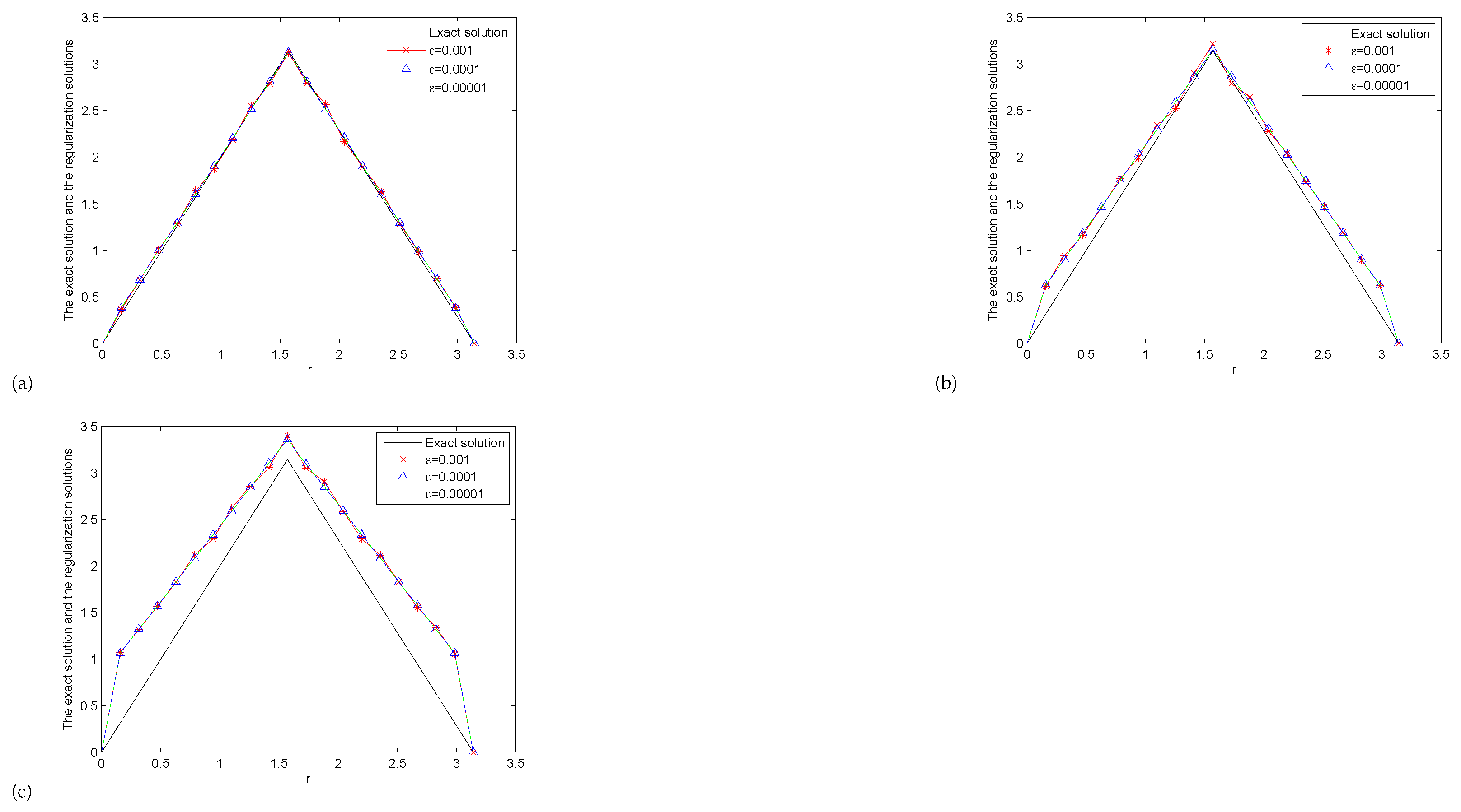
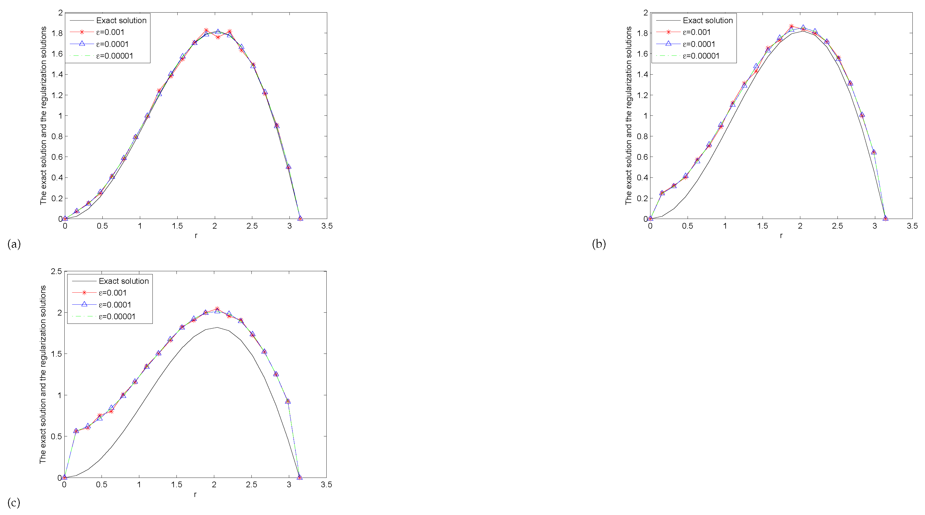
Figure 1 presents the comparison between the Landweber iterative regularization solution ${\psi }^{N,\delta }\left(r\right)$ and the exact solution $\psi \left(r\right)$ in Example 1. Figure 2 presents the comparison between the Landweber iterative regularization solution ${\psi }^{N,\delta }\left(r\right)$ and the exact solution $\psi \left(r\right)$ in Example 2. From Figure 1 and Figure 2, firstly, we can see that the smaller $\epsilon$ and $\alpha$, the better the fitting effect. Secondly, we find that the numerical results are very sensitive to the fractional order $\alpha$. When $\alpha$ is very small, the calculation results are very good, but once $\alpha$ is slightly larger, the calculation results are very bad. It shows that the ill-posed problem is mainly reflected by $\alpha$. Thirdly, we can also find that the numerical results are not particularly sensitive to the disturbance error $\epsilon$. When $\epsilon$ is small, the calculation results are good. As the disturbance error $\epsilon$ becomes larger, the calculation results are not as good as when the disturbance error $\epsilon$ is small, but the change is not great. Fourth, we can find that the numerical effect of Example 1 is slightly better than that of Example 2, which indicates that the inversion effect for functions with good properties is better than that for functions with poor properties.

Figure 1. The comparison between the regularization solutions and the exact solution for Example 1: (a) $\alpha =0.05$, (b) $\alpha =0.15$, (c) $\alpha =0.25$.

Figure 2. The comparison between the regularization solutions and the exact solution for Example 2: (a) $\alpha =0.05$, (b) $\alpha =0.15$, (c) $\alpha =0.25$.

Secondly, in order to check the calculation results for different time and space steps, we use Example 1 to compute the relative error between the exact solution and the regularization solution. We choose $\alpha =0.15$, $\epsilon =0.001$, $p=2$. From Table 1 and Table 2, we can see that the relative error of numerical results gradually increases with the increase of K after taking $m=10$. At the same time, the relative error of numerical results gradually increases with the increase of m after taking $K=10$. However, the relative error of the numerical results does not increase rapidly with the increase of the values of m and K, so in the previous numerical experiments, we took $m=10,K=15.$

Table 1. The relative error between the exact solution and the regularization solution for $M=10$.

K	5	10	15	20	25	30	35
Relative error	0.1968	0.0993	0.1326	0.1433	0.1665	0.1602	0.1772

Table 2. The relative error between the exact solution and the regularization solution for $K=10$.

M	5	10	15	20	25	30	35
Relative error	0.1602	0.0993	0.2822	0.4498	0.5678	0.6043	0.7543

7. Conclusions

In this manuscript, the initial value problem of time-fractional diffusion equation in an axisymmetric domain is considered. The Landweber iterative regularization method is used to solve this problem. Moreover, under the a priori and a posteriori regularization parameter choice rules, the error estimates are all obtained. Through different kind of examples, the Landweber iterative regularization method’s effectiveness for this problem is presented.

References

- Young, D.L.; Tsai, C.C.; Murugesan, K.; Fan, C.M.; Chen, C.W. Time-dependent fundamental solutions for homogeneous diffusion problems. Eng. Anal. Bound. Elem. 2004, 28, 1463–1473. [Google Scholar] [CrossRef]
- Alcouffe, R.E.; Brandt, A.; Dendy, J.E.; Painter, J.W. The multi-grid method for the diffusion equation with strongly discontinuous coefficients. SIAM J. Sci. Comput. 1981, 2, 430–454. [Google Scholar] [CrossRef]
- Luchko, Y. Initial-boundary-value problems for the one-dimensional time-fractional diffusion equation. Fract. Calc. Appl. Anal. 2012, 15, 141–160. [Google Scholar] [CrossRef]
- Kemppainen, J. Existence and uniqueness of the solution for a time-fractional diffusion equation. Fract. Calc. Appl. Anal. 2011, 14, 411–417. [Google Scholar] [CrossRef]
- Wei, T.; Zhang, Y. The backward problem for a time-fractional diffusion-wave equation in a bounded domain. Comput. Math. Appl. 2018, 75, 3632–3648. [Google Scholar] [CrossRef]
- Tuan, N.H.; Long, L.D.; Tatar, S. Tikhonov regularization method for a backward problem for the inhomogeneous time-fractional diffusion equation. Appl. Anal. 2018, 97, 842–863. [Google Scholar] [CrossRef]
- Liu, J.J.; Yamamoto, M. A backward problem for the time-fractional diffusion equation. Appl. Anal. 2010, 89, 1769–1788. [Google Scholar] [CrossRef]
- Yang, F.; Wu, H.H.; Li, X.X. Three regularization methods for identifying the initial value of time fractional advection-dispersion equation. Comput. Appl. Math. 2022, 41, 60. [Google Scholar] [CrossRef]
- Wei, T.; Wang, J.G. A modified quasi-boundary value method for an inverse source problem of the time-fractional diffusion equation. Appl. Numer. Math. 2014, 78, 95–111. [Google Scholar] [CrossRef]
- Wei, T.; Zhang, Z.Q. Reconstruction of a time-dependent source term ina time-fractional diffusion equation. Eng. Anal. Bound. Elem. 2013, 37, 23–31. [Google Scholar] [CrossRef]
- Luc, N.H.; Baleanu, D.; Agarwal, R.P. Identifying the source function for time fractional diffusion with non-local in time conditions. Comput. Appl. Math. 2021, 40, 1–21. [Google Scholar] [CrossRef]
- Ozbilge, E.; Demir, A. Inverse problem for a time-fractional parabolic equation. J. Inequal. Appl. 2015, 2015, 81. [Google Scholar] [CrossRef]
- Li, G.; Zhang, D.; Jia, X.; Yamamoto, M. Simultaneous inversion for the space-dependent diffusion coefficient and the fractional order in the time-fractional diffusion equation. Inverse Probl. 2013, 29, 065014. [Google Scholar] [CrossRef]
- Cheng, W.; Fu, C.L.; Qian, Z. A modified Tikhonov regularization method for a spherically symmetric three-dimensional inverse heat conduction problem. Math. Comput. Simulat. 2007, 75, 97–112. [Google Scholar] [CrossRef]
- Cheng, W.; Fu, C.L.; Qian, Z. Two regularization methods for a spherically symmetric inverse heat conduction problem. Appl. Math. Model. 2008, 32, 432–442. [Google Scholar] [CrossRef]
- Cheng, W.; Ma, Y.J. A modified quasi-boundary value method for solving the radially symmetric inverse heat conduction problem. Appl. Anal. 2016, 96, 1–11. [Google Scholar] [CrossRef]
- Cheng, W. Stability estimate and regularization for a radially symmetric inverse heat conduction problem. Bound. Value Probl. 2017, 2017, 53. [Google Scholar] [CrossRef]
- Yu, J.N.; Luo, G.W.; Deng, Z.C. Numerical identification of source terms for a two dimensional heat conduction problem in polar coordinate system. Appl. Math. Model. 2013, 37, 939–957. [Google Scholar]
- Xiong, X.T.; Ma, X.J. A Backward Identifying Problem for an Axis-Symmetric Fractional Diffusion Equation. Math. Model. Anal. 2017, 22, 311–320. [Google Scholar] [CrossRef]
- Djerrar, I.; Alem, L.; Chorfi, L. Regularization method for the radially symmetric inverse heat conduction problem. Bound. Value Probl. 2017, 2017, 159. [Google Scholar] [CrossRef]
- Yang, F.; Ren, Y.P.; Li, X.X. Landweber iteration regularization method for identifying unknown source on a columnar symmetric domain. Inverse Probl. Sci. Eng. 2018, 26, 1109–1129. [Google Scholar] [CrossRef]
- Yang, F.; Zhang, P.; Li, X.X.; Ma, X.Y. Tikhonov regularization method for identifying the space-dependent source for time-fractional diffusion equation on a columnar symmetric domain. Adv. Differ. Equ. 2020, 2020, 128. [Google Scholar] [CrossRef]
- Yang, F.; Wang, N.; Li, X.X. Landweber iterative method for an inverse source problem of time-fractional diffusion-wave equation on spherically symmetric domain. J. Appl. Anal. Comput. 2020, 10, 514–529. [Google Scholar] [CrossRef] [PubMed]
- Podlubny, I. Fractional Differential Equation; Academic Press: San Diego, CA, USA, 1999. [Google Scholar]
- Bakushinsky, A.B.; Kokurin, M.Y. Iterative Methods for Approximate Solution of Inverse Problems; Springer: New York, NY, USA, 2004. [Google Scholar]
- Beilina, L.; Klibanov, M. Approximate Global Convergence and Adaptivity for Coefficient Inverse Problems; Springer: Berlin/Heidelberg, Germany, 2012. [Google Scholar]
- Ito, K.; Jin, B. Inverse Problems: Tikhonov Theory and Algorithms; Series on Applied Mathematics; World Scientific: Danvers, MA, USA, 2015. [Google Scholar]
- Tikhonov, A.N.; Goncharsky, A.; Stepanov, V.V.; Yagola, A.G. Numerical Methods for the Solution of Ill-Posed Problems; Springer: Berlin/Heidelberg, Germany, 1995. [Google Scholar]
- Engl, H.W.; Hanke, M.; Neubauer, A. Regularization of Inverse Problems; Kluwer Academic Publishes: Boston, MA, USA, 1996. [Google Scholar]
Publisher’s Note: MDPI stays neutral with regard to jurisdictional claims in published maps and institutional affiliations. |
© 2022 by the authors. Licensee MDPI, Basel, Switzerland. This article is an open access article distributed under the terms and conditions of the Creative Commons Attribution (CC BY) license (https://creativecommons.org/licenses/by/4.0/).