A Machine Learning Strategy for the Quantitative Analysis of the Global Warming Impact on Marine Ecosystems

Abstract

It is generally observed that aquatic organisms have symmetric abilities to produce oxygen $\left(O_2\right)$ and fix carbon dioxide $\left(C{O}_2\right)$. A simulation model with time-dependent parameters was recently proposed to better understand the symmetric effects of accelerated climate change on coastal ecosystems. Changes in environmental elements and marine life are two examples of variables that are expected to change over time symmetrically. The sustainability of each equilibrium point is examined in addition to proving the existence and accuracy of the proposed model. To support the conclusions of this research compared to other studies, numerical simulations of the proposed model and a case study are investigated. This paper proposes an integrated bibliographical analysis of artificial neural networks (ANNs) using the Reverse-Propagation with Levenberg–Marquaradt Scheme (RP-LMS) to evaluate the main properties and applications of ANNs. The results obtained by RP-LMS show how to prevent global warming by improving the management of marine fish resources. The reference dataset for greenhouse gas emissions, environmental temperature, aquatic population, and fisheries population (GAPF) is obtained by varying parameters in the numerical Adam approach for different scenarios. The accuracy of the proposed RP-LMS neural network is demonstrated using mean square error (MSE), regression plots, and best-fit output. According to RP-LMS, the current scenario of rapid global warming will continue unabated over the next 50 years, damaging marine ecosystems, particularly fish stocks.

1. Introduction

The struggle between living organisms and their environment is a universal phenomenon. Since the agricultural revolution, emissions of greenhouse gases into the atmosphere have increased rapidly [1,2,3]. The global climate is constantly changing as the concentration of greenhouse gases increases. They mostly affect marine ecosystems as a result of acidification, warming, and natural disasters (floods, tsunamis, and so on) [4,5,6,7,8,9,10,11,12]. The release of extreme greenhouse gases has serious irreversible consequences in the form of climate change and rising temperatures. According to scientists, around $83\%$ of greenhouse gases are produced, and climate change is primarily caused by human activity. Extreme global warming concentrations are causing a rapid rise in sea levels. The average ($C{O}_2$) concentration continued to rise, from 280.01 to 380.01 (ppmv). Examine the last 0.8 million years of history.

Aquatic organisms are speculated to be the most important oxygen ($O_2$) producers and carbon dioxide ($C{O}_2$) absorbers. Through the transportation of energy, high temperatures, and nutrients, marine ecosystems play an important role in balancing ecological change. For example, marine ecosystems act as carbon dioxide sinks, which actually reduces the rate of global warming. Climate change, which is a source of $O_2$ since phytoplankton produces nearly $70\%$ of $O_2$ [13,14], is also a source of proteins and vitamins for humans [15,16,17]. In general, rapid global warming has a negative effect on the number of greenhouse gases in the atmosphere. This makes it harder for marine phytoplankton, fish, and algae to grow [5,6,7]. Numerous studies have been published on the consequences of global climate change on the biodiversity of coastal and marine habitats [18,19,20,21].

Moreover, numerous studies [22,23,24] provide statistical explanations for the probable consequences of climate change on marine coastal biodiversity. A companion article estimates the effects of climate change on a specific coastal area using mathematical approaches. Hiners et al. [25] developed an accurate model to investigate the effects of global climate change on marine aquatic plants and discovered that the rate of evolution of marine plankton differs from that of climate change. Schercher and Petrovski [13] investigated the impact of saturation ($C{O}_2$) on maritime trophic evolution and concluded that it is faster compared to the oceans ($C{O}_2$). Speers et al. [8] demonstrated how degradation and climate change damage aquatic marine biodiversity, particularly coral reefs and fish habitats. Through statistical analysis, they found that almost 92 percent of marine sea creatures may be gone by the end of the year 2100. However, those studies do not specify how or how much the density of marine species will vary as a result of any environmental change. The authors of that research established mathematically and empirically that the consequences of global warming continue to harm entire ecosystems, and that if this scenario continues, 80–90 percent of the diversity of ecological systems could be lost by the end of this century. The effects of climate change on the coastal habitats of the Pacific Ocean were scientifically examined by Asch et al. [10]. The most current analysis distinguishes each of these contributions as a component of the marine ecosystem, and Table 1 makes this distinction quite evident. A set of nonlinear ordinary differential Equation (1) serves as the foundation for the model. The reference dataset for greenhouse gas emissions, environmental temperature, aquatic population, and fisheries population (GAPF) is obtained by modifying the parameters of the NDSolve techniques for various scenarios. Using Equation (1) from 0 to 50 intervals with a 0.04 step size, a reference dataset of 1251 points is generated for each GAPF model scenario.

Table 1. Previous studies compared to this study.

Literature	Parameter Growth Rate of		Effect of Climate Change			Solution		Case
Review	Growth and Rate of Decline		on Marine Ecosystem			Type		Study
	Secondary	Measured	Global Warming	Marine Plankton	Fish Community	Exact	Heuristic
Hinners et al. [25]	Yes	No	Yes	Yes	No	Yes	No	No
Asch et al. [10]	Yes	No	Yes	Yes	Yes	No	No	No
Mandal et al. [16]	No	Yes	Yes	Yes	No	Yes	No	No
Speers et al. [8]	Yes	No	Yes	Yes	Yes	Yes	No	No
Sekerci and	No	Yes	Yes	Yes	No	Yes	No	No
Petrovskii [13]
This study	No	Yes	Yes	Yes	Yes	Yes	Yes	Yes

The GAPF model has previously been studied using various analytical methods; however, the stochastic mathematical processing tool dealing with RP-LMS has recently been used to analyze GAPF. Due to their successful applications in numerous technical and scientific fields, such as sustainable-security assessment [26] digital logic [27], image recognition [28], electronic systems [29], computational intelligence [30], and analog thinking [31], to name just a few, artificial neural networks (ANNs) have emerged as an innovative alternative to mimic systems. Fluid Mechanics [32,33,34,35,36,37], Biomedicine [38,39,40], Financial and Business Systems [41,42], Engineering Application [43], Physics of Fluids [43], Models of Panto-Graph Delay Differential Systems [44], and other interesting ones. Research papers have all benefited from the accurate results provided by stochastic numerical calculations. All these motivating features encourage researchers to use an AI algorithm-based numerical computational model for the numerical exploration model, combining graphical and numerical analysis to predict the future of the coastal environment (algae and freshwater bodies) in the face of the rapid investigation of global warming. The research is divided into many steps, which are summarized below.

• The RP-LMS neural network is a novel supervised computational paradigm that we designed. It is fast and efficient and requires little computing power.
• For the GAPF model, the original mathematical equations are solved by the RK4 method to prepare the dataset for the RP-LMS neural network. For the convenience of readers, the notations used in this paper are summarized in the abbreviation section.
• The presentation of the designed neural network through RP-LMS for successfully resolving the GAPF model was further validated by mean square error, regression analysis, and histogram convergence plot.
• The correctness and repeatability of the design schemes were further validated using reliability, effectiveness, MSE convergence analysis, correlation analysis, and bar charts.
• Table 1 gives a quick summary of some relevant studies conducted in the past and illustrates how they differ from the suggested approach (RP-LMS).

2. Mathematical Formulation

The study aims to find out how global warming affects aquatic ecosystems. Due to the rapid emission of greenhouse gases (plankton and fish community), marine habitats are evaluated in the context of global warming. Environmental phenomena are identified using mathematical models. Heterogeneous processes are divided into four categories, the number of greenhouse gases released into the atmosphere W(t) originating from different (but comparable) sources (slow human activity and natural phenomena) [1], an increase in atmospheric temperature X(t), which leads to a high concentration of carbon dioxide in the environment and is responsible for the greenhouse effect Y(t), and fish density in marine ecosystems decreases with altitude due to rapid temperature rise, salinity, oxygen starvation, and plankton population depletion Z(t). Figure 1 shows a schematic diagram of the model showing how anthropogenic climate change and greenhouse gas concentrations affect ocean life. The following mathematical model, which is made up of a series of NODEs, was recently proposed:

$$\left\{\begin{array}{c}\frac{dW}{dt}=n_{1}W+{\Delta }_{1}ZW-{\Delta }_{2}YW-{\Delta }_{3}X,\hfill \\ \frac{dX}{dt}=n_{2}X+{\psi }_{1}WX-{\psi }_{2}YX,\hfill \\ \frac{dY}{dt}=n_{3}Y(1-\frac{Y}{A_1})+{\chi }_{1}Y-{\chi }_{2}YX-{\chi }_{3}ZY-{\chi }_{4}WY,\hfill \\ \frac{dZ}{dt}=n_{4}Z(1-\frac{Z}{A_2})+{\beta }_{1}YZ-\frac{{\beta }_{2}Z}{\alpha +W}-{\beta }_{3}XZ.\hfill \end{array}\right.$$

(1)

with initial conditions

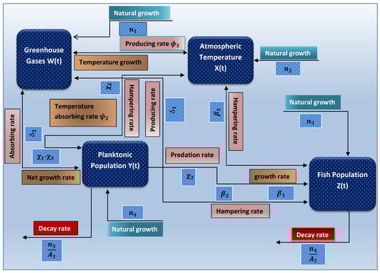
Figure 1. Schematic diagram of Model (1) showing the effect of greenhouse gas on temperature rise and the effect on marine environment and fishing community [16].

• $W_0=W\left(0\right)>0$, $X_0=X\left(0\right)>0$,
• $Y_0=Y\left(0\right)\ge 0$, $Z_0=Z\left(0\right)\ge 0$.

Four different categories are depicted in Figure 1.

• Greenhouse gases that contribute to global warming W(t)
• Atmospheric temperature X(t)
• Planktonic individuals Y(t)
• The Fishing Community Z(t).

The rates at which different factors (mostly human activities and, over time, physical processes) change the number of greenhouse gases released into the atmosphere are represented by Z(t) and W(t). X(t) is the high ambient temperature, which rises steadily with the maximum absorption of ecological GHGs and causes global warming. Y(t) is the strength of the planktonic community in the coastal environment, which is constantly threatened by the effects of climate change. In the presence of UV radiation, environmental gases undergo several chemical reactions. During the reaction phase, they give off energy, which raises the temperature of the environment and makes a number of new GHG components that add to the amount of GHGs in the atmosphere. Here, $n_1$ and $n_2$ represent typical growth rates, respectively. Alternatively, $n_3$ and $n_4$ are the typical growth rates of Y(t) and Z(t) in the absence of negative effects from GHGs and climate change. In maritime zones, Plankton (phytoplankton) absorbs carbon dioxide for respiration, and reducing the number of greenhouse gases in the air. ${\varphi }_1$ represents the rise in GHG intensity caused by the marine fish, while ${\varphi }_2$ represents the planktonic population’s absorption of ambient GHGs whereas ${\varphi }_3$ represents the emission of greenhouse gases as a result of global warming.

The environmental temperature increases accordingly to the quantity of ambient GHGs, such as ${\Delta }_1$, which represents the rise in atmospheric temperature caused by the increase in GHGs. Temperature is a crucial component in marine plankton photosynthesis (phytoplankton). Thus, through photosynthesis, the quantity of maritime phytoplankton population can moderate the temperature rise. Here, ${\Delta }_2$ represents the ambient temperature absorbed by the planktonic population. We consider $A_1$ and $A_2$ to be the sustaining capabilities of the prokaryotes and fishery communities, respectively, with the associated decay rates $\frac{n_3}{A_1}$ and $\frac{n_4}{A_2}$. Although the density of dispersed CO₂ promotes the concentration of maritime phytoplankton, when the density of dissolved CO₂ is so high, it limits phytoplankton metabolism by lowering the volume of dissolved O₂, which slows the growth of the aquatic community. The influence of saturated carbon dioxide and dissolved oxygen deficit limit the growth of marine fisheries. As a result, $chi1$ denotes the rise in planktonic inhabitants brought on by $C{O}_2$ absorption, $ch{i}_2$ reflects the decline in planktonic inhabitants brought on by warming, $ch{i}_3$ represents the improvement in planktonic inhabitants brought on by exploitation or expenditure of fishery resources, and $ch{i}_4$ denotes the reduction in planktonic inhabitants brought on by acidity. While ${\beta }_1$ represents the number of fish that rise as a result of eating plankton, ${\beta }_2$ represents the number of fish that decrease amount of absorbed $C{O}_2$, and ${\beta }_3$ represents the number of fish that decrease due to climate change. Table 2 summarises the parametric descriptions as well as the related values.

Table 2. Describe the relevant values of the parameters used in this study.

Symbols	Descriptions	Values
$n_1$	GHG levels in the oceans are naturally growing.	0.00095 kg/km${}^2$
$n_2$	Plankton-feeding fish growth during the period	0.099 ${}^{\circ }$C
$n_3$	The normal rate of expansion of the aquatic species	0.00225 km${}^{-3}$
$n_4$	The perfectly natural increase in the population of fish	0.0002/1000
${\Delta }_1$	The oceanic aquatic demographic’s rate of GHG production	0.0029 kg/km${}^2$
${\Delta }_2$	GHG absorption rate by planktonic populations in the oceans	0.00099 kg/km${}^2$
${\Delta }_3$	Due to rising temperatures, the rate at which GHGs are emitted	1.0 $\mathsf{\mu }$ kg/km${}^2$
${\chi }_1$	Planktonic population growth rate due to $C{O}_2$	0.00108 km${}^{-3}$
${\chi }_2$	Nutrient rates are slowing as a result of global warming	0.00001 km${}^{-3}$
${\chi }_3$	The rate at which fish consume plankton.	0.0031 km${}^{-3}$
${\chi }_4$	Effects of acidity on plankton loss	10.1 $\mathsf{\mu }$ km${}^{-3}$
${\psi }_1$	GHG-induced increase in the rate of surface temperatures	0.00025 ${}^{\circ }$C
${\psi }_2$	Rate of temperature absorption by the planktonic community	0.00565 ${}^{\circ }$C
${\beta }_1$	Plankton feeding/consumption increases the growth rate of fish populations.	$175\mathsf{\mu }$/1000
${\beta }_2$	The fish population declines to owe to acidification caused by GHGs.	$190\mathsf{\mu }$/1000
${\beta }_3$	Global warming is slowing the growth of fish populations	$61\mathsf{\mu }$/1000
$\alpha$	Stability in the level of saturation	0.01
$A_1$	Planktonic population’s capacity for sustained growth	1,000,000 km
$A_2$	The population’s ability to sustain themselves	10,000 km

The (GAPT) model is discussed for three different scenarios by considering the parameters such as the absorption rate of greenhouse gases by the plankton population in oceans (${\Delta }_1$), inhibition rate of plankton as a consequence of climate change (${\Delta }_2$) and global climate change has a significant impact on fish populations (${\Delta }_3$). The variation of different parameters is clearly discussed in Table 3.

Table 3. Variation of the parameters in the case study.

Scenarios	Cases	Parameters
		${\Delta }_{\mathbf{1}}$	${\Delta }_{\mathbf{2}}$	${\Delta }_{\mathbf{3}}$	${\mathbf{\chi }}_{\mathbf{1}}$	${\mathbf{\chi }}_{\mathbf{2}}$	${\mathbf{\chi }}_{\mathbf{3}}$	${\mathbf{\chi }}_{\mathbf{4}}$	${\mathbf{\beta }}_{\mathbf{1}}$	${\mathbf{\beta }}_{\mathbf{2}}$	${\mathbf{\beta }}_{\mathbf{3}}$	$\mathbf{\alpha }$	${\mathbf{\psi }}_{\mathbf{1}}$	${\mathbf{\psi }}_{\mathbf{2}}$
1	1	0.0029	0.00101	1	0.0011	0.00001	0.0031	10.1	0.000000175	0.00000019	6.1 $\times {10}^{-7}$	0.01	0.00025	0.00565
	2	0.0029	0.00108	1	0.0011	0.00001	0.0031	10.1	0.000000175	0.00000019	6.1 $\times {10}^{-7}$	0.01	0.00025	0.00565
	3	0.0029	0.00114	1	0.0011	0.00001	0.0031	10.1	0.000000175	0.00000019	6.1 $\times {10}^{-7}$	0.01	0.00025	0.00565
2	1	0.0029	0.00099	1	0.0011	0.00001	0.0031	10.1	0.000000175	0.00000019	6.1 $\times {10}^{-7}$	0.01	0.00025	0.00565
	2	0.0029	0.00099	1	0.00114	0.00001	0.0031	10.1	0.000000175	0.00000019	6.1 $\times {10}^{-7}$	0.01	0.00025	0.00565
	3	0.0029	0.00099	1	0.00118	0.00001	0.0031	10.1	0.000000175	0.00000019	6.1 $\times {10}^{-7}$	0.01	0.00025	0.00565
3	1	0.0029	0.00099	1	0.0011	0.00001	0.0031	10.1	0.000000175	0.00000019	0.000061	0.01	0.00025	0.00565
	2	0.0029	0.00099	1	0.0011	0.00001	0.0031	10.1	0.000000175	0.00000019	0.00071	0.01	0.00025	0.00565
	3	0.0029	0.00099	1	0.0011	0.00001	0.0031	10.1	0.000000175	0.00000019	0.001361	0.01	0.00025	0.00565

3. Design Methodology

Predicting outcomes from datasets with labeled results is the goal of supervised machine learning, which is an area of artificial intelligence that describes a set of techniques and concepts for doing so. A powerful teaching technique that can be used to learn the method is an artificial neural network, which uses optimization to minimize error functions [45,46]. The network operating system is divided into two parts. The first part discusses the basic foundations of the RP-LMS dataset design, while the second part describes how to implement RP-LMS in the real world. Here, RP-LMS is used to numerically analyze the GAPF paradigm introduced by Equation (1). The suggested RP-LMS is introduced for multiple scenarios, with S-1 representing no change in fish numbers, S-2 showing an increase in planktonic populations due to increased $C{O}_2$ uptake, and S-3 showing a drop in fish numbers as a result of global warming. For the RP-LMS, the reference dataset is created using the Runge–Kutta technique and the NDSolver in Mathematica. For each variable with a range from 0 to 50, we provide 1251 discrete data points by maintaining a step size of 0.04. The collected information is then divided into three different datasets: one dataset is used for training (weight adjustment), one for validation (managing the learning process), and one for testing (evaluating the accuracy of the approximation). There is a predetermined number of observations in each dataset from which to calculate the optimal convergence rate.

To train the networks, the input vectors and target vectors have been arbitrarily split into three sets: $70\%$ of the total dataset was used for training, $15\%$ of the dataset was used to determine whether the network was generalizing and to halt training before the model became overfit, and $15\%$ of the dataset was used to test the generalization of the network in a manner that was completely independent of the training. The number of layers, number of hidden neurons, learning process, and activation function employed in the experiment are all elaborated in the Table 4. Activation functions are the most important component of any deep learning neural network; they are primarily used to decide the outcome of deep learning techniques, their correctness, and the effectiveness of the training phase that can create or split a large-scale neural network. They determine whether to access or depress neurons in order to achieve the expected output depicted Figure 2. Since the neural network is sometimes trained with millions of data points, the activation function must be efficient and should reduce the time it takes to do a computation. The activation function used in this study is sigmoid function also called logistic function and can be calculated by

$$\sigma \left(\zeta \right)=\frac{1}{1+e^{-z}}$$

(2)

where z is a real number and the number of nodes in a neural network hidden layer is calculated by

$$N=round(\frac{2\times iN}{3}+oN),$$

(3)

where $iN$ represents the number of input nodes and $oN$ represents the number of output nodes. Additionally, as activation functions differ from one another, it is simple to apply back propagations and optimum techniques when measuring gradient loss functions in neural networks.

Table 4. The dimensions and structure of the experiment’s parameters.

Index	Description
Number of layers	Three
Layers structure	One input, one hidden, and one output layer
Hidden neurons	20–80
Training samples	875 samples
Testing samples	188 samples
Validation samples	188 sample
Learning methodology	Levenberg–Marquaradt Scheme
Label target data	Created with Adams numerical method
Maximum iteration	1000
Activation function	Sigmoid Symmetric Transfer Function

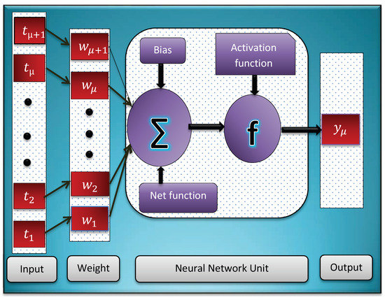
Figure 2. Architecture of artificial neural networks with single neuron.

The architectures of artificial neural networks are shown in Figure 3. The GAPF model is trained multiple times to generate different results due to different initial conditions and samples. The neural network (RP-LMS) requires more memory but less time. Figure 4 shows the detailed flow chart for the design methodology. The mean squared discrepancy between output and objectives is referred to as mean square error. Lower numbers are preferable, while 0 indicates that there is no mistake. Table 4 lists all the important experimental details, such as the total number of layers, the total number of hidden neurons, and the activation function that will be used in the proposed study.

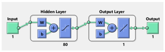
Figure 3. Neural networks architecture.

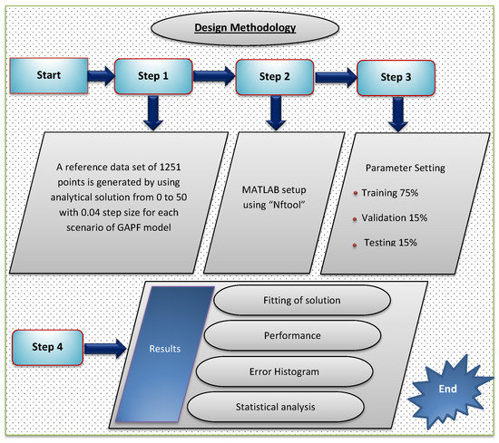
Figure 4. Flow chart for the design methodology.

4. Discussion on Symmetry in Results

This section contains extensive scenario-based simulations, as well as a series of tables and graphs showing the validity and symmetry in the results of the suggested RP-LMS. Various examples of the GAPF model are constructed to evaluate the performance and efficiency of the design algorithm. The variance in different parameters and instances evaluated in the suggested model is shown in Table 5. The absorption ratio of GHGs by aquatic populations in seas (${\Delta }_2$) varies for various situations in the first scenario, while the average growth of the aquatic population (${\chi }_1$) due to $C{O}_2$ varies for three different scenarios in the second scenario. Similarly, the rate of global warming affecting fish populations (${\beta }_3$) varies for different cases of study in Scenario (3). The fourth order Runge–Kutta solver in the MATHEMATICA programmer was used to carry out the numerical simulations of the Model (1). Rk4 obtains the input dataset for (RP-LMS) which ranges from 0 to 50 with a fixed time interval of 0.04. The dataset generates 1251 input points with $15\%$ for validation, $70\%$ for training, and $15\%$ for users to test. The mean square error measures the average squared deviation from the goal value in relation to the outputs. Figure 5 demonstrates the best performance and symmetry for greenhouse gases and ambient temperature for scenario one, and the best validation performance is obtained only at epoch 7, where the values are (5.89 $\times {10}^{-11}$ and 3.97 $\times {10}^{-11}$). On the other hand, Figure 6 demonstrates the best performance for the marine population and the fish community after eight iterations, and the performance obtained for both categories is 1.43 $\times {10}^{-10}$ and 2.40 $\times {10}^{-10}$).

Table 5. Numerical analysis of the RP-LMS in terms of mu, gradient, performance, and number of iterations for Scenarios 1 and 2.

Fitness on MSN
Scenario	Case Index	Neuron Setting	Training	Validation	Testing	Gradient	Performance	Mu	Epochs	R
	w(t)	80	4.67 $\times {10}^{-11}$	5.89 $\times {10}^{-11}$	5.61 $\times {10}^{-11}$	4.36 $\times {10}^{-9}$	5.89 $\times {10}^{-11}$	1.00 $\times {10}^{-10}$	7	1
1	X(t)	80	5.61 $\times {10}^{-11}$	1.43 $\times {10}^{-10}$	2.12 $\times {10}^{-10}$	1.4817 $\times {10}^{-8}$	3.97 $\times {10}^{-11}$	1.00 $\times {10}^{-10}$	7	1
	Y(t)	80	3.11 $\times {10}^{-13}$	3.81 $\times {10}^{-13}$	3.42 $\times {10}^{-13}$	7.91 $\times {10}^{-8}$	1.43 $\times {10}^{-10}$	1.00 $\times {10}^{-12}$	9	1
	Z(t)	80	2.06 $\times {10}^{-11}$	2.10 $\times {10}^{-11}$	1.92 $\times {10}^{-11}$	4.4005 $\times {10}^{-8}$	2.40 $\times {10}^{-10}$	1.00 $\times {10}^{-10}$	7	1
	w(t)	45	4.09 $\times {10}^{-11}$	3.97 $\times {10}^{-11}$	2.45 $\times {10}^{-11}$	9.91 $\times {10}^{-8}$	3.81 $\times {10}^{-13}$	1.00 $\times {10}^{-12}$	234	1
2	X(t)	45	1.24 $\times {10}^{-10}$	2.40 $\times {10}^{-10}$	1.64 $\times {10}^{-10}$	9.98 $\times {10}^{-8}$	1.82 $\times {10}^{-13}$	1.00 $\times {10}^{-12}$	368	1
	Y(t)	45	1.61 $\times {10}^{-13}$	1.82 $\times {10}^{-13}$	1.87 $\times {10}^{-13}$	3.62 $\times {10}^{-7}$	2.10 $\times {10}^{-11}$	1.00 $\times {10}^{-8}$	1000	1
	Z(t)	45	6.29 $\times {10}^{-13}$	3.75 $\times {10}^{-12}$	1.54 $\times {10}^{-12}$	3.73 $\times {10}^{-7}$	3.75 $\times {10}^{-12}$	1.00 $\times {10}^{-12}$	1000	1

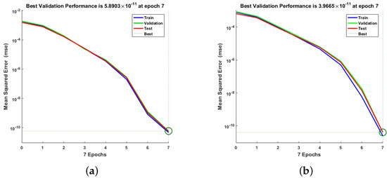
Figure 5. Mean square error of RP-LMS through NNs for greenhouse gases and ambient temperature for Scenario 1. (a) W(t); (b) X(t).

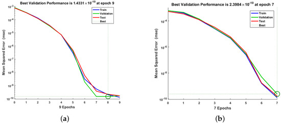
Figure 6. Mean square error of RP-LMS through NNs for aquatic population and fish population for Scenario 1. (a) Y(t), (b) Z(t).

The best performance can be obtained for Scenario 2 by varying the average growth rate of the aquatic population, as shown in Figure 7. The highest performance results for greenhouse gases, atmospheric temperature, marine plankton, and fish community are (3.81 $\times {10}^{-13}$, 1.82 $\times {10}^{-13}$, 2.10 $\times {10}^{-11}$, 3.75 $\times {10}^{-12}$), respectively.

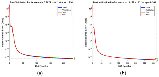
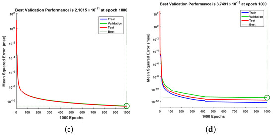
Figure 7. Mean square error of RP-LMS through NNs for greenhouse gases, ambient temperature, aquatic population, and fish population for Scenario 2. (a) W(t), (b) X(t), (c) Y(t), (d) Z(t).

The proposed method has many parameters, such as mu, gradient, and many more. However, mu and gradient are the most well-known parameters. Mu is the part of the algorithm that controls how the neural network is trained. The choice of mu has a direct effect on the convergence of errors. In RP-LMS, mu depends on the maximum eigenvalue of the correlation matrix that was given as input. The default setting for the RP-LMS input value is 0.001, and its range is between 0.8 and 1. The outcomes of the RP-LMS through the supervised neural network for Scenario 1 in terms of mu, gradient, and validation checks for greenhouse gases, ambient temperature, aquatic population, and fish population are presented in Figure 8. By using only 7 to 10 iterations, the values for gradient are 4.36 $\times {10}^{-9}$, 1.49 $\times {10}^{-8}$, 7.91 $\times {10}^{-8}$, 4.405 $\times {10}^{-8}$; mu is 1 $\times {10}^{-10}$, 1 $\times {10}^{-10}$, 1 $\times {10}^{-12}$, 1 $\times {10}^{-10}$. In the same way, Figure 9 and Figure 10 show the gradient and mu values for Scenario 2, which are 9.91 $\times {10}^{-8}$, 9.98 $\times {10}^{-8}$, 3.62 $\times {10}^{-7}$, 3.73 $\times {10}^{-7}$ and 9.91 $\times {10}^{-8}$, 9.98 $\times {10}^{-8}$, 3.62 $\times {10}^{-7}$, 3.73 $\times {10}^{-7}$, respectively, at different numbers of iterations. The number of epochs can vary from 0 to 1000.

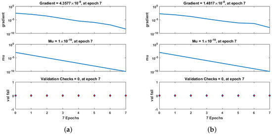
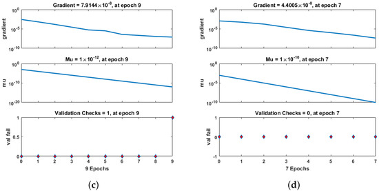
Figure 8. Performance of RP-LMS through SNN in terms of mu, gradient, and validation checks for greenhouse gases, ambient temperature, aquatic population, and fish population for Case 1. (a) W(t), (b) X(t), (c) Y(t), (d) Z(t).

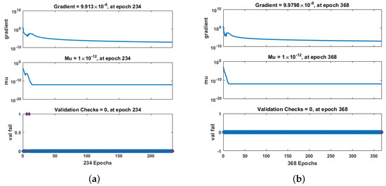
Figure 9. Performance of RP-LMS through SNN in terms of mu, gradient, and validation checks for greenhouse gases and ambient temperature for Case 2. (a) W(t), (b) X(t).

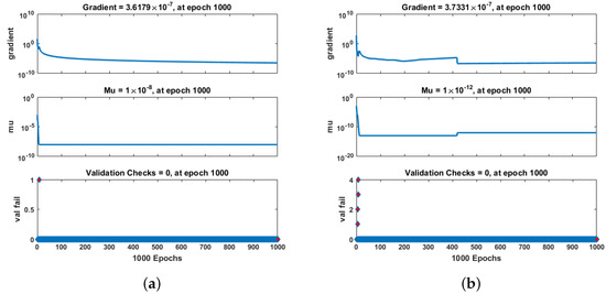
Figure 10. Performance of RP-LMA through SNN in terms of mu, gradient, and validation checks for aquatic population, and fish population for Case 2. (a) Y(t), (b) Z(t).

Figure 11 and Figure 12 show symmetric regression graphs of network outputs in relation to training, validation, and test set targets. The data must fall along a 45 degree line, where the network outputs are equal to the targets, for a perfect match. With R values of 0.95 or higher, the fit is acceptable for all datasets included in this problem. You can retrain the network by clicking Retrain in nftool if you need even more accurate results. This will alter the network’s initial weights and biases, and it is possible that a retrained network will be better for it. In the GAPF model, the regression value is always 1. This shows that the proposed method is very effective. Moreover, for each scenario of the proposed model, we achieved a perfect surrogate model, as depicted on the lift side of Figure 9 and Figure 10; this demonstrates that the methodology is more successful for data-driven real-world situations. Using RP-LMS, we can generate a proxy model for even the largest datasets.

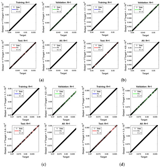
Figure 11. Regression analysis of RP-LMS through SNN for training, validation, testing, and all samples, respectively, for the GAPF model in Case 1. (a) W(t), (b) X(t), (c) Y(t), (d) Z(t).

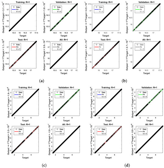
Figure 12. Regression analysis of RP-LMS through SNN for training, validation, testing, and all samples, respectively, for the GAPF model in Case 2. (a) W(t), (b) X(t), (c) Y(t), (d) Z(t).

The graphical analysis of the discussed methodology is further explained statistically in the following tables. Table 5 represents the detailed discussion of the proposed methodology for each scenario, such as the number of hidden neurons and the computation time taken for RP-LMS. Table 5 also shows the number of epochs for the proposed model in each scenario. Furthermore, it also explains the testing, validating, and performance data in each case. The numerical data for mu parameter, gradient, and regression is also discussed in the below table. Figure 13, Figure 14 and Figure 15 shows the error histogram, and fitting graphs provide additional evidence of the effectiveness of the network. The training data is represented by the brown bars in Figure 13, the validation data is represented by the green bars, and the testing data is represented by the red bar. You can use the histogram to find outliers or data points where the fit is much worse than the rest of the data.

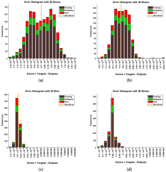
Figure 13. Error histogram for the proposed methodology in terms of greenhouse gases, ambient temperature, aquatic population, and fish population for Case Study 1. (a) W(t), (b) X(t), (c) Y(t), (d) Z(t).

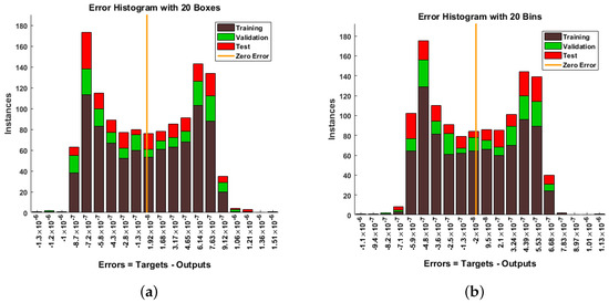
Figure 14. Error histogram for the proposed methodology in terms of greenhouse gases and ambient temperature for Case Study 2. (a) W(t), (b) X(t).

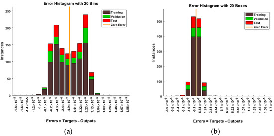
Figure 15. Error histogram for the proposed methodology in terms of aquatic population and fish population for Case Study 2. (a) Y(t), (b) Z(t).

In addition, Figure 16, Figure 17, Figure 18 and Figure 19 show a robust system behavior expected for the differential signaling of greenhouse gases with human plankton. The increase in greenhouse gas emissions is shown in the Figure 16. Figure 17 shows the increase in greenhouse gases due to the number of plankton contributing to the decrease in air temperature, and Figure 18 shows the increase in the population of plankton with increasing atmospheric pressure. On the other hand, as the females consume more plankton, their growth corresponds to the growth of the plankton populations. As plankton concentration increases to support $C{O}_2$ digestion, the number of fish in the total plankton diet increases, total $O_2$ digestion, and sea temperature decrease as shown in Figure 17 and Figure 19. Table 6, Table 7, Table 8 and Table 9 show statistical analysis of numerical solutions of the proposed methodology with the results obtained from a numerically solving model using “NDsolve” by varying a different number of parameters. The discussion also shows the error analysis of the comparative study.

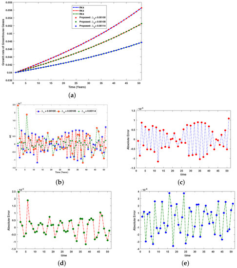
Figure 16. Comparison between the numerical reference solution and the proposed RP-LMS through SNN for greenhouse gases. (a) Impact of ${\Delta }_2$ on greenhouse gases, (b) collective analysis of Absolute Error, (c) analysis of case 1’s errors, (d) analysis of case 2’s errors, (e) analysis of case 3’s errors.

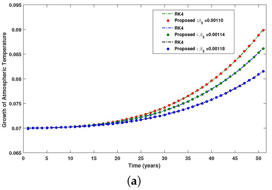
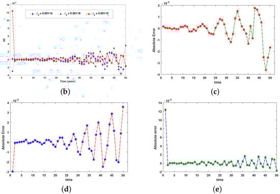
Figure 17. Comparison between the numerical reference solution and the proposed RP-LMS through SNN for ambient temperature. (a) Impact of ${\beta }_3$ on atmospheric temperature, (b) collective analysis of Absolute Error, (c) analysis of case 1’s errors, (d) analysis of case 2’s errors, (e) analysis of case 3’s errors.

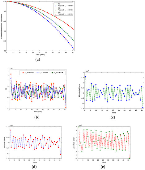
Figure 18. Comparison between the numerical reference solution and the proposed RP-LMS through SNN for aquatic population. (a) Impact of ${\chi }_1$ on planktonic population, (b) collective analysis of Absolute Error, (c) analysis of case 1’s errors, (d) analysis of case 2’s errors, (e) analysis of case 3’s errors.

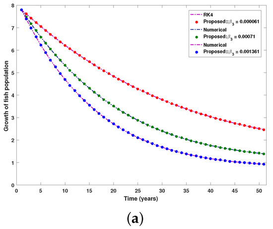
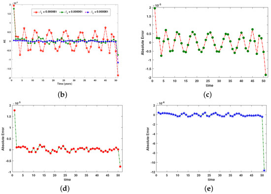
Figure 19. Comparison between the numerical reference solution and the proposed RP-LMS through SNN for fish population. (a) Impact of ${\beta }_3$ on fish population, (b) collective analysis of Absolute Error, (c) analyze of error for case 1, (d) analyze of error for case 2, (e) analyze of error for case 3.

Table 6. Statistical analysis of numerical solution and proposed methodology for varying GHG concentration through aquatic inhabitants in coral reefs, as well as error analysis for Greenhouse Gases.

${\mathsf{\Delta }}_2$ = 0.00101				${\mathsf{\Delta }}_2$ = 0.00108			${\mathsf{\Delta }}_2$ = 0.00114
t	RK4-W(t)	RP-LMS	Absolute Errors	RK4-W(t)	RP-LMS	Absoluten Errors	RK4-W(t)	RP-LMS	Absolute Errors
0	0.04	0.040001	$9.03\times {10}^{-6}$	0.04	0.039975	2.46$\times {10}^{-5}$	0.04	0.04	4.69 $\times {10}^{-6}$
3.96	0.040976	0.040969	6.57 $\times {10}^{-6}$	0.040749	0.040753	$4.19\times {10}^{-6}$	0.040468	0.040467	1.07 $\times {10}^{-6}$
7.96	0.041994	0.041987	6.89 $\times {10}^{-6}$	0.041528	0.04153	$1.04\times {10}^{-6}$	0.040953	0.040954	$1.08\times {10}^{-6}$
11.96	0.043052	0.043048	4.47 $\times {10}^{-6}$	0.042335	0.042332	2.96 $\times {10}^{-6}$	0.041454	0.041455	$4.06\times {10}^{-7}$
15.96	0.044156	0.044153	2.97 $\times {10}^{-6}$	0.043174	0.043173	9.53 $\times {10}^{-7}$	0.041974	0.041972	1.98 $\times {10}^{-6}$
19.96	0.045312	0.045309	3.15 $\times {10}^{-6}$	0.044051	0.044057	$6.90\times {10}^{-6}$	0.042517	0.042518	$6.48\times {10}^{-7}$
23.96	0.04653	0.046531	$1.78\times {10}^{-6}$	0.044971	0.044968	3.16 $\times {10}^{-6}$	0.043086	0.043089	$3.24\times {10}^{-6}$
27.96	0.047816	0.047825	$8.56\times {10}^{-6}$	0.045941	0.045937	4.35 $\times {10}^{-6}$	0.043685	0.043687	$2.29\times {10}^{-6}$
31.96	0.049181	0.049189	$7.98\times {10}^{-6}$	0.046968	0.046978	$9.65\times {10}^{-6}$	0.044318	0.04432	$2.31\times {10}^{-6}$
35.96	0.050633	0.050642	$9.26\times {10}^{-6}$	0.048059	0.048063	$3.67\times {10}^{-6}$	0.044989	0.044988	8.63 $\times {10}^{-7}$
39.96	0.052184	0.052187	$3.20\times {10}^{-6}$	0.049222	0.049216	6.21 $\times {10}^{-6}$	0.045704	0.045706	$1.98\times {10}^{-6}$
43.96	0.053845	0.053845	$5.21\times {10}^{-6}$	0.050465	0.050469	$3.65\times {10}^{-6}$	0.046466	0.046469	$2.71\times {10}^{-6}$
47.96	0.055628	0.055624	4.63 $\times {10}^{-6}$	0.051798	0.051803	$5.63\times {10}^{-6}$	0.047283	0.047284	$1.28\times {10}^{-6}$
50	0.056589	0.056578	1.08 $\times {10}^{-5}$	0.052515	0.052517	$2.28\times {10}^{-6}$	0.047722	0.04772	2.29 $\times {10}^{-6}$

Table 7. Statistical analysis of the numerical solution and the proposed methodology for varying the absorption probability of emission by aquatic inhabitants in seas, as well as the error analysis for ambient temperature, are presented.

${\mathit{\beta }}_3$ = 0.00061				${\mathit{\beta }}_3$ = 0.000711			${\mathit{\beta }}_3$ = 0.001361
t	RK4-X(t)	RP-LMS	Absolute Errors	RK4-X(t)	RP-LMS	Absolute Errors	RK4-X(t)	RP-LMS	Absolute Errors
0	0.07	0.069998	1.61 $\times {10}^{-6}$	0.07	0.07003	$2.96\times {10}^{-5}$	0.07	0.069876	0.000124
3.96	0.070063	0.070064	$6.04\times {10}^{-7}$	0.070061	0.070061	4.44 $\times {10}^{-7}$	0.070059	0.070058	5.92 $\times {10}^{-7}$
7.96	0.070209	0.070208	1.10 $\times {10}^{-6}$	0.070195	0.070196	$7.51\times {10}^{-7}$	0.070177	0.070179	$2.08\times {10}^{-6}$
11.96	0.070483	0.070486	$2.72\times {10}^{-6}$	0.070436	0.070437	$2.28\times {10}^{-7}$	0.070377	0.070378	$1.85\times {10}^{-7}$
15.96	0.070933	0.070932	1.04 $\times {10}^{-6}$	0.070822	0.07082	2.34 $\times {10}^{-6}$	0.070683	0.070679	3.30 $\times {10}^{-6}$
19.96	0.071607	0.071607	$5.90\times {10}^{-8}$	0.071391	0.07139	9.44 $\times {10}^{-7}$	0.071117	0.071117	1.74 $\times {10}^{-7}$
23.96	0.072556	0.072555	3.47 $\times {10}^{-7}$	0.072181	0.072187	$6.64\times {10}^{-6}$	0.071706	0.07171	$4.05\times {10}^{-6}$
27.96	0.073834	0.07383	3.55 $\times {10}^{-6}$	0.073235	0.073232	3.07 $\times {10}^{-6}$	0.072478	0.072476	1.72 $\times {10}^{-6}$
31.96	0.075503	0.075507	$4.80\times {10}^{-6}$	0.074602	0.074593	9.04 $\times {10}^{-6}$	0.073463	0.073458	4.69 $\times {10}^{-6}$
35.96	0.077632	0.077631	1.76 $\times {10}^{-6}$	0.076335	0.076353	$1.77\times {10}^{-5}$	0.074694	0.074698	$4.41\times {10}^{-6}$
39.96	0.080304	0.080302	2.12 $\times {10}^{-6}$	0.078495	0.07852	$2.49\times {10}^{-5}$	0.076209	0.07622	$1.15\times {10}^{-5}$
43.96	0.083614	0.083603	1.17 $\times {10}^{-5}$	0.081153	0.081124	2.88 $\times {10}^{-5}$	0.078051	0.078037	1.37 $\times {10}^{-5}$
47.96	0.087678	0.087703	$2.53\times {10}^{-5}$	0.084393	0.084384	8.98 $\times {10}^{-6}$	0.08027	0.080262	8.05 $\times {10}^{-6}$
50	0.090085	0.089821	0.000264	0.086303	0.086154	0.000149	0.081565	0.081496	6.90 $\times {10}^{-5}$

Table 8. Statistical analysis of numerical solution and proposed methodology for varying aquatic rate of growth due to $C{O}_2$, as well as error analysis for aquatic population.

${\mathit{\chi }}_1$ = 0.00101				${\mathit{\chi }}_1$ = 0.00108			${\mathit{\chi }}_1$ = 0.00114
t	RK4-Y(t)	RP-LMS	Absolute Errors	RK4-Y(t)	RP-LMS	Absolute Errors	RK4-Y(t)	RP-LMS	Absolute Errors
0	17.5	17.5	1.58 $\times {10}^{-6}$	17.5	17.5	1.18 $\times {10}^{-6}$	17.5	17.5	7.79 $\times {10}^{-7}$
3.96	17.46275	17.46275	$6.97\times {10}^{-7}$	17.46603	17.46603	$5.58\times {10}^{-7}$	17.47015	17.47015	$2.35\times {10}^{-7}$
7.96	17.39636	17.39636	$6.79\times {10}^{-7}$	17.40947	17.40947	$3.79\times {10}^{-7}$	17.42596	17.42596	6.43 $\times {10}^{-7}$
11.96	17.30152	17.30152	$3.77\times {10}^{-7}$	17.33074	17.33074	$4.76\times {10}^{-7}$	17.36765	17.36765	5.78 $\times {10}^{-7}$
15.96	17.17871	17.1787	4.00 $\times {10}^{-7}$	17.23002	17.23002	$2.45\times {10}^{-7}$	17.29512	17.29512	$2.48\times {10}^{-7}$
19.96	17.02842	17.02842	4.90 $\times {10}^{-7}$	17.10746	17.10746	6.59 $\times {10}^{-7}$	17.20828	17.20828	2.91 $\times {10}^{-7}$
23.96	16.8512	16.8512	$6.22\times {10}^{-7}$	16.96324	16.96324	$6.17\times {10}^{-7}$	17.10699	17.10699	1.04 $\times {10}^{-7}$
27.96	16.64766	16.64766	5.26 $\times {10}^{-7}$	16.79754	16.79754	$2.25\times {10}^{-7}$	16.9911	16.9911	$4.06\times {10}^{-11}$
31.96	16.41845	16.41845	2.25 $\times {10}^{-7}$	16.61057	16.61056	6.34 $\times {10}^{-7}$	16.86044	16.86044	$4.60\times {10}^{-7}$
35.96	16.16432	16.16432	$7.46\times {10}^{-7}$	16.40255	16.40255	$5.56\times {10}^{-8}$	16.71482	16.71482	3.60 $\times {10}^{-7}$
39.96	15.88609	15.88609	$4.01\times {10}^{-7}$	16.17379	16.17379	$3.62\times {10}^{-7}$	16.55409	16.55409	$5.06\times {10}^{-7}$
43.96	15.5847	15.5847	6.51 $\times {10}^{-8}$	15.92463	15.92463	9.43 $\times {10}^{-8}$	16.37806	16.37806	4.10 $\times {10}^{-7}$
47.96	15.26118	15.26118	$6.81\times {10}^{-7}$	15.6555	15.6555	$4.45\times {10}^{-7}$	16.18659	16.18659	5.13 $\times {10}^{-7}$
50	15.08803	15.08803	$1.39\times {10}^{-6}$	15.51071	15.51071	$1.11\times {10}^{-6}$	16.08296	16.08296	$1.00\times {10}^{-6}$

Table 9. Statistical analysis of numerical solution and the proposed methodology for varying hampering rate of fish populations by global warming and also show the error analysis for fish population.

${\mathit{\beta }}_3$ = 0.00101				${\mathit{\beta }}_3$ = 0.001361			${\mathit{\beta }}_3$ = 0.00071
t	RK4-Z(t)	RP-LMS	Absolute Error	RK4-Z(t)	RP-LMS	Absolute Error	RK4-Z(t)	RP-LMS	Absolute Error
0	7.8	7.79998	1.95 $\times {10}^{-5}$	7.8	7.799982	1.77 $\times {10}^{-5}$	7.8	7.8	4.53 $\times {10}^{-7}$
3.96	6.586341	6.58634	6.31 $\times {10}^{-7}$	6.22928	6.229279	1.41 $\times {10}^{-6}$	7.057025	7.057025	2.74 $\times {10}^{-7}$
7.96	5.553165	5.553169	$4.72\times {10}^{-6}$	4.966141	4.966142	$1.03\times {10}^{-6}$	6.378245	6.378246	$1.05\times {10}^{-7}$
11.96	4.687032	4.687033	$5.13\times {10}^{-7}$	3.967926	3.967924	2.17 $\times {10}^{-6}$	5.765623	5.765623	3.40 $\times {10}^{-7}$
15.96	3.96571	3.965706	3.45 $\times {10}^{-6}$	3.185818	3.185819	$7.15\times {10}^{-7}$	5.214275	5.214275	$8.22\times {10}^{-8}$
19.96	3.369767	3.369771	$4.14\times {10}^{-6}$	2.578881	2.578882	$9.97\times {10}^{-7}$	4.719984	4.719985	$3.02\times {10}^{-7}$
23.96	2.881718	2.881713	4.86 $\times {10}^{-6}$	2.112426	2.112426	3.76 $\times {10}^{-7}$	4.278938	4.278939	$3.05\times {10}^{-7}$
27.96	2.485687	2.485692	$5.11\times {10}^{-6}$	1.757278	1.757278	3.88 $\times {10}^{-7}$	3.887535	3.887535	3.45 $\times {10}^{-9}$
31.96	2.167335	2.167331	4.85 $\times {10}^{-6}$	1.489318	1.489318	7.67 $\times {10}^{-7}$	3.542271	3.542271	5.84 $\times {10}^{-8}$
35.96	1.913895	1.9139	$5.90\times {10}^{-6}$	1.289007	1.289007	2.60 $\times {10}^{-7}$	3.239676	3.239676	4.26 $\times {10}^{-9}$
39.96	1.71418	1.714177	2.61 $\times {10}^{-6}$	1.140805	1.140804	4.41 $\times {10}^{-7}$	2.976299	2.976299	$2.42\times {10}^{-7}$
43.96	1.558555	1.558548	7.45 $\times {10}^{-6}$	1.032519	1.03252	$1.02\times {10}^{-6}$	2.748719	2.74872	$1.76\times {10}^{-7}$
47.96	1.438823	1.438821	2.42 $\times {10}^{-6}$	0.954651	0.95465	9.05 $\times {10}^{-7}$	2.553575	2.553575	$2.23\times {10}^{-7}$
50	1.389308	1.389327	$1.86\times {10}^{-5}$	0.924196	0.924203	$7.54\times {10}^{-6}$	2.465482	2.465494	$1.17\times {10}^{-5}$

5. Conclusions

This paper examined the nonlinear ordinary differential equation with an initial condition related to an environmental management model, where greenhouse gases, environmental temperature, plankton population, and fish population are considered as parameters. To study the environmental management model, a hybridized technique based on reverse propagation through a supervised neural network was designed. The solutions obtained by RP-LMS exhibited better symmetry in terms of results obtained and have taken less time and produced a more accurate result compared to the RK4 numerical technique. In addition, the graphical and statistical approaches confirm the stability and symmetry of the design algorithm. We have used graphical and statistical methods to study how changes in the concentration of greenhouse gases (GHGs) affect aquatic ecosystems and global warming. Furthermore, if current trends continue, aquatic organisms will be transformed into conservation lands within the next fifty years due to the ongoing decline in plankton variability and marine resources. In this work, we solve the real-world challenge associated with the system of nonlinear differential equations. Partial differential equations and fractional order differential equations are two real-world problems that can be tackled with this method in the future. In addition, the scope of artificial neural networks can be easily broadened to address problems in other systems where traditional methods have failed, including quick forest plantations, optimum control schemes, fluid dynamics issues (such as the removal of dyes from water), and many others.

References

- Mandal, S.; Islam, M.S.; Biswas, M.H.A.; Akter, S. A mathematical model applied to investigate the potential impact of global warming on marine ecosystems. Appl. Math. Model. 2022, 101, 19–37. [Google Scholar] [CrossRef]
- Lüthi, D.; Le Floch, M.; Bereiter, B.; Blunier, T.; Barnola, J.M.; Siegenthaler, U.; Raynaud, D.; Jouzel, J.; Fischer, H.; Kawamura, K.; et al. High-resolution carbon dioxide concentration record 650,000–800,000 years before present. Nature 2008, 453, 379–382. [Google Scholar] [CrossRef] [PubMed]
- Change, I.C. The Physical Science Basis; Working Group I Contribution to the Fifth Assessment Report of the Intergovernmental Panel on Climate Change; World Meteorological Organization: Geneva, Switzerland, 2013. [Google Scholar]
- Beardall, J.; Stojkovic, S.; Larsen, S. Living in a high CO2 world: Impacts of global climate change on marine phytoplankton. Plant Ecol. Divers. 2009, 2, 191–205. [Google Scholar] [CrossRef]
- Sherman, E.; Moore, J.K.; Primeau, F.; Tanouye, D. Temperature influence on phytoplankton community growth rates. Glob. Biogeochem. Cycles 2016, 30, 550–559. [Google Scholar] [CrossRef]
- Gomiero, A.; Bellerby, R.; Zeichen, M.M.; Babbini, L.; Viarengo, A. Biological responses of two marine organisms of ecological relevance to on-going ocean acidification and global warming. Environ. Pollut. 2018, 236, 60–70. [Google Scholar] [CrossRef] [PubMed]
- Cooley, S.R.; Bello, B.; Bodansky, D.; Mansell, A.; Merkl, A.; Purvis, N.; Ruffo, S.; Taraska, G.; Zivian, A.; Leonard, G.H. Overlooked ocean strategies to address climate change. Glob. Environ. Change 2019, 59, 101968. [Google Scholar] [CrossRef]
- Speers, A.E.; Besedin, E.Y.; Palardy, J.E.; Moore, C. Impacts of climate change and ocean acidification on coral reef fisheries: An integrated ecological–economic model. Ecol. Econ. 2016, 128, 33–43. [Google Scholar] [CrossRef]
- Roxy, M.K.; Modi, A.; Murtugudde, R.; Valsala, V.; Panickal, S.; Prasanna Kumar, S.; Ravichandran, M.; Vichi, M.; Lévy, M. A reduction in marine primary productivity driven by rapid warming over the tropical Indian Ocean. Geophys. Res. Lett. 2016, 43, 826–833. [Google Scholar] [CrossRef]
- Asch, R.G.; Cheung, W.W.; Reygondeau, G. Future marine ecosystem drivers, biodiversity, and fisheries maximum catch potential in Pacific Island countries and territories under climate change. Mar. Policy 2018, 88, 285–294. [Google Scholar] [CrossRef]
- Ma, S.; Liu, Y.; Li, J.; Fu, C.; Ye, Z.; Sun, P.; Yu, H.; Cheng, J.; Tian, Y. Climate-induced long-term variations in ecosystem structure and atmosphere-ocean-ecosystem processes in the Yellow Sea and East China Sea. Prog. Oceanogr. 2019, 175, 183–197. [Google Scholar] [CrossRef]
- Talloni-Álvarez, N.E.; Sumaila, U.R.; Le Billon, P.; Cheung, W.W. Climate change impact on Canada’s Pacific marine ecosystem: The current state of knowledge. Mar. Policy 2019, 104, 163–176. [Google Scholar] [CrossRef]
- Sekerci, Y.; Petrovskii, S. Mathematical modelling of plankton–oxygen dynamics under the climate change. Bull. Math. Biol. 2015, 77, 2325–2353. [Google Scholar] [CrossRef] [PubMed]
- Rana, T.; Imran, M.A.; Baz, A. A Component Model with Verifiable Composition for the Construction of Emergency Management Systems. Arab. J. Sci. Eng. 2020, 12, 10683–10692. [Google Scholar] [CrossRef]
- Barange, M.; Merino, G.; Blanchard, J.; Scholtens, J.; Harle, J.; Allison, E.; Allen, J.; Holt, J.; Jennings, S. Impacts of climate change on marine ecosystem production in societies dependent on fisheries. Nat. Clim. Change 2014, 4, 211–216. [Google Scholar] [CrossRef]
- Mandal, S.; Islam, M.; Biswas, M.; Ali, H. Modeling the potential impact of climate change on living beings near coastal areas. Model. Earth Syst. Environ. 2021, 7, 1783–1796. [Google Scholar] [CrossRef]
- Le Quéré, C.; Moriarty, R.; Andrew, R.M.; Canadell, J.G.; Sitch, S.; Korsbakken, J.I.; Zeng, N.; Schuster, U.; Schwinger, J.; Tilbrook, B.; et al. Global Carbon Budget 2015. Earth Syst. Sci. Data 2015, 7, 349–396. [Google Scholar] [CrossRef]
- Häder, D.P.; Barnes, P.W. Comparing the impacts of climate change on the responses and linkages between terrestrial and aquatic ecosystems. Sci. Total Environ. 2019, 682, 239–246. [Google Scholar] [CrossRef] [PubMed]
- Baltar, F.; Bayer, B.; Bednarsek, N.; Deppeler, S.; Escribano, R.; Gonzalez, C.E.; Hansman, R.L.; Mishra, R.K.; Moran, M.A.; Repeta, D.J.; et al. Towards integrating evolution, metabolism, and climate change studies of marine ecosystems. Trends Ecol. Evol. 2019, 34, 1022–1033. [Google Scholar] [CrossRef]
- McLean, M.; Mouillot, D.; Lindegren, M.; Engelhard, G.; Villéger, S.; Marchal, P.; Brind’Amour, A.; Auber, A. A climate-driven functional inversion of connected marine ecosystems. Curr. Biol. 2018, 28, 3654–3660. [Google Scholar] [CrossRef]
- Ben-Hasan, A.; Christensen, V. Vulnerability of the marine ecosystem to climate change impacts in the Arabian Gulf—An urgent need for more research. Glob. Ecol. Conserv. 2019, 17, e00556. [Google Scholar] [CrossRef]
- Doney, S.C.; Ruckelshaus, M.; Emmett Duffy, J.; Barry, J.P.; Chan, F.; English, C.A.; Galindo, H.M.; Grebmeier, J.M.; Hollowed, A.B.; Knowlton, N.; et al. Climate change impacts on marine ecosystems. Annu. Rev. Mar. Sci. 2012, 4, 11–37. [Google Scholar] [CrossRef] [PubMed]
- Chapman, E.J.; Byron, C.J.; Lasley-Rasher, R.; Lipsky, C.; Stevens, J.R.; Peters, R. Effects of climate change on coastal ecosystem food webs: Implications for aquaculture. Mar. Environ. Res. 2020, 162, 105103. [Google Scholar] [CrossRef] [PubMed]
- Fabien, M.; Laure, V.; Philippe, V.; Nicolas, B.; Caroline, U.; Pierluigi, C.; Antonio, E.; Follesa, M.C.; Michele, G.; Angélique, J.; et al. Capturing the big picture of Mediterranean marine biodiversity with an end-to-end model of climate and fishing impacts. Prog. Oceanogr. 2019, 178, 102179. [Google Scholar]
- Hinners, J.; Hense, I.; Kremp, A. Modelling phytoplankton adaptation to global warming based on resurrection experiments. Ecol. Model. 2019, 400, 27–33. [Google Scholar] [CrossRef]
- Kumar, R.; Baz, A.; Alhakami, H.; Alhakami, W.; Agrawal, A.; Khan, R.A. A hybrid fuzzy rule-based multi-criteria framework for sustainable-security assessment of web application. Ain Shams Eng. J. 2021, 2, 2227–2240. [Google Scholar] [CrossRef]
- Cao, L. Artificial intelligence in retail: Applications and value creation logics. Int. J. Retail. Distrib. Manag. 2021, 49. [Google Scholar] [CrossRef]
- Tian, Y. Artificial intelligence image recognition method based on convolutional neural network algorithm. IEEE Access 2020, 8, 125731–125744. [Google Scholar] [CrossRef]
- Zhao, S.; Blaabjerg, F.; Wang, H. An overview of artificial intelligence applications for power electronics. IEEE Trans. Power Electron. 2020, 36, 4633–4658. [Google Scholar] [CrossRef]
- Li, H.; Wu, P.; Zeng, N.; Liu, Y.; Alsaadi, F.E. A survey on parameter identification, state estimation and data analytics for lateral flow immunoassay: From systems science perspective. Int. J. Syst. Sci. 2022, 1–21. [Google Scholar] [CrossRef]
- Dohn, N.B.; Kafai, Y.; Mørch, A.; Ragni, M. Survey: Artificial Intelligence, Computational Thinking and Learning. KI-Künstliche Intell. 2022, 36, 5–16. [Google Scholar] [CrossRef]
- Khan, N.A.; Alshammari, F.S.; Romero, C.A.T.; Sulaiman, M. Study of Nonlinear Models of Oscillatory Systems by Applying an Intelligent Computational Technique. Entropy 2021, 23, 1685. [Google Scholar] [CrossRef] [PubMed]
- Khan, N.A.; Alshammari, F.S.; Romero, C.A.T.; Sulaiman, M.; Mirjalili, S. An Optimistic Solver for the Mathematical Model of the Flow of Johnson Segalman Fluid on the Surface of an Infinitely Long Vertical Cylinder. Materials 2021, 14, 7798. [Google Scholar] [CrossRef] [PubMed]
- Khan, N.A.; Ibrahim Khalaf, O.; Andrés Tavera Romero, C.; Sulaiman, M.; Bakar, M.A. Application of Intelligent Paradigm through Neural Networks for Numerical Solution of Multiorder Fractional Differential Equations. Comput. Intell. Neurosci. 2022, 2022, 2710576. [Google Scholar] [CrossRef] [PubMed]
- Khan, N.A.; Sulaiman, M.; Tavera Romero, C.A.; Laouini, G.; Alshammari, F.S. Study of Rolling Motion of Ships in Random Beam Seas with Nonlinear Restoring Moment and Damping Effects Using Neuroevolutionary Technique. Materials 2022, 15, 674. [Google Scholar] [CrossRef] [PubMed]
- Ganie, A.H.; Fazal, F.; Tavera Romero, C.A.; Sulaiman, M. Quantitative Features Analysis of Water Carrying Nanoparticles of Alumina over a Uniform Surface. Nanomaterials 2022, 12, 878. [Google Scholar] [CrossRef] [PubMed]
- Khan, M.F.; Sulaiman, M.; Romero, C.A.T.; Alshammari, F.S. A quantitative study of non-linear convective heat transfer model by novel hybrid heuristic driven neural soft computing. IEEE Access 2022, 10, 34133–34153. [Google Scholar] [CrossRef]
- Rahman, I.U.; Sulaiman, M.; Alarfaj, F.K.; Kumam, P.; Laouini, G. Investigation of Non-Linear MHD Jeffery–Hamel Blood Flow Model Using a Hybrid Metaheuristic Approach. IEEE Access 2021, 9, 163214–163232. [Google Scholar] [CrossRef]
- Fawad Khan, M.; Bonyah, E.; Alshammari, F.S.; Ghufran, S.M.; Sulaiman, M. Modelling and Analysis of Virotherapy of Cancer Using an Efficient Hybrid Soft Computing Procedure. Complexity 2022, 2022, 9660746. [Google Scholar] [CrossRef]
- Baz, A.; Alhakami, H.; Alshareef, E. A framework of computational model for predicting the spread of COVID-19 pandemic in Saudi Arabia. Int. J. Intell. Eng. Syst. 2020, 13, 463–475. [Google Scholar] [CrossRef]
- Bukhari, A.H.; Raja, M.A.Z.; Sulaiman, M.; Islam, S.; Shoaib, M.; Kumam, P. Fractional neuro-sequential ARFIMA-LSTM for financial market forecasting. IEEE Access 2020, 8, 71326–71338. [Google Scholar] [CrossRef]
- Ara, A.; Khan, N.A.; Razzaq, O.A.; Hameed, T.; Raja, M.A.Z. Wavelets optimization method for evaluation of fractional partial differential equations: An application to financial modelling. Adv. Differ. Equ. 2018, 2018, 8. [Google Scholar] [CrossRef]
- Khan, N.A.; Sulaiman, M.; Aljohani, A.J.; Bakar, M.A. Mathematical models of CBSC over wireless channels and their analysis by using the LeNN-WOA-NM algorithm. Eng. Appl. Artif. Intell. 2022, 107, 104537. [Google Scholar] [CrossRef]
- Khan, I.; Raja, M.A.Z.; Shoaib, M.; Kumam, P.; Alrabaiah, H.; Shah, Z.; Islam, S. Design of neural network with Levenberg-Marquardt and Bayesian regularization backpropagation for solving pantograph delay differential equations. IEEE Access 2020, 8, 137918–137933. [Google Scholar] [CrossRef]
- Alghamdi, H.; Alsubait, T.; Alhakami, H.; Baz, A. A review of optimization algorithms for university timetable scheduling. Eng. Technol. Appl. Sci. Res. 2020, 10, 6410–6417. [Google Scholar] [CrossRef]
- Iqbal, A.; Raza, M.S.; Ibrahim, M.; Baz, A.; Alhakami, H.; Saeed, M.A. An Improved Approach for Finding Rough Set Based Dynamic Reducts. IEEE Access 2020, 08, 173008–173023. [Google Scholar] [CrossRef]
Publisher’s Note: MDPI stays neutral with regard to jurisdictional claims in published maps and institutional affiliations. |
© 2022 by the authors. Licensee MDPI, Basel, Switzerland. This article is an open access article distributed under the terms and conditions of the Creative Commons Attribution (CC BY) license (https://creativecommons.org/licenses/by/4.0/).