Fractional Landweber Iterative Regularization Method for Solving the Inverse Problem of Time-Fractional Schrödinger Equation

Abstract

In this paper, we consider the inverse problem for the time-fractional Schrödinger equation. This problem is ill-posed, i.e., the solution (if it exists) does not depend continuously on the data. We use the fractional Landweber iterative regularization method to solve this inverse problem and obtain the regularization solution. Under a priori and a posteriori regularization parameter choices, the error estimates are all obtained, respectively.

1. Introduction

The Schrödinger equation is a second-order partial differential equation that combines the concept of material wave and wave equation. It is a basic assumption of quantum mechanics and its correctness can only be tested by experiments. The Schrödinger equation can be derived by using probability distribution and has the form of diffusion equation in this paper. In quantum mechanics, the state of the system is determined by the wave function, so the wave function has become the main object of quantum mechanics research. What is the probability distribution of the value of the mechanical quantity? How does this distribution change over time? These questions need to be solved by solving the wave function. The number of papers on the theoretical analysis of the inverse problem of Schrödinger equation by regularization method is also limited, and the fractional order method is more advantageous than the integer order method to deal with the inverse problem. The fractional derivative model has a global correlation and overcomes the shortcoming that the classical integer order model is not in good agreement with the experimental results. The Riemann–Liouville fractional derivative and Caputo fractional derivative are both improvements of Grunwald–Letnikov’s definition. The order of differentiation and integration of the two is opposite. The Riemann–Liouville fractional derivative is integration before differentiation, and the Caputo fractional derivative is differentiation before integration. The Caputo fractional derivative is often used in the time derivatives of initial-boundary value problems. In [1], Feynman and Hibbs derive the Schrödinger equation for a quantum mechanical particle by using Gauss probability distribution.

The application of the Schrödinger equation is extremely extensive. It has been studied radially by a large number of researchers, not only in the well-known field of physics but also in the field of ill-posed inverse problems of mathematics. In [2], the Schrödinger equation is studied for free particles of the Caputo time-fractional derivative type and the wave function is proved to be invariant under time reversal. In [3], the mathematical problems in non-relativistic quantum mechanics related to Schrödinger equation are mainly discussed, such as spectral theory of one-dimensional and multi-dimensional Schrödinger operator, scattering theory, and functional integral method. In [4], the author studied an inverse problem of the Schrödinger equation with the Dirichlet boundary-value conditions and initial value conditions in a bounded region with potential depending on time. Derivatives of a subset of normals determine the potential, and the appropriate global Carleman estimate is used as a powerful tool to prove the uniqueness and stability of the inverse problem. In this paper, we consider the following inverse thermal time-fractional Schrödinger equation problem with boundary condition

$$\left\{\begin{array}{cc}i{}_0^c{D}_t^{\alpha }u(x,t)+u_{xx}(x,t)=0,\hfill & x>0,t>0,\hfill \\ u(x,0)=0,\hfill & x\ge 0,\hfill \\ u(1,t)=f(t),\hfill & t\ge 0,\hfill \\ u(x,t){\mid }_{x\to \infty }bounded,\hfill & t>0,\hfill \end{array}\right.$$

(1)

where $i=\sqrt{-1}$ is the imaginary unit and ${}_0^c{D}_t^{\alpha }$ is the Caputo time-fractional derivative of order $\alpha (0<\alpha \le 1)$ defined as

$${}_0^c{D}_t^{\alpha }u(x,t)=\left\{\begin{array}{cccc}\hfill & \frac{1}{\Gamma (1-\alpha )}{\int }_0^t{(t-\tau )}^{-\alpha }{u}_{\tau }(x,\tau )d\tau ,\hfill & \hfill & 0<\alpha <1,\hfill \\ \hfill & u_t(x,t),\hfill & \hfill & \alpha =1,\hfill \end{array}\right.$$

in which $\Gamma (·)$ is the Gamma function.

In problem (1), when $f(t)$ is known, this is an inverse problem. We wish to reconstruct the wave function $u(x,t)(0\le x<1)$ by using the additional condition $u(1,t)=f(t)$ as the measurement data. In practical application, $f(t)$ is obtained by measurement, and there is a slight error between the accurate data and the measured data. Therefore, it is assumed that the exact data function $f(t)\in L^2(R)$ and the measured data function $f^{\delta }(t)\in L^2(R)$ satisfy

$$\parallel f(·)-f^{\delta }(·)\parallel \le \delta ,$$

(2)

where $\parallel ·\parallel$ denotes $L^2(R)$-norm and $\delta >0$ is the noise level.

The fractional-order equation [5] replaces the fractional-order derivative with the integer-order derivative as a generalization of classical integer order differential equation in order to better simulate physical dynamic processes and abnormal diffusion in nature, so it has attracted extensive attention of scientific researchers. For example, in [6], the power-law decay process of the prime number distribution described by the fractional derivative equation model is a typical anomalous diffusion, and its performance is far superior to the prime number theory. The distribution of the Mittag–Leffler function of the fractional derivative diffusion equation is consistent with the distribution of prime numbers. At present, there are roughly two types of fractional derivatives mainly studied, namely the Caputo fractional derivative [7] and Riemann–Liouville fractional derivative [8], of which the Caputo fractional derivative has relatively simple requirements for the initial value and it is relatively easy to calculate. The fractional differential equation is widely used in the field of science and engineering and has achieved fruitful research results due to abundant theoretical knowledge, such as analog control theory [9], fluid mechanics [10], biological sciences, and other directions.

The inverse problem [11] of mathematical physics is an emerging field. Compared with the positive problem, it is generated through mathematical modeling. It can be applied to fields such as medicine, biology, and geology, which brings opportunities for industrial progress and scientific and technological revitalization. In [12], the authors study the inverse problem of tidal potential, that is, the closed equation is constructed on the basis of observing sea level function (free surface height), and an iterative algorithm is given. In [13], the author proves the existence and uniqueness of strong solutions to corresponding positive problems under homogeneous Neumann boundary conditions and considering the identification of time-dependent source terms of multi-dimensional time-fractional diffusion equations from Cauchy data of boundary conditions, which is a classical inverse problem. There are also many scholars who have done related research on the inverse problem of the potential in the Schrödinger equation. In [14], the author considers the inverse problem of the potential of the dynamic Schrödinger equation in the definite interval, recovers the spectral function through the boundary control method, and transforms the problem into a convenient classical problem. In [15], a scheme is derived to eliminate the singularity of particles in the soft-core Coulomb potential commonly used in the one-dimensional Schrödinger equation in momentum space. Through this scheme, the author generalizes two numerical simulation methods for the one-dimensional model in the time-fractional Schrödinger equation in the momentum space. One is to use the expansion of the wave function on the potential-free Hamiltonian eigenstate to prove its validity for the laser parameters in the strong field, and the other is to use the straight-line method or the Crank–Nicolson method for time propagation. In [16], the author studied the Laplace transform of the wave function by means of the integral transformation method and obtained the discrete scheme of the radial Schrödinger equation, which has a limited power growth potential and the generalized nuclear Coulomb attraction potential.

In the research field of mathematical physics equations, most of the inverse problems are ill-posed [17]. The concept of well-posed was first put forward by Hadamard in 1923 for the definite solution of the partial differential equations. On the contrary, it is ill-posed. In order to solve the inverse problem effectively, scholars have successively introduced various effective regularization methods in the long process of research, that is, to find the stable approximate solution of the relevant inverse problem. For example, the Landweber iterative regularization method [18,19], fractional Landweber iterative regularization method [20,21], Fourier regularization method [22,23], improved kernel method [24], quasi-boundary regularization method [25], quasi-inverse regularization method [26], Tikhonov regularization method [27], fractional Tikhonov regularization method [28], regularization methods for quasi-boundary and quasi-inverse mixtures, and so on. In this paper, the fractional Landweber iterative regularization method is used to determine the wave function inversely through the right boundary.

The manuscript is organized as follows. In Section 2, we obtain the exact solution of the ill-posed problem (1) by using Fourier transform and inverse Fourier transform, and then its ill-posedness is analyzed. In Section 3, the preliminary results and optimal error bounds of problem (1) are given, which are the basic theoretical analysis part of this paper. In Section 4, the fractional Landweber iterative regularization method is introduced, and the error estimates at $x\in (0,1)$ and the endpoint $x=0$ are given based on the a priori regularization parameter selection rule and a posteriori regularization parameter selection rule, respectively.

2. The Solution of Problem (1) and Ill-Posed Analysis

In this section, the Fourier transform is first applied to the time variable t, and the solution of Equation (1) in the frequency domain is obtained. Then, the exact solution is obtained by the inverse Fourier transform and its ill-posed analysis is carried out. The specific method is to extend the definition domain of the functions $u(x,t)$ and $f(t)$ with respect to the variable t to the whole real number domain, and set its function value to zero when $t<0$. The the Fourier transform of the time variable $t\in R$ of Equation (1) yields the following equation:

$$\left\{\begin{array}{cc}\frac{{\partial }^2\hat{u}(x,\xi )}{\partial x^2}+i{(i\xi )}^{\alpha }\hat{u}(x,\xi )=0,\hfill & x>0,\xi >0,\hfill \\ \hat{u}(x,0)=0,\hfill & x\ge 0,\hfill \\ \hat{u}(1,\xi )=\hat{f}(\xi ),\hfill & \xi \ge 0,\hfill \\ \hat{u}(x,\xi ){\mid }_{x\to \infty }bounded,\hfill & \xi >0,\hfill \end{array}\right.$$

(3)

By calculating Equation (3) after the Fourier transform(the detailed derivation of the exact solution can be found in Appendix A), the exact solution of the original equation in frequency domain space is obtained as

$$\hat{u}(x,\xi )=e^{(1-x)\theta (\xi )}\hat{f}(\xi ),0\le x<1.$$

(4)

Denote $\theta (\xi )$ as

$$\theta (\xi ):=\sqrt{-i{(i\xi )}^{\alpha }}={\theta }_1(\xi )+i{\theta }_2(\xi ),$$

where

$$\begin{array}{c}\hfill {(i\xi )}^{\alpha }={|\xi |}^{\alpha }\left(cos(\frac{\alpha \pi }{2})+isign(\xi )sin(\frac{\alpha \pi }{2})\right),\\ \hfill {\theta }_1(\xi ):=\sqrt{\frac{{|\xi |}^{\alpha }(1+sign(\xi )sin(\frac{\alpha \pi }{2}))}{2}},\\ \hfill {\theta }_2(\xi ):=-\sqrt{\frac{{|\xi |}^{\alpha }(1-sign(\xi )sin(\frac{\alpha \pi }{2}))}{2}}.\end{array}$$

The exact solution of Equation (1) can be obtained by the inverse Fourier transform of solution (4) in the frequency-domain space, that is

$$u(x,t)=\frac{1}{\sqrt{2\pi }}{\int }_{-\infty }^{+\infty }{e}^{(1-x)\theta (\xi )}\hat{f}(\xi )e^{i\xi t}d\xi ,0\le x<1.$$

(5)

From formula (5), for $0\le x<1$, when $|\xi |$ tends to infinity, $|e^{(1-x)\theta (\xi )}|$ is the same tends to infinity. It can be concluded that the small error in the high-frequency component is amplified, and problem (1) is a serious ill-posed problem. It is necessary to adopt an appropriate regularization method, that is, to transform the original problem into an approximate well-posed problem in a certain sense, so as to achieve the goal of solving the approximate solution of the original problem. In Section 4, the fractional Landweber iterative regularization method will be used to solve the ill-posed problem (1) to obtain the fractional Landweber iterative regularized solution, so that the error of its exact solution and regularized solution can be estimated later.

Suppose $u(0,t)$ satisfies the following priori bound condition

$${\parallel u(0,t)\parallel }_{M^p(R)}\le E,p\ge 0,$$

(6)

where p and E are constants and ${\parallel ·\parallel }_{M^p(R)}$ is defined as

$${\parallel u(0,t)\parallel }_{M^p(R)}:={\left({\int }_{-\infty }^{+\infty }{e}^{p\theta (\xi )}{|\hat{u}(0,\xi )|}^{2}d\xi \right)}^{\frac{1}{2}}.$$

(7)

Remark 1.

When $p=0$, we can know that $M^p(R)=M^0(R)=L^2(R)$. In the process of selecting the priori bound for subsequent error estimation, when identifying $u(x,t)$ within the range of $0<x<1$, we should set $p=0$ in (7); when selecting the endpoint value $x=0$ satisfies $p>0$ when identifying $u(x,t)$.

3. Preliminary Results and Optimal Error Bound for Problem (1)

3.1. Preliminary Results

Suppose both $\mathit{X}$ and $\mathit{Y}$ are infinite-dimensional Hilbert spaces. $\mathit{K}:\mathit{X}\to \mathit{Y}$ is a linear bounded operator with a non-closed region R(K), which means that the following inverse problem [29] is considered as

$$Kx=y,$$

(8)

which means that the above problem is ill-posed. Suppose $y^{\delta }\in Y$ is the measured error data and satisfies

$$\parallel y-y^{\delta }\parallel \le \delta ,$$

(9)

where $\delta >0$ is the measurement error. Any operator $\mathit{R}:\mathit{Y}\to \mathit{X}$ can be considered as a special method to solve (8) and given $R{y}^{\delta }$ as an approximate solution of (8).

Let $M\subset X$ be a bounded set. In order to implement the identification of x by $y^{\delta }$, introduce the worst-case error $\Delta (\delta ,R)$ [30]:

$$\Delta (\delta ,R):=sup\{\parallel R{y}^{\delta }-x\parallel |x\in M,y^{\delta }\in Y,\parallel Kx-y^{\delta }\parallel \le \delta \}.$$

(10)

The optimal error bound is defined as the infimum over all mappings $\mathit{R}:\mathit{Y}\to \mathit{X}$

$$\begin{array}{c}\hfill \omega (\delta ):=\underset{R}{inf}\Delta (\delta ,R).\end{array}$$

(11)

Recalling some optimality results, if the set $M=M_{\phi ,E}$ is defined as

$$M_{\phi ,E}=\{x\in \mathit{X}|x={\left[\phi (K^{*}K)\right]}^{\frac{1}{2}}v,\parallel v\parallel \le E\},$$

(12)

where the operator function $\phi (K^{*}K)$ is defined by the spectral notation [31], which is defined as

$$\phi (K^{*}K)={\int }_0^a\phi (\lambda )d{E}_{\lambda },$$

(13)

where operator $K^{*}K={\int }_0^a\lambda d{E}_{\lambda }$ represents the spectral decomposition of operator $K^{*}K$, $E_{\lambda }$ represents the unit decomposition of the operator $K^{*}K$, and a is a constant satisfying $\parallel K^{*}K\parallel \le a$. If the operator $K:L^2(R)\to L^2(R)$ is a multiplication operator, which satisfy the equation $KX(s)=\alpha (s)X(s)$, then the operator function $\phi (K^{*}K)$ has the form as follows:

$$\phi (K^{*}K)x(s)=\phi (|\gamma (s){|}^2)x(s).$$

(14)

We will introduce a method called $R_0$ [32]:

(i)

Optimal on the set $M_{\phi ,E}$ if $\Delta (\delta ,R_0)=\omega (\delta ,E)$;

(ii)

Order optimal on the set $M_{\phi ,E}$ if $\Delta (\delta ,R_0)\le C\omega (\delta ,E)$ with $C\ge 1$.

In order to derive an explicit optimal error bound for the worst-case error $\Delta (\delta ,R)$ defined in (10), we assume that the function $\phi$ in (14) satisfies the following assumptions.

Assumption 1

([33]). The function $\phi (\lambda ):(0,a]\to (0,\infty )$ is continuous, and a is a function that satisfies $\parallel K^{*}K\parallel \le a$, then the following properties hold

(i) 

${lim}_{\lambda \to 0}\phi (\lambda )=0$;

(ii) 

φ is a strictly monotone increasing function on $(0,a]$;

(iii) 

$\rho (\lambda )=\lambda {\phi }^{-1}(\lambda ):(0,\phi (a)]\to (0,a\phi (a)]$ is convex.

On the basis of the above assumptions, the general formula of optimal error bounds is given by the following theorems.

Theorem 1

([33]). Let $M_{\phi ,E}$ be given by (12), the above assumptions and $\frac{{\delta }^2}{E^2}\in \sigma (K^{*}K\phi (K^{*}K))$ hold, where $\sigma (K^{*}K)$ represents the spectrum of operator $K^{*}K$, then

$$\omega (\delta ,E)=E\sqrt{{\rho }^{-1}\left(\frac{{\delta }^2}{E^2}\right)}.$$

(15)

3.2. The Optimal Error Bound for Problem (1)

In this paper, the optimal error bound problem is detailed in reference [24], which we omit here. In Section 4, the fractional Landweber iterative regularization method will be introduced to obtain the regularized solution of the ill-posed problem (1) in the frequency domain, that is, the fractional Landweber iterative regularization method is used to obtain the regular solution of (3).

4. The Fractional Landweber Iterative Regularization Method and Its Error Estimation

In this section, the fractional Landweber iterative regularization method is used to obtain the regularization solution of the ill-posed problem (1) in the frequency domain, denoted as ${\hat{u}}^{n,\delta }(x,\xi )$. Subsequently, the error estimates based on a priori regularization parameter selection rule and a posteriori regularization parameter selection rule are given, respectively.

The fractional Landweber iterative regularization method is introduced to obtain the regularized solution of (3). When $0\le x<1$, replacing $\hat{K}\hat{u}(x,\xi )=\hat{f}(\xi )$ with $\hat{u}(x,\xi )=(I-c{({\hat{K}}^{*}\hat{K})}^{\frac{s+1}{2}})\hat{u}(x,\xi )+c{({\hat{K}}^{*}\hat{K})}^{\frac{s-1}{2}}{\hat{K}}^{*}\hat{f}(\xi )$ has the following iteration format:

$$\begin{array}{cc}\hfill & {\hat{u}}^{0,\delta }(x,\xi )=0,\hfill \\ \hfill & {\hat{u}}^{n,\delta }(x,\xi )=(I-c{({\hat{K}}^{*}\hat{K})}^{\frac{s+1}{2}}){\hat{u}}^{n-1,\delta }(x,\xi )+c{({\hat{K}}^{*}\hat{K})}^{\frac{s-1}{2}}{\hat{K}}^{*}{\hat{f}}^{\delta }(\xi ),n=1,2,3,...,0\le x<1,\hfill \end{array}$$

where $0<s\le 1$, n is the iterative step number and is also selected as the regularization parameter, I is a unit bounded operator, $\hat{K}$ is a self-adjoint multiplication operator, ${\hat{K}}^{*}$ represents the adjoint operator of $\hat{K}$, and c is called the relaxation factor and satisfies $0<c<\frac{1}{\parallel \hat{K}{\parallel }^{s+1}}$.

By induction, the fractional Landweber iterative operator $R_n:L^2(R)\to L^2(R)$ is denoted as

$$R_n=c\sum _{i=0}^{n-1}{(I-c{({\hat{K}}^{*}\hat{K})}^{\frac{s+1}{2}})}^i{({\hat{K}}^{*}\hat{K})}^{\frac{s-1}{2}}{\hat{K}}^{*},n=1,2,3,\cdots .$$

Thus, we obtain

$$\begin{array}{cc}\hfill {\hat{u}}^{n,\delta }(x,\xi )& =R_n{\hat{f}}^{\delta }(\xi )\hfill \\ \hfill {\displaystyle }& =c\sum _{i=0}^{n-1}{(I-c{({\hat{K}}^{*}\hat{K})}^{\frac{s+1}{2}})}^i{({\hat{K}}^{*}\hat{K})}^{\frac{s-1}{2}}{\hat{K}}^{*}{\hat{f}}^{\delta }(\xi )\hfill \\ \hfill {\displaystyle }& =\frac{1-{(1-c{({\hat{K}}^{*}\hat{K})}^{\frac{s+1}{2}})}^n}{\hat{K}}{\hat{f}}^{\delta }(\xi ),0\le x<1.\hfill \end{array}$$

(16)

The fractional Landweber iterative regularized solution in the frequency domain is transformed into the fractional Landweber iterative regularized solution of the ill-posed problem (1) by using the inverse Fourier transform

$$u^{n,\delta }(x,t)=\frac{1}{\sqrt{2\pi }}{\int }_{-\infty }^{+\infty }\frac{1-{(1-c{({\hat{K}}^{*}\hat{K})}^{\frac{s+1}{2}})}^n}{\hat{K}}{\hat{f}}^{\delta }(\xi )e^{i\xi t}d\xi ,0\le x<1.$$

(17)

4.1. The Error Estimate with a Priori Parameter Choice

Theorem 2.

Let $u(x,t)$ be the exact solution of the problem (1) given by (5), and $u^{n,\delta }(x,t)$ be the fractional Landweber iterative regularized solution of (1) given by (17). Suppose that a priori condition (6) and the noise assumption (2) hold. For $p=0$, we choose the regularization parameter $n=[a(x)]$ for every $x\in (0,1)$, where $a(x)={(\frac{E}{\delta })}^{(1-x)(1+s)}$. Subsequently, we obtain the following error estimate

$$\parallel u^{n,\delta }(x,·)-u(x,·)\parallel \le D_1{E}^{1-x}{\delta }^x,$$

(18)

where $[a(x)]$ denotes the largest integer less than or equal to $a(x)$ and $D_1=c^{\frac{1}{s+1}}+{(\frac{x}{c(1-x)})}^{\frac{x}{(1-x)(s+1)}}$ is a positive constant.

Proof. 

According to Parseval’s identity and triangle inequality, we obtain

$$\begin{array}{cc}\hfill \parallel u^{n,\delta }(x,·)-u(x,·)\parallel & =\parallel {\hat{u}}^{n,\delta }(x,·)-\hat{u}(x,·)\parallel \hfill \\ \hfill {\displaystyle }& \le \parallel {\hat{u}}^{n,\delta }(x,·)-{\hat{u}}^n(x,·)\parallel +\parallel {\hat{u}}^n(x,·)-\hat{u}(x,·)\parallel .\hfill \end{array}$$

(19)

We estimate the first term on the right by using the Bernoulli inequality

$$\begin{array}{cc}\hfill {\displaystyle \parallel {\hat{u}}^{n,\delta }(x,·)-{\hat{u}}^n(x,·)\parallel }& =\parallel \frac{1-{(1-c{({\hat{K}}^{*}\hat{K})}^{\frac{s+1}{2}})}^n}{\hat{K}}({\hat{f}}^{\delta }(\xi )-\hat{f}(\xi ))\parallel \hfill \\ \hfill {\displaystyle }& \le \underset{\xi \in R}{sup}|\frac{1-{(1-c{({\hat{K}}^{*}\hat{K})}^{\frac{s+1}{2}})}^n}{\hat{K}}|\delta \hfill \\ \hfill {\displaystyle }& \le \underset{\xi \in R}{sup}|\frac{{(1-{(1-c{({\hat{K}}^{*}\hat{K})}^{\frac{s+1}{2}})}^n)}^{\frac{1}{s+1}}}{\hat{K}}|\delta \hfill \\ \hfill {\displaystyle }& \le \frac{{(nc)}^{\frac{1}{s+1}}\hat{K}}{\hat{K}}\delta \hfill \\ \hfill {\displaystyle }& \le {(nc)}^{\frac{1}{s+1}}\delta .\hfill \end{array}$$

(20)

Before estimating the error of the second term on the right side, it is obtained by a simple calculation from (4)

$$\hat{f}(\xi )=e^{-\theta (\xi )}\hat{u}(0,\xi ).$$

(21)

Using (21) to estimate the second term on the right side

$$\begin{array}{cc}\hfill {\displaystyle \parallel {\hat{u}}^n(x,·)-\hat{u}(x,·)\parallel }& =\parallel \frac{1-{(1-c{({\hat{K}}^{*}\hat{K})}^{\frac{s+1}{2}})}^n}{\hat{K}}\hat{f}(\xi )-e^{(1-x)\theta (\xi )}\hat{f}(\xi )\parallel \hfill \\ \hfill {\displaystyle }& =\parallel \frac{{(1-c{({\hat{K}}^{*}\hat{K})}^{\frac{s+1}{2}})}^n}{\hat{K}}\hat{f}(\xi )\parallel \hfill \\ \hfill {\displaystyle }& =\parallel \frac{{(1-c{({\hat{K}}^{*}\hat{K})}^{\frac{s+1}{2}})}^n}{e^{-(1-x)\theta (\xi )}}{e}^{-\theta (\xi )}\hat{u}(0,\xi )\parallel \hfill \\ \hfill {\displaystyle }& =\parallel \frac{{(1-c{e}^{-(1-x)(s+1)\theta (\xi )})}^n}{e^{x\theta (\xi )}}\hat{u}(0,\xi )\parallel \hfill \\ \hfill {\displaystyle }& \le \underset{\xi \in R}{sup}|\frac{{(1-c{e}^{-(1-x)(s+1)\theta (\xi )})}^n}{e^{x\theta (\xi )}}|E.\hfill \end{array}$$

Let $G(t):=\frac{{(1-c{e}^{-(1-x)(s+1)t})}^n}{e^{xt}}$, where $t:=\theta (\xi )$.

Suppose $t^{*}$ satisfies $G^{\prime }(t^{*})=0$, we obtain

$$t^{*}=-\frac{1}{(1-x)(s+1)}ln\frac{x}{nc(1-x)(s+1)+cx}.$$

Further, we obtain

$$\begin{array}{cc}\hfill {\displaystyle \parallel {\hat{u}}^n(x,·)-\hat{u}(x,·)\parallel }& \le G(t^{*})E\hfill \\ \hfill {\displaystyle }& ={\left(\frac{n(1-x)(s+1)}{n(1-x)(s+1)+x}\right)}^n{\left(\frac{x}{nc(1-x)(s+1)+cx}\right)}^{\frac{x}{(1-x)(s+1)}}E\hfill \\ \hfill {\displaystyle }& \le {\left(\frac{x}{nc(1-x)(s+1)}\right)}^{\frac{x}{(1-x)(s+1)}}E\hfill \\ \hfill {\displaystyle }& \le {\left(\frac{x}{c(1-x)}\right)}^{\frac{x}{(1-x)(s+1)}}{(n+1)}^{-\frac{x}{(1-x)(s+1)}}E.\hfill \end{array}$$

(22)

Combining (20) and (22), the regularization parameter is selected as

$$n=\left[{\left(\frac{E}{\delta }\right)}^{(1-x)(s+1)}\right].$$

(23)

Combining (19), (20), (22), and (23), we obtain

$$\parallel u^{n,\delta }(x,·)-u(x,·)\parallel \le D_1{E}^{1-x}{\delta }^x,$$

where $D_1=c^{\frac{1}{s+1}}+{(\frac{x}{c(1-x)})}^{\frac{x}{(1-x)(s+1)}}$.

The proof of Theorem 2. is completed. □

Remark 2.

When $x=0$, $\parallel u^{n,\delta }(x,·)-u(x,·)\parallel \le D_{1}E$ is obtained by (18), where $D_1$ and E are both constants, the error estimate at this point is only bounded, not convergent. In order to obtain the convergence error estimate of $x=0$, we can only introduce a stronger priori bound condition, that is, let $p>0$ in (6) to obtain the following theorem.

Theorem 3.

Let $u(x,t)$ be the exact solution of the problem (1) given by (5), and $u^{n,\delta }(x,t)$ be the fractional Landweber iterative regularized solution of (1) given by (17). Suppose that a priori condition (6) and the noise assumption (2) hold. For $p>0$, we choose the regularization parameter $n=\left[a\right]$ at $x=0$, where $a={(\frac{E}{\delta })}^{\frac{2(s+1)}{p+2}}$. Subsequently, we obtain the following error estimate

$$\parallel u^{n,\delta }(0,·)-u(0,·)\parallel \le D_2{E}^{\frac{2}{p+2}}{\delta }^{\frac{p}{p+2}},$$

(24)

where $\left[a\right]$ denotes the largest integer less than or equal to a and $D_2=c^{\frac{1}{s+1}}+{(\frac{p}{c})}^{\frac{p}{2(s+1)}}$ is a positive constant.

Proof. 

According to Parseval’s identity and triangle inequality, we obtain

$$\begin{array}{cc}\hfill \parallel u^{n,\delta }(0,·)-u(0,·)\parallel & =\parallel {\hat{u}}^{n,\delta }(0,·)-\hat{u}(0,·)\parallel \hfill \\ \hfill {\displaystyle }& \le \parallel {\hat{u}}^{n,\delta }(0,·)-{\hat{u}}^n(0,·)\parallel +\parallel {\hat{u}}^n(0,·)-\hat{u}(0,·)\parallel \hfill \\ \hfill {\displaystyle }& \le {(nc)}^{\frac{1}{s+1}}\delta +\parallel {\hat{u}}^n(0,·)-\hat{u}(0,·)\parallel .\hfill \end{array}$$

(25)

From (4), we obtain

$$\hat{f}(\xi )=e^{-\theta (\xi )}\hat{u}(0,\xi ).$$

(26)

Using (26) to estimate the second term on the right side

$$\begin{array}{cc}\hfill {\displaystyle \parallel {\hat{u}}^n(0,·)-\hat{u}(0,·)\parallel }& =\parallel \frac{{(1-c{({\hat{K}}_0^{*}{\hat{K}}_0)}^{\frac{s+1}{2}})}^n}{{\hat{K}}_0}\hat{f}(\xi )\parallel \hfill \\ \hfill {\displaystyle }& =\parallel {(1-c{({\hat{K}}_0^{*}{\hat{K}}_0)}^{\frac{s+1}{2}})}^n\hat{u}(0,\xi )\parallel \hfill \\ \hfill {\displaystyle }& =\parallel \frac{{(1-c{e}^{-(s+1)\theta (\xi )})}^n}{e^{\frac{p}{2}\theta (\xi )}}{e}^{\frac{p}{2}\theta (\xi )}\hat{u}(0,\xi )\parallel \hfill \\ \hfill {\displaystyle }& \le \underset{\xi \in R}{sup}|\frac{{(1-c{e}^{-(s+1)\theta (\xi )})}^n}{e^{\frac{p}{2}\theta (\xi )}}|E.\hfill \end{array}$$

Let $H(t):=\frac{{(1-c{e}^{-(s+1)t})}^n}{e^{\frac{p}{2}t}}$, where $t:=\theta (\xi )$.

Suppose $t^{*}$ satisfies $H^{\prime }(t^{*})=0$, we obtain

$$t^{*}=-\frac{1}{(s+1)}ln\frac{p}{2nc(s+1)+pc}.$$

Further, we obtain

$$\begin{array}{cc}\hfill {\displaystyle \parallel {\hat{u}}^n(0,·)-\hat{u}(0,·)\parallel }& \le H(t^{*})E\hfill \\ \hfill {\displaystyle }& ={\left(\frac{2nc(s+1)}{2nc(s+1)+pc}\right)}^n{\left(\frac{p}{2nc(s+1)+pc}\right)}^{\frac{p}{2(s+1)}}E\hfill \\ \hfill {\displaystyle }& \le {\left(\frac{p}{2nc(s+1)+pc}\right)}^{\frac{p}{2(s+1)}}E\hfill \\ \hfill {\displaystyle }& \le {\left(\frac{p}{2nc}\right)}^{\frac{p}{2(s+1)}}E\hfill \\ \hfill {\displaystyle }& \le {\left(\frac{p}{c}\right)}^{\frac{p}{2(s+1)}}{(n+1)}^{-\frac{p}{2(s+1)}}E.\hfill \end{array}$$

(27)

Combining (25) and (27), the regularization parameter is selected as

$$n=\left[{\left(\frac{E}{\delta }\right)}^{\frac{2(s+1)}{p+2}}\right].$$

(28)

Combining (25), (27), and (28), we obtain

$$\parallel u^{n,\delta }(0,·)-u(0,·)\parallel \le D_2{E}^{\frac{2}{p+2}}{\delta }^{\frac{p}{p+2}}.$$

where $D_2=c^{\frac{1}{s+1}}+{(\frac{p}{c})}^{\frac{p}{2(s+1)}}$.

The proof of Theorem 3 is completed. □

4.2. The Error Estimate with a Posteriori Parameter Choice

In this section, the posteriori regularization parameter will be selected by Morozov’s inconsistent principle, and the convergent error estimation will be given on this basis. The posteriori regularization parameter should satisfy the following inequalities:

$$\parallel \hat{K}{\hat{u}}^{n,\delta }(x,·)-{\hat{f}}^{\delta }(·)\parallel \le \tau \delta ,0\le x<1.$$

(29)

The iteration stops when $n=n(\delta )$ appears for the first time, selecting $n=n(\delta )$ as the regularization parameter at this time, where $\tau >1$ is a fixed constant and $\parallel {\hat{f}}^{\delta }\parallel \ge \tau \delta$.

Lemma 1.

Let $\rho (n)=\parallel \hat{K}{\hat{u}}^{n,\delta }(x,·)-{\hat{f}}^{\delta }(·)\parallel$, then we have the following conclusions:

(a) 

$\rho (n)$ is a continuous function;

(b) 

$\underset{n\to 0}{lim}\rho (n)=\parallel {\hat{f}}^{\delta }\parallel ;$

(c) 

$\underset{n\to +\infty }{lim}\rho (n)=0$;

(d) 

$\rho (n)$ is a strictly decreasing function for any $n\in (0,+\infty )$.

Proof. 

By a simple calculation, we obtain

$$\rho (n)={\left({\int }_{-\infty }^{+\infty }{(1-c{e}^{-(1-x)(s+1)\theta (\xi )})}^{2n}{({\hat{f}}^{\delta }(\xi ))}^{2}d\xi \right)}^{\frac{1}{2}}.$$

The analysis shows that the above four properties are obviously correct, that is, the regularization parameter n selected by (29) is unique.

The proof of Lemma 4.1. is completed. □

Lemma 2.

Suppose that a priori boundary condition (6) and the noise assumption (2) hold. For any $x\in (0,1)$, let $p=0$ in a prior boundary condition, if the regularization parameter $n=n(\delta )$ is selected according to Morozov’s inconsistency principle, then the regularization parameter satisfies

$$n\le \frac{1}{cs(1-x)}{\left(\frac{E}{(\tau -1)\delta }\right)}^{(1-x)(s+1)}.$$

(30)

Proof. 

According to (16), we obtain

$$R_n\hat{f}(·)=\frac{1-{(1-c{({\hat{K}}^{*}\hat{K})}^{\frac{s+1}{2}})}^n}{\hat{K}}\hat{f}(·).$$

As well as

$$\begin{array}{cc}\hfill \parallel \hat{K}{R}_n\hat{f}(·)-\hat{f}{(·)\parallel }^2& =\parallel {(1-c{({\hat{K}}^{*}\hat{K})}^{\frac{s+1}{2}})}^n\hat{f}(·){\parallel }^2\hfill \\ \hfill {\displaystyle }& ={\int }_{-\infty }^{+\infty }{(1-c{({\hat{K}}^{*}\hat{K})}^{\frac{s+1}{2}})}^{2n}{(\hat{f}(\xi ))}^{2}d\xi .\hfill \end{array}$$

Due to $|1-c{({\hat{K}}^{*}\hat{K})}^{\frac{s+1}{2}}|<1$, then through the above formula we obtain

$$\parallel \hat{K}{R}_{n-1}-I\parallel \le 1.$$

Combining (29), we obtain

$$\parallel \hat{K}{R}_n{\hat{f}}^{\delta }(·)-{\hat{f}}^{\delta }(·)\parallel \le \tau \delta \le \parallel \hat{K}{R}_{n-1}{\hat{f}}^{\delta }(·)-{\hat{f}}^{\delta }(·)\parallel .$$

Subsequently,

$$\begin{array}{cc}\hfill \parallel \hat{K}{R}_{n-1}\hat{f}(·)-\hat{f}(·)\parallel & =\parallel \hat{K}{R}_{n-1}{\hat{f}}^{\delta }(·)-\hat{K}{R}_{n-1}{\hat{f}}^{\delta }(·)-{\hat{f}}^{\delta }(·)+{\hat{f}}^{\delta }(·)+\hat{K}{R}_{n-1}\hat{f}(·)-\hat{f}(·)\parallel \hfill \\ \hfill {\displaystyle }& =\parallel \hat{K}{R}_{n-1}{\hat{f}}^{\delta }(·)-{\hat{f}}^{\delta }(·)-(\hat{K}{R}_{n-1}-I)({\hat{f}}^{\delta }(·)-\hat{f}(·))\parallel \hfill \\ \hfill {\displaystyle }& \ge \parallel \hat{K}{R}_{n-1}{\hat{f}}^{\delta }(·)-{\hat{f}}^{\delta }(·)\parallel -\parallel (\hat{K}{R}_{n-1}-I)({\hat{f}}^{\delta }(·)-\hat{f}(·))\parallel \hfill \\ \hfill {\displaystyle }& \ge \tau \delta -\parallel \hat{K}{R}_{n-1}-I\parallel \delta \hfill \\ \hfill {\displaystyle }& \ge (\tau -1)\delta .\hfill \end{array}$$

(31)

On the other hand, we derived $\hat{f}(\xi )=e^{-\theta (\xi )}\hat{u}(0,\xi )$, thus

$$\begin{array}{cc}\hfill \parallel \hat{K}{R}_{n-1}\hat{f}(·)-\hat{f}(·)\parallel & =\parallel {(1-c{({\hat{K}}^{*}\hat{K})}^{\frac{s+1}{2}})}^{n-1}\hat{f}(·)\parallel \hfill \\ \hfill {\displaystyle }& =\parallel \frac{{(1-c{e}^{-(1-x)(s+1)\theta (\xi )})}^{n-1}}{e^{\theta (\xi )}}\hat{u}(0,·)\parallel \hfill \\ \hfill {\displaystyle }& \le \underset{\xi \in R}{sup}|\frac{{(1-c{e}^{-(1-x)(s+1)\theta (\xi )})}^{n-1}}{e^{\theta (\xi )}}|E.\hfill \end{array}$$

Let $J(t):=\frac{{(1-c{e}^{-(1-x)(s+1)t})}^{n-1}}{e^t}$, where $t:=\theta (\xi )$.

Suppose $t^{*}$ satisfies $J^{\prime }(t^{*})=0$, we obtain

$$t^{*}=\frac{1}{(1-x)(s+1)}ln(c(n-1)(1-x)(s+1)+c).$$

Thus,

$$\begin{array}{cc}\hfill \parallel \hat{K}{R}_{n-1}\hat{f}(·)-\hat{f}(·)\parallel & \le J(t^{*})E\hfill \\ \hfill {\displaystyle }& ={\left(\frac{(n-1)(1-x)(s+1)}{(n-1)(1-x)(s+1)+1}\right)}^{n-1}\hfill \\ \hfill {\displaystyle }& ·{\left(c(n-1)(1-x)(s+1)+c\right)}^{{}^{-\frac{1}{(1-x)(s+1)}}}E\hfill \\ \hfill {\displaystyle }& \le {\left(\frac{1}{c(1-x)s}\right)}^{\frac{1}{(1-x)(s+1)}}{n}^{-\frac{1}{(1-x)(s+1)}}E.\hfill \end{array}$$

(32)

Combining (31) and (32), we obtain

$$n\le \frac{1}{cs(1-x)}{\left(\frac{E}{(\tau -1)\delta }\right)}^{(1-x)(s+1)}.$$

The proof of Lemma 2. is completed. □

Theorem 4.

Let $u(x,t)$ be the exact solution of the problem (1) given by (5), and $u^{n,\delta }(x,t)$ be the fractional Landweber iterative regularized solution of (1) given by (17). Suppose that a priori condition (6) and the noise assumption (2) hold. The regularization parameter $n=n(\delta )$ is given by (30) via the Morozov inconsistency principle. In the reverse identification of $x\in (0,1)$, let $p=0$ in a prior boundary condition, the following convergence error estimate is obtained

$$\parallel u^{n,\delta }(x,·)-u(x,·)\parallel \le D_3{E}^{1-x}{\delta }^x,$$

(33)

where $D_3={(\frac{1}{s(1-x)})}^{\frac{1}{s+1}}{(\tau -1)}^{x-1}+{(2+2{\tau }^2)}^{\frac{x}{2}}$ is a positive constant.

Proof. 

According to Parseval’s identity and triangle inequality, we obtain

$$\begin{array}{cc}\hfill \parallel u^{n,\delta }(x,·)-u(x,·)\parallel & =\parallel {\hat{u}}^{n,\delta }(x,·)-\hat{u}(x,·)\parallel \hfill \\ \hfill {\displaystyle }& \le \parallel {\hat{u}}^{n,\delta }(x,·)-{\hat{u}}^n(x,·)+{\hat{u}}^n(x,·)-\hat{u}(x,·)\parallel \hfill \\ \hfill {\displaystyle }& \le \parallel {\hat{u}}^{n,\delta }(x,·)-{\hat{u}}^n(x,·)\parallel +\parallel {\hat{u}}^n(x,·)-\hat{u}(x,·)\parallel .\hfill \end{array}$$

(34)

We estimate the first term on the right side by using (30)

$$\begin{array}{cc}\hfill \parallel {\hat{u}}^{n,\delta }(x,·)-{\hat{u}}^n(x,·)\parallel & \le {(nc)}^{\frac{1}{s+1}}\delta \hfill \\ \hfill {\displaystyle }& \le {\left(\frac{1}{s(1-x)}\right)}^{\frac{1}{s+1}}{(\tau -1)}^{x-1}{E}^{1-x}{\delta }^x.\hfill \end{array}$$

(35)

For the second term on the right side of (34)

$$\begin{array}{cc}\hfill \parallel {\hat{u}}^n(x,·)-\hat{u}{(x,·)\parallel }^2& =\parallel \frac{1-{(1-c{({\hat{K}}^{*}\hat{K})}^{\frac{s+1}{2}})}^n}{\hat{K}}\hat{f}(·)-e^{(1-x)\theta (\xi )}\hat{f}(·){\parallel }^2\hfill \\ \hfill {\displaystyle }& =\parallel \frac{{(1-c{({\hat{K}}^{*}\hat{K})}^{\frac{s+1}{2}})}^n}{\hat{K}}\hat{f}(·){\parallel }^2\hfill \\ \hfill {\displaystyle }& =\parallel \frac{{(1-c{({\hat{K}}^{*}\hat{K})}^{\frac{s+1}{2}})}^n}{e^{x\theta (\xi )}}\hat{u}(0,·){\parallel }^2\hfill \\ \hfill {\displaystyle }& =\parallel {(1-c{\hat{K}}^{s+1})}^n{e}^{-x\theta (\xi )}|\hat{u}(0,·){|}^x|\hat{u}(0,·){{|}^{1-x}\parallel }^2\hfill \\ \hfill {\displaystyle }& =\parallel {(1-c{\hat{K}}^{s+1})}^n{e}^{-x\theta (\xi )}{e}^{x\theta (\xi )}|\hat{f}(·){|}^x|\hat{u}(0,·){{|}^{1-x}\parallel }^2\hfill \\ \hfill {\displaystyle }& =\parallel {(1-c{\hat{K}}^{s+1})}^{nx}|\hat{f}(·){|}^x{(1-c{\hat{K}}^{s+1})}^{n(1-x)}|\hat{u}(0,·){{|}^{1-x}\parallel }^2\hfill \\ \hfill {\displaystyle }& ={\int }_{-\infty }^{+\infty }{(1-c{\hat{K}}^{s+1})}^{2nx}|\hat{f}(·){|}^{2x}{(1-c{\hat{K}}^{s+1})}^{2n(1-x)}{|\hat{u}(0,·)|}^{2(1-x)}d\xi \hfill \\ \hfill {\displaystyle }& \le {\left({\int }_{-\infty }^{+\infty }{(1-c{\hat{K}}^{s+1})}^{2n}{|\hat{f}(·)|}^{2}d\xi \right)}^x\hfill \\ \hfill {\displaystyle }& ·{\left({\int }_{-\infty }^{+\infty }{(1-c{\hat{K}}^{s+1})}^{2n}{|\hat{u}(0,·)|}^{2}d\xi \right)}^{1-x}\hfill \\ \hfill {\displaystyle }& \le {\left({\int }_{-\infty }^{+\infty }{(1-c{\hat{K}}^{s+1})}^{2n}{|\hat{f}(·)|}^{2}d\xi \right)}^x{\left({\int }_{-\infty }^{+\infty }{|\hat{u}(0,·)|}^{2}d\xi \right)}^{1-x}\hfill \\ \hfill {\displaystyle }& \le {\left({\int }_{-\infty }^{+\infty }{(1-c{\hat{K}}^{s+1})}^{2n}{|\hat{f}(·)-{\hat{f}}^{\delta }(·)+{\hat{f}}^{\delta }(·)|}^{2}d\xi \right)}^x{E}^{2(1-x)}\hfill \\ \hfill {\displaystyle }& \le 2^x{\left({\int }_{-\infty }^{+\infty }{(1-c{\hat{K}}^{s+1})}^{2n}(|\hat{f}(·)-{\hat{f}}^{\delta }(·){|}^2+|{\hat{f}}^{\delta }(·){|}^2)d\xi \right)}^x{E}^{2(1-x)}\hfill \\ \hfill {\displaystyle }& =2^x(\parallel {(1-c{\hat{K}}^{s+1})}^n(\hat{f}(·)-{\hat{f}}^{\delta }(·)){\parallel }^2+\parallel {(1-c{\hat{K}}^{s+1})}^n{\hat{f}}^{\delta }(·){{\parallel }^2)}^x{E}^{2(1-x)}\hfill \\ \hfill {\displaystyle }& \le {(2+2{\tau }^2)}^x{E}^{2(1-x)}{\delta }^{2x}.\hfill \end{array}$$

From the above formula, it can be obtained

$$\parallel {\hat{u}}^n(x,·)-\hat{u}(x,·)\parallel \le {(2+2{\tau }^2)}^{\frac{x}{2}}{E}^{1-x}{\delta }^x.$$

(36)

Combining (35) and (36), we obtain

$$\parallel u^{n,\delta }(x,·)-u(x,·)\parallel \le D_3{E}^{1-x}{\delta }^x,$$

where $D_3={(\frac{1}{1-x})}^{\frac{1}{s+1}}{(\tau -1)}^{x-1}+{(2+2{\tau }^2)}^{\frac{x}{2}}$.

The proof of Theorem 4 is completed. □

Remark 3.

When $x=0$, $\parallel u^{n,\delta }(x,·)-u(x,·)\parallel \le D_{3}E$ is obtained by (33), where $D_3$ and E are both constants, the error estimate at this point is only bounded, not convergent. In order to obtain the convergence error estimate of $x=0$, we can only introduce a stronger prior boundary assumption condition, that is, the following lemma and theorem can be obtained by setting $p>0$ in the priori condition (6).

Lemma 3.

Assume that a priori boundary condition (6) and the noise assumption (2) hold. When $x=0$, let $p>0$ in a prior bound condition. If the regularization parameter $n=n(\delta )$ is selected according to the Morozov inconsistency principle, then the regularization parameter $n=n(\delta )$ satisfies

$$n\le \frac{p+2}{2cs}{\left(\frac{E}{(\tau -1)\delta }\right)}^{\frac{2(s+1)}{p+2}}.$$

(37)

Proof. 

According to (16), we obtain

$$R_n^0\hat{f}(·)=\frac{1-{(1-c{({\hat{K}}_0^{*}{\hat{K}}_0)}^{\frac{s+1}{2}})}^n}{{\hat{K}}_0}\hat{f}(·).$$

From (29), we derived

$$\parallel {\hat{K}}_0{R}_n^0{\hat{f}}^{\delta }(·)-{\hat{f}}^{\delta }(·)\parallel \le \tau \delta \le \parallel {\hat{K}}_0{R}_{n-1}^0{\hat{f}}^{\delta }(·)-{\hat{f}}^{\delta }(·)\parallel .$$

Subsequently, we obtain

$$\begin{array}{cc}\hfill \parallel {\hat{K}}_0{R}_{n-1}^0\hat{f}(·)-\hat{f}(·)\parallel & =\parallel {\hat{K}}_0{R}_{n-1}^0{\hat{f}}^{\delta }(·)-{\hat{f}}^{\delta }(·)-({\hat{K}}_0{R}_{n-1}^0-I)({\hat{f}}^{\delta }(·)-\hat{f}(·))\parallel \hfill \\ \hfill {\displaystyle }& \ge \parallel {\hat{K}}_0{R}_{n-1}^0{\hat{f}}^{\delta }(·)-{\hat{f}}^{\delta }(·)\parallel -\parallel ({\hat{K}}_0{R}_{n-1}^0-I)({\hat{f}}^{\delta }(·)-\hat{f}(·))\parallel \hfill \\ \hfill {\displaystyle }& \ge \tau \delta -\parallel {\hat{K}}_0{R}_{n-1}^0-I\parallel \delta \hfill \\ \hfill {\displaystyle }& \ge (\tau -1)\delta .\hfill \end{array}$$

(38)

In addition, we derive

$$\begin{array}{cc}\hfill \parallel {\hat{K}}_0{R}_{n-1}^0\hat{f}(·)-\hat{f}(·)\parallel & =\parallel {(1-c{({\hat{K}}_0^{*}{\hat{K}}_0)}^{\frac{s+1}{2}})}^{n-1}\hat{f}(·)\parallel \hfill \\ \hfill {\displaystyle }& =\parallel \frac{{(1-c{e}^{-(s+1)\theta (\xi )})}^{n-1}}{e^{\theta (\xi )}}\hat{u}(0,\xi )\parallel \hfill \\ \hfill {\displaystyle }& =\parallel \frac{{(1-c{e}^{-(s+1)\theta (\xi )})}^{n-1}}{e^{(1+\frac{p}{2})\theta (\xi )}}{e}^{\frac{p}{2}\theta (\xi )}\hat{u}(0,·)\parallel \hfill \\ \hfill {\displaystyle }& \le \underset{\xi \in R}{sup}|\frac{{(1-c{e}^{-(s+1)\theta (\xi )})}^{n-1}}{e^{(1+\frac{p}{2})\theta (\xi )}}|E.\hfill \end{array}$$

Let $H(t):=\frac{{(1-c{e}^{-(s+1)t})}^{n-1}}{e^{(1+\frac{p}{2})t}}$, where $t:=\theta (\xi )$.

Suppose $t^{*}$ satisfies $J^{\prime }(t^{*})=0$, we obtain

$$t^{*}=\frac{1}{s+1}ln\frac{2c(n-1)(s+1)+(p+2)c}{p+2}.$$

Thus,

$$\begin{array}{cc}\hfill \parallel {\hat{K}}_0{R}_{n-1}^0\hat{f}(·)-\hat{f}(·)\parallel & \le H(t^{*})E\hfill \\ \hfill {\displaystyle }& \le {\left(\frac{p+2}{2cs}\right)}^{\frac{p+2}{2(s+1)}}{n}^{-\frac{p+2}{2(s+1)}}E.\hfill \end{array}$$

(39)

Combining (38) and (39), we obtain

$$n\le \frac{p+2}{2cs}{\left(\frac{E}{(\tau -1)\delta }\right)}^{\frac{2(s+1)}{p+2}}.$$

The proof of Lemma 4.3. is completed. □

Theorem 5.

Let $u(x,t)$ be the exact solution of the problem (1) given by (5), and $u^{n,\delta }(x,t)$ be the fractional Landweber iterative regularized solution of (1) given by (17). Suppose that a priori condition (6) and the noise assumption (2) hold. The regularization parameter $n=n(\delta )$ is given by (30). In the reverse identification of $x=0$, let $p>0$ in a priori boundary condition, the following convergence error estimate is obtained

$$\parallel u^{n,\delta }(0,·)-u(0,·)\parallel \le D_4{E}^{\frac{2}{p+2}}{\delta }^{\frac{p}{p+2}},$$

(40)

where $D_4={(\frac{p+2}{2s})}^{\frac{1}{s+1}}{(\tau -1)}^{-\frac{2}{p+2}}+{(2+2{\tau }^2)}^{\frac{p}{2(p+2)}}$ is a positive constant.

Table 1 gives the error estimate between the exact solution and the regularization under the priori and the posteriori regularization choice rules at y = 0 and 0 < y < 1.

Table 1. Error estimation result of the fractional Landweber iterative regularization method.

	The Prior	The Posterior
$x\in (0,1)$	$\left(c^{\frac{1}{s+1}}+{(\frac{x}{c(1-x)})}^{\frac{x}{(1-x)(s+1)}}\right)E^{1-x}{\delta }^x$	$\left({(\frac{1}{s(1-x)})}^{\frac{1}{s+1}}{(\tau -1)}^{x-1}+{(2+2{\tau }^2)}^{\frac{x}{2}}\right)E^{1-x}{\delta }^x$
$x=0$	$\left(c^{\frac{1}{s+1}}+{(\frac{p}{c})}^{\frac{p}{2(s+1)}}\right)E^{\frac{2}{p+2}}{\delta }^{\frac{p}{p+2}}$	$\left({(\frac{p+2}{2s})}^{\frac{1}{s+1}}{(\tau -1)}^{-\frac{2}{p+2}}+{(2+2{\tau }^2)}^{\frac{p}{2(p+2)}}\right)E^{\frac{2}{p+2}}{\delta }^{\frac{p}{p+2}}$

Proof. 

According to Parseval’s identity and triangle inequality, we obtain

$$\begin{array}{cc}\hfill \parallel u^{n,\delta }(0,·)-u(0,·)\parallel & =\parallel {\hat{u}}^{n,\delta }(0,·)-\hat{u}(0,·)\parallel \hfill \\ \hfill {\displaystyle }& \le \parallel {\hat{u}}^{n,\delta }(0,·)-{\hat{u}}^n(0,·)\parallel +\parallel {\hat{u}}^n(0,·)-\hat{u}(0,·)\parallel .\hfill \end{array}$$

(41)

We estimate the first term on the right side by using (37)

$$\begin{array}{cc}\hfill \parallel {\hat{u}}^{n,\delta }(0,·)-{\hat{u}}^n(0,·)\parallel & \le {(nc)}^{\frac{1}{s+1}}\delta \hfill \\ \hfill {\displaystyle }& \le {\left(\frac{p+2}{2s}\right)}^{\frac{1}{s+1}}{(\tau -1)}^{-\frac{2}{p+2}}{E}^{\frac{2}{p+2}}{\delta }^{\frac{p}{p+2}}.\hfill \end{array}$$

(42)

For the second term on the right side of (41)

$$\begin{array}{cc}\hfill \parallel {\hat{u}}^n(0,·)-\hat{u}{(0,·)\parallel }^2& =\parallel \frac{{(1-c{({\hat{K}}_0^{*}{\hat{K}}_0)}^{\frac{s+1}{2}})}^n}{{\hat{K}}_0}\hat{f}(·){\parallel }^2\hfill \\ \hfill {\displaystyle }& =\parallel {(1-c{\hat{K}}_0^{s+1})}^n\hat{u}(0,·){\parallel }^2\hfill \\ \hfill {\displaystyle }& =\parallel {(1-c{\hat{K}}_0^{s+1})}^{\frac{np}{p+2}}|\hat{f}(·){|}^{\frac{p}{p+2}}{(1-c{\hat{K}}_0^{s+1})}^{\frac{2n}{p+2}}|e^{\frac{p+2}{2}\theta (\xi )}\hat{f}(\xi ){{|}^{\frac{2}{p+2}}\parallel }^2\hfill \\ \hfill {\displaystyle }& =\parallel {(1-c{\hat{K}}_0^{s+1})}^{\frac{np}{p+2}}|\hat{f}(·){|}^{\frac{p}{p+2}}{(1-c{\hat{K}}_0^{s+1})}^{\frac{2n}{p+2}}|e^{\frac{p}{2}\theta (\xi )}\hat{u}(0,·){{|}^{\frac{2}{p+2}}\parallel }^2\hfill \\ \hfill {\displaystyle }& \le {\left({\int }_{-\infty }^{+\infty }{(1-c{\hat{K}}_0^{s+1})}^{2n}{|\hat{f}(·)|}^{2}d\xi \right)}^{\frac{p}{p+2}}\hfill \\ \hfill {\displaystyle }& ·{\left({\int }_{-\infty }^{+\infty }{(1-c{\hat{K}}_0^{s+1})}^{2n}{|e^{\frac{p}{2}\theta (\xi )}\hat{u}(0,·)|}^{2}d\xi \right)}^{\frac{2}{p+2}}\hfill \\ \hfill {\displaystyle }& \le {\left({\int }_{-\infty }^{+\infty }{(1-c{\hat{K}}_0^{s+1})}^{2n}{|\hat{f}(·)-{\hat{f}}^{\delta }(·)+{\hat{f}}^{\delta }(·)|}^{2}d\xi \right)}^{\frac{p}{p+2}}{E}^{\frac{4}{p+2}}\hfill \\ \hfill {\displaystyle }& \le 2^{\frac{p}{p+2}}(\parallel {(1-c{\hat{K}}_0^{s+1})}^n(\hat{f}(·)-{\hat{f}}^{\delta }(·)){\parallel }^2+\parallel {(1-c{\hat{K}}_0^{s+1})}^n{\hat{f}}^{\delta }(·){{\parallel }^2)}^{\frac{p}{p+2}}{E}^{\frac{4}{p+2}}\hfill \\ \hfill {\displaystyle }& \le {(2{\tau }^2+2)}^{\frac{p}{p+2}}{E}^{\frac{4}{p+2}}{\delta }^{\frac{2p}{p+2}}.\hfill \end{array}$$

From the above formula, we obtain

$$\parallel {\hat{u}}^n(0,·)-\hat{u}(0,·)\parallel \le {(2{\tau }^2+2)}^{\frac{p}{2(p+2)}}{E}^{\frac{2}{p+2}}{\delta }^{\frac{p}{p+2}}.$$

(43)

Combining (42) and (43), we obtain

$$\parallel u^{n,\delta }(0,·)-u(0,·)\parallel \le D_4{E}^{\frac{2}{p+2}}{\delta }^{\frac{p}{p+2}},$$

where $D_4={(\frac{p+2}{2s})}^{\frac{1}{s+1}}{(\tau -1)}^{-\frac{2}{p+2}}+{(2+2{\tau }^2)}^{\frac{p}{2(p+2)}}$.

The proof of Theorem 4.4. is completed. □

5. Numerical Implementation

In this part, we give three numerical examples to verify the feasibility and effectiveness of the fractional Landweber iterative regularization method. In problem (1), solving the right boundary data $u(1,t)=f(t)$ is a forward problem by using the known data on the left boundary $u(0,t)=g(t)$. The right boundary data can be obtained as follows

$$f(t)=u(1,t)=\frac{1}{\sqrt{2\pi }}{\int }_{-\infty }^{+\infty }{e}^{-\theta (\xi )}\hat{g}(\xi )e^{i\xi t}d\xi .$$

(44)

In the numerical implementation, we give the data $g(t)$ of N+1 equidistant grid points in the time domain $[0,T]$ and perform the discrete Fourier transform. The right boundary data $f(t)$ are obtained by (44), and noisy data ${\hat{f}}^{\delta }$ are generated by inverse discrete Fourier transform. The following noisy data are generated by adding random disturbances

$${\hat{f}}^{\delta }=\hat{f}+\epsilon ·randn(size(\hat{f})),$$

(45)

where $\epsilon$ represents the relative error level. The absolute error level $\delta$ is expressed as

$$\delta =\sqrt{\frac{1}{N+1}\sum _{i=1}^{N+1}{({\hat{f}}_i-{\hat{f}}_i^{\delta })}^2}.$$

(46)

It is difficult to give the prior regularization parameter, which is based on the smoothness condition of the exact solution. The following three numerical examples demonstrate the effectiveness of the fractional Landweber iterative regularization method based on the posterior regularization parameter selection rule. Select $N=100$, $T=2$, and $s=1$ in formula (16) and $\tau =1.01$ in formula (29) in the numerical implementation, where $t_0=\frac{T}{N}$ represents the time step.

Example 1.

Consider a smooth function $g(t)=e^{-3\pi it}-2$.

Example 2.

Consider a piecewise smooth function

$$g(t)=\left\{\begin{array}{cccc}\hfill & (\pi +2i)t,\hfill & \hfill & 0\le t<1,\hfill \\ \hfill & (\pi +2i)(2-t),\hfill & \hfill & 1\le t\le 2.\hfill \end{array}\right.$$

Example 3.

Consider a non-smooth function

$$g(t)=\left\{\begin{array}{cccc}\hfill & 0,\hfill & \hfill & 0\le t<\frac{1}{2},\hfill \\ \hfill & 2-i,\hfill & \hfill & \frac{1}{2}\le t<1,\hfill \\ \hfill & i-2,\hfill & \hfill & 1\le t<\frac{3}{2},\hfill \\ \hfill & 0,\hfill & \hfill & \frac{3}{2}\le t\le 2.\hfill \end{array}\right.$$

Figure 1, Figure 2 and Figure 3 show the imaginary parts of the exact solution and its approximation solution under the fractional Landweber iterative regularization method for Example 1 with $\alpha =0.1,0.5,0.9$ and $\epsilon =0.1,0.01,0.001$. Figure 4, Figure 5 and Figure 6 show the imaginary parts of the exact solution and its approximation solution under the fractional Landweber iterative regularization method for Example 2 with $\alpha =0.1,0.5,0.9$ and $\epsilon =0.1,0.01,0.001$. Figure 7, Figure 8 and Figure 9 show the imaginary parts of the exact solution and its approximation solution under the fractional Landweber iterative regularization method for Example 3 with $\alpha =0.1,0.5,0.9$ and $\epsilon =0.1,0.01,0.001$. Figure 10, Figure 11 and Figure 12 show the real parts of the exact solution and its approximation solution under the fractional Landweber iterative regularization method for Example 1 with $\alpha =0.1,0.5,0.9$ and $\epsilon =0.1,0.01,0.001$. Figure 13, Figure 14 and Figure 15 show the real parts of the exact solution and its approximation solution under the fractional Landweber iterative regularization method for Example 2 with $\alpha =0.1,0.5,0.9$ and $\epsilon =0.1,0.01,0.001$. Figure 16, Figure 17 and Figure 18 show the real parts of the exact solution and its approximation solution under the fractional Landweber iterative regularization method for Example 3 with $\alpha =0.1,0.5,0.9$ and $\epsilon =0.1,0.01,0.001$.

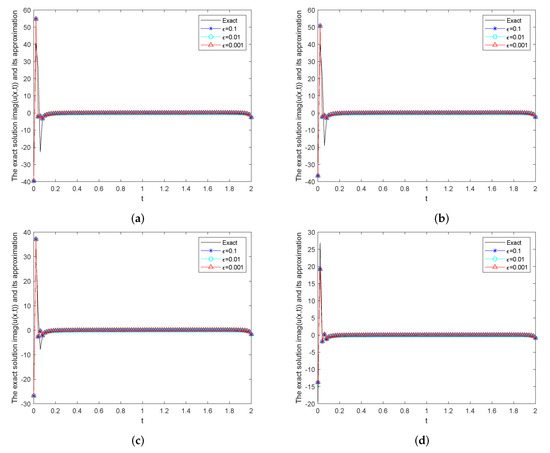
Figure 1. The imaginary part of the exact solution and its fractional Landweber regularization approximation solution for Example 1 with $\alpha =0.1$ and $\epsilon =0.1,0.01,0.001$. (a) $x=0$; (b) $x=0.1$; (c) $x=0.5$; (d) $x=0.9$.

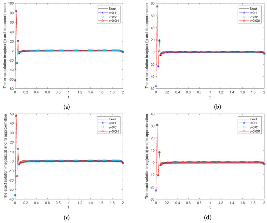
Figure 2. The imaginary part of the exact solution and its fractional Landweber regularization approximation solution for Example 1 with $\alpha =0.5$ and $\epsilon =0.1,0.01,0.001$. (a) $x=0$; (b) $x=0.1$; (c) $x=0.5$; (d) $x=0.9$.

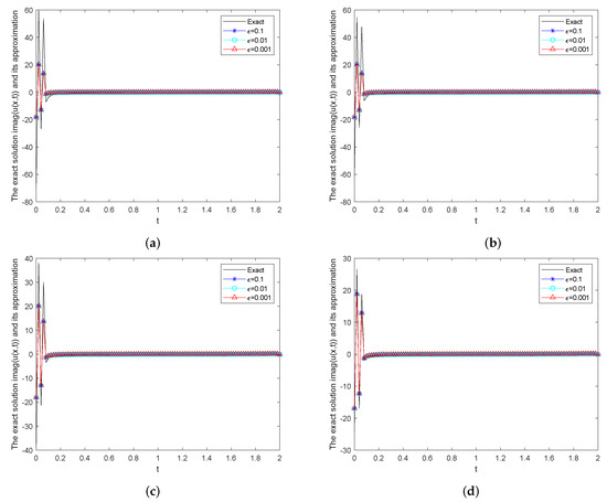
Figure 3. The imaginary part of the exact solution and its fractional Landweber regularization approximation solution for Example 1 with $\alpha =0.9$ and $\epsilon =0.1,0.01,0.001$. (a) $x=0$; (b) $x=0.1$; (c) $x=0.5$; (d) $x=0.9$.

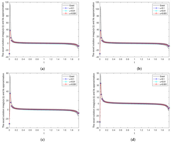
Figure 4. The imaginary part of the exact solution and its fractional Landweber regularization approximation solution for Example 2 with $\alpha =0.1$ and $\epsilon =0.1,0.01,0.001$. (a) $x=0$; (b) $x=0.1$; (c) $x=0.5$; (d) $x=0.9$.

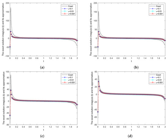
Figure 5. The imaginary part of the exact solution and its fractional Landweber regularization approximation solution for Example 2 with $\alpha =0.5$ and $\epsilon =0.1,0.01,0.001$. (a) $x=0$; (b) $x=0.1$; (c) $x=0.5$; (d) $x=0.9$.

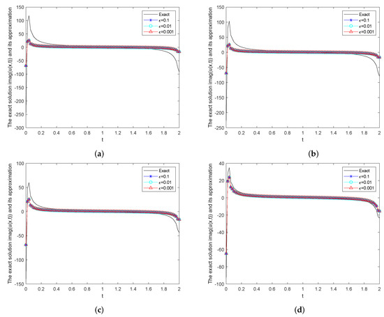
Figure 6. The imaginary part of the exact solution and its fractional Landweber regularization approximation solution for Example 2 with $\alpha =0.9$ and $\epsilon =0.1,0.01,0.001$. (a) $x=0$; (b) $x=0.1$; (c) $x=0.5$; (d) $x=0.9$.

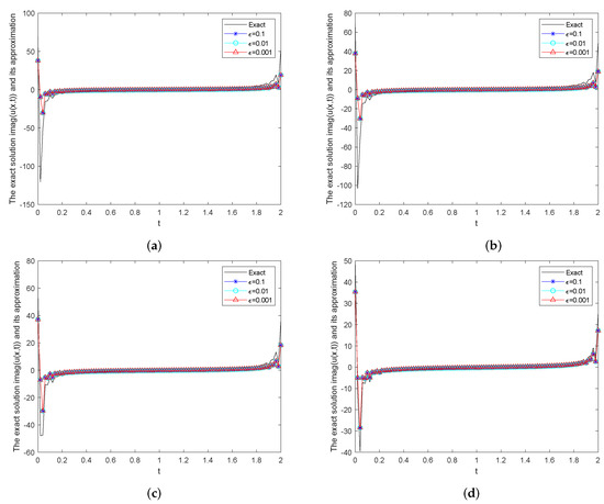
Figure 7. The imaginary part of the exact solution and its fractional Landweber regularization approximation solution for Example 3 with $\alpha =0.1$ and $\epsilon =0.1,0.01,0.001$. (a) $x=0$; (b) $x=0.1$; (c) $x=0.5$; (d) $x=0.9$.

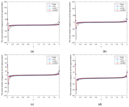
Figure 8. The imaginary part of the exact solution and its fractional Landweber regularization approximation solution for Example 3 with $\alpha =0.5$ and $\epsilon =0.1,0.01,0.001$. (a) $x=0$; (b) $x=0.1$; (c) $x=0.5$; (d) $x=0.9$.

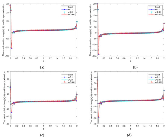
Figure 9. The imaginary part of the exact solution and its fractional Landweber regularization approximation solution for Example 3 with $\alpha =0.9$ and $\epsilon =0.1,0.01,0.001$. (a) $x=0$; (b) $x=0.1$; (c) $x=0.5$; (d) $x=0.9$.

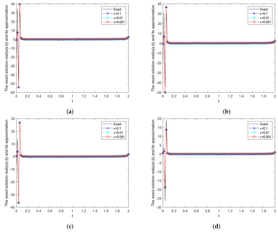
Figure 10. The real part of the exact solution and its fractional Landweber regularization approximation solution for Example 1 with $\alpha =0.1$ and $\epsilon =0.1,0.01,0.001$. (a) $x=0$; (b) $x=0.1$; (c) $x=0.5$; (d) $x=0.9$.

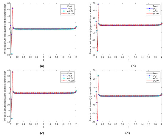
Figure 11. The real part of the exact solution and its fractional Landweber regularization approximation solution for Example 1 with $\alpha =0.5$ and $\epsilon =0.1,0.01,0.001$. (a) $x=0$; (b) $x=0.1$; (c) $x=0.5$; (d) $x=0.9$.

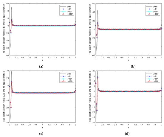
Figure 12. The real part of the exact solution and its fractional Landweber regularization approximation solution for Example 1 with $\alpha =0.9$ and $\epsilon =0.1,0.01,0.001$. (a) $x=0$; (b) $x=0.1$; (c) $x=0.5$; (d) $x=0.9$.

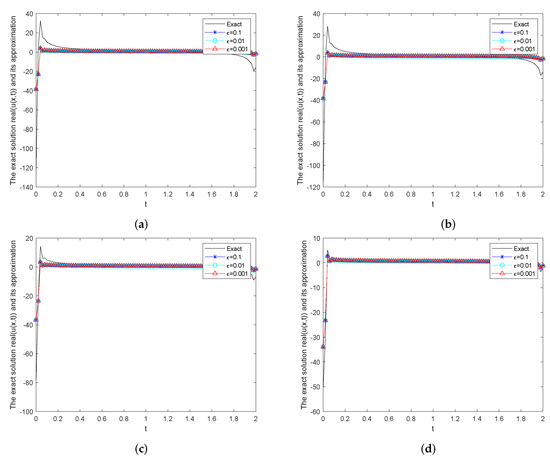
Figure 13. The real part of the exact solution and its fractional Landweber regularization approximation solution for Example 2 with $\alpha =0.1$ and $\epsilon =0.1,0.01,0.001$. (a) $x=0$; (b) $x=0.1$; (c) $x=0.5$; (d) $x=0.9$.

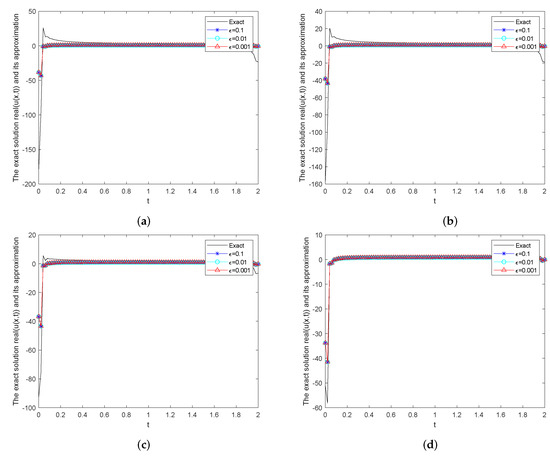
Figure 14. The real part of the exact solution and its fractional Landweber regularization approximation solution for Example 2 with $\alpha =0.5$ and $\epsilon =0.1,0.01,0.001$. (a) $x=0$; (b) $x=0.1$; (c) $x=0.5$; (d) $x=0.9$.

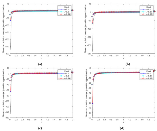
Figure 15. The real part of the exact solution and its fractional Landweber regularization approximation solution for Example 2 with $\alpha =0.9$ and $\epsilon =0.1,0.01,0.001$. (a) $x=0$; (b) $x=0.1$; (c) $x=0.5$; (d) $x=0.9$.

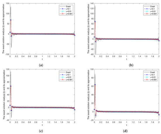
Figure 16. The real part of the exact solution and its fractional Landweber regularization approximation solution for Example 3 with $\alpha =0.1$ and $\epsilon =0.1,0.01,0.001$. (a) $x=0$; (b) $x=0.1$; (c) $x=0.5$; (d) $x=0.9$.

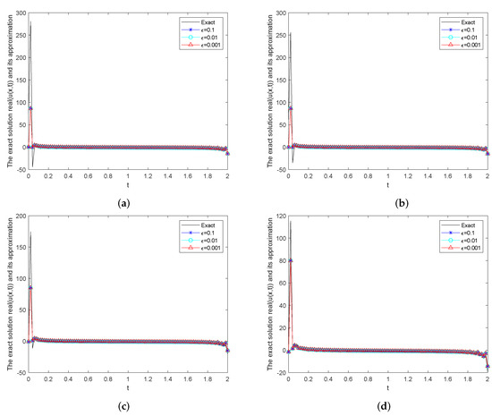
Figure 17. The real part of the exact solution and its fractional Landweber regularization approximation solution for Example 3 with $\alpha =0.5$ and $\epsilon =0.1,0.01,0.001$. (a) $x=0$; (b) $x=0.1$; (c) $x=0.5$; (d) $x=0.9$.

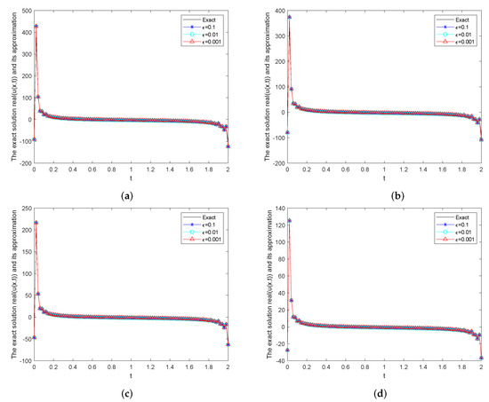
Figure 18. The real part of the exact solution and its fractional Landweber regularization approximation solution for Example 3 with $\alpha =0.9$ and $\epsilon =0.1,0.01,0.001$. (a) $x=0$; (b) $x=0.1$; (c) $x=0.5$; (d) $x=0.9$.

From the above three examples, it can be proved that the fitting effect of the function with good properties is far better than that of the function with poor properties for different functions. For the ill-posed problems mentioned in this paper, the fractional Landweber iterative regularization method is effective.

Table 2, Table 3 and Table 4 show the CPU time required to deal with the inverse problem by using the fractional Landweber iterative regularization method in numerical implementation. From Table 1, Table 2 and Table 3, it can be found that the CPU time required for the fractional Landweber iterative regularization method is longer and longer along with increasing $\alpha$.

Table 2. Example 1: CPU-time fractional Landweber iterative regularization method with $\epsilon =0.1,0.01,0.001$.

x		0	0.1	0.5	0.9
$\alpha =0.1$	imaginary part	3.8528	3.5900	3.5390	3.0305
	real part	3.6872	3.5840	3.3953	2.8516
$\alpha =0.5$	imaginary part	3.8038	3.2990	3.4192	3.3340
	real part	3.2198	3.2599	3.7458	3.6131
$\alpha =0.9$	imaginary part	2.7837	3.0263	2.6288	2.5222
	real part	2.5062	2.6698	2.4578	2.4390

Table 3. Example 2: CPU-time fractional Landweber iterative regularization method with $\epsilon =0.1,0.01,0.001$.

x		0	0.1	0.5	0.9
$\alpha =0.1$	imaginary part	2.9048	2.4628	3.1220	2.6568
	real part	2.4462	2.5175	2.4988	2.4919
$\alpha =0.5$	imaginary part	2.7741	3.1374	2.5543	2.5815
	real part	2.5790	2.3636	2.6282	2.4231
$\alpha =0.9$	imaginary part	3.4433	2.6319	2.9360	2.3540
	real part	2.4825	2.6784	2.3447	2.4814

Table 4. Example 3: CPU-time fractional Landweber iterative regularization method with $\epsilon =0.1,0.01,0.001$.

x		0	0.1	0.5	0.9
$\alpha =0.1$	imaginary part	8.8441	3.3292	2.5647	2.9310
	real part	3.3262	2.4933	2.6226	2.5787
$\alpha =0.5$	imaginary part	2.5854	3.1151	2.7623	2.7536
	real part	2.8532	2.6008	2.4003	2.4627
$\alpha =0.9$	imaginary part	3.8097	4.1494	3.5712	3.6969
	real part	3.9111	3.3240	3.2959	3.2857

6. Conclusions

In this paper, the inverse identification of wave function for a potential-free field inverse thermal fractional Schrödinger equation with boundary condition is studied. The fractional Landweber iterative regularization method is used to solve the ill-posed problem. Moreover, the convergence error estimates between the exact solution and the regularized solution are given based on a priori regularization parameter selection rules and a posteriori regularization parameter selection rules, respectively. In addition, three numerical examples are given to demonstrate the effectiveness and practicability of the fractional Landweber iterative regularization method. When $s=1$ in (16), the fractional Landweber iterative regularization method is the Landweber iterative regularization method, and the two methods can be compared. The fractional Landweber iterative regularization method requires fewer iteration steps than the Landweber iterative regularization method, that is, this method requires less iteration time. Compared with the standard quasi-boundary regularization method I have been exposed to so far, the fractional Landweber iterative regularization method does not appear saturated, while the quasi-boundary regularization method appears saturated. In conclusion, the fractional Landweber regularization method is superior to the Landweber iterative regularization method and the standard quasi-boundary regularization method.

References

- Fine, D.S.; Stephen, S. Path integrals, supersymmetric quantum mechanics, and the atiyah-singer index theorem for twisted dirac. J. Math. Phys. 2017, 58, 012102. [Google Scholar] [CrossRef]
- Naber, M. Time fractional Schrödinger equation. J. Math. Phys. 2004, 45, 3339–3352. [Google Scholar] [CrossRef]
- Berezin, F.A.; Shubin, M.A. The Schrödinger equation. Math. Comput. Simulat. 1992, 34, 88–89. [Google Scholar]
- Baudouin, L.; Puel, J.P. Uniqueness and stability in an inverse problem for the Schrödinger equation. Inverse Prob. 2007, 18, 1537. [Google Scholar] [CrossRef]
- Schneider, W.R.; Wyss, W. Fractional diffusion and wave equation. J. Math. Phys. 1989, 30, 134–144. [Google Scholar] [CrossRef]
- Sun, H.G.; Chen, W.; Liang, Y.J.; Hu, S. Fractional derivative anomalous diffusion equation modeling prime number distribution. Fract. Calc. Appl. Anal. 2015, 18, 154–157. [Google Scholar]
- Ricardo, A. A caputo fractional derivative of a function with respect to another function. Commun. Nonlinear. Sci. 2017, 44, 460–481. [Google Scholar]
- Wei, Z.l.; Dong, W.; Che, J.L. Periodic boundary value problems for fractional differential equations involving a Riemann-Liouville fractional derivative. Nonlinear. Anal. 2010, 73, 3232–3238. [Google Scholar] [CrossRef]
- Zemliak, A.M. Analog system design problem formulation by optimum control theory. Ieice T. Fund. Electr. 2001, 84, 2029–2041. [Google Scholar]
- Brenier, Y. The initial value problem for the euler equations of incompressible fluids viewed as a concave maximization problem. Commun. Math. Phys. 2018, 364, 579–605. [Google Scholar] [CrossRef]
- Anikonov, Y.E.; Neshchadim, M.V. On analytical methods in the theory of inverse problems for hyperbolic equations. J. Appl. Ind. Math. 2011, 5, 506–518. [Google Scholar] [CrossRef]
- Etingof, P.I. Inverse problems of potential theory and flows in porous media with time-dependent free boundary. Comput. Math. Appl. 1991, 22, 93–99. [Google Scholar] [CrossRef]
- Wei, T.; Li, X.L.; Li, Y.S. An inverse time-dependent source problem for a time-fractional diffusion equation. Inverse Prob. 2018, 32, 085003. [Google Scholar] [CrossRef]
- Sergei, A.; Avdonin, V.S.; Ramdani, K. Reconstructing the potential for the one-dimensional Schrödinger equation from boundary measurements. Ima J. Math. Control. I. 2014, 31, 137–150. [Google Scholar]
- Shvetsov-Shilovski, N.I.; RäSäNen, E. Stable and efficient momentum-space solutions of the time-dependent Schrödinger equation for one-dimensional atoms in strong laser fields. J. Comput. Phys. 2014, 279, 174–181. [Google Scholar] [CrossRef]
- Faustov, R.N.; Galkin, V.O.; Tatarintsev, A.V.; Vshivtsev, A.S. Spectral problem of the radial Schrödinger equation with confining power potentials. Theor. Math. Phys. 1997, 113, 1530–1542. [Google Scholar] [CrossRef]
- Knops, R.J. Book Review: Ill-posed problems of mathematical physics and analysis. Bull. Am. Math. Soc. 1988, 19, 332–338. [Google Scholar] [CrossRef]
- Marin, L.; Elliott, L.; Heggs, P.J.; Ingham, D.B.; Lesnic, D.; Wen, X. BEM solution for the cauchy problem associated with helmholtz-type equations by the landweber method. Eng. Anal. Bound. Elem. 2004, 28, 1025–1034. [Google Scholar] [CrossRef]
- Scherzer, O. Convergence criteria of iterative methods based on landweber iteration for solving nonlinear problems. J. Math. Anal. Appl. 1995, 194, 911–933. [Google Scholar] [CrossRef]
- Han, Y.; Xiong, X.; Xue, X. A fractional landweber method for solving backward time-fractional diffusion problem. Comput. Math. Appl. 2019, 78, 81–91. [Google Scholar] [CrossRef]
- Jiang, S.Z.; Wu, Y.J. Recovering space-dependent source for a time-space fractional diffusion wave equation by fractional Landweber method. Inverse Probl. Sci. En. 2020, 29, 1–22. [Google Scholar] [CrossRef]
- Fu, C.L.; Xiong, X.T.; Qian, Z. Fourier regularization for a backward heat equation. J. Math. Anal. Appl. 2007, 31, 472–480. [Google Scholar] [CrossRef]
- Dou, F.F.; Fu, C.L.; Yang, F.L. Optimal error bound and Fourier regularization for identifying an unknown source in the heat equation. J. Comput. Appl. Math. 2009, 230, 728–737. [Google Scholar] [CrossRef]
- Yang, F.; Fu, J.L.; Li, X.X. A potential-free field inverse Schrödinger problem: Optimal error bound analysis and regularization method. Inverse Probl. Sci. En. 2020, 28, 1209–1252. [Google Scholar] [CrossRef]
- Yang, F.; Wu, H.H.; Li, X.X. Three regularization methods for identifying the initial value of homogeneous anomalous secondary diffusion equation. Math. Method. Appl. Sci. 2021, 44, 13723–13755. [Google Scholar] [CrossRef]
- Qian, A.; Xiong, X.; Wu, Y. On a quasi-reversibility regularization method for a cauchy problem of the helmholtz equation. J. Comput. Appl. Math. 2010, 233, 1969–1979. [Google Scholar] [CrossRef]
- Yang, F.; Fu, J.L. The method of simplified Tikhonov regularization for dealing with the inverse time-dependent heat source problem. Comput. Math. Appl. 2010, 60, 1228–1236. [Google Scholar] [CrossRef]
- Djennadi, S.; Shawagfeh, N.; Arqub, O.A. A fractional Tikhonov regularization method for an inverse backward and source problems in the time-space fractional diffusion equations. Chaos Soliton. Fract. 2021, 150, 111127. [Google Scholar] [CrossRef]
- Ivanchov, M.I. The inverse problem of determining the heat source power for a parabolic equation under arbitrary boundary conditions. J. Math. Sci. 1998, 88, 432–436. [Google Scholar] [CrossRef]
- Thorsten, H. Regularization of exponentially ill-posed problems. Numer. Func. Anal. Opt. 2000, 21, 439–464. [Google Scholar]
- Vaiter, S.; Peyré, G.; Fadili, J.M. Partly smooth regularization of inverse problems. Inverse Probl. Imag. 2014, 5303, 57–68. [Google Scholar]
- Tautenhahn, U. Optimal stable solution of cauchy problems for elliptic equations. Z. Anal. Anwend. 1996, 15, 961–984. [Google Scholar] [CrossRef]
- Tautenhahn, U. Optimality for ill-posed problems under general source conditions. Numer. Func. Anal. Opt. 2007, 19, 377–398. [Google Scholar] [CrossRef]
Publisher’s Note: MDPI stays neutral with regard to jurisdictional claims in published maps and institutional affiliations. |
© 2022 by the authors. Licensee MDPI, Basel, Switzerland. This article is an open access article distributed under the terms and conditions of the Creative Commons Attribution (CC BY) license (https://creativecommons.org/licenses/by/4.0/).