Modeling Extreme Values Utilizing an Asymmetric Probability Function

Abstract

In this article, a new flexible probability density function with three parameters is proposed for modeling asymmetric data (positive and negative) with different types of kurtosis (mesokurtic, leptokurtic and platykurtic). Some of its statistical and reliability properties, including hazard rate function, moments, moment generating function, incomplete moments, mean deviations, moment of the residual life, moment of the reversed residual life, and order statistics are derived. Its hazard rate function can be either constant, increasing-constant, decreasing-constant, U shape, upside down shape or upside down-U shape. Seven classical estimation methods are considered to estimate the unknown model parameters. Monte Carlo simulation experiments are performed to compare the performance of the seven different estimation methods. Finally, a distinctive asymmetric real data application is analyzed for illustrating the flexibility of the new model.

1. Introduction

Recently, Nadarajah and Haghighi [1] presented and studied a new lifetime model and pointed out that its probability density function (PDF) has a zero mode. A random variable (RV) $Z$ is said to have Nadarajah and Haghighi (NH) model if its survival function (SF) and PDF are given by

$$R_c\left(z\right)=e^{1-{(1+z)}^c}; z\ge 0,c>0,$$

(1)

and

$$g_c\left(z\right)=c{(1+z)}^{c-1}{e}^{1-{(1+z)}^c}; z\ge 0,c>0,$$

(2)

respectively, where $c$ is a shape parameter. Nadarajah and Haghighi [1] considered (2) as an alternative to the exponential (Exp), gamma (Gam), Weibull (W) and exponentiated-exponential (ExpExp) distributions. Several extensions of the NH model can be cited, such as the exponentiated NH (E-NH) model by Lemonte [2], the Gam NH (Gam-NH) and Poisson Gam NH (PGam-NH) by Ortega et al. [3], transmuted NH (Tr-NH) by Ahmed et al. [4], Kumaraswamy NH (Kuw-NH) by Lim [5], modified NH (Mo-NH) by El-Damcese and Ramadan [6], Marshall–Olkin NH (MO-NH) by Lemonte et al. [7], Topp–Leone NH (TL-NH) by Yousof and Korkmaz [8], beta NH (B-NH) by Dias [9], inverted NH (I-NH) by Tahir et al. [10], and NH Lindley (NH-L) by Pena et al. [11]. The PDF and cumulative distribution function (CDF) of the Topp–Leone exponentiated-G(TLE-G) family are given by

$$f_{a,b,\underset{\_}{\mathit{\Omega }}}\left(z\right)=2ab{g}_{\underset{\_}{\mathit{\Omega }}}\left(z\right)G_{\underset{\_}{\mathit{\Omega }}}{\left(z\right)}^{ba-1}\left[1-G_{\underset{\_}{\mathit{\Omega }}}{\left(z\right)}^b\right]{\left[2-G_{\underset{\_}{\mathit{\Omega }}}{\left(z\right)}^b\right]}^{a-1}$$

(3)

and

$$F_{a,b,\underset{\_}{\mathit{\Omega }}}\left(z\right)={\left\{G_{\underset{\_}{\mathit{\Omega }}}{\left(z\right)}^b\left[2-G_{\underset{\_}{\mathit{\Omega }}}{\left(z\right)}^b\right]\right\}}^a,$$

(4)

respectively, where $G_{\underset{\_}{\mathit{\Omega }}}\left(z\right)=1-R_c\left(z\right)$ is the CDF of any baseline model and $g_{\underset{\_}{\mathit{\Omega }}}\left(z\right)=d{G}_{\underset{\_}{\mathit{\Omega }}}\left(z\right)/dx$ is the PDF of any baseline model. For $b=1,$ we get the TL family. By inserting (1) and (2) into (3), we can write the PDF of the TLE-NH model as

$$f\left(z\right)=2abc{(1+z)}^{c-1}{e}^{1-{(1+z)}^c}{H}_{ab-1,c}\left(z\right)\left[1-H_{b,c}\left(z\right)\right]{\left[2-H_{b,c}\left(z\right)\right]}^{a-1},$$

(5)

where $H_{{\gamma }_1,{\gamma }_2}\left(z\right)={\left[1-e^{1-{(1+z)}^{{\gamma }_2}}\right]}^{{\gamma }_1}.$ After a quick study of TLE-NH properties, different classical estimation methods under uncensored schemes are considered, such as the maximum likelihood (ML), Anderson–Darling (AD), ordinary least squares (OLS), Cramér–von Mises (CVM), weighted least squares (WLS), left-tail Anderson–Darling (LTAD), and right-tail Anderson–Darling (RTAD) methods. Numerical simulations are performed for comparing the estimation approaches using different sample sizes for three different combinations of parameters. The corresponding CDF is given by

$$F\left(z\right)={\left\{H_{b,c}\left(z\right)\left[2-H_{b,c}\left(z\right)\right]\right\}}^a.$$

(6)

For $b=1,$ the TLE-NH reduces to the TL-NH (see [8]). We provide some plots of the PDF and hazard rate function (HRF) of the TLE-NH model to show its flexibility. The CDF in (6) can be expressed as

$$F\left(z\right)={\displaystyle \sum }_{{\varsigma }_1=0}^{\infty }{C}_{\left({\varsigma }_1\right)}{H}_{{\varsigma }_1^{•},c}\left(z\right){|}_{{\varsigma }_1^{•}=\left(a+{\varsigma }_1\right)b},$$

(7)

where $C_{\left({\varsigma }_1\right)}={\left(-1\right)}^{{\varsigma }_1}{\left(\frac{1}{2}\right)}^{{\varsigma }_1-a}\left(\begin{array}{c}a\\ {\varsigma }_1\end{array}\right)$ and $H_{{\varsigma }_1^{•},c}\left(z\right)=G^{{\varsigma }_1^{•}}\left(z;c\right)$ is the CDF of the E-NH model with power parameter ${\varsigma }_1^{•}$. The corresponding TLE-NH density function can be formulated as

$$f\left(z\right)={\displaystyle \sum }_{{\varsigma }_1=0}^{\infty }{C}_{\left({\varsigma }_1\right)} h_{{\varsigma }_1^{•},c}\left(z\right),$$

(8)

where $h_{{\varsigma }_1^{•},c}\left(z\right)$ is the E-NH PDF with power parameter ${\varsigma }_1^{•}$. Figure 1a displays some plots of the TLE-NH density for some parameter values of $a$, $b$ and $c$. The plots of the HRF of the TLE-NH model for some parameter values of $a$, $b$ and $c$ are obtained in Figure 1b.

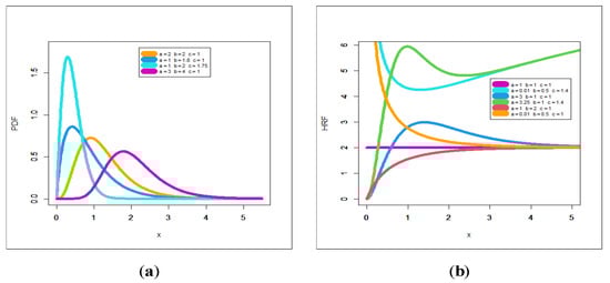
Figure 1. Plots of the TLE-NH PDF (a) and HRF (b) for some parameter values.

Figure 1a shows that the PDF of the new version has right skew tails with different shapes whereas Figure 1b shows that the HRF of the TLE-NH has many important failure rates such as “constant ($a=1$, $b=1$ and $c=1$)”, “increasing-constant ($a=1$, $b=2$ and $c=1$)”, “decreasing-constant ($a=0.01$, $b=0.5$ and $c=1$)”, “U shape ($a=1$, $b=0.5$ and $c=1.4$)”, “upside down shape ($a=3$, $b=1$ and $c=1$)” and “upside down-U shape ($a=3.25$, $b=1$ and $c=1.4$)”.

We are motivated to introduce and study the TLE-NH model for the following reasons:

i. 

The new density in (5) can be “asymmetric unimodal and right skewed” with many useful shapes.

ii. 

The HRF of the new model can be constant, increasing-constant, bathtub (U-HRF), decreasing-constant and upside-down (reversed U-HRF). These characteristics give a great advantage to the TLE-NH model for analyzing the data sets in which its HRF can be constant, increasing-constant bathtub, decreasing-constant or upside down- bathtub.

iii. 

The new TLE-NH model is recommended for modeling the remission times (in months) of the bladder cancer patients. The bladder cancer data have some extreme values.

iv. 

Also, its nonparametric Kernel density estimation is asymmetric with heavy tail to the right. Therefore, the TLE-NH model could be useful asymmetric real data especially the unimodal symmetric heavy tailed right skewed data and the bimodal symmetric heavy tailed right skewed data.

v. 

On the other hand, the new TLE-NH model is flexible enough to exhibit the asymmetric densities and right heavy tail shapes as illustrated in Figure 1a.

vi. 

Moreover, the HRF of the bladder cancer patients is upside-down; this property matches with our new model which contains the upside-down HRF as illustrated in Figure 1b. It is vital to mention that the presented class of probabilistic distributions suitable for modeling asymmetric data also have an important utilization in insurance (see Maciak et al. [12] for more details) and in dependence modeling (see Gijbels et al. [13]).

vii. 

The range of the skewness of the TLE-NH model is falling in the interval ($-0.92852, 43.03816$). However, the skewness of the standard baseline NH model is falling in the interval ($0.27557, 2$). The wide range of the skewness gives priority to the TLE-NH model in modeling and future prediction since many real-life datasets are negatively skewed. The standard baseline NH model cannot be useful in such cases (see Tables 1 and 2 and Figures 2 and 3).

viii. 

The kurtosis of the TLE-NH model is located between $3.03238$ and $2722.165$, however the kurtosis of the NH model starts from $3.23056$ to $9$. Thus, the TLE-NH extension could be useful for mesokurtic, leptokurtic and platykurtic data sets (see Tables 1 and 2 and Figures 2 and 3).

ix. 

The estimation persuaders of the TLE-NH model can be performed under the maximum likelihood, Anderson–Darling, ordinary least squares, Cramér–von Mises, weighted least squares, left-tail Anderson–Darling, and right-tail Anderson–Darling methods. Although all estimation methods perform well, the weighted least squares estimation method is the best in real data modeling, with slight differences in results.

2. Properties

2.1. Moments

The $q^{th}$ ordinary moment of $Z$ is given by ${\mu }_{q,Z}^{\prime }=E\left(Z^q\right)={\displaystyle \sum }_{{\varsigma }_1=0}^{\infty }{C}_{\left({\varsigma }_1\right)}\underset{0}{\overset{\infty }{{\displaystyle \int }}}{z}^q{h}_{{\varsigma }_1^{•},c}\left(z\right)dz.$ Then we obtain

$${\mu }_{q,Z}^{\prime }={\displaystyle \sum }_{{\varsigma }_1,{\hslash }_1=0}^{\infty }{\displaystyle \sum }_{{\hslash }_2=0}^q{V}_{\left({\varsigma }_1,{\hslash }_1,{\hslash }_2\right)}^{\left({\varsigma }_1^{•},q\right)}\Gamma \left(1+\frac{{\hslash }_2}{c},{\hslash }_1+1\right),$$

(9)

where $V_{\left({\varsigma }_1,{\hslash }_1,{\hslash }_2\right)}^{\left({\varsigma }_1^{•},q\right)}=C_{\left({\varsigma }_1\right)}{V}_{{\hslash }_1,{\hslash }_2}^{\left({\varsigma }_1^{•},q\right)}$, $V_{{\hslash }_1,{\hslash }_2}^{\left({\varsigma }_1^{•},q\right)}={\varsigma }_1^{•}{\left(-1\right)}^{q+{\hslash }_1-{\hslash }_2}{e}^{{\hslash }_1+1}{\left({\hslash }_1+1\right)}^{-\left(1+\frac{{\hslash }_2}{c}\right)}\left(\begin{array}{c}{\varsigma }_1^{•}-1\\ {\hslash }_1\end{array}\right)\left(\begin{array}{c}q\\ {\hslash }_2\end{array}\right)$ and $\Gamma \left(c,z\right)=\underset{z}{\overset{\infty }{{\displaystyle \int }}}{z}^{c-1}{e}^{-z}dz$ refers to the complementary incomplete Gamma function. The moments in (9) reduce to ($\forall$ ${\varsigma }_1^{•}>0$ integer)

$${\mu }_{q,Z}^{\prime }={\displaystyle \sum }_{{\varsigma }_1=0}^{\infty }{\displaystyle \sum }_{{\hslash }_1=0}^{{\varsigma }_1^{•}-1}{\displaystyle \sum }_{{\hslash }_2=0}^q{V}_{\left({\varsigma }_1,{\hslash }_1,{\hslash }_2\right)}^{\left({\varsigma }_1^{•},q\right)}\Gamma \left(1+\frac{{\hslash }_2}{c},{\hslash }_1+1\right),$$

(10)

when $q=1$ in (9) and (10), we have the mean of $Z$. The $q^{th}$ central moment of $Z$, say ${\mu }_{q,Z}$, is

$${\mu }_{q,Z}=E{(z-\mu )}^q={\displaystyle \sum }_{h=0}^q{(-1)}^h\left(\begin{array}{c}q\\ h\end{array}\right){({\mu }_1^{\prime })}^q {\mu }_{q-h}^{\prime }.$$

Table 1 lists the expected value $\left(E\left(Z\right)\right),$ variance $\left(V\left(Z\right)\right),$ skewness $\left(S\left(Z\right)\right)$ and kurtosis $\left(K\left(Z\right)\right)$ for the TLE-NH model, whereas Table 2 reports the $E\left(Z\right),$ $V\left(Z\right),$ $S\left(Z\right)$ and $K\left(Z\right)$ values for the NH model. From Table 1 and Table 2, we note that the range of $S\left(Z\right)$ of the TLE-NH model is ($-0.92852,43.03816$), however the $S\left(Z\right)$ of the NH model is ($0.27557,2$). The $K\left(Z\right)$ of the TLE-NH model is located between $3.03238$ and $2722.165$, however the $K\left(Z\right)$ of the NH model starts from $3.23056$ to $9$. Figure 2 shows three-dimensional (3-D) skewness plots for $c=$0.01, 0.25, 5.75, 75, 150, 1000. Figure 3 shows 3-D kurtosis plots for $c=$0.01, 0.25, 5.75, 75, 150, 1000. Figure 2 and Figure 3 illustrate how $S\left(Z\right)$ and $K\left(Z\right)$ changes with respect to the new parameter $c$. Table 1 and plots of Figure 2 Figure 3 show that the proposed model can be utilized for analyzing the asymmetric data with different types of kurtosis.

Table 1. E(Z), V(Z), S(Z) and K(Z) for the TLE-NH model.

a	b	c	E(Z)	V(Z)	S(Z)	K(Z)
0.001	1.0	1.0	0.001286	0.0008056	43.03816	2722.165
0.01			0.012572	0.0078321	13.73513	279.9879
0.1			0.104002	0.0621733	4.697541	35.42657
0.25			0.208241	0.1193405	3.268103	18.69152
0.5			0.326534	0.1790888	2.557750	12.62371
1.0			0.5	0.25	2.0	9.0
1.5			0.665002	0.2803381	1.784458	7.855008
0.001	3.5	5.0	0.001209	0.0001259	14.00467	245.1215
0.1			0.080019	0.0037463	1.444700	4.787573
1.0			0.177359	0.0045912	0.402047	3.032383
3.0			0.222693	0.0061278	−0.92852	4.867656
0.1	0.1	1.25	0.001482	0.0005384	32.69074	1578.728
	0.5		0.026813	0.0108739	7.517766	84.14104
	1.0		0.079014	0.0331868	4.274762	28.70463
	5.0		0.558848	0.1322969	2.206003	7.477113
	6.0		0.663141	0.1200882	3.039792	7.785333
0.25	1.5	0.5	1.019356	2.8743150	4.829448	47.14539
		1.0	0.353175	0.1882723	2.492174	12.09759
		5.0	0.055709	0.0032452	1.602556	5.778513
		10.0	0.027117	0.0007387	1.521412	5.350372
		20.0	0.013381	0.0001763	1.412999	5.279472

Table 2. E(Z), V(Z), S(Z) and K(Z) for the NH model.

c	E(Z)	V(Z)	S(Z)
1.00	1.0	1.0	2.0
1.50	0.5516834	0.2353814	1.473465
2.00	0.3789361	0.0985353	1.253915
2.50	0.2881511	0.0531792	1.133407
3.00	0.2323270	0.0330535	1.057228
4.00	0.1673480	0.0162348	0.966298
5.00	0.1307332	0.0095934	0.913879
10.0	0.0623942	0.0020517	0.813496
15.0	0.0409678	0.0008665	0.781278
20.0	0.0304945	0.0004752	0.764709
25.0	0.0242857	0.0002996	0.825042
30.0	0.0201773	0.0002059	0.275571

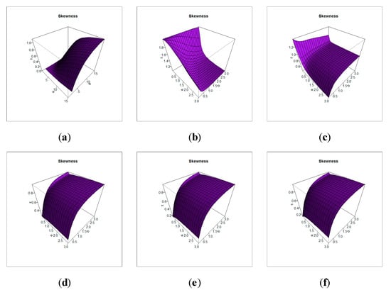
Figure 2. 3-D skewness plots for $c=$ 0.01, 0.25, 5.75, 75, 150, 1000 (a–f).

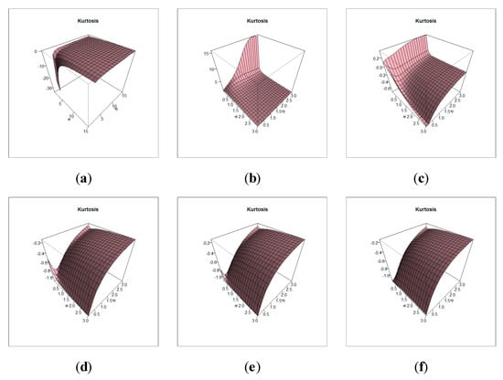
Figure 3. 3-D kurtosis plots for $c=$ 0.01, 0.25, 5.75, 75, 150, 1000 (a–f).

2.2. Moment Generating Function (MGF)

The MGF $M_Z\left(\tau \right)=E\left(e^{\tau Z}\right)$ of $Z$ can be derived from Equation (9) or (10) as

$$M_Z\left(\tau \right)={\displaystyle \sum }_{{\varsigma }_1,{\hslash }_1,q=0}^{\infty }{\displaystyle \sum }_{{\hslash }_2=0}^q\frac{{\tau }^q}{q!}{V}_{\left({\varsigma }_1,{\hslash }_1,{\hslash }_2\right)}^{\left({\varsigma }_1^{•},q\right)}\Gamma \left(1+\frac{{\hslash }_2}{c},{\hslash }_1+1\right),$$

or $\forall$ ${\varsigma }_1^{•}>0$ integer we have

$$M_Z\left(\tau \right)={\displaystyle \sum }_{{\varsigma }_1,q=0}^{\infty }{\displaystyle \sum }_{{\hslash }_1=0}^{{\varsigma }_1^{•}-1}{\displaystyle \sum }_{{\hslash }_2=0}^q\frac{{\tau }^q}{q!}{V}_{\left({\varsigma }_1,{\hslash }_1,{\hslash }_2\right)}^{\left({\varsigma }_1^{•},q\right)}\Gamma \left(1+\frac{{\hslash }_2}{c},{\hslash }_1+1\right).$$

2.3. Incomplete Moments (I-Ms)

The $s^{th}$ I-M, say $I_{s,Z}\left(\tau \right)$, of $Z$ can be expressed from (8) as $I_{s,Z}\left(\tau \right)={\displaystyle \sum }_{{\varsigma }_1=0}^{\infty }{C}_{\left({\varsigma }_1\right)}\underset{-\infty }{\overset{\tau }{{\displaystyle \int }}}{z}^s{h}_{{\varsigma }_1^{•},c}\left(z\right)dz,$ then

$$I_{s,Z}\left(\tau \right)={\displaystyle \sum }_{{\varsigma }_1,{\hslash }_1=0}^{\infty }{\displaystyle \sum }_{{\hslash }_2=0}^s{V}_{\left({\varsigma }_1,{\hslash }_1,{\hslash }_2\right)}^{\left({\varsigma }_1^{•},s\right)}\left[\Gamma \left(1+\frac{{\hslash }_2}{c},\left({\hslash }_1+1\right)\right)-\Gamma \left(1+\frac{{\hslash }_2}{c},\left({\hslash }_1+1\right){(\tau +1)}^c\right)\right],$$

or $\forall$ ${\varsigma }_1^{•}>0$ integer we have

$$I_{s,Z}\left(\tau \right)={\displaystyle \sum }_{{\varsigma }_1=0}^{\infty }{\displaystyle \sum }_{{\hslash }_1=0}^{{\varsigma }_1^{•}-1}{\displaystyle \sum }_{{\hslash }_2=0}^s{V}_{\left({\varsigma }_1,{\hslash }_1,{\hslash }_2\right)}^{\left({\varsigma }_1^{•},s\right)}\left[\Gamma \left(1+\frac{{\hslash }_2}{c},\left({\hslash }_1+1\right)\right)-\Gamma \left(1+\frac{{\hslash }_2}{c},\left({\hslash }_1+1\right){(\tau +1)}^c\right)\right].$$

2.4. The $m^{th}$ Moment of the Residual Life (MoRL)

The $m^{th}$ MoRL can be formulated as

$$l_{m,Z}\left(\tau \right){|}_{\left(z>\tau \mathrm{and}m=1,2,\dots \right)}=E[\left(Z-\tau {)}^m\right]=\frac{1}{1-F\left(\tau \right)}\underset{\tau }{\overset{\infty }{{\displaystyle \int }}}{(z-\tau )}^{m}dF\left(z\right).$$

Then, the $m^{th}$ MoRL of the TLE-NH model can be reported by

$$l_{m,Z}\left(\tau \right)=\frac{1}{1-F\left(\tau \right)}{\displaystyle \sum }_{{\varsigma }_1,{\hslash }_1=0}^{\infty }{\displaystyle \sum }_{{\hslash }_2=0}^m{V}_{\left({\varsigma }_1,{\hslash }_1,{\hslash }_2\right)}^{\left[1\right]}\Gamma \left(1+\frac{{\hslash }_2}{c},\left({\hslash }_1+1\right)\right),$$

where $V_{\left({\varsigma }_1,{\hslash }_1,{\hslash }_2\right)}^{\left[1\right]}=C_{\left({\varsigma }_1\right)}^{\left[1\right]}{V}_{{\hslash }_1,{\hslash }_2}^{\left({\varsigma }_1^{•},m\right)}$ and $C_{\left({\varsigma }_1\right)}^{\left[1\right]}=C_{\left({\varsigma }_1\right)}{\displaystyle \sum }_{q=0}^m\left(\begin{array}{c}m\\ q\end{array}\right){\left(-\tau \right)}^{m-q}$ or $\forall$ ${\varsigma }_1^{•}>0$ integer we have

$$l_{m,Z}\left(\tau \right)=\frac{1}{1-F\left(\tau \right)}{\displaystyle \sum }_{{\varsigma }_1=0}^{\infty }{\displaystyle \sum }_{{\hslash }_1=0}^{{\varsigma }_1^{•}-1}{\displaystyle \sum }_{{\hslash }_2=0}^m{V}_{\left({\varsigma }_1,{\hslash }_1,{\hslash }_2\right)}^{\left[1\right]}\Gamma \left(1+\frac{{\hslash }_2}{c},\left({\hslash }_1+1\right)\right).$$

The life expectation at age $\tau$ can be defined by

$$l_{1,Z}\left(\tau \right)=\frac{1}{1-F\left(\tau \right)}{\displaystyle \sum }_{{\varsigma }_1=0}^{\infty }{\displaystyle \sum }_{{\hslash }_1=0}^{{\varsigma }_1^{•}-1}{\displaystyle \sum }_{{\hslash }_2=0}^1{V}_{\left({\varsigma }_1,{\hslash }_1,{\hslash }_2\right)}^{\left[1\right]}\Gamma \left(1+\frac{{\hslash }_2}{c},\left({\hslash }_1+1\right)\right),$$

which represents the additional expected life length for a certain unit which is alive at age $\tau$.

2.5. The $m^{th}$ Moment of the Reversed Residual Life ($M_m\left(\tau \right)$)

The $m^{th}$ moment of the reversed residual life can be expressed as

$$M_{m,Z}\left(\tau \right){|}_{\left(z\le \tau ,\tau >0\mathrm{and}m=1,2,\dots \right)}=E\left[{(\tau -Z)}^m\right]=\frac{1}{F\left(\tau \right)}\underset{0}{\overset{\tau }{{\displaystyle \int }}}{(\tau -z)}^{m}dF\left(z\right).$$

Then, the $m^{th}$ MoRRL of the TLE-NH model can be formulated as

$$M_{m,Z}\left(\tau \right)=\frac{1}{F\left(\tau \right)}{\displaystyle \sum }_{{\varsigma }_1,{\hslash }_1=0}^{\infty }{\displaystyle \sum }_{{\hslash }_2=0}^m{V}_{\left({\varsigma }_1,{\hslash }_1,{\hslash }_2\right)}^{\left[2\right]}\left[\begin{array}{c}\Gamma \left(1+\frac{{\hslash }_2}{c},\left({\hslash }_1+1\right)\right)\\ -\Gamma \left(1+\frac{{\hslash }_2}{c},\left({\hslash }_1+1\right){(1+\tau )}^c\right)\end{array}\right],$$

where $V_{\left({\varsigma }_1,{\hslash }_1,{\hslash }_2\right)}^{\left[2\right]}=C_{\left({\varsigma }_1\right)}^{\left[2\right]}{V}_{{\hslash }_1,{\hslash }_2}^{\left({\varsigma }_1^{•},q\right)}$ and $C_{{\varsigma }_1}^{\left[2\right]}=C_{\left({\varsigma }_1\right)}{\displaystyle \sum }_{q=0}^m{\left(-1\right)}^q\left(\begin{array}{c}m\\ q\end{array}\right){\tau }^{m-q}$ or $\forall$ ${\varsigma }_1^{•}>0$ integer we have

$$M_{m,Z}\left(\tau \right)=\frac{1}{F\left(\tau \right)}{\displaystyle \sum }_{{\varsigma }_1=0}^{\infty }{\displaystyle \sum }_{{\hslash }_1=0}^{{\varsigma }_1^{•}-1}{\displaystyle \sum }_{{\hslash }_2=0}^m{V}_{\left({\varsigma }_1,{\hslash }_1,{\hslash }_2\right)}^{\left[2\right]}\left[\begin{array}{c}\Gamma \left(1+\frac{{\hslash }_2}{c},\left({\hslash }_1+1\right)\right)\\ -\Gamma \left(1+\frac{{\hslash }_2}{c},\left({\hslash }_1+1\right){(\tau +1)}^c\right)\end{array}\right].$$

The mean inactivity time (MIT) is given by

$$M_{1,Z}\left(\tau \right)=\frac{1}{F\left(\tau \right)}{\displaystyle \sum }_{{\varsigma }_1,{\hslash }_1=0}^{\infty }{\displaystyle \sum }_{{\hslash }_2=0}^1{V}_{\left({\varsigma }_1,{\hslash }_1,{\hslash }_2\right)}^{\left[2\right]}\left[\begin{array}{c}\Gamma \left(1+\frac{{\hslash }_2}{c},\left({\hslash }_1+1\right)\right)\\ -\Gamma \left(1+\frac{{\hslash }_2}{c},\left({\hslash }_1+1\right){(1+\tau )}^c\right)\end{array}\right],$$

or $\forall$ ${\varsigma }_1^{•}>0$ integer we get

$$M_{1,Z}\left(\tau \right)=\frac{1}{F\left(\tau \right)}{\displaystyle \sum }_{{\varsigma }_1=0}^{\infty }{\displaystyle \sum }_{{\hslash }_1=0}^{{\varsigma }_1^{•}-1}{\displaystyle \sum }_{{\hslash }_2=0}^1{V}_{\left({\varsigma }_1,{\hslash }_1,{\hslash }_2\right)}^{\left[2\right]}\left[\begin{array}{c}\Gamma \left(1+\frac{{\hslash }_2}{c},\left({\hslash }_1+1\right)\right)\\ -\Gamma \left(1+\frac{{\hslash }_2}{c},\left({\hslash }_1+1\right){(1+\tau )}^c\right)\end{array}\right],$$

which is the elapsed waiting time since the failure of a certain subsystem occurred in $\left(0,\tau \right)$.

2.6. Order Statistics

Let $Z_1,Z_2,\dots ,Z_m$ be an observed random sample (RS) from the TLE-NH model and let $Z_{\left(1:m\right)},Z_{\left(2:m\right)},\dots ,Z_{\left(m:m\right)}$ be the corresponding order statistics. Then the PDF of ${\varsigma }^{th}$ order statistic can be written as

$$f\left(z_{\left[\varsigma :m\right]}\right)=\frac{f\left(z\right)}{B\left(\varsigma ,m-\varsigma +1\right)}{\displaystyle \sum }_{\zeta =0}^{m-\varsigma }{\left(-1\right)}^{\zeta }\left(\begin{array}{c}m-\varsigma \\ \zeta \end{array}\right)F^{\zeta +\varsigma -1}\left(z\right),$$

(11)

where B$\left(\cdot ,\cdot \right)$ is the beta function. Substituting (5) and (6) in (11), the PDF of $z_{\left[\varsigma :m\right]}$ can be expressed as

$$f\left(z_{\left[\varsigma :m\right]}\right)={\displaystyle \sum }_{\zeta =0}^{m-\varsigma }{\displaystyle \sum }_{w,d=0}^{\infty }{\tau }_{\left(\zeta ,w,d\right)} h_{\left(w+d+c\right)}\left(z\right),$$

where ${\tau }_{\left(\zeta ,w,d\right)}$ $=\frac{w{\left(-1\right)}^{\zeta }{\tau }_w{\delta }_{\zeta +\varsigma -1,d}}{B\left(\varsigma ,m-\varsigma +1\right)\left(w+d\right)}$ and ${\delta }_{\zeta +\varsigma -1,d}$ can be obtained recursively from

$${\delta }_{\zeta +\varsigma -1,d}={\left(d{\tau }_0\right)}^{-1}{\displaystyle \sum }_{m=0}^d{\tau }_m\left[m\left(\zeta +\varsigma \right)-d\right]{\delta }_{\zeta +\varsigma -1,d-m}, |{ }_{\left(d\ge 1\right)},$$

where ${\delta }_{\zeta +\varsigma -1,0}={\tau }_0^{\zeta +\varsigma -1}$. The moments of $z_{\left[\varsigma :m\right]}$ can be proposed as

$$E\left(z_{\varsigma :m}^q\right)={\displaystyle \sum }_{\zeta =0}^{m-\varsigma }{\displaystyle \sum }_{w,d,p=0}^{\infty }{\displaystyle \sum }_{s=0}^q{V}_{\zeta ,w,{\varsigma }_1,p,s}^{\left({\varsigma }_1^{•},q\right)}\Gamma \left(\frac{s}{c}+1,1+p\right),$$

(12)

where $V_{\zeta ,w,d,p,s}^{\left({\varsigma }_1^{•},q\right)}={\tau }_{\zeta ,w,d}{V}_{p,s}^{\left({\varsigma }_1^{•},q\right)}$ or $\forall$ $w+d>0$ integer; the moments in (12) reduce to

$$E\left(Z_{\varsigma :m}^q\right)={\displaystyle \sum }_{\zeta =0}^{m-\varsigma }{\displaystyle \sum }_{w,d=0}^{\infty }{\displaystyle \sum }_{p=0}^{w+{\varsigma }_1}{\displaystyle \sum }_{s=0}^q{V}_{\zeta ,w,d,p,s}^{\left({\varsigma }_1^{•},q\right)}\Gamma \left(\frac{s}{c}+1,1+p\right).$$

3. Estimation Methods

We discuss seven methods to estimate the parameters of the TLE-NH model which can be implemented using the “AdequacyModel” script in “R” software, which provides a general meta-heuristic optimization technique for maximizing or minimizing an arbitrary objective function. The major aim of using various estimation approaches is to get the best estimators for good analytics, for instance Eliwa et al. [14], El-Morshedy et al. [15], Hamedani et al. [16] and Elgohari et al. [17], among others.

3.1. Maximum Likelihood Estimation (MLE) Method

Let $Z_1,Z_2,\dots ,Z_m$ be any observed RS from the new TLE-NH model. The log likelihood function $\left({\ell }_{\left[\underset{\_}{\mathit{\Omega }}\right]}^{\left(m\right)}\right)$ for $\underset{\_}{\mathit{\Omega }}$ may be expressed as

$$\begin{gathered} {\ell }_{\left[\underset{\_}{\mathit{\Omega }}\right]}^{\left(m\right)}=m\log 2+m\log a+m\log b+m\log c+m\log c+\left(c-1\right){\displaystyle \sum }_{\varsigma =1}^m\log (z_{\left[\varsigma :m\right]}+1) \\ +{\displaystyle \sum }_{\varsigma =1}^m\left[1-{(z_{\left[\varsigma :m\right]}+1)}^c\right]+\left(ba-1\right){\displaystyle \sum }_{\varsigma =1}^m\log p_{\varsigma }+{\displaystyle \sum }_{\varsigma =1}^m\log \left(1-p_{\varsigma }^b\right)+\left(a-1\right){\displaystyle \sum }_{\varsigma =1}^m\log \left(2-p_{\varsigma }^b\right), \end{gathered}$$

where $p_{\varsigma }=1-e^{1-{(z_{\left[\varsigma :m\right]}+1)}^c}.$ Following the norm routine of parameter estimation for the MLE of $a,b$ and $c,$ we differentiate ${\ell }_{\left[\underset{\_}{\mathit{\Omega }}\right]}^{\left(m\right)}$ with respect to $a,b$ and $c$ to obtain the score vector as follows

$$\begin{gathered} U_{\left(a\right)}=\frac{m}{a}+b{\displaystyle \sum }_{\varsigma =1}^m\log p_{\varsigma }+{\displaystyle \sum }_{\varsigma =1}^m\log \left(2-p_{\varsigma }^b\right), \\ {U}_{\left(b\right)}=\frac{m}{b}+a{\displaystyle \sum }_{\varsigma =1}^m\log p_{\varsigma }-{\displaystyle \sum }_{\varsigma =1}^m\frac{p_{\varsigma }^b\log p_{\varsigma }}{1-p_{\varsigma }^b}-\left(a-1\right){\displaystyle \sum }_{\varsigma =1}^m\frac{p_{\varsigma }^b\log p_{\varsigma }}{2-p_{\varsigma }^b}, \\ {U}_{\left(c\right)}=\frac{m}{c}+{\displaystyle \sum }_{\varsigma =1}^m\log (z_{\left[\varsigma :m\right]}+1)-{\displaystyle \sum }_{\varsigma =1}^m{(1+z_{\left[\varsigma :m\right]})}^c\log (z_{\left[\varsigma :m\right]}+1) \\ +\left(ba-1\right){\displaystyle \sum }_{\varsigma =1}^m\frac{c_{\varsigma }}{p_{\varsigma }}-{\displaystyle \sum }_{\varsigma =1}^m\frac{b{c}_{\varsigma }{p}_{\varsigma }^{b-1}}{1-p_{\varsigma }^b}-\left(a-1\right){\displaystyle \sum }_{\varsigma =1}^m\frac{b{c}_{\varsigma }{p}_{\varsigma }^{b-1}}{2-p_{\varsigma }^b}, \end{gathered}$$

where $c_{\varsigma }=\left(z_{\left[\varsigma :m\right]}+1{)}^c{e}^{1-{(z_{\left[\varsigma :m\right]}+1)}^c}\log (z_{\left[\varsigma :m\right]}+1\right).$ Setting $U_{\left(a\right)}=U_{\left(b\right)}=U_{\left(c\right)}=0$ and solving them simultaneously yields the MLE of $\underset{\_}{\mathit{\Omega }}$.

3.2. Cramér–Von-Mises Estimation (CVME) Method

The CVME of the parameters $a,b$ and $c$ are obtained via minimizing the following expression with respect to (WRT) to the parameters $a,b$ and$c,$ respectively,

$$CVM{E}_{\left(\underset{\_}{\mathit{\Omega }}\right)}=\frac{1}{12}{m}^{-1}+{\displaystyle \sum }_{\varsigma =1}^m{\left[F_{\underset{\_}{\mathit{\Omega }}}\left(z_{\left[\varsigma :m\right]}\right)-{\epsilon }_{\left(\varsigma ,m\right)}\right]}^2,$$

where ${\epsilon }_{\left(\varsigma ,m\right)}=\left[\left(2\varsigma -1\right)/2m\right]$ and

$$CVM{E}_{\left(\underset{\_}{\mathit{\Omega }}\right)}={\displaystyle \sum }_{\varsigma =1}^m{\left({\left(H_{b,c}\left(z_{\left[\varsigma :m\right]}\right)\left\{2-H_{b,c}\left(z_{\left[\varsigma :m\right]}\right)\right\}\right)}^a-{\epsilon }_{\left(\varsigma ,m\right)}\right)}^2.$$

The CVME of the parameters $a,b$ and$c$ are obtained by solving the three following non-linear equations

$$\begin{gathered} {\displaystyle \sum }_{\varsigma =1}^m\left[{\left(H_{b,c}\left(z_{\left[\varsigma :m\right]}\right)\left\{2-H_{b,c}\left(z_{\left[\varsigma :m\right]}\right)\right\}\right)}^a-{\epsilon }_{\left(\varsigma ,m\right)}\right]{\nabla }_{\left(a\right)}\left(z_{\left[\varsigma :m\right]};\underset{\_}{\mathit{\Omega }}\right)=0, \\ {\displaystyle \sum }_{\varsigma =1}^m\left[{\left(H_{b,c}\left(z_{\left[\varsigma :m\right]}\right)\left\{2-H_{b,c}\left(z_{\left[\varsigma :m\right]}\right)\right\}\right)}^a-{\epsilon }_{\left(\varsigma ,m\right)}\right]{\nabla }_{\left(b\right)}\left(z_{\left[\varsigma :m\right]};\underset{\_}{\mathit{\Omega }}\right)=0 \end{gathered}$$

and

$${\displaystyle \sum }_{\varsigma =1}^m\left[{\left(H_{b,c}\left(z_{\left[\varsigma :m\right]}\right)\left\{2-H_{b,c}\left(z_{\left[\varsigma :m\right]}\right)\right\}\right)}^a-{\epsilon }_{\left(\varsigma ,m\right)}\right]{\nabla }_{\left(c\right)}\left(z_{\left[\varsigma :m\right]};\underset{\_}{\mathit{\Omega }}\right)=0,$$

where ${\nabla }_{\left(a\right)}\left(z_{\left[\varsigma :m\right]};\underset{\_}{\mathit{\Omega }}\right)=\partial F_{\underset{\_}{\mathit{\Omega }}}\left(z_{\left[\varsigma :m\right]}\right)/\partial a,{\nabla }_{\left(b\right)}\left(z_{\left[\varsigma :m\right]};\underset{\_}{\mathit{\Omega }}\right)=\partial F_{\underset{\_}{\mathit{\Omega }}}\left(z_{\left[\varsigma :m\right]}\right)/\partial b$ and ${\nabla }_{\left(c\right)}\left(z_{\left[\varsigma :m\right]};\underset{\_}{\mathit{\Omega }}\right)=\partial F_{\underset{\_}{\mathit{\Omega }}}\left(z_{\left[\varsigma :m\right]}\right)/\partial c.$

3.3. Ordinary Least Squares Estimation (OLSE) Method

Let $F_{\underset{\_}{\mathit{\Omega }}}\left(z_{\left[\varsigma :m\right]}\right)$ denote the CDF of TLE-NH model and let $Z_1<Z_2<\dots <Z_m$ be the $m$ ordered RS. The OLSEs are obtained upon minimizing

$$\mathrm{OLSE}\left(\underset{\_}{\mathit{\Omega }}\right)={\displaystyle \sum }_{\varsigma =1}^m{\left[F_{\underset{\_}{\mathit{\Omega }}}\left(z_{\left[\varsigma :m\right]}\right)-{\Upsilon }_{\left(\varsigma ,m\right)}\right]}^2,$$

then, we have

$$\mathrm{OLSE}\left(\underset{\_}{\mathit{\Omega }}\right)={\displaystyle \sum }_{\varsigma =1}^m{\left[{\left(H_{b,c}\left(z_{\left[\varsigma :m\right]}\right)\left\{2-H_{b,c}\left(z_{\left[\varsigma :m\right]}\right)\right\}\right)}^a-{\Upsilon }_{\left(\varsigma ,m\right)}\right]}^2,$$

where ${\Upsilon }_{\left(\varsigma ,m\right)}=\frac{\varsigma }{m+1}$. The LSEs are obtained via solving the following non-linear equations

$$\begin{gathered} 0={\displaystyle \sum }_{\varsigma =1}^m\left[{\left(H_{b,c}\left(z_{\left[\varsigma :m\right]}\right)\left\{2-H_{b,c}\left(z_{\left[\varsigma :m\right]}\right)\right\}\right)}^a-{\Upsilon }_{\left(\varsigma ,m\right)}\right]{\nabla }_{\left(a\right)}\left(z_{\left[\varsigma :m\right]};\underset{\_}{\mathit{\Omega }}\right), \\ 0={\displaystyle \sum }_{\varsigma =1}^m\left[{\left(H_{b,c}\left(z_{\left[\varsigma :m\right]}\right)\left\{2-H_{b,c}\left(z_{\left[\varsigma :m\right]}\right)\right\}\right)}^a-{\Upsilon }_{\left(\varsigma ,m\right)}\right]{\nabla }_{\left(b\right)}\left(z_{\left[\varsigma :m\right]};\underset{\_}{\mathit{\Omega }}\right) \end{gathered}$$

and

$$0={\displaystyle \sum }_{\varsigma =1}^m\left[{\left(H_{b,c}\left(z_{\left[\varsigma :m\right]}\right)\left\{2-H_{b,c}\left(z_{\left[\varsigma :m\right]}\right)\right\}\right)}^a-{\Upsilon }_{\left(\varsigma ,m\right)}\right]{\nabla }_{\left(c\right)}\left(z_{\left[\varsigma :m\right]};\underset{\_}{\mathit{\Omega }}\right),$$

where ${\nabla }_{\left(a\right)}\left(z_{\left[\varsigma :m\right]};\underset{\_}{\mathit{\Omega }}\right),$ ${\nabla }_{\left(b\right)}\left(z_{\left[\varsigma :m\right]};\underset{\_}{\mathit{\Omega }}\right)$ and ${\nabla }_{\left(c\right)}\left(z_{\left[\varsigma :m\right]};\underset{\_}{\mathit{\Omega }}\right)$, defined above.

3.4. Weighted Least Squares Estimation (WLSE) Method

The WLSE are obtained by minimizing the function WLSE $\left(\underset{\_}{\mathit{\Omega }}\right)$ WRT $a,b$ and $c$

$$\mathrm{WLSE}\left(\underset{\_}{\mathit{\Omega }}\right)={\displaystyle \sum }_{\varsigma =1}^m{W}_{\left(\varsigma ,m\right)}{\left[F_{\underset{\_}{\mathit{\Omega }}}\left(z_{\left[\varsigma :m\right]}\right)-{\Upsilon }_{\left(\varsigma ,m\right)}\right]}^2,$$

where $W_{\left(\varsigma ,m\right)}=\left[{(1+m)}^2\left(2+m\right)\right]/\left[\varsigma \left(1+m-\varsigma \right)\right]$. The WLSEs are obtained by solving

$$\begin{gathered} 0={\displaystyle \sum }_{\varsigma =1}^m{W}_{\left(\varsigma ,m\right)}\left[{\left(H_{b,c}\left(z_{\left[\varsigma :m\right]}\right)\left\{2-H_{b,c}\left(z_{\left[\varsigma :m\right]}\right)\right\}\right)}^a-{\Upsilon }_{\left(\varsigma ,m\right)}\right]{\nabla }_{\left(a\right)}\left(z_{\left[\varsigma :m\right]};\underset{\_}{\mathit{\Omega }}\right), \\ 0={\displaystyle \sum }_{\varsigma =1}^m{W}_{\left(\varsigma ,m\right)}\left[{\left(H_{b,c}\left(z_{\left[\varsigma :m\right]}\right)\left\{2-H_{b,c}\left(z_{\left[\varsigma :m\right]}\right)\right\}\right)}^a-{\Upsilon }_{\left(\varsigma ,m\right)}\right]{\nabla }_{\left(b\right)}\left(z_{\left[\varsigma :m\right]};\underset{\_}{\mathit{\Omega }}\right) \end{gathered}$$

and

$$0={\displaystyle \sum }_{\varsigma =1}^m{W}_{\left(\varsigma ,m\right)}\left[{\left(H_{b,c}\left(z_{\left[\varsigma :m\right]}\right)\left\{2-H_{b,c}\left(z_{\left[\varsigma :m\right]}\right)\right\}\right)}^a-{\Upsilon }_{\left(\varsigma ,m\right)}\right]{\nabla }_{\left(c\right)}\left(z_{\left[\varsigma :m\right]};\underset{\_}{\mathit{\Omega }}\right).$$

3.5. Anderson–Darling Estimation (ADE) Method

The ADE are obtained by minimizing the function

$$\mathrm{ADE}\left(\underset{\_}{\mathit{\Omega }}\right)=-m-\frac{1}{m}{\displaystyle \sum }_{\varsigma =1}^m\left(2\varsigma -1\right)\left\{\begin{array}{c}\log F_{\left(\underset{\_}{\mathit{\Omega }}\right)}\left(z_{\left[\varsigma :m\right]}\right)\\ +\log \left[1-F_{\left(\underset{\_}{\mathit{\Omega }}\right)}\left(z_{\left[-\varsigma +1+m:m\right]}\right)\right]\end{array}\right\}.$$

The parameter estimates follow by solving the nonlinear equations $0=\partial \left[AD{E}_{\left(z_{\left[\varsigma :m\right]},z_{\left[-\varsigma +1+m:m\right]}\right)}\left(\underset{\_}{\mathit{\Omega }}\right)\right]/\partial a,0=\partial \left[AD{E}_{\left(z_{\left[\varsigma :m\right]},z_{\left[-\varsigma +1+m:m\right]}\right)}\left(\underset{\_}{\mathit{\Omega }}\right)\right]/\partial b$ and $0=\partial \left[AD{E}_{\left(z_{\left[\varsigma :m\right]},z_{\left[-\varsigma +1+m:m\right]}\right)}\left(\underset{\_}{\mathit{\Omega }}\right)\right]/\partial c.$

3.6. Right Tail-Anderson–Darling Estimation (RT-ADE) Method

The RTADE is obtained by minimizing

$$\mathrm{RT}\text{-}\mathrm{ADE}\left(\underset{\_}{\mathit{\Omega }}\right)=\frac{1}{2}m-2{\displaystyle \sum }_{\varsigma =1}^m{F}_{\left(\underset{\_}{\mathit{\Omega }}\right)}\left(z_{\left[\varsigma :m\right]}\right)-\frac{1}{m}{\displaystyle \sum }_{\varsigma =1}^m\left(2\varsigma -1\right)\left\{\log \left[1-F_{\left(\underset{\_}{\mathit{\Omega }}\right)}\left(z_{\left[-\varsigma +1+m:m\right]}\right)\right]\right\}.$$

The estimates follow by solving the nonlinear equations $0=\partial \left[{\mathrm{RT}\text{-}\mathrm{ADE}}_{\left(z_{\left[\varsigma :m\right]},z_{\left[-\varsigma +1+m:m\right]}\right)}\left(\underset{\_}{\mathit{\Omega }}\right)\right]/\partial a,0=\partial \left[{\mathrm{RT}\text{-}\mathrm{ADE}}_{\left(z_{\left[\varsigma :m\right]},z_{\left[-\varsigma +1+m:m\right]}\right)}\left(\underset{\_}{\mathit{\Omega }}\right)\right]/\partial b$ and $0=\partial \left[{\mathrm{RT}\text{-}\mathrm{ADE}}_{\left(z_{\left[\varsigma :m\right]},z_{\left[-\varsigma +1+m:m\right]}\right)}\left(\underset{\_}{\mathit{\Omega }}\right)\right]/\partial c.$

3.7. Left Tail-Anderson–Darling Estimation (LT-ADE) Method

The LTADE is obtained by minimizing

$$\mathrm{LT}\text{-}\mathrm{ADE}\left(\underset{\_}{\mathit{\Omega }}\right)=-\frac{3}{2}m+2{\displaystyle \sum }_{\varsigma =1}^m{F}_{\left(\underset{\_}{\mathit{\Omega }}\right)}\left(z_{\left[\varsigma :m\right]}\right)-\frac{1}{m}{\displaystyle \sum }_{\varsigma =1}^m\left(2\varsigma -1\right)\log F_{\left(\underset{\_}{\mathit{\Omega }}\right)}\left(z_{\left[\varsigma :m\right]}\right).$$

The parameter estimates can be derived by solving

$$0=\partial \left[{\mathrm{LT}\text{-}\mathrm{ADE}}_{\left(z_{\left[\varsigma :m\right]}\right)}\left(\underset{\_}{\mathit{\Omega }}\right)\right]/\partial a,0=\partial \left[{\mathrm{LT}\text{-}\mathrm{ADE}}_{\left(z_{\left[\varsigma :m\right]}\right)}\left(\underset{\_}{\mathit{\Omega }}\right)\right]/\partial b$$

and $0=\partial \left[{\mathrm{LT}\text{-}\mathrm{ADE}}_{\left(z_{\left[\varsigma :m\right]}\right)}\left(\underset{\_}{\mathit{\Omega }}\right)\right]/\partial c.$

4. Simulation for Comparing Various Estimation Methods

Simulation studies are performed to compare and assess the above-mentioned estimation methods. The simulation studies are based on $N=1000$ generated data sets from the TLE-NH version, where $n=50, 100, 150,$ $200$ and $a=3.0,b=0.3$ and $c=0.1$. The performance of the different estimators is compared in terms of the average of its estimates $\left({\mathrm{AV}}_{\left(\underset{\_}{\mathit{\Omega }}\right)}\right)$ and mean-standard error $\left({\mathrm{MSE}}_{\left(\underset{\_}{\mathit{\Omega }}\right)}\right).$ The confidence intervals $95\%$ (Lower CI(LCI), Upper CI(UCI)) have been also calculated. Table 3, Table 4 and Table 5 list the simulation results. From Table 3, Table 4 and Table 5, it is noted that the MSE$\left(\underset{\_}{\mathit{\Omega }}\right)$ tend to zero and A-Vs tend to initial values when $n$ increases, which means the incidence of consistency property. For more illustration and based on Table 3, we have the following results, For a = 3:

Table 3. Simulation results for the parameter a = 3.

Method	$\mathit{n}$	A-V	MSE	95% (LCI, UCI)
ML	50	3.03681	0.27643	(2.18975, 4.24236)
CVM		3.03876	0.24741	(2.20664, 4.17194)
OLS		3.16297	0.29624	(2.31059, 4.32059)
WLS		3.17337	0.29093	(2.30181, 4.36224)
AD		3.04235	0.19796	(2.29968, 4.06564)
RT-AD		3.07986	0.27743	(2.20827, 4.27400)
LT-AD		3.02975	0.18347	(2.33653, 3.99886)
ML	100	3.03694	0.17449	(2.33953, 3.93597)
CVM		3.03081	0.13932	(2.39139, 3.87721)
OLS		3.09770	0.15591	(2.46020, 3.95783)
WLS		3.10215	0.15521	(2.47454, 3.97494)
AD		3.03040	0.11091	(2.46244, 3.77999)
RT-AD		3.04675	0.15603	(2.39973, 3.97069)
LT-AD		3.02643	0.10135	(2.48184, 3.73488)
ML	150	3.02443	0.10695	(2.43548, 3.73870)
CVM		3.20857	0.09305	(2.49738, 3.68579)
OLS		3.05006	0.09204	(2.51645, 3.70989)
WLS		3.05504	0.08916	(2.52952, 3.69274)
AD		3.00771	0.07070	(2.54121, 3.58907)
RT-AD		3.01729	0.09353	(2.45689, 3.67173)
LT-AD		3.00554	0.06687	(2.54325, 3.56276)
ML	200	3.02241	0.08205	(0.26984, 3.65394)
CVM		3.02505	0.06579	(2.56864, 3.57190)
OLS		3.04558	0.07117	(2.57289, 3.59672)
WLS		3.05014	0.06882	(2.58386, 3.59850)
AD		3.01060	0.05345	(2.57513, 3.47962)
RT-AD		3.02168	0.07353	(2.53566, 3.59174)
LT-AD		3.00676	0.04942	(2.58677, 3.44691)

Table 4. Simulation results for the parameter b = 0.3.

Method	$\mathit{n}$	A-V	MSE	95% (LCI, UCI)
ML	50	0.30119	0.00106	(0.26950, 0.34076)
CVM		0.30128	0.00089	(0.24819, 0.36707)
OLS		0.30876	0.00102	(0.25515, 0.37516)
WLS		0.30949	0.00100	(0.25491, 0.37580)
AD		0.30195	0.00077	(0.25249, 0.36324)
RT-AD		0.30370	0.00098	(0.24798, 0.37036)
LT-AD		0.30119	0.0075	(0.25460, 0.36071)
ML	100	0.30281	0.00071	(0.25957, 0.35778)
CVM		0.30129	0.00051	(0.26067, 0.35069)
OLS		0.30533	0.00055	(0.26553, 0.35585)
WLS		0.30566	0.00055	(0.26633, 0.35696)
AD		0.30148	0.00044	(0.26439, 0.34838)
RT-AD		0.30214	0.00056	(0.26144, 0.35536)
LT-AD		0.30128	0.00042	(0.26485, 0.34544)
ML	150	0.30178	0.00042	(0.26481, 0.34670)
CVM		0.30134	0.00034	(0.26797, 0.34002)
OLS		0.30266	0.00034	(0.26924, 0.34110)
WLS		0.30300	0.00033	(0.27002, 0.34034)
AD		0.30020	0.00028	(0.26963, 0.33577)
RT-AD		0.30064	0.00035	(0.26439, 0.33953)
LT-AD		0.30006	0.00028	(0.26951, 0.33562)
ML	200	0.30161	0.00032	(0.26984, 0.34085)
CVM		0.30124	0.00024	(0.27248, 0.33357)
OLS		0.30248	0.00026	(0.27296, 0.33533)
WLS		0.30279	0.00025	(0.27391, 0.33466)
AD		0.30047	0.00022	(0.27244, 0.32996)
RT-AD		0.30101	0.00027	(0.27062, 0.33456)
LT-AD		0.30023	0.00021	(0.27235, 0.32815)

Table 5. Simulation results for the parameter c = 0.1.

Method	$\mathit{n}$	A-V	MSE	95% (LCI, UCI)
ML	50	0.10278	0.00019	(0.08003, 0.13200)
CVM		0.10325	0.00040	(0.07203, 0.14932)
OLS		0.09856	0.00035	(0.06916, 0.14042)
WLS		0.09829	0.00029	(0.07108, 0.13747)
AD		0.10080	0.00027	(0.07333, 0.13986)
RT-AD		0.10035	0.00023	(0.07550, 0.13723)
LT-AD		0.10284	0.00048	(0.0686, 0.15093)
ML	100	0.10088	0.00012	(0.08288, 0.12489)
CVM		0.10140	0.00020	(0.07679, 0.13352)
OLS		0.09895	0.00019	(0.07483, 0.12875)
WLS		0.09888	0.00016	(0.07697, 0.12543)
AD		0.10046	0.00027	(0.07333, 0.13986)
RT-AD		0.10037	0.00013	(0.07932, 0.12518)
LT-AD		0.10121	0.00024	(0.07412, 0.13534)
ML	150	0.10055	0.00007	(0.08561, 0.11873)
CVM		0.10066	0.00013	(0.08098, 0.12565)
OLS		0.09979	0.00012	(0.08058, 0.12422)
WLS		0.09964	0.00010	(0.08221, 0.12250)
AD		0.10062	0.00010	(0.08334, 0.12268)
RT-AD		0.10042	0.00008	(0.08424, 0.12040)
LT-AD		0.10143	0.00016	(0.07940, 0.12853)
ML	200	0.10045	0.00006	(0.08675, 0.11694)
CVM		0.10031	0.00009	(0.08338, 0.12044)
OLS		0.09958	0.00009	(0.08265, 0.12009)
WLS		0.09948	0.00008	(0.08404, 0.11900)
AD		0.10024	0.00007	(0.08518, 0.11782)
RT-AD		0.10008	0.00006	(0.08585, 0.11621)
LT-AD		0.10086	0.00012	(0.08238, 0.12495)

i. 

The MSE under ML decreased from 0.27643${|}_{n=50}$to 0.08205${|}_{n=200}$.

ii. 

The MSE under CVM decreased from 0.24741${|}_{n=50}$to 0.06579${|}_{n=200}$.

iii. 

The MSE under OLS decreased from 0.29624${|}_{n=50}$to 0.07117${|}_{n=200}$.

iv. 

The MSE under WLS decreased from 0.29093${|}_{n=50}$to 0.06882${|}_{n=200}$.

v. 

The MSE under AD decreased from 0.19796${|}_{n=50}$to 0.05345${|}_{n=200}$.

vi. 

The MSE under RT-AD decreased from 0.27743${|}_{n=50}$to 0.07353${|}_{n=200}$.

vii. 

The MSE under LT-AD decreased from 0.18347${|}_{n=50}$to 0.04942${|}_{n=200}$.

Similar results are recorded regarding the other two parameters.

5. Asymmetric Data Analysis

5.1. For Comparing Methods under Asymmetric Data

For comparing the classical methods, an application to a real data set is analyzed. We consider the Cramér–Von Mises (CM) and the Anderson–Darling (AD) statistics. The real data set represents the remission time (in months) of an RS of 128 bladder cancer patients (0.08, 2.09, 3.48, 4.87, 6.94, 8.66, 13.11, 23.63, 0.20, 2.23, 3.52, 4.98, 6.97, 9.02, 13.29, 0.40, 2.26, 3.57, 5.06, 7.09, 9.22, 13.80, 25.74, 0.50, 2.46, 3.64, 5.09, 7.26, 9.47, 14.24, 25.82, 0.51, 2.54, 3.70, 5.17, 7.28, 9.74, 14.76, 26.31, 0.81, 2.62, 3.82, 5.32, 7.32, 10.06, 14.77, 32.15, 2.64, 3.88, 5.32, 7.39, 10.34, 14.83, 34.26, 0.90, 2.69, 4.18, 5.34, 7.59, 10.66, 15.96, 36.66, 1.05, 2.69, 4.23, 5.41, 7.62, 10.75, 16.62, 43.01, 1.19, 2.75, 4.26, 5.41, 7.63, 17.12, 46.12, 1.26, 2.83, 4.33, 5.49, 7.66, 11.25, 17.14, 79.05, 1.35, 2.87, 5.62, 7.87, 11.64, 17.36, 1.40, 3.02, 4.34, 5.71, 7.93, 11.79, 18.10, 1.46, 4.40, 5.85, 8.26, 11.98, 19.13, 1.76, 3.25, 4.50, 6.25, 8.37, 12.02, 2.02, 3.31, 4.51, 6.54, 8.53, 12.03, 20.28, 2.02, 3.36, 6.76, 12.07, 21.73, 2.07, 3.36, 6.93, 8.65, 12.63, 22.69) (see Lee and Wang [18]). Table 6 lists the different estimators as well as CM and AD.

Table 6. Application results for comparing methods.

Method	a	b	c	CM	AD
MLE	0.341	6.896	0.388	0.05587	0.38410
CVM	0.507	5.491	0.396	0.05416	0.37560
OLS	0.722	3.999	0.383	0.05871	0.40834
WLS	0.687	3.877	0.372	0.03673	0.24138
ADE	0.179	14.474	0.422	0.06226	0.41748
RL-ADE	0.162	15.808	0.424	0.06355	0.42509
LT-ADE	0.175	14.626	0.420	0.06264	0.42010

From Table 6, the WLS method is the best method, with CM = 0.03673 and AD = 0.24138, among all estimation techniques; however, MLE, CVM, OLS, ADE, RT-ADE and LT-ADE performed well. Figure 4 shows the probability-probability (P-P) plots for comparing estimation methods. Figure 5 shows the estimated CDF (ECDF) plots for comparing estimation methods. Figure 6 provides Kaplan–Meier estimation plots for comparing estimation methods. Figure 4, Figure 5 and Figure 6 ensures the results obtained in Table 6.

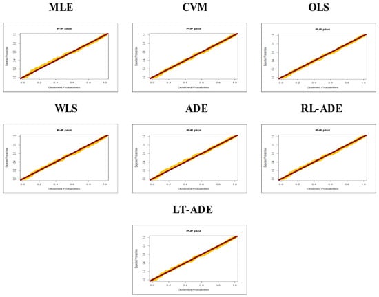
Figure 4. P-P plots for comparing estimation methods.

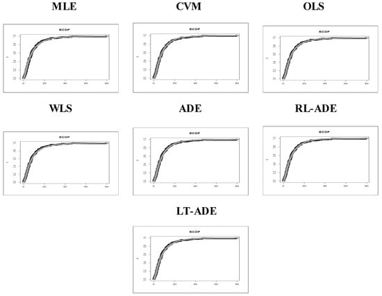
Figure 5. ECDF plots for comparing estimation methods.

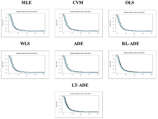
Figure 6. Kaplan–Meier estimation plots for comparing estimation methods.

5.2. For Comparing Competitive Models

An application is present, based on the data set of Cordeiro et al. [18], to show the flexibility of the TLE-NH model. We compare the TLE-NH model with some competitive models such as the Burr type-XII NH (BuXII-NH) ([19]), Lomax NH (Lx-NH) (Selim [19]), exponentiated exponential (Exp-Exp) beta exponential (B-Exp), Kumaraswamy exponential, TL-NH, inverse generalized power Weibull (IGPW) ([20]), inverse NH (I-NH), inverse Weibull (IW), inverse Rayleigh (IR), inverse exponential (IE) and NH distributions. Selecting the best model is performed using the estimated $-$log-likelihood, Akaike-Information-Criterion (AI$c$), Consistent-Akaike-Information-Criteria (CAI$c$), Bayesian-Information-Criterion (BI$c$), and Hannan–Quinn Information-Criterion (HQI$c$). This data has a unimodal HRF-shape. The results of this application are listed in Table 7 and Table 8. Table 7 lists the MLEs and the standard errors (SEs) for the asymmetric real data. Table 8 lists the statistics for the asymmetric real data. These results show that the TLE-NH distribution has the lowest AI$c$, CAI$c$, BI$c$ and HQI$c$ values among all the fitted models. Hence, it could be chosen as the best model under these criteria. Figure 7 gives the total time in test (TTT), box, quantile-quantile (QQ) and nonparametric Kernel density estimation (NKDE) plots for the real data. Figure 8 shows the estimated PDF (EPDF), ECDF, EHRF and Kaplan–Meier estimation plots. Clearly, the TLE-NH distribution provides a closer fit to the empirical functions. For this data, we have the following results: $E\left(Z\right)=$12.21692$,$ $V\left(Z\right)=$91.23032$,$ $S\left(Z\right)=$4.546743 and $K\left(Z\right)=$38.4308.

Table 7. The MLEs (SEs) for the real data.

Model	a	b	c
TLE-NH	0.3414	6.896	0.3875
	(0.3277)	(6.366)	(0.0347)
BuXII-NH	1.4763	0.11737	0.8259
	(0.2510)	(0.0215)	(0.00264)
B-Exp	1.1726	26.8142	0.0046
	(0.1312)	(0.6327)	(0.0006)
Kuw-Exp	1.4512	0.2816	0.4105
	(0.0240)	(0.0274)	(0.0154)
IGPW	0.4435	15.7165	1.2110
	(0.0482)	(4.8326)	(0.1023)
T-NH	(−1.0181)	0.43629
	(0.0505)	(0.01736)
TL-NH	3.1644		0.3161
	(0.3828)		(0.0165)
Lx-NH	0.1786		0.8259
	(0.01586)		(0.0027)
Exp-Exp	1.2179	0.1211
	(0.1488)	(0.0135)
NH	0.9227	0.1216
	(0.1515)	(0.0344)
IW	2.4311	0.7520
	(0.2192)	(0.0424)
INH	0.5064	10.5947
	(0.0480)	(2.3220)
IE	2.4847
	(0.2020)
IR	0.6174
	(0.0545)

Table 8. Statistics for the real data.

Model	$-$ℓ	$\mathbf{AI}\mathit{c}$$,\mathbf{CAI}\mathit{c}$$,\mathbf{BI}\mathit{c}$$,\mathbf{HQI}\mathit{c}$
TLE-NH	411.5920	829.1840, 829.3775, 837.7401, 832.6604
Kuw-Exp	412.4602	830.9204, 831.1139, 839.4765, 834.3968
Exp-Exp	413.0776	830.1552, 832.3487, 840.7113, 835.6316
B-Exp	413.3671	832.7342, 835.0594, 846.1423, 839.3693
NH	414.2255	832.4510, 832.5470, 838.1550, 834.7686
T-NH	414.4753	832.9505, 833.0465, 838.6546, 835.2681
BuXII-NH	414.5475	835.0949, 835.2885, 843.6510, 838.5713
TL-NH	415.0535	834.1069, 834.2029, 839.8110, 836.4245
Lx-NH	416.2293	836.4585, 836.5545, 842.1626, 838.7761
IGPW	426.9104	859.8194, 860.0135, 868.3751, 863.2964
INH	431.0593	866.1184, 866.2145, 871.8222, 868.4363
IW	444.0013	892.0022, 892.0986, 897.7060, 894.3192
IE	460.3826	922.7653, 922.7962, 925.6174, 923.9233
IR	774.3427	1550.683, 1550.715, 1553.535, 1551.842

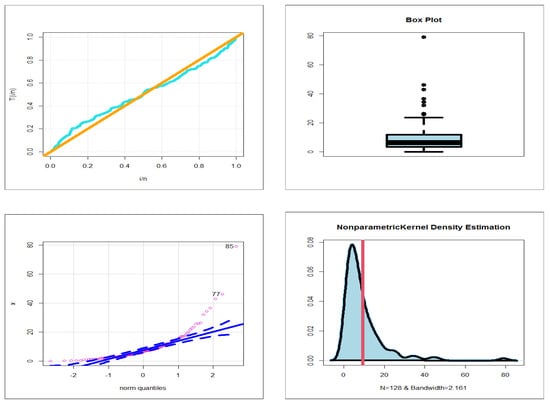
Figure 7. The TTT, box, QQ and NKDE plots for real data.

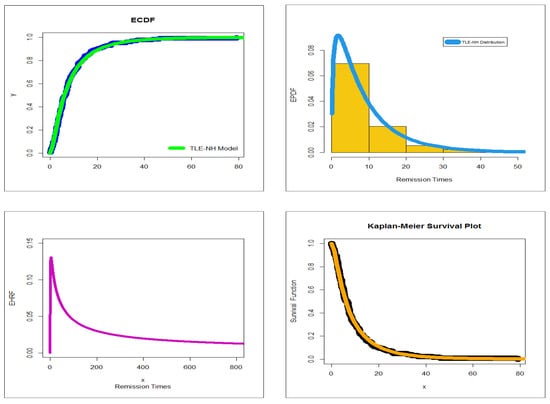
Figure 8. ECDF, EPDF, EHRF and Kaplan–Meier estimation plots.

6. Conclusions

In this paper, we have introduced a new flexible extension to the Nadarajah and Haghighi model called the Topp–Leone exponentiated Nadarajah and Haghighi model (TLE-NH). The PDF of the TLE-NH model can be expressed as a simple linear representation of the exponentiated NH density. Some of its statistical properties have been derived and studied in detail. The HRF can take different shapes, such as constant, increasing-constant, decreasing-constant, bathtub, upside down and upside down-U, which make the TLE-NH model able to analyze different types of data sets in various fields. Moreover, the TLE-NH model can be utilized to discuss both negatively and positively skewed data. The model parameters have been estimated by utilizing various estimation methods. Monte Carlo simulation experiments have been performed to compare the estimation methods. Finally, a real data set is analyzed for illustrating the flexibility of the proposed model, and it is found that the TLE-NH model showed its superiority in modeling the real data set.

References

- Nadarajah, S.; Haghighi, F. An extension of the exponential distribution. Statistics 2011, 45, 543–558. [Google Scholar] [CrossRef]
- Lemonte, A.J.; Cordeiro, G.M.; Moreno-Arenas, G. A new useful three-parameter extension of the exponential distribution. Statistics 2016, 50, 312–337. [Google Scholar] [CrossRef]
- Ortega, E.M.; Lemonte, A.J.; Silva, G.O.; Cordeiro, G.M. New flexible models generated by gamma random variables for lifetime modeling. J. Appl. Stat. 2015, 42, 2159–2179. [Google Scholar] [CrossRef]
- Ahmed, A.; Muhammed, H.Z.; Elbatal, I. A new class of extension exponential distribution. Int. J. Appl. Math. Sci. 2015, 8, 13–30. [Google Scholar]
- Lima, S.R.L. The Half Normal Generalized Family and Kummaraswamy Nadarajah Haghighi Distribution. Master’s Thesis, Universidade Federal de Pernumbuco, Recife, Brazil, 2015. [Google Scholar]
- El Damcese, M.A.; Ramadan, D.A. Studies on Properties and Estimation Problems for Modified Extension of Exponential Distribution. Int. J. Comput. Appl. 2015, 2015, 125. [Google Scholar] [CrossRef][Green Version]
- Lemonte, A.J. A new exponential-type distribution with constant, decreasing, increasing, upside-down bathtub and bathtub-shaped failure rate function. Comput. Stat. Data Anal. 2013, 62, 149–170. [Google Scholar] [CrossRef]
- Yousof, H.M.; Korkmaz, M.C. Topp-Leone Nadarajah Haghighi distribution: Mathematical properties and applications, International Journal of Applied Mathematics. J. Stat. Stat. Actuar. Sci. 2017, 2, 119–128. [Google Scholar]
- Dias, C.R.B.; Alizadeh, M.; Cordeiro, G.M. The beta Nadarajah-Haghighi distribution. Hacet. J. Math. Stat. 2018, 47, 1302–13203. [Google Scholar] [CrossRef]
- Tahir, M.H.; Cordeiro, G.M.; Ali, S.; Dey, S. The inverted Nadarajah-Haghighi distribution: Properties, estimation methods and applications. J. Stat. Comput. Simul. 2019, 88, 2775–2798. [Google Scholar] [CrossRef]
- Pena-Ramirez, F.A.; Guerra, R.R.; Cordeiro, G.M. The Nadarajah-Haghighi Lindley distribution. Acad Bras Cienc. 2019, 91, 1–20. [Google Scholar] [CrossRef]
- Maciak, M.; Okhrin, O.; Pešta, M. Infinitely stochastic micro reserving. Insur. Math. Econ. 2021, 100, 30–58. [Google Scholar] [CrossRef]
- Gijbels, I.; Omelka, M.; Pešta, M.; Veraverbeke, N. Score tests for covariate effects in conditional copulas. J. Multivar. Anal. 2017, 159, 111–133. [Google Scholar] [CrossRef]
- Eliwa, M.S.; Altun, E.; Alhussain, Z.A.; Ahmed, E.A.; Salah, M.M.; Ahmed, H.H.; El-Morshedy, M. A new one-parameter lifetime distribution and its regression model with applications. PLoS ONE 2021, 16, e0246969. [Google Scholar] [CrossRef] [PubMed]
- El-Morshedy, M.; Eliwa, M.S.; Altun, E. Discrete Burr-Hatke distribution with properties, estimation methods and regression model. IEEE Access 2020, 8, 74359–74370. [Google Scholar] [CrossRef]
- Hamedani, G.G.; Korkmaz, M.C.; Butt, N.S.; Yousof, H.M. The Type I Quasi Lambert Family: Properties, Characterizations and Different Estimation Methods. Pak. J. Stat. Oper. Res. 2021, 17, 545–558. [Google Scholar] [CrossRef]
- Elgohari, H.; Ibrahim, M.; Yousof, H.M. A New Probability Distribution for Modeling Failure and Service Times: Properties, Copulas and Various Estimation Methods. Stat. Optim. Inf. Comput. 2021, 8, 555–586. [Google Scholar] [CrossRef]
- Lee, E.T.; Wang, J. Statistical Methods for Survival Data Analysis; John Wiley & Sons: New York, NY, USA, 2003; Volume 476. [Google Scholar]
- Cordeiro, G.M.; Yousof, H.M.; Ramires, T.G.; Ortega, E.M. The Burr XII system of densities: Properties, regression model and applications. J. Stat. Comput. Simul. 2018, 88, 432–456. [Google Scholar] [CrossRef]
- Selim, M.A. Some theoretical and computational aspects of the inverse generalized power Weibull distribution. J. Data Sci. 2019, 17, 742–755. [Google Scholar] [CrossRef]
Publisher’s Note: MDPI stays neutral with regard to jurisdictional claims in published maps and institutional affiliations. |
© 2021 by the authors. Licensee MDPI, Basel, Switzerland. This article is an open access article distributed under the terms and conditions of the Creative Commons Attribution (CC BY) license (https://creativecommons.org/licenses/by/4.0/).