Cumulants of Multivariate Symmetric and Skew Symmetric Distributions

Abstract

This paper provides a systematic and comprehensive treatment for obtaining general expressions of any order, for the moments and cumulants of spherically and elliptically symmetric multivariate distributions; results for the case of multivariate t-distribution and related skew-t distribution are discussed in some detail.

1. Introduction

This paper provides a systematic treatment and derivation of moments and cumulants of any order for spherically as well as elliptically symmetric multivariate distributions. Expressions for the multivariate t-distribution and the related skew-t distribution are considered in detail. Our approach exploits the stochastic representation of such random variables in terms of the so-called generating variate and its uniform-distribution (Uniform) base in the appropriate dimension.

It is well known that the problem of representing the structure of higher-order cumulants of multivariate distributions is rather messy. In this paper, we present an approach based on a vectorization of cumulants which leads to a natural and intuitive way to obtain multivariate moments and cumulants of any order; we make the point that this provides the simplest way to deal with this issue.

We note that [1] provides formulae for cumulants in terms of matrices; however, retaining a matrix structure for all higher-order cumulants leads to high-dimensional matrices with special symmetric structures which are quite hard to follow notionally and computationally. Ref. [2] provides quite an elegant approach using tensor methods; however, tensor methods are not very well known and computationally not so simple.

The method discussed here is based on relatively simple calculus. Although the tensor product of Euclidean vectors is not commutative, it has the advantage of permutation equivalence and allows one to obtain general results for cumulants and moments of any order, as it will be demonstrated in this paper, where general formulae, suitable for algorithmic implementation through a computer software, will be provided. Methods based on a matrix approach do not provide this type of result; see also [3], which goes as far as the sixth-order moment matrices, whereas there is no such limitation in our derivations and our results. For further discussion, one can see also [4,5].

The primary contributions of this paper may be summarized as: (a) providing formulae, valid for any order, for vectorized cumulants and moments of multivariate spherical and elliptically symmetric distributions; matrix structures can be readily obtained from these expressions; some examples are provided in Section 4; (b) introduce the so-called marginal moment and cumulant parameters for multivariate spherical and elliptically symmetric distributions—providing an extension of the results discussed in [6]; (c) provide formulae for all-order moments and cumulants for multivariate t and skew-symmetric t-distributions; results of this type, as far as we know, are not available in the literature.

As is well known, cumulants play a key role in several areas of multivariate statistics: from the earliest applications in estimation and testing to fields such as signal detection, clustering, invariant coordinate selection, projection pursuit, time series modelling, pricing and portfolio analysis. See, for example, [7,8,9,10,11,12,13,14,15,16,17,18,19,20,21,22,23,24,25,26,27,28,29]. Higher-order cumulants going beyond the third and fourth order are typically needed to obtain the asymptotic properties of various statistics discussed in the aforementioned papers; for instance, ref. [30] provides general expressions for covariances of cumulants of the third and fourth order, requiring several higher-order cumulants. We believe that the expressions for higher-order cumulants for the models presented here open the door for such explorations in these areas.

In this paper, we will also go beyond such spherically and elliptically symmetric models, and obtain general expressions for the cumulants of skew-symmetric distributions such as the skew-t (see [31]). In particular, ref. [32] provides some specific analytical properties of skew-symmetric distributions. Further discussion on these distributions and their applications can be found in [33,34,35].

To formally introduce the problem, consider a random vector $\mathbf{X}$ in d-dimensions, with mean vector $\mu$ and covariance matrix $\Sigma$, $\lambda$ is a d-vector of real constants; let ${\varphi }_{\mathbf{X}}\left(\lambda \right)$ and ${\psi }_{\mathbf{X}}\left(\lambda \right)=log{\varphi }_{\mathbf{X}}\left(\lambda \right)$ denote, respectively, the characteristic function and the cumulant-generating function of $\mathbf{X}$.

With the symbol ⊗ denoting the Kronecker product, consider the operator $D_{\lambda }^{\otimes }$, which we refer to as the T-derivative; see [36] for details. For any function $\varphi \left(\lambda \right)$, the T-derivative is defined as

$$D_{\lambda }^{\otimes }\varphi \left(\lambda \right)=vec\left({\left(\frac{\partial \varphi \left(\lambda \right)}{\partial {\lambda }^{\top }}\right)}^{\top }\right)=\varphi \left(\lambda \right)\otimes \frac{\partial }{\partial \lambda }.$$

If $\varphi$ is k-times differentiable, with its k-th T-derivative $D_{\lambda }^{\otimes k}\varphi \left(\lambda \right)=D_{\lambda }^{\otimes }\left(D_{\lambda }^{\otimes k-1}\varphi \left(\lambda \right)\right),$ then the k-th order cumulant of the vector $\mathbf{X}$ is obtained as

$${\mathbf{\kappa }}_{\mathbf{X},k}^{\otimes }={\underline{Cum}}_k\left(\mathbf{X}\right)={(-\mathrm{i})}^k{D}_{\lambda }^{\otimes k}{\psi }_{\mathbf{X}}\left(\lambda \right){|}_{\lambda =0}.$$

(1)

Note that ${\underline{Cum}}_k\left(\mathbf{X}\right)$ is a vector of dimension $d^k$ that contains all possible cumulants of order k formed by $X_1,\cdots ,X_d$. For example, in Equation (1), one has ${\mathbf{\kappa }}_{\mathbf{X},2}=vec\Sigma$.

Throughout this paper, $\mathbb{N}$ is used for the set of natural numbers, $n!!$ for the double (semi-) factorial (see the reference [37]-Common Notations and Definitions) and ${\left(d\right)}_m=\Gamma (d+m)/\Gamma \left(d\right)$ for the Pochhammer symbol (see [37] 5.2.5), known also as the rising or ascending factorial. We will also denote

$$G_m\left(p\right)=\frac{\Gamma \left(\left(p+m\right)/2\right)}{\Gamma \left(p/2\right)},$$

(2)

so that $G_{2m}\left(p\right)={(p/2)}_m$. Finally, for any matrix $\mathbf{A}$, recall ${vec}^{\otimes m}\mathbf{A}={\left(vec\mathbf{A}\right)}^{\otimes m}$.

The paper is organized as follows. Section 2 discusses moments and cumulants of spherical and elliptically symmetric multivariate distributions; details on marginal moments and moment- and cumulant-parameters are provided. Section 3 considers the special case of multivariate t-distribution and discusses its extension to the skew-t distribution. Section 4 presents some applications and examples which are aimed mainly at providing evidence of the correctness of the formulae provided rather than providing simulations on estimation or testing. The proofs are collected in a separate section at the end, viz. Section 5.

2. Spherical and Elliptically Symmetric Distributions

For a comprehensive discussion of spherically and elliptically symmetric multivariate distributions, one may refer to the book by [38]. Other book-level discussions can be found, for instance, in [1,39,40]. General formulae for moments and kurtosis parameters are discussed in [6,41], among others.

A random variate $\mathbf{W}$ is spherically distributed if its distribution is invariant under rotations of ${\mathbb{R}}^d$, which is equivalent to having the stochastic representation

$$\mathbf{W}=R\mathbf{U},$$

(3)

where R is a non-negative random variable and $\mathbf{U}$ is a uniform random d-vector on the sphere ${\mathbb{S}}_{d-1}$, which is independent of R (see Theorem 2.5, [38]). The random variable R is called the generating variate, with the generating distribution F, and the random vector $\mathbf{U}$ is the uniform base of the spherical distribution. The characteristic function of $\mathbf{W}$ can then be written in the form ${\varphi }_{\mathbf{W}}\left(\lambda \right)=g\left({\lambda }^{⊺}\lambda \right)$ in terms of a given a function g, called the characteristic generator. An elliptically symmetric random variable $\mathbf{X}\in E_d\left(\mu ,\Sigma ,g\right)$ is defined by a location-scale extension of $\mathbf{W}$ so that it can be represented in the form

$$\mathbf{X}=\mu +{\Sigma }^{1/2}\mathbf{W}$$

(4)

where $\mu \in {\mathbb{R}}^d$, $\Sigma$ is a variance-covariance matrix and $\mathbf{W}$ is spherically distributed. The cumulants of $\mathbf{X}$ are just the cumulants of $\mathbf{W}$ multiplied by a constant, except for the mean, which is given by $E\mathbf{X}={\underline{Cum}}_1\left(\mathbf{X}\right)=\mu$. For $m\ge 1$

$${\underline{Cum}}_{2m}\left(\mathbf{X}\right)={\left({\Sigma }^{1/2}\right)}^{\otimes 2m}{\underline{Cum}}_{2m}\left(\mathbf{W}\right),\mathrm{and}{\underline{Cum}}_{2m+1}\left(\mathbf{X}\right)=0.$$

(5)

Let ${\psi }_{\mathbf{W}}\left(\lambda \right)=log{\varphi }_{\mathbf{W}}\left(\lambda \right)=logg\left({\lambda }^{⊺}\lambda \right)$ be the cumulant-generating function of $\mathbf{W}$. Consider the series expansions

$${\varphi }_{\mathbf{W}}\left(\lambda \right)=g\left({\lambda }^{⊺}\lambda \right)=\sum _{j=1}^{\infty }{\mu }_j^{\top \otimes }\frac{i^j}{j!}{\lambda }^{\otimes j}\mathrm{and}{\psi }_{\mathbf{W}}\left(\lambda \right)=\sum _{j=1}^{\infty }\frac{{\mathrm{i}}^j}{j!}{\mathbf{\kappa }}_{\mathbf{W},j}^{\otimes \top }{\lambda }^{\otimes j},$$

(6)

which lead to expressions for the moments and cumulants of $\mathbf{W}$ expressed through the T-derivative of the characteristic and log-characteristic generator functions as

$${\mu }_j^{\otimes }={\left.{(-\mathrm{i})}^j{D}_{\lambda }^{\otimes j}{\varphi }_{\mathbf{W}}\left(\lambda \right)\right|}_{\lambda =0}\mathrm{and}{\mathbf{\kappa }}_{\mathbf{W},j}^{\otimes }={\left.{(-\mathrm{i})}^j{D}_{\lambda }^{\otimes j}logg\left({\lambda }^{⊺}\lambda \right)\right|}_{\lambda =0}.$$

(7)

The relationship between the distribution F of R and g is given through the characteristic function of the uniform distribution on the sphere (see [38], Theorem 2.2, p. 29).

Using the stochastic representation (3) of $\mathbf{W}$, cumulants can be calculated either via the generator function g, or the distribution of the generating variate R. We first start with using the generator function g for deriving the cumulants of $\mathbf{W}$. Since the characteristic generator g is a function of one variable and represents the characteristic function at ${\lambda }^{⊺}\lambda$, the series expansion of g and $f=logg$ include ${\left(-1\right)}^j$ instead of ${\left(i\right)}^j$ and we have

$$g\left(u\right)=\sum _{j=1}^{\infty }\frac{{\left(-1\right)}^j}{j!}{g}_j{u}^j\mathrm{and}f\left(u\right)=\sum _{j=1}^{\infty }{f}_j\frac{{\left(-1\right)}^j}{j!}{u}^j,$$

(8)

with the coefficients $g_j={\left(-1\right)}^j{g}^{\left(j\right)}\left(0\right)$ and $f_j={\left(-1\right)}^j{f}^{\left(j\right)}\left(0\right)$. To introduce a specific notation, let us denote the generator moment by ${\nu }_k={\left(-1\right)}^k{g}^{\left(k\right)}\left(0\right)$ and the corresponding generator cumulant by ${\zeta }_k={\left(-1\right)}^k{f}^{\left(k\right)}\left(0\right)$.

Although neither the generator moments nor its cumulants correspond to the moments and cumulants of a random variate, the generator cumulants can be expressed in terms of the generator moments (and vice versa) via Faà di Bruno’s Formula, which says:

$${\zeta }_k=\sum _{r=1}^k{(-1)}^{r-1}(r-1)!\sum _{\Sigma {\ell }_j=r,\Sigma j{\ell }_j=k}\frac{k!}{{\prod }_{j=1}^k{\ell }_j!}\prod _{j=1}^k{\left(\frac{{\nu }_j}{j!}\right)}^{{\ell }_j},$$

(9)

where the second sum is taken over all sequences (types) $\ell =\left({\ell }_1,\dots ,{\ell }_k\right)$, ${\ell }_j\ge 0$ such that ${\sum }_{{\ell }_j\in \ell }{\ell }_j=r$ and ${\sum }_{{\ell }_j\in \ell }j{\ell }_j=k$.

2.1. Marginal Moments and Cumulants

If one takes the derivatives of ${\varphi }_{W_j}\left({\lambda }_j\right)=g\left({\lambda }_j^2\right)$, at ${\lambda }_j=\left(0,\cdots ,{\lambda }_j,\cdots ,0\right)$, it is readily seen that these derivatives do not depend on j; also, the odd moments can be seen to be zero (see, e.g., [6]).

The following theorem (which is proven in Section 5) establishes the connection between (i) the moments of $W_j$ and the generator moments, as well as (ii) cumulants of $W_j$ and the generator cumulants.

Theorem 1.

Let $m\in \mathbb{N}$ and, in (3), assume $E\left(R^m\right)<\infty$. Define ${\mu }_{W,m}$ and ${\kappa }_{W,m}$ as the $m^{th}$ order moment and cumulant of $W_j$, while ${\nu }_m$ and ${\zeta }_m$ denote the generator moment and generator cumulant of the $m^{th}$ order. Then, the odd moments ${\mu }_{W,2m+1}=E{W}_j^{2m+1}$ of $W_j$ are all zero and the even ones are

$${\mu }_{W,2m}=2^m\left(2m-1\right)!!{\nu }_m=\frac{\left(2m\right)!}{m!}{\nu }_m.$$

(10)

Again, the odd cumulants ${\kappa }_{W,2m+1}$ of $W_j$ are zero as well, and the even ones are given by

$${\kappa }_{W,2m}=2^m\left(2m-1\right)!!{\zeta }_m=\frac{\left(2m\right)!}{m!}{\zeta }_m.$$

(11)

Further, the even cumulants can be expressed in terms of the generator moments as

$${\kappa }_{W,2m}=2^m\left(2m-1\right)!!\sum _{r=1}^m{(-1)}^{r-1}(r-1)!\sum _{\Sigma {\ell }_j=r,\Sigma j{\ell }_j=m}\frac{m!}{{\prod }_{j=1}^{\ell }{\ell }_j!}\prod _{j=1}^{\ell }{\left(\frac{{\nu }_j}{j!}\right)}^{{\ell }_j}$$

(12)

where the second sum is taken over all sequences $\ell =\left({\ell }_1,\dots ,{\ell }_{\ell }\right)$, ${\ell }_j\ge 0$, satisfying ${\sum }_{j=1}^{\ell }{\ell }_j=r$ and ${\sum }_{j=1}^{\ell }j{\ell }_j=m$.

Example 1.

Applying Theorem 1 in particular for $m=4,6,8$ yields

$$\begin{array}{cc}\hfill {\kappa }_{W,4}& ={\mu }_{W,4}-3{\mu }_{W,2}^2=12{\nu }_2-12{\nu }_1^2=12\left({\nu }_2-{\nu }_1^2\right),\hfill \\ \hfill {\kappa }_{W,6}& =2^{3}5!!\left({\nu }_3-3{\nu }_2{\nu }_1+2{\nu }_1^3\right)\hfill \\ \hfill {\kappa }_{W,8}& =2^{4}7!!\left({\nu }_4-4{\nu }_3{\nu }_1-3{\nu }_2^2+12{\nu }_2{\nu }_1^2-6{\nu }_1^4\right),\hfill \end{array}$$

2.1.1. Moment and Cumulant Parameters

The fourth-order cumulant of the standardized $W_j$ for each entry $W_j$, usually called kurtosis, has the form

$$\frac{{\kappa }_{W,4}}{{\kappa }_{W,2}^2}=3\frac{{\nu }_2-{\nu }_1^2}{{\nu }_1^2}=3\frac{{\zeta }_2}{{\nu }_1^2}={Cum}_4\left(\frac{W_j}{\sqrt{2{\nu }_1}}\right).$$

(13)

In the above formula, we observe two quantities: one is the kurtosis (standardized generator cumulant since ${\nu }_1={\zeta }_1$), i.e.,

$${\tilde{\kappa }}_2=\frac{{\zeta }_2}{{\nu }_1^2},$$

(14)

and the other one is ${\tilde{\mu }}_2=({\nu }_2-{\nu }_1^2)/{\nu }_1^2={\nu }_2/{\nu }_1^2-1,$ which contains the standardized generator moment ${\nu }_2/{\nu }_1^2$. Both quantities ${\tilde{\mu }}_2$ and ${\tilde{\kappa }}_2$ have the same value (see Equation (13)). The kurtosis ${\tilde{\kappa }}_2$ is sometimes called the kurtosis parameter (see, for instance, [39]). Observe that the parameter ${\tilde{\mu }}_2$ depends on the generator moment of the standardized variate only, so it can be called the moment parameter as in [6].

More generally, for $m\ge 1$, define the moment parameters and the cumulant parameters, respectively, as

$${\tilde{\mu }}_m=\frac{{\nu }_m}{{\nu }_1^m}-1\mathrm{and}{\tilde{\kappa }}_m=\frac{{\zeta }_m}{{\nu }_1^m}$$

(15)

The following normalized cumulants of $W_j$, where cumulant parameters ${\tilde{\kappa }}_m$ are expressed in terms of moment parameters ${\tilde{\mu }}_m$, connect our different notations

$$\begin{array}{cc}\hfill {Cum}_2\left(\frac{W_j}{\sqrt{2{\nu }_1}}\right)& =1,\hfill \\ \hfill {Cum}_4\left(\frac{W_j}{\sqrt{2{\nu }_1}}\right)& =3!!{\tilde{\kappa }}_2=3!!{\tilde{\mu }}_2,\hfill \\ \hfill {Cum}_6\left(\frac{W_j}{\sqrt{2{\nu }_1}}\right)& =5!!{\tilde{\kappa }}_3=5!!\left({\tilde{\mu }}_3-3{\tilde{\mu }}_2\right),\hfill \\ \hfill {Cum}_8\left(\frac{W_j}{\sqrt{2{\nu }_1}}\right)& =7!!{\tilde{\kappa }}_4=7!!\left({\tilde{\mu }}_4-4{\tilde{\mu }}_3-3{\tilde{\mu }}_2^2+6{\tilde{\mu }}_2\right).\hfill \end{array}$$

(16)

As will be seen in Section 3, using moment and cumulant parameters reduces the number of parameters for a spherically distributed random variate $\mathbf{W}$ significantly, while the number of characteristics is halved for an elliptically symmetric distribution. The cumulant parameters ${\tilde{\kappa }}_m$ can be expressed in terms of moment parameters ${\tilde{\mu }}_m$ in higher orders as well.

Corollary 1.

Under the assumptions of Theorem 1, the moments of standardized $W_j$ are zero for odd orders and

$$E{\left(\frac{W_j}{\sqrt{2{\nu }_1}}\right)}^{2m}=\frac{{\mu }_{W,2m}}{{\left(2{\nu }_1\right)}^m}=\left(2m-1\right)!!\left({\tilde{\mu }}_m+1\right),$$

for even orders, where ${\tilde{\mu }}_m$ is the moment parameter defined in (15). The cumulants of standardized $W_j$ are zero for odd orders and

$${Cum}_{2m}\left(\frac{W_j}{\sqrt{2{\nu }_1}}\right)=\left(2m-1\right)!!{\tilde{\kappa }}_m,$$

for even orders, where ${\tilde{\kappa }}_m$ is the cumulant parameter (15), such that

$${\tilde{\kappa }}_m=\sum _{r=1}^m{(-1)}^{r-1}(r-1)!\sum _{\Sigma {\ell }_j=r,\Sigma j{\ell }_j=m}\frac{m!}{{\prod }_{j=1}^{\ell }{\ell }_j!}\prod _{j=1}^{\ell }{\left(\frac{{\tilde{\mu }}_j+1}{j!}\right)}^{{\ell }_j}.$$

(17)

Formula (17) is valid for all $m\ge 1$, since, as seen earlier, ${\tilde{\mu }}_1=0$ and ${\tilde{\kappa }}_1=1$.

2.1.2. Using the Representation RU

We now turn to the stochastic representation (3) and consider the scalar variable case $W_j=R{U}_j$. We first explore the even order moments ${\mu }_{W,2m}={\mu }_{R,2m}.{\mu }_{U_j,2m}.$ Using the result on the even-order moments $E{U}_j^{2m}$ as given in Lemma 1 in [29], we get

$${\mu }_{W,2m}=\frac{{\mu }_{R,2m}}{2^m{\left(d/2\right)}_m}\left(2m-1\right)!!.$$

(18)

This result in combination with Equation (10) lets us express the generator moment ${\nu }_m$ in terms of the moment of the generating variate R as

$${\nu }_m={\mu }_{R,2m}\frac{m!}{\left(2m\right)!}\frac{\left(2m\right)!}{2^{2m}m!{\left(d/2\right)}_m}=\frac{{\mu }_{R,2m}}{2^{2m}{\left(d/2\right)}_m}.$$

(19)

Alternatively, in terms of moments of W, this becomes

$${\nu }_m=\frac{{\mu }_{W,2m}}{2^m\left(2m-1\right)!!}.$$

(20)

The dependence of moment parameter ${\tilde{\mu }}_m$ on the moment of the generating variate R follows directly from the definition of ${\tilde{\mu }}_m$ and the above expression

$${\tilde{\mu }}_m=\frac{{\nu }_m}{{\nu }_1^m}-1=\frac{{\left(d/2\right)}^m{\mu }_{R,2m}}{{\left(d/2\right)}_m{\mu }_{R,2}^m}-1.$$

(21)

If $U_j$ is one component of the vector $\mathbf{U}$, then the stochastic representation (3) of $\mathbf{W}$ implies $W_j=R{U}_j$. Therefore, the cumulants of $W_j$ can be expressed either by the moments or the cumulants of R. Thus, the cumulants of $W_j$ are connected to the cumulants of R in general. Since the cumulant ${Cum}_n\left(W\right)$ is an $n^{th}$ order cumulant of the product $R{U}_1$ of two independent variates, a direct method for its calculation can be made using the conditional cumulants. Using this idea provides the following.

Example 2.

Consider, e.g., the fourth-order cumulant ${\kappa }_{W,4}={\kappa }_{R{U}_1,4}$ of say $W_1$ (since all $W_j$ have identical distributions). Applying the formula for cumulants via moments, and using the independence of R and $U_j$, one obtains

$${\kappa }_{W,4}={\mu }_{R,4}{\mu }_{U_1,4}-3{\left({\mu }_{R,2}{\mu }_{U_1,2}\right)}^2.$$

Now, using particular values for moments of $U_j$ gives

$${\kappa }_{W,4}=\frac{3}{d\left(d+2\right)}\left({\kappa }_{R^2,2}+{\kappa }_{R^2,1}^2\right)-\frac{3}{d^2}{\kappa }_{R^2,1}^2=-\frac{6}{d^2\left(d+2\right)}{\kappa }_{R^2,1}^2+\frac{3}{d\left(d+2\right)}{\kappa }_{R^2,2}.$$

(22)

Lemma 1.

Let $n\in \mathbb{N}$ and, in (3), assume $E\left(R^n\right)<\infty$. The even-order cumulants of a component $W_j$ of a spherically distributed random variate $\mathbf{W}$ are given in terms of generating variate R as follows

$${\kappa }_{W,2n}=\left(2n\right)!\sum _{r=1}^{2n}\sum _{\begin{array}{c}\Sigma {\ell }_j=r,\Sigma j{\ell }_j=n\\ jiseven\end{array}}{Cum}_r\left(R_{\left\{{\ell }_1\right\}},R_{\left\{{\ell }_2\right\}}^2,\dots ,R_{\left\{{\ell }_n\right\}}^n\right)\prod _{j=1}^{n-r+1}\frac{1}{{\ell }_j!}{\left(\frac{{\kappa }_{U_1,j}}{j!}\right)}^{{\ell }_j},$$

(23)

where the summation is taken over all even-order cumulants of $U_1$, since the odd orders are zero and where $R_{\left\{{\ell }_j\right\}}^j$ corresponds to the block with cardinality ${\ell }_j$, which includes power $R^j$ only (it implies listing $R^j$ consecutively ${\ell }_j$ times).

Here, the cumulants ${\kappa }_{U_1,j}$ of $U_1$ are involved, which can be evaluated explicitly in particular cases to obtain the formula for ${\kappa }_{W_1,2n}$.

Example 3.

Consider the fourth-order cumulant ${\kappa }_{W,4}={\kappa }_{R{U}_1,4}$ of $W_j$, say. Applying the formula to cumulant (23) gives

$${\kappa }_{R{U}_1,4}={\kappa }_{R^4,1}{\kappa }_{U_1,4}+3{\kappa }_{R^2,2}{\kappa }_{U_1,2}^2.$$

(24)

Next, obtain the cumulants of $U_1$ from the moments

$$\begin{array}{ccc}\hfill {\mu }_{U_1,4}& =& \frac{3}{d\left(d+2\right)},\hfill \\ \hfill {\kappa }_{U_1,2}^2& =& {\mu }_{U_1,2}=1/d,\hfill \\ \hfill {\kappa }_{U_1,4}& =& {\mu }_{U_1,4}-3{\mu }_{U_1,2}^2=\frac{3}{d\left(d+2\right)}-\frac{3}{d^2}=-\frac{6}{d^2\left(d+2\right)}.\hfill \end{array}$$

Finally, plugging these into (24) and using (22), one obtains

$${\kappa }_{R{U}_1,4}=-\frac{6}{d^2\left(d+2\right)}{\kappa }_{R^4,1}+3\frac{1}{d^2}{\kappa }_{R^2,2}.$$

(25)

2.2. Multivariate Moments and Cumulants

Rewriting the characteristic function using the series expansion of $g\left(u\right)$ given in (8), one obtains

$${\varphi }_{\mathbf{W}}\left(\lambda \right)=g\left({\lambda }^{⊺}\lambda \right)=\sum _{j=1}^{\infty }\frac{{\left(-1\right)}^j{g}_j}{j!}\left({\lambda }^{⊺}\lambda \right).$$

The moments can be calculated using Equation (7) as follows

$${\left.{(-\mathrm{i})}^k{D}_{\lambda }^{\otimes k}{\varphi }_{\mathbf{W}}\left(\lambda \right)\right|}_{\lambda =0}={(-\mathrm{i})}^k\sum _{j=1}^{\infty }\frac{{\left(-1\right)}^j{g}_j}{j!}{\left.D_{\lambda }^{\otimes k}{\left({\lambda }^{⊺}\lambda \right)}^j\right|}_{\lambda =0}.$$

Observe that

$${\mu }_k^{\otimes }={\left.{(-\mathrm{i})}^k{D}_{\lambda }^{\otimes k}{\varphi }_{\mathbf{W}}\left(\lambda \right)\right|}_{\lambda =0}={\left.{(-\mathrm{i})}^k\sum _{j=1}^{\infty }\frac{{\left(-1\right)}^j{g}_j}{j!}{D}_{\lambda }^{\otimes k}{\left({\lambda }^{⊺}\lambda \right)}^j\right|}_{\lambda =0}=\left\{\begin{array}{ccc}0& \mathrm{if}& 2j\ne k,\\ {\displaystyle \frac{1}{j!}}{g}_j{\mathbf{c}}_j& \mathrm{if}& 2j=k,\end{array}\right.$$

and the vector ${\mathbf{c}}_j$ does not depend on g. Using $g_j={\left(-1\right)}^j{g}^{\left(j\right)}\left(0\right)={\nu }_j$, and ${\mathbf{c}}_j=D_{\lambda }^{\otimes 2j}{\left({\lambda }^{⊺}\lambda \right)}^j$, we have ${\mu }_{\mathbf{W},2m}^{\otimes }=\frac{{\nu }_m}{m!}{D}_{\lambda }^{\otimes 2m}{\left({\lambda }^{⊺}\lambda \right)}^m$. This derivation provides the connection between the generator moments and the marginal moments in (10), by using which, one obtains

$${\mu }_{\mathbf{W},2m}^{\otimes }=\frac{{\mu }_{W_1,2m}}{m!2^m\left(2m-1\right)!!}{D}_{\lambda }^{\otimes 2m}{\left({\lambda }^{⊺}\lambda \right)}^m=\frac{{\mu }_{W_1,2m}}{\left(2m\right)!}{D}_{\lambda }^{\otimes 2m}{\left({\lambda }^{⊺}\lambda \right)}^m.$$

The same argument applies to the cumulant generator function ${\psi }_{\mathbf{W}}\left(\lambda \right)=log{\varphi }_{\mathbf{W}}\left(\lambda \right)$ with series expansion (8). Now, we obtain ${\kappa }_{2m}^{\otimes }={\zeta }_m/m!D_{\lambda }^{\otimes 2m}{\left({\lambda }^{⊺}\lambda \right)}^m$, and since ${\zeta }_m$ is connected to the $m^{th}$ cumulant of a component of $\mathbf{W}$ by (11), we get

$${\mathbf{\kappa }}_{\mathbf{W},2m}^{\otimes }=\frac{{\kappa }_{W,2m}}{2^{m}m!\left(2m-1\right)!!}{D}_{\lambda }^{\otimes 2m}{\left({\lambda }^{⊺}\lambda \right)}^m=\frac{{\kappa }_{W,2m}}{\left(2m\right)!}{D}_{\lambda }^{\otimes 2m}{\left({\lambda }^{⊺}\lambda \right)}^m.$$

Recall that ${\mathcal{K}}_{\left\{r|\ell \right\}}$ denotes particular partitions with size r and type ℓ. The above calculations are summarized in the following theorem, which has been stated without proof and used in [30]. One finds “commutator matrices”, which change the order of the tensor products according to a given permutation, very useful. (For a brief description of the commutator matrices and the symmetrizer, the reader is referred to Section 5.1).

Theorem 2.

Let $m\in \mathbb{N}$ and, in (3), assume $E\left(R^m\right)<\infty$. The moments and cumulants of odd orders of spherically distributed $\mathbf{W}$ are zero. The moments of even orders are given by

$${\mu }_{\mathbf{W},2m}^{\otimes }=\frac{{\mu }_{W,2m}}{\left(2m-1\right)!!}{\mathbf{L}}_{m_2}^{-1}{vec}^{\otimes m}{\mathbf{I}}_d={\mu }_{W,2m}{\mathbf{S}}_{d{\mathbf{1}}_{2m}}{vec}^{\otimes m}{\mathbf{I}}_d,$$

while the cumulants of even orders are

$${\mathbf{\kappa }}_{\mathbf{W},2m}^{\otimes }=\frac{{\kappa }_{W,2m}}{\left(2m-1\right)!!}{\mathbf{L}}_{m_2}^{-1}{vec}^{\otimes m}{\mathbf{I}}_d={\kappa }_{W,2m}{\mathbf{S}}_{d{\mathbf{1}}_{2m}}{vec}^{\otimes m}{\mathbf{I}}_d.$$

In terms of moment parameters, the standardized cumulants

$${\underline{Cum}}_{2m}\left({\Sigma }^{-1/2}\mathbf{W}\right)={\tilde{\kappa }}_m{\mathbf{L}}_{m_2}^{-1}{vec}^{\otimes m}{\mathbf{I}}_d,$$

(26)

where ${\Sigma }^{-1/2}=1/\sqrt{2{\nu }_1}{\mathbf{I}}_d$. Formula (17) shows that ${\tilde{\kappa }}_m$ is a polynomial in ${\tilde{\mu }}_k$, k = 2:m. We denote this polynomial by $a_m\left({\tilde{\mu }}_2\dots ,{\tilde{\mu }}_m\right)={\tilde{\kappa }}_m$, hence

$${\underline{Cum}}_{2m}\left({\Sigma }^{-1/2}\mathbf{W}\right)=a_m\left({\tilde{\mu }}_2\dots ,{\tilde{\mu }}_m\right){\mathbf{L}}_{m_2}^{-1}{vec}^{\otimes m}{\mathbf{I}}_d.$$

In particular, when $a_1=1$

$$a_m\left({\tilde{\mu }}_2,\dots ,{\tilde{\mu }}_m\right)=\left\{\begin{array}{cc}{\tilde{\mu }}_2,\hfill & m=2,\\ {\tilde{\mu }}_3-3{\tilde{\mu }}_2,\hfill & m=3,\\ {\tilde{\mu }}_4-4{\tilde{\mu }}_3-3{\tilde{\mu }}_2^2+6{\tilde{\mu }}_2,\hfill & m=4,\end{array}\right.$$

Remark 1.

Both higher-order moments ${\mu }_{\mathbf{W},2m}^{\otimes }$ and cumulants ${\mathbf{\kappa }}_{\mathbf{W},2m}^{\otimes }$ use a commutator matrix ${\mathbf{L}}_{m_2}^{-1}$ or a symmetrizer ${\mathbf{S}}_{d{\mathbf{1}}_{2m}}$; details are given in Section 5.1. Determining ${\mathbf{L}}_{m_2}^{-1}$ may be cumbersome although much lighter, from a computational point of view, than the actual calculation of the symmetrizer, which, for large dimensions d and order $2m$, is very time-, memory- and space- consuming. Alternatively, one can get an efficient calculation evaluating the $D_{\lambda }^{\otimes 2m}{\left({\lambda }^{⊺}\lambda \right)}^m$ by using the T-derivative step by step. For example,

$$D_{\lambda }^{\otimes 4}{\left({\lambda }^{⊺}\lambda \right)}^2=2^3\left({\mathbf{I}}_{d^4}+{\mathbf{K}}_{\left(3214\right)}^{-1}+{\mathbf{K}}_{\left(1324\right)}^{-1}\right){vec}^{\otimes 2}{\mathbf{I}}_d=2^3{\mathbf{L}}_{2_2}^{-1}{vec}^{\otimes 2}{\mathbf{I}}_d,$$

where 3 commutator matrices are included instead of the 24, which are necessary for obtaining ${\mathbf{S}}_{d{\mathbf{1}}_4}$. Further examples can be found in [30].

Remark 2.

Deriving $D_{\lambda }^{\otimes 6}{\left({\lambda }^{⊺}\lambda \right)}^3$ means finding 15 partitions ${\mathcal{K}}_{\left\{3|\ell \right\}}$, with size 3 and type $\ell =\left(0,3,0,0,0,0\right)$, i.e., splitting up the set 1:6 into three blocks, and each block contains two elements. The partitions are in canonical form and the corresponding commutator ${\mathbf{L}}_{3_2}^{-1}$ is listed in Section 4.1. The result is

$$D_{\lambda }^{\otimes 6}{\left({\lambda }^{⊺}\lambda \right)}^3=48{\mathbf{L}}_{3_2}^{-1}{vec}^{\otimes 3}{\mathbf{I}}_d.$$

Then, $E{\mathbf{W}}^{\otimes 2m}$ can be calculated directly from the expected values of the entries. The nonzero entries of $E{\mathbf{W}}^{\otimes 2m}$ are those where all terms in the product of entries of $\mathbf{W}$ have even degrees (cf. (18)).

Remark 3.

We compare the expected values of the entries of ${\mathbf{W}}^{\otimes 2m}$ to the expected values of those in ${\mathbf{Z}}^{\otimes 2m}$, where $\mathbf{Z}$ is a standard normally distributed variate. The nonzero entries of the expected value $E{\mathbf{Z}}^{\otimes 2m}$ are products with even powers such that

$$E\prod _{i=1}^d{Z}_i^{2k_i}=\prod _{i=1}^d\left(2k_i-1\right)!!,$$

where $\Sigma k_{1:d}=m$. At the same time, we have $E{\mathbf{Z}}^{\otimes 2m}=\left(2m-1\right)!!{\mathbf{S}}_{d{\mathbf{1}}_{2m}}{vec}^{\otimes m}{\mathbf{I}}_d.$ Comparing this to $E{\mathbf{W}}^{\otimes 2m}=E{W}_1^{2m}{\mathbf{S}}_{d{\mathbf{1}}_{2m}}{vec}^{\otimes m}{\mathbf{I}}_d,$ we conclude that the higher-order moments of an elliptic random vector $\mathbf{W}$ differ from the moments of a normal one $\mathbf{Z}$ only in the constant $E{W}_1^{2m}$. The major difference turns up in comparing the cumulants, since cumulants of order higher than 2 for $\mathbf{Z}$ are zero while the cumulants of $\mathbf{W}$ are

$${\underline{Cum}}_{2m}\left(\mathbf{W}\right)={Cum}_{2m}\left(W_1\right){\mathbf{S}}_{d{\mathbf{1}}_{2m}}{vec}^{\otimes m}{\mathbf{I}}_d.$$

Example 4.

If the generating variate R is Gamma distributed with parameters $\vartheta >0$, $\alpha >0$, then

$$E{R}^r=\frac{{\vartheta }^r\Gamma \left(\alpha +r\right)}{\Gamma \left(\alpha \right)},$$

and the kurtosis parameter ${\tilde{\kappa }}_2$ becomes

$$\begin{array}{cc}\hfill {\tilde{\kappa }}_2& =\left(\frac{d}{d+2}\frac{E{R}^4}{{\left(E{R}^2\right)}^2}-1\right)=\frac{d}{d+2}\frac{\Gamma \left(\alpha +4\right)\Gamma \left(\alpha \right)}{\Gamma {\left(\alpha +2\right)}^2}-1\hfill \\ \hfill & =\frac{d}{d+2}\left(\alpha +3\right)\left(\alpha +2\right)\frac{\Gamma \left(\alpha \right)}{\Gamma \left(\alpha +2\right)}-1=\frac{d}{d+2}\frac{\left(\alpha +3\right)\left(\alpha +2\right)}{\alpha \left(\alpha +1\right)}-1.\hfill \end{array}$$

3. Multivariate t and Skew-t Distributions

There have been several attempts to introduce asymmetry into multivariate distributions by “skewing” a given spherically or elliptically symmetric distribution such as the normal or a t-distribution. The multivariate skew-normal distribution was introduced by [42]; see also [43]. Ref. [44] derived the first four moments and discussed quadratic forms based on these; for further properties, see [45].

For the case of the multivariate skew-symmetric-t, we use the definition given in [31], which is different from that provided by [46]. Its moments were derived in [47]. For further discussion on these distributions and their applications, see [32,33,34,35].

3.1. Multivariate t-Distribution

The d-variate vector $\mathbf{W}$ is t-distributed, written as $\mathbf{W}\in M{t}_d\left(p,0,{\mathbf{I}}_d\right)$, if $\mathbf{W}=\sqrt{p}\mathbf{Z}/S$ where $\mathbf{Z}\in {\mathcal{N}}_d\left(0,{\mathbf{I}}_d\right)$ is standard normal, and $S^2$ is ${\chi }^2$ distributed with p degrees of freedom. See Example 2.5, Section 3.3.6, p. 85 [38], and p. 32. Such a random variable $\mathbf{W}\in M{t}_d\left(p,0,{\mathbf{I}}_d\right)$ is spherically distributed since it has the representation

$$\mathbf{W}=\sqrt{p}\frac{∥\mathbf{Z}∥}{S}\mathbf{Z}/∥\mathbf{Z}∥=R\mathbf{U},$$

(27)

where $R=\sqrt{p}∥\mathbf{Z}∥/S$ is the generating variate. We note that $R^2/d\in F\left(d,p\right)$ has an F-distribution with d and p degrees of freedom (cf. also [48]). Let $\mu \in {\mathbb{R}}^d$, and $\mathbf{A}$ is a $d\times d$ matrix; then, the linear transform $\mathbf{X}=\mu +{\mathbf{A}}^{⊺}\mathbf{W}$ will be considered as $\mathbf{X}\in M{t}_d\left(p,\mu ,\Omega \right)$, where $\Omega ={\mathbf{A}}^{⊺}\mathbf{A}$; hence, $\mathbf{X}$ is an elliptically symmetric random variable. The characteristic function of $\mathbf{X}$ is quite involved, and therefore we utilize the stochastic representation of $\mathbf{W}$ viz. (27), for deriving higher-order cumulants including skewness and kurtosis for $\mathbf{X}$. For the even-order moments of the generating variate R, i.e., the even-order moments of the F-distribution with d and p degrees of freedom, with $p>2m$, we have

$$\frac{E{R}^{2m}}{d^m}={\left(\frac{p}{d}\right)}^m\frac{\Gamma \left(d/2+m\right)\Gamma \left(p/2-m\right)}{\Gamma \left(d/2\right)\Gamma \left(p/2\right)}={\left(\frac{p}{d}\right)}^m{G}_{2m}\left(d\right)G_{-2m}\left(d\right),$$

so that

$${\mu }_{R,2m}=\frac{p^m{\left(d/2\right)}_m}{{\left(p/2-m+1\right)}_m}=\frac{p^m{\left(d/2\right)}_m}{{\left(1-p/2\right)}_m}=\frac{p^m{\left(d/2\right)}_m}{{\left(p/2-m\right)}_m}.$$

We also have the even-order moments of the components of uniform distribution (on sphere ${\mathbb{S}}_{d-1}$)

$${\mu }_{U_1,2m}=\frac{\left(2m-1\right)!!}{2^m{\left(d/2\right)}_m}.$$

These two quantities will provide us the moments of the components of $\mathbf{W}$ as

$${\mu }_{W,2m}={\mu }_{R,2m}{\mu }_{U_1,2m}=\frac{p^m{\left(d/2\right)}_m}{{\left(p/2-m\right)}_m}\frac{\left(2m-1\right)!!}{2^m{\left(d/2\right)}_m}=\frac{p^m\left(2m-1\right)!!}{2^m{\left(p/2-m\right)}_m}.$$

(28)

Recall that all entries of $\mathbf{W}$ have the same distribution so that one can use the notation W for the generic entry. The cumulants of even order of W can be calculated with the help of the cumulant parameters ${\tilde{\kappa }}_m$. Consider the moment parameters ${\tilde{\mu }}_m$ first, which is

$${\tilde{\mu }}_m=\frac{1}{\alpha \left(d,m\right)}\frac{{\mu }_{R,2m}}{{\mu }_{R,2}^m}-1=\frac{{\left(d/2\right)}^m}{{\left(d/2\right)}_m}\frac{p^m{\left(d/2\right)}_m}{{\left(p/2-m\right)}_m}{\left(\frac{p/2-1}{pd/2}\right)}^m-1=\frac{{\left(p/2-1\right)}^m}{{\left(p/2-m\right)}_m}-1,$$

(29)

(see Equation (21) for the moments of R). Then, the cumulant parameter ${\tilde{\kappa }}_m$ is calculated using the general expression (17). Theorem 2 then leads us to the following.

Lemma 2.

Let $p>2m$ and $\mathbf{W}$ be t-multivariate, $\mathbf{W}\in M{t}_d\left(p,0,{\mathbf{I}}_d\right)$, with dimension d and degrees of freedom p, then $E\mathbf{W}=0$, and both the moments and the cumulants with odd higher order are zero. The moments with even order are given by

$${\mu }_{\mathbf{W},2m}^{\otimes }=\frac{p^m}{2^m{\left(p/2-m\right)}_m}{\mathbf{L}}_{m_2}^{-1}{vec}^{\otimes m}{\mathbf{I}}_d.$$

The covariance matrix of $\mathbf{W}$ has the diagonal form $Var\mathbf{W}=\Sigma =\frac{p}{p-2}{\mathbf{I}}_d$ and the even-order standardized cumulants are

$${\underline{Cum}}_{2m}\left({\Sigma }^{-1/2}\mathbf{W}\right)={\tilde{\kappa }}_m{\mathbf{L}}_{m_2}^{-1}{vec}^{\otimes m}{\mathbf{I}}_d,$$

where the cumulant parameters ${\tilde{\kappa }}_m$ are given by the expression (17) and moment parameters in (29). In particular, this gives

$$\begin{array}{cc}\hfill {Cum}_2\left(\frac{W_j}{\sqrt{2{\nu }_1}}\right)& =1,\hfill \\ \hfill {Cum}_4\left(\frac{W_j}{\sqrt{2{\nu }_1}}\right)& =3!!\frac{2}{p-4},\hfill \\ \hfill {Cum}_6\left(\frac{W_j}{\sqrt{2{\nu }_1}}\right)& =5!!\frac{16}{\left(p-4\right)\left(p-6\right)}.\hfill \end{array}$$

(30)

3.2. Multivariate Skew-t Distribution

Let $\mathbf{V}$ be a d-dimensional multivariate skew-normal distribution, denoted by $\mathbf{V}\in S{N}_d\left(0,\Omega ,\alpha \right)$, and $S^2$ be an independently distributed ${\chi }^2$ random variable with p degrees of freedom. We define a skew-t distributed random vector $\mathbf{X}$ by $\mathbf{X}=\mu +\sqrt{p}\mathbf{V}/S$ and denote it by $S{t}_d\left(\mu ,\Omega ,\alpha ,p\right)$. We use the notation $R_p=\frac{\sqrt{p}}{S}$ where $S^2$ is a ${\chi }^2$ distributed variable with shape parameter p, so that

$$\mathbf{X}=\mu +R_p\mathbf{V}.$$

(31)

The skew-normal distribution is characterized by the skewness vector $\delta$, which is given as

$$\delta =\frac{\Omega \alpha }{\sqrt{1+{\alpha }^{⊺}\Omega \alpha }}.$$

(32)

Consider first the mean $E\mathbf{X}=\mu +E{R}_{p}E\mathbf{V},$ where $E\mathbf{V}={\mathbf{\kappa }}_{\mathbf{V},1}^{\otimes }$, and recall that the higher-order cumulants of a skew-normal are as given in [29], as

$${\mathbf{\kappa }}_{\mathbf{V},1}^{\otimes }=\sqrt{\frac{2}{\pi }}\delta ,{\mathbf{\kappa }}_{\mathbf{V},2}^{\otimes }=vec\Omega -\frac{2}{\pi }{\delta }^{\otimes 2},$$

and in general for $j>2$, we have ${\mathbf{\kappa }}_{\mathbf{V},j}^{\otimes }={\kappa }_{\left|Z\right|,j}{\delta }^{\otimes j}.$ The moments of $R_p$ (using the moments of a ${\chi }^2$ distribution) are given in the following

Let $p>k$, and ${\mu }_{R_p,k}=E{\left(\sqrt{S^2/p}\right)}^{-k}$ then

$${\mu }_{R_p,k}={\left(\frac{p}{2}\right)}^{k/2}\frac{\Gamma \left(\left(p-k\right)/2\right)}{\Gamma \left(p/2\right)}={\left(\frac{p}{2}\right)}^{k/2}{G}_{-k}\left(p\right).$$

(33)

From the above results, the first two cumulant vectors of $\mathbf{X}$ are given by

$${\mu }_{\mathbf{X}}^{\otimes }=\mu +G_{-1}\left(p\right)\sqrt{\frac{p}{\pi }}\delta ,$$

(34)

$$\begin{array}{ccc}\hfill {\mathbf{\kappa }}_{\mathbf{X},2}^{\otimes }& =& {\mathbf{\kappa }}_{R_p\mathbf{V},2}^{\otimes }=E{R}_p^2{\mathbf{V}}^{\otimes 2}-{\left(E{R}_p\right)}^2{\left(E\mathbf{V}\right)}^{\otimes 2}={\mu }_{R_p,2}{\mu }_{\mathbf{V},2}^{\otimes }-{\mu }_{R_p,1}^2{\mu }_{\mathbf{V},1}^{\otimes 2}\hfill \\ & =& \frac{p}{2}{G}_{-2}\left(p\right)vec\Omega -\frac{p}{\pi }{G}_{-1}^2\left(p\right){\delta }^{\otimes 2}\hfill \\ & =& \frac{p}{p-2}vec\Omega -\frac{p}{\pi }{G}_{-1}^2\left(p\right){\delta }^{\otimes 2}.\hfill \end{array}$$

(35)

The variance matrix of $\mathbf{X}$ is then $\frac{p}{p-2}\Omega -\frac{p}{\pi }{G}_{-1}^2\left(p\right)\delta {\delta }^{⊺}.$

Cumulants of the Skew-t Distribution

The third- and fourth-order cumulants are given in the next two lemmas.

Lemma 3.

Let $p>2$, then

$${\mathbf{\kappa }}_{\mathbf{X},3}^{\otimes }=c_1{\delta }^{\otimes 3}+c_2{\mathbf{L}}_{1_2,1_1}^{-1}\left(vec\Omega \otimes \delta \right),$$

where

$$\begin{array}{ccc}\hfill c_1\left(p\right)& =& p\sqrt{\frac{p}{\pi }}{G}_{-1}\left(p\right)\left(\frac{2}{\pi }{G}_{-1}^2\left(p\right)-\frac{1}{p-3}\right),\hfill \\ \hfill c_2\left(p\right)& =& \sqrt{\frac{p}{\pi }}\frac{p{G}_{-1}\left(p\right)}{\left(p-2\right)\left(p-3\right)}.\hfill \end{array}$$

Lemma 4.

Let $p>3$, then the fourth-order cumulant of $\mathbf{X}\in S{t}_d\left(\mu ,\Omega ,\alpha ,p\right)$ is given by

$${\mathbf{\kappa }}_{\mathbf{X},4}^{\otimes }=c_1{\delta }^{\otimes 4}+c_2{\mathbf{L}}_{2_2}^{-1}\left({\left(vec\Omega \right)}^{\otimes 2}\right)-c_3{\mathbf{L}}_{1_2,2_1}^{-1}\left(vec\Omega \otimes {\delta }^{\otimes 2}\right),$$

where

$$\begin{array}{ccc}\hfill c_1& =& \frac{2p^2}{\pi }{G}_{-1}^2\left(p\right)\left(\frac{2}{p-3}-\frac{3}{\pi }{G}_{-1}^2\left(p\right)\right),\hfill \\ \hfill c_2& =& \frac{2p^2}{\left(p-4\right){\left(p-2\right)}^2},\hfill \\ \hfill c_3& =& \frac{2}{\pi }\frac{p^2}{\left(p-3\right)\left(p-2\right)}{G}_{-1}^2\left(p\right).\hfill \end{array}$$

We conclude this section by providing a formula for the cumulant ${\mathbf{\kappa }}_{\mathbf{X},n}^{\otimes }$ of general order n. In the the next theorem (and in later sections), when a symmetrizer ${\mathbf{S}}_{\mathit{d}{\mathbf{1}}_{\mathit{m}}}$ is applied, a symmetrical equivalence form denoted by $\stackrel{Ⓢ}{=}$ is used.

Theorem 3.

$$\begin{array}{ccc}\hfill {\mathbf{\kappa }}_{\mathbf{X},1}^{\otimes }& =& {\mu }_{\mathbf{X}}^{\otimes }=\mu +G_{-1}\left(p\right)\sqrt{\frac{p}{\pi }}\delta ,\hfill \\ \hfill {\mathbf{\kappa }}_{\mathbf{X},2}^{\otimes }& =& \frac{p}{p-2}vec\Omega -\frac{p}{\pi }{\left(G_{-1}\left(p\right)\right)}^2{\delta }^{\otimes 2},\hfill \end{array}$$

if $n>2$ and $p>n-1,$ then n-symmetrized version by symmetrizer ${\mathbf{S}}_{d{\mathbf{1}}_n}$ of ${\mathbf{\kappa }}_{\mathbf{X},n}^{\otimes }$ is the following

$${\mathbf{\kappa }}_{\mathbf{X},n}^{\otimes }\stackrel{Ⓢ}{=}n!\sum _{r=1}^n\sum _{\begin{array}{c}\Sigma {\ell }_j=r,\\ \Sigma j{\ell }_j=n\end{array}}{\mathcal{C}}_r\left(R_p,{\ell }_{1:n}\right)\left(\prod _{j=1,j\ne 2}^n\frac{1}{{\ell }_j!}{\left(\frac{{\kappa }_{\left|Z\right|,j}}{j!}\right)}^{{\ell }_j}\right)\frac{1}{{\ell }_2!}{\left(\frac{1}{2!}\right)}^{{\ell }_2}{\delta }^{\otimes \left(n-2{\ell }_2\right)}\otimes {\mathbf{\kappa }}_{\mathbf{V},2}^{\otimes {\ell }_2},$$

(36)

where

$${\mathcal{C}}_r\left(R_p,{\ell }_{1:n}\right)=Cum\left({\left(R_p\right)}_{\left\{{\ell }_1\right\}},{\left(R_p^2\right)}_{\left\{{\ell }_2\right\}},\dots ,{\left(R_p^n\right)}_{\left\{{\ell }_n\right\}}\right)$$

where ${\left(R_p^j\right)}_{\left\{{\ell }_j\right\}}$ corresponds to the block with cardinality ${\ell }_j$, which includes the power $R_p^j$ only (it implies listing $R_p^j$ consecutively ${\ell }_j$ times).

One can also express ${\mathbf{\kappa }}_{\mathbf{X},n}^{\otimes }$ ignoring symmetrization

$${\mathbf{\kappa }}_{\mathbf{X},n}^{\otimes }=\sum _{r=1}^n\sum _{\begin{array}{c}\Sigma {\ell }_j=r,\\ \Sigma j{\ell }_j=n\end{array}}{\mathcal{C}}_r\left(R_p,{\ell }_{1:n}\right)\left(n-2{\ell }_2\right)!\prod _{j=1:\left(n-r+1\right)\setminus 2}\frac{1}{{\ell }_j!}{\left(\frac{{\kappa }_{\left|Z\right|,j}}{j!}\right)}^{{\ell }_j}{\mathbf{L}}_{{\left[n-2{\ell }_2\right]}_1,{\ell }_2}^{-1}\left({\delta }^{\otimes \left(n-2{\ell }_2\right)}\otimes {\mathbf{\kappa }}_{\mathbf{V},2}^{\otimes {\ell }_2}\right),$$

which might be useful from a computational point of view (see Section 5.1 for ${\mathbf{L}}_{{\left[n-2{\ell }_2\right]}_1,{\ell }_2}^{-1}$).

4. Applications and Examples

The vector cumulant formulae provided in the previous section find immediate application in results discussed in the literature. For the subsequent discussion, let $\mathbf{Y}={\Sigma }^{-1/2}\left(\mathbf{X}-\mu \right)$.

4.1. Cumulant-Based Measures of Skewness and Kurtosis

Ref. [29] have shown that knowledge of the third and fourth cumulant vectors allows one to retrieve all cumulant-based measures of skewness and kurtosis discussed in the literature. For example, for [7] index of skewness ${\beta }_{1,d}$, one has that ${\beta }_{1,d}\left(\mathbf{Y}\right)=\left|\right|{\mathbf{\kappa }}_{\mathbf{Y},3}^{\otimes }{\left|\right|}^2$; if one considers [11] skewness vector $s\left(\mathbf{Y}\right)$, it holds that

$$s\left(\mathbf{Y}\right)=\left({\left(vec{\mathbf{I}}_d\right)}^{\top }\otimes {\mathbf{I}}_d\right){\mathbf{\kappa }}_{\mathbf{Y},3}^{\otimes }.$$

(37)

As far as kurtosis indexes are concerned, for [7] index, one has

$${\beta }_{2,d}\left(\mathbf{Y}\right)={\left(vec{\mathbf{I}}_{d^2}\right)}^{\top }{\mathbf{\kappa }}_{\mathbf{Y},4}^{\otimes }+d(d+2),$$

(38)

whereas, for the [11] kurtosis matrix, it holds that

$$VecB\left(\mathbf{Y}\right)=\left({\mathbf{I}}_{d^2}\otimes {\left(vec{\mathbf{I}}_d\right)}^{\top }\right){\mathbf{\kappa }}_{\mathbf{Y},4}^{\otimes }.$$

(39)

For further examples concerning the indexes discussed in [8,9,14,15] and relations among these, see [29].

4.2. Covariance Matrices

Using cumulant vectors up to the eighth order, one can retrieve covariance matrices and asymptotic results for statistics based on third and fourth cumulants. For example, in the case of elliptically symmetric distributions, one can show that

$${\underline{Cum}}_2\left({\mathbf{H}}_3\left(\mathbf{Y}\right)\right)={\mathbf{\kappa }}_{\mathbf{Y},6}^{\otimes }+{\mathbf{K}}_{H4,2}^{-1}\left({\mathbf{\kappa }}_{\mathbf{Y},4}^{\otimes }\otimes vec{\mathbf{I}}_d\right)+{\mathbf{K}}_{3!}^{-1}{vec}^{\otimes 3}{\mathbf{I}}_d.$$

(40)

where ${\mathbf{H}}_3\left(\mathbf{Y}\right)$ is the third d-variate Hermite polynomial [49] and ${\mathbf{K}}_{H4,2}$, ${\mathbf{K}}_{3!}$ are commutator matrices; see Theorem 1 in [30] for details and further results on general symmetric and asymmetric distributions.

These results can be exploited to obtain new weighted measures of skewness and kurtosis and, in conjunction with Theorem 2 in [30], retrieve asymptotic distributions of several statistics based on the third and the fourth cumulant vectors. Note that in contrast to the results typically available in the literature, which provide results in terms of expectations of function of sample statistics, the explicit form of model covariance matrices based on the cumulant vectors that we have allows straightforward computation of the asymptotic parameters.

4.3. Illustrative Numerical Examples

Example 5

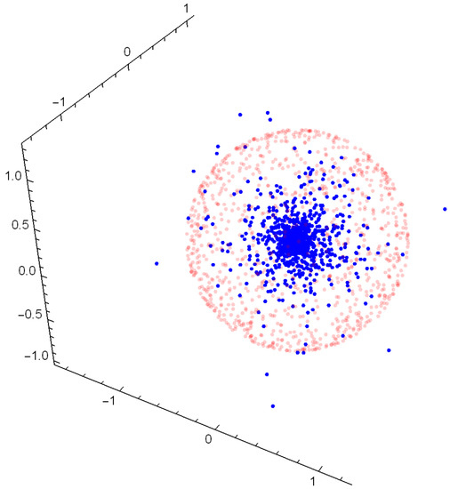
(Uniform-Gamma). Consider again Example 4, where R is a gamma random variable with $\vartheta =0.3$ and $\alpha =1$. In order to generate a random d-vector from a spherical uniform distribution on the unit ball, we first generate a d-variate standard normal random vector $\mathbf{Z}$ and define $\mathbf{U}=\mathbf{Z}/\left|\right|\mathbf{Z}\left|\right|$ and then use (3) to generate $\mathbf{W}$.

Figure 1, for $d=3$, reports 100 random values, respectively, for $\mathbf{U}$ (transparent red) and $\mathbf{W}$ (solid blue); note that the values of $\mathbf{W}$ are much more concentrated towards the center, with approximately 10% of the points going out of the unit sphere.

Figure 1. One hundred random values, respectively, for $\mathbf{U}$ (transparent red) and $\mathbf{W}$ (solid blue).

Numerical true and estimated values of the moments ${\mu }_{W,2m}$ and ${\nu }_m$ are computed by using Formulae (18) and (20). The tables below report population values and sample estimates for different sample sizes. As one can see, these values are in good agreement for all sample sizes but for very high-order moments, which require very large sample sizes to obtain reasonable approximations.

Consider now the case of multivariate moments and cumulants of $\mathbf{W}$ whose formulae are provided in Theorem 2. Set $d=3$. Since the result lies in univariate moments and cumulants, the application of the theorem reduces to computing the term $L_{m_2}^{-1}{vec}^{\otimes m}{\mathbf{I}}_d$ (see Section 5.1 for $L_{m_2}^{-1}$).

The second univariate cumulant of $\mathbf{W}$, viz. the variance, is given in Table 1 and $vec{\mathbf{I}}_3$ provides the correct form for ${\mathbf{\kappa }}_{\mathbf{W},2}^{\otimes }$.

Table 1. Moments ${\mu }_{W,2m}$ (see (18)). True and sample estimates.

2m	2	4	6	8	10
True	0.0600	0.0388	0.0750	0.2939	1.9480
Sample $n={10}^3$	0.0597	0.0331	0.0412	0.0718	0.1438
Sample $n={10}^4$	0.0597	0.0371	0.0606	0.1612	0.5439
Sample $n={10}^5$	0.0602	0.0394	0.0734	0.2401	1.0682
Sample $n={10}^6$	0.0601	0.0391	0.0740	0.2614	1.3682

Computations show that ${\kappa }_{W,4}=0.02808$ and the kurtosis ${\kappa }_{W,4}/{\kappa }_{W,2}^2=7.8$, which actually corresponds to $3{\kappa }_0$ given in Table 2. Note that for $d=3$, the fourth cumulant vector is of dimension $d^4=81$; in general, its elements are not all distinct, and the distinct elements can be recovered by linear transformations (see [30] for further discussion). The cumulant vector of the distinct elements, using the formula for ${\mathbf{L}}_{2_2}^{-1}$ given in Remark 1, reads

$$distinct-{\mathbf{L}}_{2_2}^{-1}{vec}^{\otimes 2}{\mathbf{I}}_3={\left(1,0,0,\frac{1}{3},0,\frac{1}{3},0,0,0,0,1,0,\frac{1}{3},0,1\right)}^{⊺}.$$

Direct estimation of the fourth cumulant vector from the simulated data confirms the theoretical results. The knowledge of ${\mathbf{\kappa }}_{\mathbf{W},4}^{\otimes }$ and Formulae (38) and (39) obtains ${\beta }_{2,d}=54$ (note also that ${\beta }_{2,d}=d(d+2)({\kappa }_0+1)$ and $VecB\left(\mathbf{Y}\right)={(13,0,0,0,13,0,0,0,13)}^{⊺}$).

Table 2. Moments ${\nu }_m$ (see (20)) and kurtosis parameter ${\kappa }_0$. True and sample estimates.

m	1	2	3	4	${\mathit{\kappa }}_0$
True	0.0300	0.00324	0.00062	0.00017	2.60
Sample $n={10}^3$	0.0334	0.00477	0.00132	0.00040	3.28
Sample $n={10}^4$	0.0313	0.00331	0.00052	0.00009	2.38
Sample $n={10}^5$	0.0303	0.00333	0.00067	0.00019	2.62

Example 6.

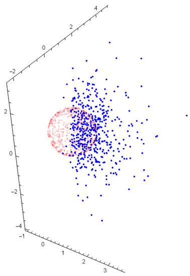
Set $d=3$ and let $\mathbf{X}$ be a trivariate $S{t}_3\left(\mathbf{0},\Omega ,\alpha ,p\right)$ random vector, with $p=15$, $\alpha ={(10,5,0)}^{⊺}$ and Ω be the identity matrix. Random numbers generated from the distribution of $\mathbf{X}$ and for comparison from a trivariate $\mathbf{U}$ are in Figure 2. From (32), we obtain that $\delta ={(0.89,0.45,0)}^{⊺}$ approximately.

Figure 2. Five hundred random values, respectively, for $\mathbf{U}$ (transparent red) and $\mathbf{X}$ (blue).

We run a Monte Carlo simulation where 1000 samples of size $n=1000$ are generated from the $S{t}_3$ distribution defined above. For each of the 1000 samples, measures of location, variance, skewness and kurtosis are computed applying Formulae (34) and (35) and the results of Lemmas 3 and 4. Empirical averages of the statistics are calculated, denoting the empirical expected value as error.

As far as mean and variance of $\mathbf{X}$, we compare the true and empirical expected values (values are rounded to the second decimal point).

$$E\mathbf{X}={(0.75,0.37,0)}^{⊺},\stackrel{\wedge }{E}\mathbf{X}={(0.75,0.37,\simeq 0)}^{⊺},$$

$$Var\mathbf{X}=\left(\begin{array}{ccc}0.59& -0.28& 0.\\ -0.28& 1.01& 0.\\ 0.& 0.& 1.15\end{array}\right),\stackrel{\wedge }{E}\left(Var\mathbf{X}\right)=\left(\begin{array}{ccc}0.59& -0.28& \simeq 0.\\ -0.28& 1.02& \simeq 0.\\ \simeq 0.& \simeq 0.& 1.15\end{array}\right).$$

As far as the skewness vector is concerned, let ${\kappa }_3={\kappa }_{Y,3}^{\otimes }$. Note that ${\kappa }_3$ has dimension $d^3$ and has $d(d+1)(d+2)/6$ distinct values; for $d=3$, these are 10. True and empirical expected values of the distinct values are (subscript D denotes distinct values)

$$\begin{array}{cc}\hfill {\kappa }_{3,D}& ={(0.94,0.38,0,0.26,0,0.09,0.22,0,0.05,0)}^{⊺},\hfill \\ \hfill \stackrel{\wedge }{E}\left({\kappa }_{3,D}\right)& ={(0.92,0.38,\simeq 0,0.26,\simeq 0,0.09,0.22,\simeq 0,0.05,\simeq 0)}^{⊺}.\hfill \end{array}$$

Using ${\kappa }_3$, from the results in Section 4.1, one gets ${\beta }_{1_d}=1.6$ and $s\left(\mathbf{Y}\right)={(1.29,0.64,0)}^{⊺}$. Considering now the kurtosis, define ${\kappa }_4={\kappa }_{Y,4}^{\otimes }$. There are $d(d+1)(d+2)(d+3)/24$ distinct values in ${\kappa }_4$, which has dimension $d^4$; for $d=3$, the distinct values are 15. True and empirical expected values of the distinct values are

$$\begin{array}{cc}\hfill {\kappa }_{4,D}& ={(1.61,0.50,0,0.44,0,0.20,0.15,0,0.01,0,0.63,0,0.19,0,0.55)}^{⊺},\hfill \\ \hfill \stackrel{\wedge }{E}\left({\kappa }_{4,D}\right)& ={(1.49,0.48,\simeq 0,0.42,\simeq 0,0.18,0.13,\simeq 0,\simeq 0,\simeq 0,0.60,\simeq 0,0.18,\simeq 0,0.52)}^{⊺}.\hfill \end{array}$$

Again, using ${\kappa }_4$, from the results in Section 4.1, one gets ${\beta }_{2,3}=19.45$ and $VecB\left(\mathbf{Y}\right)=$${(2.25,0.66,0,0.66,1.26,0,0,0,0.93)}^{⊺}$.

5. Proofs

Proof of Theorem 1.

Differentiate $g\left({\lambda }_j^2\right)$ to obtain the moments of $W_j$ in terms of generator moments,

$$\frac{\partial }{\partial {\lambda }_j}g\left({\lambda }_j^2\right)=g^{\left(1\right)}\left({\lambda }_j^2\right)\left(2{\lambda }_j\right),\frac{{\partial }^2}{\partial {\lambda }_j^2}g\left({\lambda }_j^2\right)=g^{\left(2\right)}\left({\lambda }_j^2\right){\left(2{\lambda }_j\right)}^2+2g^{\left(1\right)}\left({\lambda }_j^2\right).$$

(41)

Proceed by noting that the coefficients of $g^{\left(n\right)}\left({\lambda }_j^2\right)={\partial }^n/\partial {\lambda }_j^{n}g\left({\lambda }_j^2\right)$ are scalar valued series, say, $b_n^j$, when we take the derivatives of a compound function $g\left({\lambda }_j^2\right)$. Therefore, we have

$$g^{\left(n\right)}\left({\lambda }_j^2\right)=b_n^n{g}^{\left(n\right)}\left({\lambda }_j^2\right){\left(2{\lambda }_j\right)}^n+b_n^{n-1}{g}^{\left(n-1\right)}\left({\lambda }_j^2\right){\left(2{\lambda }_j\right)}^{\left(n-2\right)}+b_n^{n-m}{g}^{\left(n-m\right)}\left({\lambda }_j\right){\left(2{\lambda }_j\right)}^{\left(n-2m\right)},$$

(42)

where $m=\left[\frac{n}{2}\right]$, and the coefficients $b_n^k$ fulfill the following recursion

$$b_n^n=1\mathrm{and}{b}_n^{n-k}=2b_{n-1}^{n-k}\left(n-2k+1\right)+b_{n-1}^{n-k-1},k=1,\dots ,m=\left[\frac{n}{2}\right].$$

If n is odd then the power of the last term in (42) is $n-2\left[n/2\right]=1$, then $g^{\left(n\right)}\left(0\right)=0$; otherwise, $g^{\left(n\right)}\left(0\right)=b_n^{n/2}{g}^{\left(m\right)}\left(0\right)$; hence,

$$E{W}_j^n=\left\{\begin{array}{cccc}0& \mathrm{if}& n& \mathrm{odd},\\ {\left(-1\right)}^m{b}_{2m}^m{g}^{\left(m\right)}\left(0\right)& \mathrm{if}& n=2m& \mathrm{even}.\end{array}\right.$$

As has been noticed by [6], $b_n^k$ does not depend on g. Hence, we may choose, say, $g\left(t\right)=exp\left(-t^2\right)$ (being a valid characteristic function) and derive coefficients $b_{2m}^m$, resulting in $b_{2m}^m=2^m\left(2m-1\right)!!$. Hence, for $n=2m$, $E{W}_j^{2m}={\left(-1\right)}^m{2}^m\left(2m-1\right)!!g^{\left(m\right)}\left(0\right)$. Now, (10) follows by changing ${\left(-1\right)}^m{g}^{\left(m\right)}\left(0\right)$ to the generator moment

$$E{W}_j^{2m}=\frac{\left(2m\right)!}{m!}{\nu }_m.$$

(43)

Observe that the right-hand side does not depend on the index j, so that all marginals are distributed equally. Plugging the cumulant generator function f into (42), it is readily seen that the odd generator cumulants ${\zeta }_m$ are also zero. The even-order cumulant for each $W_j$ is

$${Cum}_{2m}\left(W_j\right)=2^m\left(2m-1\right)!!{\zeta }_m=\frac{\left(2m\right)!}{m!}{\zeta }_m.$$

Formula (17) utilizes Faà di Bruno’s Formula (9) connecting the generator cumulants ${\zeta }_m$ in terms of generator moments ${\nu }_m$. □

Proof of Corollary 1.

The general Formula (17) is based on the formula for the “cumulants” ${\zeta }_m$ in terms of “moments” ${\nu }_j$. Thus

$${\tilde{\kappa }}_m=\frac{{\zeta }_m}{{\nu }_1^m}=\sum _{r=1}^m{(-1)}^{r-1}(r-1)!\sum _{\Sigma {\ell }_j=r,\Sigma j{\ell }_j=m}\frac{m!}{{\prod }_{j=1}^{\ell }{\ell }_j!}\prod _{j=1}^{\ell }{\left(\frac{{\nu }_j}{j!{\nu }_1^j}\right)}^{{\ell }_j},$$

and we change the ratio ${\nu }_j/{\nu }_1^j={\tilde{\mu }}_2+1$, so that the assertion (17) follows. □

Proof of Theorem 2.

The key point in the proof is understanding the form of the derivative $D_{\lambda }^{\otimes 2m}{\left({\lambda }^{⊺}\lambda \right)}^m$. First, we notice that

$$D_{\lambda }^{\otimes 2m}{\left({\lambda }^{⊺}\lambda \right)}^m=D_{\lambda }^{\otimes 2m}{\prod }_{j=1}^{{}^m}{f}_j\left(\lambda \right),$$

where $f_j\left(\lambda \right)={\lambda }^{⊺}\lambda$; that is, we can use the general Leibnitz rule, and symmetrize by ${\mathbf{S}}_{d{\mathbf{1}}_{2m}}$,

$$\begin{array}{ccc}& D_{\lambda }^{\otimes 2m}{\prod }_j{f}_j\left(\lambda \right)& =\sum _{\Sigma k_{1:m}=2m}\left(\genfrac{}{}{0pt}{}{2m}{k_{1:m}}\right){\prod }_j^{\otimes }{D}_{\lambda }^{\otimes k_j}{f}_j\left(\lambda \right),\hfill \\ & & \stackrel{Ⓢ}{=}\left(2m\right)!{vec}^{\otimes m}{\mathbf{I}}_d,\hfill \end{array}$$

(44)

since the only nonzero term is when $k_j=2$, $j=1:m$, then $D_{\lambda }^{\otimes 2}{f}_j\left(\lambda \right)=2vec{\mathbf{I}}_d$. Therefore, we have

$$\left(\genfrac{}{}{0pt}{}{2m}{2_{{\mathbf{1}}_m}}\right)2^m=\frac{\left(2m\right)!}{{\left(2!\right)}^m}{2}^m=\left(2m\right)!,$$

terms in the sum (44), each equals ${vec}^{\otimes m}{\mathbf{I}}_d$, hence the assertion follows. □

Proof of Lemma 3.

Direct calculation shows

$$\begin{array}{ccc}\hfill {\mathbf{\kappa }}_{\mathbf{X},3}^{\otimes }& \stackrel{Ⓢ}{=}& {\underline{Cum}}_1\left({\mathbf{\kappa }}_{\mathbf{X},3|R_p}^{\otimes }\right)+3{\underline{Cum}}_2\left({\mathbf{\kappa }}_{\mathbf{X},1|R_p}^{\otimes },{\mathbf{\kappa }}_{\mathbf{X},2|R_p}^{\otimes }\right)+{\underline{Cum}}_3\left({\mathbf{\kappa }}_{\mathbf{X},1|R_p}^{\otimes }\right)\hfill \\ & =& {\underline{Cum}}_1\left(R_p^3{\mathbf{\kappa }}_{\mathbf{V},3}^{\otimes }\right)+3{\underline{Cum}}_2\left(R_p{\mathbf{\kappa }}_{\mathbf{V},1}^{\otimes },R_p^2{\mathbf{\kappa }}_{\mathbf{V},2}^{\otimes }\right)+{\underline{Cum}}_3\left(R_p{\mathbf{\kappa }}_{\mathbf{V},1}^{\otimes }\right)\hfill \\ & =& {\kappa }_{R_p^3,1}{\mathbf{\kappa }}_{\mathbf{V},3}^{\otimes }+3{\kappa }_{R_p,R_p^2}\left({\mathbf{\kappa }}_{\mathbf{V},1}^{\otimes }\otimes {\mathbf{\kappa }}_{\mathbf{V},2}^{\otimes }\right)+{\kappa }_{R_p,3}{\mathbf{\kappa }}_{\mathbf{V},1}^{\otimes 3}\hfill \\ & =& {\kappa }_{R_p^3,1}{\kappa }_{\left|Z\right|,3}{\delta }^{\otimes 3}+3{\kappa }_{R_p,R_p^2}{\kappa }_{\left|Z\right|,1}\left(\delta \otimes \left(vec\Omega -{\kappa }_{\left|Z\right|,2}^{☆}{\delta }^{\otimes 2}\right)\right)+{\kappa }_{R_p,3}{\kappa }_{\left|Z\right|,1}^3{\delta }^{\otimes \mathbf{3}}\hfill \\ & =& \left({\kappa }_{R_p^3,1}{\kappa }_{\left|Z\right|,3}+3{\kappa }_{R_p,R_p^2}{\kappa }_{\left|Z\right|,1}{\kappa }_{\left|Z\right|,2}^{☆}+{\kappa }_{R_p,3}{\kappa }_{\left|Z\right|,1}^3\right){\delta }^{\otimes 3}+3{\kappa }_{R_p,R_p^2}{\kappa }_{\left|Z\right|,1}\delta \otimes vec\Omega \hfill \end{array}$$

where ${\kappa }_{\left|Z\right|,2}^{★}=-2/\pi$, the coefficients of ${\mathbf{\kappa }}_{\mathbf{X},3}^{\otimes }$ in the expression are given in (36). We obtain (${\kappa }_{R_p^3,1}={\mu }_{R_p,3}$)

$${\mathbf{\kappa }}_{\mathbf{X},3}^{\otimes }\stackrel{Ⓢ}{=}\left({\mu }_{R_p,3}{\kappa }_{\left|Z\right|,3}+{\kappa }_{R_p,3}{\kappa }_{\left|Z\right|,1}^3\right){\delta }^{\otimes 3}+3{\kappa }_{R_p,R_p^2}{\kappa }_{\left|Z\right|,1}\left(vec\Omega -\frac{2}{\pi }{\delta }^{\otimes 2}\right).$$

The quantities in the coefficient of ${\delta }^{\otimes 3}$ are given in (33), leading to the result of the lemma. □

Proof of Lemma 4.

Writing $G_{-1}=G_{-1}\left(p\right)$, one can derive the formula

$${\mathbf{\kappa }}_{\mathbf{X},4}\stackrel{Ⓢ}{=}{\kappa }_{R_p^4,1}{\mathbf{\kappa }}_{\mathbf{V},4}^{\otimes }+4{\kappa }_{R_p,R_p^3}\left({\mathbf{\kappa }}_{\mathbf{V},1}^{\otimes }\otimes {\mathbf{\kappa }}_{\mathbf{V},3}^{\otimes }\right)+3{\kappa }_{R_p^2,R_p^2}{\mathbf{\kappa }}_{\mathbf{V},2}^{\otimes 2}+6{\kappa }_{R_p,R_p,R_p^2}{\mathbf{\kappa }}_{\mathbf{V},1}^{\otimes 2}\otimes {\mathbf{\kappa }}_{\mathbf{V},2}^{\otimes }+{\kappa }_{R_p,4}{\delta }^{\otimes 4}$$

from (36) for ${\mathbf{\kappa }}_{\mathbf{X},4}$ directly. We pay particular attention to the value of ${\mathbf{\kappa }}_{\mathbf{V},2}^{\otimes }$

$$\begin{array}{ccc}& & {\mathbf{\kappa }}_{\mathbf{X},4}\stackrel{Ⓢ}{=}\left({\kappa }_{R_p^4,1}{\kappa }_{\left|Z\right|,4}+4{\kappa }_{R_p,R_p^3}{\kappa }_{\left|Z\right|,1}{\kappa }_{\left|Z\right|,3}+{\kappa }_{R_p,4}{\kappa }_{\left|Z\right|,1}^4\right){\delta }^{\otimes 4}\hfill \\ & & +3{\kappa }_{R_p^2,2}{\left(vec\Omega -\frac{2}{\pi }{\delta }^{\otimes 2}\right)}^{\otimes 2}+6{\kappa }_{R_p,R_p,R_p^2}{\kappa }_{\left|Z\right|,1}^2\left(vec\Omega -\frac{2}{\pi }{\delta }^{\otimes 2}\right)\otimes {\delta }^{\otimes 2}\hfill \end{array}$$

we have ${\kappa }_{R_p^4,1}={\mu }_{R_p,4}$; moreover,

$$\begin{array}{ccc}& & {\mathbf{\kappa }}_{\mathbf{X},4}\stackrel{Ⓢ}{=}\left({\kappa }_{R_p^4,1}{\kappa }_{\left|Z\right|,4}+4{\kappa }_{R_p,R_p^3}{\kappa }_{\left|Z\right|,1}{\kappa }_{\left|Z\right|,3}+{\kappa }_{R_p,4}{\kappa }_{\left|Z\right|,1}^4+3{\left(\frac{2}{\pi }\right)}^2{\kappa }_{R_p^2,2}-6{\left(\frac{2}{\pi }\right)}^2{\kappa }_{R_p,R_p,R_p^2}\right)\hfill \\ & & \times {\delta }^{\otimes 4}+3{\kappa }_{R_p^2,2}{\left(vec\Omega \right)}^{\otimes 2}+6\frac{2}{\pi }\left({\kappa }_{R_p,R_p,R_p^2}-{\kappa }_{R_p^2,2}\right)vec\Omega \otimes {\delta }^{\otimes 2}\hfill \end{array}$$

and

$${\kappa }_{R_p^2,2}=\frac{2p^2}{\left(p-4\right){\left(p-2\right)}^2},$$

$${\kappa }_{R_p,R_p,R_p^2}-{\kappa }_{R_p^2,2}=-{\left(\frac{p}{2}\right)}^2{G}_{-1}^2\frac{4}{\left(p-2\right)\left(p-3\right)}.$$

The coefficient of ${\delta }^{\otimes 4}$ follows

$$\begin{array}{ccc}& & {\mu }_{R_p,4}{\kappa }_{\left|Z\right|,4}+4{\kappa }_{R_p,R_p^3}{\kappa }_{\left|Z\right|,1}{\kappa }_{\left|Z\right|,3}+3{\left(\frac{2}{\pi }\right)}^2{\kappa }_{R_p^2,2}-6{\left(\frac{2}{\pi }\right)}^2{\kappa }_{R_p,R_p,R_p^2}+{\kappa }_{R_p,4}{\kappa }_{\left|Z\right|,1}^4\hfill \\ & =& \left(-6{\left(\frac{2}{\pi }\right)}^2+4\frac{2}{\pi }\right){\mu }_{R_p,4}+\left(8{\left(\frac{2}{\pi }\right)}^2-4\frac{2}{\pi }\right){\kappa }_{R_p,R_p^3}+3{\left(\frac{2}{\pi }\right)}^2{\kappa }_{R_p^2,2}\hfill \\ & & -6{\left(\frac{2}{\pi }\right)}^2{\kappa }_{R_p,R_p,R_p^2}+{\kappa }_{R_p,4}{\left(\frac{2}{\pi }\right)}^2\hfill \\ & =& {\left(\frac{2}{\pi }\right)}^2\left(-6{\mu }_{R_p,4}+8{\kappa }_{R_p,R_p^3}+3{\kappa }_{R_p^2,2}-6{\kappa }_{R_p,R_p,R_p^2}+{\kappa }_{R_p,4}\right)+4\frac{2}{\pi }\left({\mu }_{R_p,4}-{\kappa }_{R_p,R_p^3}\right)\hfill \end{array}$$

where $-6{\mu }_{R_p,4}+8{\kappa }_{R_p,R_p^3}+3{\kappa }_{R_p^2,2}-6{\kappa }_{R_p,R_p,R_p^2}+{\kappa }_{R_p,4}=-3p^2{G}_{-1}^4/2,$ and ${\mu }_{R_p,4}-{\kappa }_{R_p,R_p^3}=p^2{G}_{-1}^2/2(p-3).$ □

Proof of Theorem 3.

We use (23) and obtain

$${\mathbf{\kappa }}_{\mathbf{X},n}^{\otimes }={\mathbf{S}}_{d{\mathbf{1}}_n}\sum _{r=1}^n\sum _{\begin{array}{c}\Sigma {\ell }_j=r,\\ \Sigma j{\ell }_j=n\end{array}}\frac{n!}{{\prod }_{j=1}^n{\ell }_j!{\left(j!\right)}^{{\ell }_j}}{\underline{Cum}}_r\left({\left({\mathbf{\kappa }}_{\mathbf{X},1|R_p}^{\otimes }\right)}_{1:{\ell }_1},\dots ,{\left({\mathbf{\kappa }}_{\mathbf{X},n|R_p}^{\otimes }\right)}_{1:{\ell }_n}\right)$$

where ${\mathbf{\kappa }}_{\mathbf{X},j|R_p}^{\otimes }={\underline{Cum}}_j{\left(\mathbf{X}|R_p\right)}_{1:{\ell }_j}$ denotes ${\ell }_j$ copies of ${\mathbf{\kappa }}_{\mathbf{X},j|R_p}^{\otimes }$, as usual, including the case ${\ell }_j=0$, when ${\underline{Cum}}_j\left(\mathbf{X}|R_p\right)$ is missing from ${\underline{Cum}}_r$. Therefore, ${\underline{Cum}}_r$ contains exactly r variables. The conditional cumulant

$${\mathbf{\kappa }}_{\mathbf{X},j|R_p}^{\otimes }={\mathbf{\kappa }}_{R_p\mathbf{V},j|R_p}^{\otimes }=R_p^j{\mathbf{\kappa }}_{\mathbf{V},j}^{\otimes },$$

since $R_p$ and $\mathbf{X}$ are independent. We apply Lemma 4 of [29], obtaining the ${\mathbf{\kappa }}_{\mathbf{V},j}^{\otimes }$, and get

$$\begin{array}{ccc}\hfill {\mathbf{\kappa }}_{\mathbf{X},n}^{\otimes }& =& n!\sum _{r=1}^n\sum _{\begin{array}{c}\Sigma {\ell }_j=r,\\ \Sigma j{\ell }_j=n\end{array}}\frac{{\mathcal{C}}_r\left(R_p,{\ell }_{1:n}\right)}{{\prod }_{j=1}^n{\ell }_j!{\left(j!\right)}^{{\ell }_j}}{\prod }_{j=1:n}^{\otimes }{\mathbf{\kappa }}_{\mathbf{V},j}^{\otimes {\ell }_j}\hfill \\ & =& n!{\mathbf{S}}_{d{\mathbf{1}}_n}\sum _{r=1}^n\sum _{\begin{array}{c}\Sigma {\ell }_j=r,\\ \Sigma j{\ell }_j=n\end{array}}{\mathcal{C}}_r\left(R_p,{\ell }_{1:n}\right)\prod _{j=1,j\ne 2}^n\frac{1}{{\ell }_j!}{\left(\frac{{\kappa }_{\left|Z\right|,j}}{j!}\right)}^{{\ell }_j}\frac{1}{{\ell }_2!}{\left(\frac{1}{2!}\right)}^{{\ell }_2}{\mathbf{\kappa }}_{\mathbf{V},2}^{\otimes {\ell }_2}\otimes {\delta }^{\otimes \left(n-2{\ell }_2\right)},\hfill \end{array}$$

where we have separated $j=2$, since the second-order cumulant ${\mathbf{\kappa }}_{\mathbf{V},2}^{\otimes }$ is different in the product. □

5.1. Commutator and Symmetrizer Matrices

Commutator matrices ${\mathbf{K}}_{\mathfrak{p}}$ change the order of the tensor products of vectors according to permutation $\mathfrak{p}$; see [29] for more details. Commutator matrix $\mathbf{L}$ corresponds to type $\ell ={\ell }_{1:n}$, such that nonzero ${\ell }_j$s of ℓ define the sum of commutator matrices as follows

$${\mathbf{L}}_{l_{r:1}}^{-1}=\sum _{{\mathcal{K}}_{\left\{r|\ell \right\}}\in {\mathcal{P}}_n}{\mathbf{K}}_{\mathfrak{p}\left({\mathcal{K}}_{\left\{r|\ell \right\}}\right).}^{-1}$$

where index $l_{r:1}$ is defined by the following way: if ${\ell }_j\ne 0$ then set ${\ell }_j$ by $l_j$, where $l$ denotes the actual value of ${\ell }_j$; for instance, if ${\ell }_j=3$, then $l_j=3_j$. The summation is taken over all partition ${\mathcal{K}}_{\left\{r|\ell \right\}}$ of the set 1:n, having type ℓ and size r.

Ref. [49] uses the symmetrizer matrix ${\mathbf{S}}_{d{\mathbf{1}}_q}$ for symmetrization of a T-product of q vectors with the same dimension d; that is, the result of ${\mathbf{S}}_{d{\mathbf{1}}_4}\left({\underline{a}}_1\otimes {\underline{a}}_2\otimes {\underline{a}}_3\otimes {\underline{a}}_4\right)$ is a vector of dimension $d^4$, and symmetric in ${\underline{a}}_j$. It can be computed as

$${\mathbf{S}}_{d{\mathbf{1}}_q}=\frac{1}{q!}\sum _{p\in P_q}{\mathbf{K}}_p,$$

(45)

where $P_q$ denotes the set of all permutations of the numbers 1:q; the sum includes $q!$ terms. The symmetrizer ${\mathbf{S}}_{d{\mathbf{1}}_q}$ provides an orthogonal projection to the subspace of ${\mathbb{R}}^{d^q}$, which is invariant under the transformation ${\mathbf{S}}_{d{\mathbf{1}}_q}$. A vector will be called symmetrical if it belongs to that subspace.

References

- Kollo, T.; von Rosen, D. Advanced Multivariate Statistics with Matrices; Springer Science & Business Media: Berlin/Heidelberg, Germany, 2006; Volume 579. [Google Scholar]
- McCullagh, P. Tensor Methods in Statistics; Courier Dover Publications: New York, NY, USA, 2018. [Google Scholar]
- Ould-Baba, H.; Robin, V.; Antoni, J. Concise formulae for the cumulant matrices of a random vector. Linear Algebra Appl. 2015, 485, 392–416. [Google Scholar] [CrossRef]
- Kolda, T.G.; Bader, B.W. Tensor decompositions and applications. SIAM Rev. 2009, 51, 455–500. [Google Scholar] [CrossRef]
- Qi, L. Rank and eigenvalues of a supersymmetric tensor, the multivariate homogeneous polynomial and the algebraic hypersurface it defines. J. Symb. Comput. 2006, 41, 1309–1327. [Google Scholar] [CrossRef]
- Berkane, M.; Bentler, P.M. Moments of elliptically distributed random variates. Stat. Probab. Lett. 1986, 4, 333–335. [Google Scholar] [CrossRef]
- Mardia, K.V. Measures of Multivariate Skewness and Kurtosis with Applications. Biometrika 1970, 57, 519–530. [Google Scholar] [CrossRef]
- Malkovich, J.F.; Afifi, A.A. On tests for multivariate normality. J. Am. Stat. Assoc. 1973, 68, 176–179. [Google Scholar] [CrossRef]
- Srivastava, M.S. A measure of skewness and kurtosis and a graphical method for assessing multivariate normality. Stat. Probab. Lett. 1984, 2, 263–267. [Google Scholar] [CrossRef]
- Koziol, J.A. A Note on Measures of Multivariate Kurtosis. Biom. J. 1989, 31, 619–624. [Google Scholar] [CrossRef]
- Móri, T.F.; Rohatgi, V.K.; Székely, G.J. On multivariate skewness and kurtosis. Theory Probab. Appl. 1994, 38, 547–551. [Google Scholar] [CrossRef]
- Shoukat Choudhury, M.; Shah, S.; Thornhill, N. Diagnosis of poor control-loop performance using higher-order statistics. Automatica 2004, 40, 1719–1728. [Google Scholar] [CrossRef]
- Oja, H.; Sirkiä, S.; Eriksson, J. Scatter matrices and independent component analysis. Austrian J. Stat. 2006, 35, 175–189. [Google Scholar]
- Balakrishnan, N.; Brito, M.R.; Quiroz, A.J. A vectorial notion of skewness and its use in testing for multivariate symmetry. Commun. Stat. Theory Methods 2007, 36, 1757–1767. [Google Scholar] [CrossRef]
- Kollo, T. Multivariate skewness and kurtosis measures with an application in ICA. J. Multivar. Anal. 2008, 99, 2328–2338. [Google Scholar] [CrossRef]
- Tyler, D.E.; Critchley, F.; Dümbgen, L.; Oja, H. Invariant co-ordinate selection. J. R. Stat. Soc. Ser. B (Stat. Methodol.) 2009, 71, 549–592. [Google Scholar] [CrossRef]
- Ilmonen, P.; Nevalainen, J.; Oja, H. Characteristics of multivariate distributions and the invariant coordinate system. Stat. Probab. Lett. 2010, 80, 1844–1853. [Google Scholar] [CrossRef]
- Peña, D.; Prieto, F.J.; Viladomat, J. Eigenvectors of a kurtosis matrix as interesting directions to reveal cluster structure. J. Multivar. Anal. 2010, 101, 1995–2007. [Google Scholar] [CrossRef]
- Tanaka, K.; Yamada, T.; Watanabe, T. Applications of Gram–Charlier expansion and bond moments for pricing of interest rates and credit risk. Quant. Financ. 2010, 10, 645–662. [Google Scholar] [CrossRef]
- Huang, H.H.; Lin, S.H.; Wang, C.P.; Chiu, C.Y. Adjusting MV-efficient portfolio frontier bias for skewed and non-mesokurtic returns. N. Am. J. Econ. Financ. 2014, 29, 59–83. [Google Scholar] [CrossRef]
- Wang, Y.; Fan, J.; Yao, Y. Online monitoring of multivariate processes using higher-order cumulants analysis. Ind. Eng. Chem. Res. 2014, 53, 4328–4338. [Google Scholar] [CrossRef]
- Lin, S.H.; Huang, H.H.; Li, S.H. Option pricing under truncated Gram–Charlier expansion. N. Am. J. Econ. Financ. 2015, 32, 77–97. [Google Scholar] [CrossRef]
- Loperfido, N. Singular value decomposition of the third multivariate moment. Linear Algebra Appl. 2015, 473, 202–216. [Google Scholar] [CrossRef]
- De Luca, G.; Loperfido, N. Modelling multivariate skewness in financial returns: A SGARCH approach. Eur. J. Financ. 2015, 21, 1113–1131. [Google Scholar] [CrossRef]
- Fiorentini, G.; Planas, C.; Rossi, A. Skewness and kurtosis of multivariate Markov-switching processes. Comput. Stat. Data Anal. 2016, 100, 153–159. [Google Scholar] [CrossRef]
- León, A.; Moreno, M. One-sided performance measures under Gram-Charlier distributions. J. Bank. Financ. 2017, 74, 38–50. [Google Scholar] [CrossRef]
- Nordhausen, K.; Oja, H.; Tyler, D.E.; Virta, J. Asymptotic and bootstrap tests for the dimension of the non-Gaussian subspace. IEEE Signal Process. Lett. 2017, 24, 887–891. [Google Scholar] [CrossRef]
- Loperfido, N. Skewness-based projection pursuit: A computational approach. Comput. Stat. Data Anal. 2018, 120, 42–57. [Google Scholar] [CrossRef]
- Jammalamadaka, S.; Taufer, E.; Terdik, G.H. On Multivariate Skewness and Kurtosis. Sankhya A 2021, 83-A, 607–644. [Google Scholar] [CrossRef]
- Jammalamadaka, S.; Taufer, E.; Terdik, G.H. Asymptotic theory for statistics based on cumulant vectors with applications. Scand. J. Stat. 2021, 48, 708–728. [Google Scholar] [CrossRef]
- Azzalini, A.; Capitanio, A. Distributions generated by perturbation of symmetry with emphasis on a multivariate skew t-distribution. J. R. Stat. Soc. Ser. B (Stat. Methodol.) 2003, 65, 367–389. [Google Scholar] [CrossRef]
- Azzalini, A.; Regoli, G. Some properties of skew-symmetric distributions. Ann. Inst. Stat. Math. 2011, 64, 857–879. [Google Scholar] [CrossRef]
- Sahu, S.K.; Dey, D.K.; Branco, M.D. A new class of multivariate skew distributions with applications to Bayesian regression models. Can. J. Stat. 2003, 31, 129–150. [Google Scholar] [CrossRef]
- Jones, M.C.; Faddy, M. A skew extension of the t-distribution, with applications. J. R. Stat. Soc. Ser. B (Stat. Methodol.) 2003, 65, 159–174. [Google Scholar] [CrossRef]
- Adcock, C.; Azzalini, A. A Selective Overview of Skew-Elliptical and Related Distributions and of Their Applications. Symmetry 2020, 12, 118. [Google Scholar] [CrossRef]
- Rao Jammalamadaka, S.; Subba Rao, T.; Terdik, G. Higher Order Cumulants of Random Vectors and Applications to Statistical Inference and Time Series. Sankhya Ser. A Methodol. 2006, 68, 326–356. [Google Scholar]
- NIST Digital Library of Mathematical Functions. Release 1.0.17 of 2017-12-22. 2020. Available online: http://dlmf.nist.gov/ (accessed on 23 June 2021).
- Fang, K.W.; Kotz, S.; Ng, K.W. Symmetric Multivariate and Related Distributions; Chapman and Hall: London, UK; CRC: Boca Raton, FL, USA, 2017. [Google Scholar]
- Muirhead, R.J. Aspects of Multivariate Statistical Theory; John Wiley & Sons: Hoboken, NJ, USA, 2009; Volume 197. [Google Scholar]
- Anderson, T.W. An Introduction to Multivariate Statistical Analysis; John Wiley & Sons: Hoboken, NJ, USA, 2003. [Google Scholar]
- Steyn, H. On the problem of more than one kurtosis parameter in multivariate analysis. J. Multivar. Anal. 1993, 44, 1–22. [Google Scholar] [CrossRef][Green Version]
- Azzalini, A.; Dalla Valle, A. The Multivariate Skew-Normal Distribution. Biometrika 1996, 83, 715–726. [Google Scholar] [CrossRef]
- Azzalini, A.; Capitanio, A. Statistical applications of the multivariate skew normal distribution. J. R. Stat. Soc. Ser. B (Stat. Methodol.) 1999, 61, 579–602. [Google Scholar] [CrossRef]
- Genton, M.G.; He, L.; Liu, X. Moments of skew-normal random vectors and their quadratic forms. Stat. Probab. Lett. 2001, 51, 319–325. [Google Scholar] [CrossRef]
- Azzalini, A. The Skew-normal Distribution and Related Multivariate Families. Scand. J. Stat. 2005, 32, 159–188. [Google Scholar] [CrossRef]
- Branco, M.D.; Dey, D.K. A General Class of Multivariate Skew-Elliptical Distributions. J. Multivar. Anal. 2001, 79, 99–113. [Google Scholar] [CrossRef]
- Kim, H.J.; Mallick, B.K. Moments of random vectors with skew t distribution and their quadratic forms. Stat. Probab. Lett. 2003, 63, 417–423. [Google Scholar] [CrossRef]
- Sutradhar, B.C. On the characteristic function of multivariate Student t-distribution. Can. J. Stat. 1986, 14, 329–337. [Google Scholar] [CrossRef]
- Holmquist, B. The D-Variate Vector Hermite Polynomial of Order. Linear Algebra Appl. 1996, 237/238, 155–190. [Google Scholar] [CrossRef]
Publisher’s Note: MDPI stays neutral with regard to jurisdictional claims in published maps and institutional affiliations. |
© 2021 by the authors. Licensee MDPI, Basel, Switzerland. This article is an open access article distributed under the terms and conditions of the Creative Commons Attribution (CC BY) license (https://creativecommons.org/licenses/by/4.0/).