A Compound Class of the Inverse Gamma and Power Series Distributions

Abstract

In this paper, the inverse gamma power series (IGPS) class of distributions asymmetric is introduced. This family is obtained by compounding inverse gamma and power series distributions. We present the density, survival and hazard functions, moments and the order statistics of the IGPS. Estimation is first discussed by means of the quantile method. Then, an EM algorithm is implemented to compute the maximum likelihood estimates of the parameters. Moreover, a simulation study is carried out to examine the effectiveness of these estimates. Finally, the performance of the new class is analyzed by means of two asymmetric real data sets.

1. Introduction

In the last few decades, several papers have discussed the derivation of new probabilistic families by compounding different distributions with the power series (PS) model. For example, the exponential geometric (EG, Adamidis and Loukas [1]), exponential Poisson (EP, Kus [2]) and exponential logarithmic (EL, Tahmasbi and Rezaei [3]) distributions. The exponential PS is introduced in Chahkandi and Ganjali [4], Morais and Barreto-Souza [5] presented the Weibull PS (WPS) class of distributions, Mahmoudi and Jafari [6] defined the generalized exponential PS (GEPS) distributions, Silva et al. [7], the extended Weibull PS (EWPS) and Bagheri et al. [8], the generalized modified Weibull PS distribution (GMWPS). More recently, Warahena-Liyanage and Pararai [9] introduce the Lindley PS distributions (LPS), Alizadeh et al. [10] study the exponentiated power Lindley PS class of distributions, Elbatal et al. [11] propose and study a new family of exponential Pareto PS and finally the Generalized Burr XII PS distribution was given by Elbatal et al. [12].

In this work, we propose to study the resulting model obtained by compounding the inverse gamma (IG) and the PS distribution introduced by Noack [13].

We say that a random variable X follows an IG distribution with shape parameter $\alpha >0$ and scale parameter $\beta >0$ (henceforward, the notation $X\sim IG(\alpha ,\beta )$ will be used) if its probability density function (pdf) is given by

$$\begin{array}{c}\hfill f(x;\alpha ,\beta )=\frac{{\beta }^{\alpha }}{\mathrm{\Gamma }\left(\alpha \right)}{x}^{-(\alpha +1)}{e}^{-\left(\frac{\beta }{x}\right)},x>0.\end{array}$$

(1)

and its survival function is

$$\begin{array}{c}\hfill S(x;\alpha ,\beta )=1-G\left(\frac{\beta }{x};\alpha \right),x>0,\end{array}$$

where $G(x;a)=\mathrm{\Gamma }(a,x)/\mathrm{\Gamma }\left(a\right)$ represents the survival function for the gamma distribution with shape parameter a and scale 1 and $\mathrm{\Gamma }(a,b)={\int }_b^{\infty }{u}^{a-1}{e}^{-u}du$ is the upper incomplete gamma function. Please note that $\mathrm{\Gamma }\left(a\right)=\mathrm{\Gamma }(a,0)$. The rth non-central moment for this distribution is given by $E\left(X^r\right)={\beta }^r(\alpha -r-1)!/(\alpha -1)!$, in particular for $\alpha >1$ we have $E\left(X\right)=\beta /(\alpha -1)$, and so for $\alpha >2$, $Var\left(X\right)={\beta }^2/{(\alpha -1)}^2(\alpha -2)$.

The remainder of the work is organized as follows. In Section 2, the Inverse Gamma PS (IGPS) probabilistic family is introduced and some properties including the density, survival and hazard functions, moments and statistical ordering are examined. Furthermore, some particular cases of this family are analyzed. Parameter estimation is discussed in Section 3, where quantile-matching estimation method and Expectation-Maximization (EM) algorithm are considered. In Section 4, a simulation analysis is carried out to test the performance of the estimates. Then, this family is applied to two real data sets. Section 5 concludes the paper.

2. The Model

Let $M\ge 1$ be the number of concurrent causes producing the event of interest in a subject. For instance, in a cancer context, M represents the number of carcinogenic cells that a patient has and, as a result of this number, it might trigger the metastasis process. In electronic circuits connected in series, M represents the number of components that the circuit has, so if one of those components fails, the entire circuit will fail. In credit scoring, M represents the number of different factors for which a customer stops paying their bills (economic, psychological, family, etc.). Let us also assume that M follows a PS distribution (Noack [13]) with probability mass function (pmf) given by

$$\begin{array}{c}\hfill P(M=m;\theta )=\frac{a_m{\theta }^m}{A\left(\theta \right)},m=1,2,\dots \end{array}$$

(2)

where $a_m>0$, $\theta >0$ is called the power parameter and the series function $A\left(\theta \right)={\sum }_{m=1}^{\infty }{a}_m{\theta }^m$. We highlight that the pmf in Equation (2) also corresponds to the generalized Power distribution discussed in Patil [14]. However, many works that have discussed this distribution referred to this model as PS model (see for instance, Adamidis and Loukas [1]; Morais and Barreto-Souza [5]). Hereafter, (2) will be denoted as PS$(\theta ,A(\theta \left)\right)$. In Table 1, for four members of the PS family, the values of $a_m$, $A\left(\theta \right)$ and parameter space $\mathrm{\Theta }$ are illustrated.

Table 1. Special cases of the PS$(\theta ,A(\theta \left)\right)$ distribution. For Binomial distribution q is considered known.

Distribution	Notation	${\mathit{a}}_{\mathit{m}}$	$\mathit{A}\left(\mathit{\theta }\right)$	$\mathbf{\Theta }$
Binomial	Bin($q,\theta )$	$\left(\genfrac{}{}{0pt}{}{q}{m}\right)$	${(1+\theta )}^q-1$	$(0,\infty )$
Poisson	Po($\theta$)	${(m!)}^{-1}$	$e^{\theta }-1$	$(0,\infty )$
Geometric	Geo($\theta$)	1	$\theta {(1-\theta )}^{-1}$	$(0,1)$
Logarithmic	Lo($\theta$)	${\left(m\right)}^{-1}$	$-log(1-\theta )$	$(0,1)$

Let the random variable $W_a$ denote the time when the ath concurrent causes produce the event of interest. $W_a$, $a=1,2,\dots ,M$, are assumed conditionally independent and identically distributed given M with common distribution IG$(\alpha ,\beta )$. The inverse gamma PS (henceforth, IGPS) model is defined as the marginal distribution of $T_{\left(1\right)}=min(W_1,\dots ,W_M)$. The survival function for the IGPS model is given by

$$S(t;\theta ,\alpha ,\beta )=\frac{A\left(\theta \left(1-G\left(\frac{\beta }{t};\alpha \right)\right)\right)}{A\left(\theta \right)}$$

(3)

and its corresponding density function is provided by

$$f(t;\theta ,\alpha ,\beta )=\frac{\theta {\beta }^{\alpha }}{\mathrm{\Gamma }\left(\alpha \right)}{t}^{-(\alpha +1)}{e}^{-\left(\frac{\beta }{t}\right)}\frac{A^{\prime }\left(\theta \left(1-G\left(\frac{\beta }{t};\alpha \right)\right)\right)}{A\left(\theta \right)}.$$

(4)

The hazard function is

$$h(t;\theta ,\alpha ,\beta )=\frac{\theta {\beta }^{\alpha }}{\mathrm{\Gamma }\left(\alpha \right)}{t}^{-(\alpha +1)}{e}^{-\left(\frac{\beta }{t}\right)}\frac{A^{\prime }\left(\theta \left(1-G\left(\frac{\beta }{t};\alpha \right)\right)\right)}{A\left(\theta \left(1-G\left(\frac{\beta }{t};\alpha \right)\right)\right)}.$$

(5)

Figure 1 shows the density and hazard functions for the inverse gamma Poisson (IGP), inverse gamma logarithmic (IGL), inverse gamma geometric (IGG) and inverse gamma binomial (IGB) distributions, respectively.

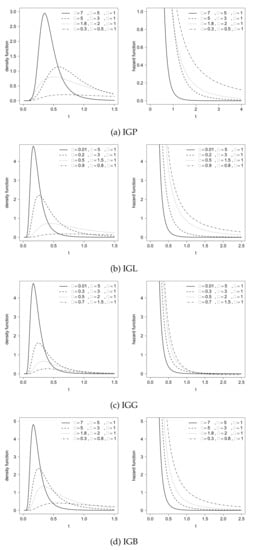
Figure 1. Density and hazard functions for the IGP, IGL, IGG and IGB distributions with different combinations for parameters.

In the following, we will examine some properties of the probability density function (4).

Proposition 1.

The IG distribution for $T_{\left(1\right)}$ is a limiting special case of the IGPS model when $\theta \to 0^{+}$.

Proof. 

We have that the cumulative distribution function (cdf) of the IG distribution for $T_{\left(1\right)}$ is given by $F\left(t\right)=F_{T_{\left(1\right)}}\left(t\right)=1-{\left(1-G\left(\frac{\beta }{t};\alpha \right)\right)}^c$, where $c=min\{m\in \mathbb{N}:a_m>0\}$. Therefore,

$$\underset{\theta \to 0^{+}}{lim}F(t;\theta ,\alpha ,\beta )=1-\underset{\theta \to 0^{+}}{lim}\frac{A\left(\theta \left(1-G\left(\frac{\beta }{t};\alpha \right)\right)\right)}{A\left(\theta \right)}$$

using the proof given by Morais and Barreto-Souza [5] such limit is given by

$$\underset{\theta \to 0^{+}}{lim}F(t;\theta ,\alpha ,\beta )=1-{\left(1-G\left(\frac{\beta }{t};\alpha \right)\right)}^c.$$

□

The probability density function of IGPS$(\theta ,\alpha ,\beta )$ have the following interesting representation.

Proposition 2.

Let $A^{\prime }\left(\theta \right)={\sum }_{m=1}^{\infty }m{a}_m{\theta }^{m-1}$. By inserting the latter expression in (4), it is satisfied that

$${\displaystyle f(t;\theta ,\alpha ,\beta )=\sum _{m=1}^{\infty }P(M=m)·f_{T_{\left(1\right)}|M}\left(t\right)}$$

(6)

where $f_{T_{\left(1\right)}|M}$ is conditional pdf of $T_{\left(1\right)}$ given the value of M for the IG distribution. Therefore, this density function can be expressed as an infinite linear combination of the inverse gamma distribution.

Proof. 

Let $P(M=m)$ given by (2) and $f_{T_{\left(1\right)}|M}(t;\alpha ,\beta )$ given by

$$\begin{array}{c}\hfill f_{T_{\left(1\right)}|M}(t;\alpha ,\beta )=\frac{m{\beta }^{\alpha }}{\mathrm{\Gamma }\left(\alpha \right)}{t}^{-(\alpha +1)}{e}^{-\frac{\beta }{t}}{\left(1-G\left(\frac{\beta }{t};\alpha \right)\right)}^{m-1},t>0.\end{array}$$

Then

$$\begin{array}{ccc}\hfill f(t;\theta ,\alpha ,\beta )& =& {\displaystyle \sum _{m=1}^{\infty }m{a}_m{\left[\theta \left(1-G\left(\frac{\beta }{t};\alpha \right)\right)\right]}^{m-1}\frac{\theta {\beta }^{\alpha }{t}^{-(\alpha +1)}{e}^{-\frac{\beta }{t}}}{\mathrm{\Gamma }\left(\alpha \right)A\left(\theta \right)}}\hfill \\ & =& {\displaystyle \frac{\theta {\beta }^{\alpha }}{\mathrm{\Gamma }\left(\alpha \right)}{t}^{-(\alpha +1)}{e}^{-\frac{\beta }{t}}\frac{A^{\prime }\left(\theta \left(1-G\left(\frac{\beta }{t};\alpha \right)\right)\right)}{A\left(\theta \right)}.}\hfill \end{array}$$

□

The following proposition illustrates the moments of the IGPS model.

Proposition 3.

The rth moment of an IGPS$(\theta ,\alpha ,\beta )$ distribution is given by

$$\begin{array}{ccc}\hfill E\left(T^r\right)& =& \frac{\theta {\beta }^r\mathrm{\Gamma }(\alpha -r)A^{\prime }\left(\theta \left(1-G\left(\frac{\beta }{t};\alpha \right)\right)\right)}{\mathrm{\Gamma }\left(\alpha \right)A\left(\theta \right)}.\hfill \end{array}$$

(7)

Proof. 

By taking expression (6) and using the Monotone Convergence Theorem, the rth moment of the random variable T is calculated as follows

$$\begin{array}{ccc}\hfill E\left(T^r\right)& =& {\int }_0^{\infty }{t}^r\sum _{m=1}^{\infty }P(M=m)·f_{T_{\left(1\right)}|M}\left(t\right)dt\hfill \\ & =& {\displaystyle \frac{\theta {\beta }^r}{A\left(\theta \right)\mathrm{\Gamma }\left(\alpha \right)}\sum _{m=1}^{\infty }m{a}_m{\left[\theta \left(1-G\left(\frac{\beta }{t};\alpha \right)\right)\right]}^{m-1}{\int }_0^{\infty }{u}^{(\alpha -r)-1}{e}^{-u}du}\hfill \\ \\ & =& \frac{\theta {\beta }^r\mathrm{\Gamma }(\alpha -r)A^{\prime }\left(\theta \left(1-G\left(\frac{\beta }{t};\alpha \right)\right)\right)}{\mathrm{\Gamma }\left(\alpha \right)A\left(\theta \right)}.\hfill \end{array}$$

□

The pdf of the ith order statistic $T_{\left(i\right)}$ is given by

$$\begin{array}{ccc}\hfill f_{T_{\left(i\right)}}\left(t\right)& =& \frac{n!f\left(t\right)}{(i-1)!(n-i)!}{\left[1-\frac{A\left(\theta \left(1-G\left(\frac{\beta }{t};\alpha \right)\right)\right)}{A\left(\theta \right)}\right]}^{i-1}{\left[\frac{A\left(\theta \left(1-G\left(\frac{\beta }{t};\alpha \right)\right)\right)}{A\left(\theta \right)}\right]}^{n-i}\hfill \\ \hfill \end{array}$$

(8)

where $f(·)$ is the pdf given in (4), the cdf of $T_{\left(i\right)}$ is given by

$$\begin{array}{ccc}\hfill F_{T_{\left(i\right)}}\left(t\right)& =& \sum _{i=1}^n\frac{n!}{i!(n-i)!}{\left[1-\frac{A\left(\theta \left(1-G\left(\frac{\beta }{t};\alpha \right)\right)\right)}{A\left(\theta \right)}\right]}^{i-1}{\left[\frac{A\left(\theta \left(1-G\left(\frac{\beta }{t};\alpha \right)\right)\right)}{A\left(\theta \right)}\right]}^{n-i}\hfill \\ \hfill \end{array}$$

(9)

and using the result

$$\begin{array}{ccc}\hfill E\left(T_{\left(i\right)}^r\right)& =& r\sum _{i=n-k+1}^n{(-1)}^{i-n+k-1}\left(\genfrac{}{}{0pt}{}{i-1}{n-k}\right)\left(\genfrac{}{}{0pt}{}{n}{i}\right){\int }_0^{\infty }{t}^{r-1}S{\left(t\right)}^{i}dt\hfill \end{array}$$

for $i=1,\dots ,n$ presented in Barakat and Abdelkader [15], and considering that $S\left(t\right)$ for our model as (3), we obtain rth moment of the order statistic given by

$$\begin{array}{ccc}\hfill E\left(T_{\left(i\right)}^r\right)& =& r\sum _{i=n-k+1}^n\frac{{(-1)}^{i-n+k-1}}{A{\left(\theta \right)}^i}\left(\genfrac{}{}{0pt}{}{i-1}{n-k}\right)\left(\genfrac{}{}{0pt}{}{n}{i}\right){\int }_0^{\infty }{t}^{r-1}A{\left(\theta \left(1-G\left(\frac{\beta }{t};\alpha \right)\right)\right)}^{i}dt\hfill \\ \hfill \end{array}$$

(10)

for $i=1,\dots ,n$.

3. Estimation

In this section, we discuss two different methods to estimate the parameters of the IGPS distribution. The first one is based on matching theoretical and sample quantiles for the IGPS and the second is based on the EM algorithm (see Dempster et al. [16]).

3.1. Quantile-Matching Estimation Method

A first set of estimates for $\mathrm{\Psi }=(\theta ,\alpha ,\beta )$ is obtained by matching the first, second and third sample quartiles (denoted as $q_1,q_2$ and $q_3$ respectively) with their theoretical counterpart. In this case, the resulting equations are

$$\frac{A\left(\theta \left(1-G\left(\frac{\beta }{q_j};\alpha \right)\right)\right)}{A\left(\theta \right)}=\frac{4-j}{4},j=1,2,3.$$

By solving for $\beta$, we have

$$\begin{array}{c}\hfill {\widehat{\beta }}_q\left({\widehat{\alpha }}_q,{\widehat{\theta }}_q\right)=q_1{G}^{-1}\left(1-\frac{A^{-1}\left(\frac{3A\left({\widehat{\theta }}_q\right)}{4}\right)}{{\widehat{\theta }}_q};{\widehat{\alpha }}_q\right).\end{array}$$

Therefore, the system is reduced to the following equations that can be solved numerically,

$$\begin{array}{c}\hfill G\left(\frac{q_1{G}^{-1}\left(1-\frac{A^{-1}\left(\frac{3A\left({\theta }_q\right)}{4}\right)}{{\theta }_q};{\alpha }_q\right)}{q_2};{\alpha }_q\right)=\frac{A^{-1}\left(\frac{A\left({\theta }_q\right)}{2}\right)}{{\theta }_q}\\ \hfill G\left(\frac{q_1{G}^{-1}\left(1-\frac{A^{-1}\left(\frac{3A\left({\theta }_q\right)}{4}\right)}{{\theta }_q};{\alpha }_q\right)}{q_3};{\alpha }_q\right)=\frac{A^{-1}\left(\frac{A\left({\theta }_q\right)}{4}\right)}{{\theta }_q}.\end{array}$$

3.2. EM-Type Algorithm

For a sample $t_1,\dots ,t_n$ from the IGPS model, the (observed) log-likelihood function for $\psi$ is given by

$$\begin{array}{ccc}\hfill \ell \left(\psi \right)& =& n\left[log\theta +\alpha log\beta -log\mathrm{\Gamma }\left(\alpha \right)-logA\left(\theta \right)\right]-\sum _{i=1}^n[(\alpha +1)log\left(t_i\right)+\frac{\beta }{t_i}\hfill \\ & & +log{A}^{\prime }\left(\theta \left(1-G\left(\frac{\beta }{t_i};\alpha \right)\right)\right)].\hfill \end{array}$$

(11)

Direct maximization of (11) can be hard. For this reason, since the distribution given in (4) is obtained through a mixing process, we propose an EM-type algorithm to perform the parameter estimation. In this problem, the vector $\mathbf{M}=(M_1,\dots ,M_n)$ is unobservable and the vector $\mathbf{t}=(t_1,\dots ,t_n)$ represents the observable data. Thus, the vector ${\mathbf{D}}_{comp}=(\mathbf{t},\mathbf{M})$ represents the complete data. Up to a constant, the complete log-likelihood function for $\psi$ is given by

$$\begin{array}{ccc}\hfill {\ell }_c\left(\psi \right)& =& n\left[\alpha log\left(\beta \right)-log\mathrm{\Gamma }\left(\alpha \right)\right]+\sum _{i=1}^n[M_i\left\{log\left(1-G\left(\frac{\beta }{t_i};\alpha \right)\right)+log\theta \right\}\hfill \\ & & -\left\{log\left(1-G\left(\frac{\beta }{t_i};\alpha \right)\right)+logA\left(\theta \right)+(\alpha +1)log{t}_i+\frac{\beta }{t_i}\right\}].\hfill \end{array}$$

(12)

Let ${\psi }^{\left(k\right)}$ be the estimate of $\psi$ at the kth iteration and denote $Q(\psi \mid {\psi }^{\left(k\right)})$ as the conditional expectation of ${\ell }_c\left(\psi \right)$ given the observed data and ${\psi }^{\left(k\right)}$. Therefore,

$$\begin{array}{ccc}\hfill {\ell }_c\left(\psi \right)& =& n\left[\alpha log\left(\beta \right)-log\mathrm{\Gamma }\left(\alpha \right)\right]+\sum _{i=1}^n[{\tilde{M}}_i^{\left(k\right)}\left\{log\left(1-G\left(\frac{\beta }{t_i};\alpha \right)\right)+log\theta \right\}\hfill \\ & & -\left\{log\left(1-G\left(\frac{\beta }{t_i};\alpha \right)\right)+logA\left(\theta \right)+(\alpha +1)log{t}_i+\frac{\beta }{t_i}\right\}].\hfill \end{array}$$

(13)

where ${\tilde{M}}_i^{\left(k\right)}=\mathbb{E}[M_i\mid t_i;{\psi }^{\left(k\right)}]$. Please note that ${\tilde{M}}_i^{\left(k\right)}$ can be computed using the Proposition 1 in Gallardo et al. [17] considering ${\delta }_i=1$, for $i=1,\dots ,n$.

We also note that the maximization in relation to $\theta$ can be performed independently from the values of $\alpha$ and $\beta$. However, the maximization in relation to $\alpha$ ($\beta$) can be performed conditioning on the value of $\beta$ ($\alpha$), producing a conditioning maximization (CM) step (see Meng and Rubin [18] for details).

In summary, the kth iteration of the EM algorithm have the following form:

• E-step: For $i=1,\dots ,n$, define ${\nu }_{ik}={\theta }^{(k-1)}\left(1-G\left(\frac{{\beta }^{(k-1)}}{t_i};{\alpha }^{(k-1)}\right)\right)$ and compute

  $$\begin{array}{c}\hfill {\tilde{M}}_i^{\left(k\right)}=\left\{\begin{array}{c}{\displaystyle \frac{1+q{\nu }_{ik}}{1+{\nu }_{ik}},\mathrm{if}{M}_i\sim \mathrm{Binominal}}\hfill \\ {\displaystyle 1+{\nu }_{ik},\mathrm{if}{M}_i\sim \mathrm{Poisson}}\hfill \\ {\displaystyle \frac{1+{\nu }_{ik}}{1-{\nu }_{ik}},\mathrm{if}{M}_i\sim \mathrm{Geometric}}\hfill \\ {\displaystyle \frac{{\left(1-{\nu }_{ik}\right)}^2{log}^2\left(1-{\nu }_{ik}\right)-{\nu }_{ik}\left(2{\nu }_{ik}-1\right)log\left(1-{\nu }_{ik}\right)}{\left(1-{\nu }_{ik}\right)log\left(1-{\nu }_{ik}\right)\left[\left(1-{\nu }_{ik}\right)log\left(1-{\nu }_{ik}\right)-{\nu }_{ik}\right]},\mathrm{if}{M}_i\sim \mathrm{Logarithmic}}\hfill \end{array}\right.\end{array}$$
• M-step I: Update ${\theta }^{\left(k\right)}$ as the solution for the non-linear equation

  $$\frac{\theta A^{\prime }\left(\theta \right)}{A\left(\theta \right)}=\sum _{i=1}^n{M}_i^{\left(k\right)},$$

  with ${\sum }_{i=1}^n{M}^{\left(k\right)}$ the sum of the vector $({\tilde{M}}_1^{\left(k\right)},{\tilde{M}}_2^{\left(k\right)},\dots ,{\tilde{M}}_n^{\left(k\right)})$.
• CM-step II: Given ${\beta }^{(k-1)}$, update ${\alpha }^{\left(k\right)}$ as

  $$\begin{array}{c}\hfill {\alpha }^{\left(k\right)}=arg\underset{\alpha }{max}\{n\left[\alpha log\left({\beta }^{(k-1)}\right)-log\mathrm{\Gamma }\left(\alpha \right)\right]+\sum _{i=1}^n[\left({\tilde{M}}_i^{\left(k\right)}-1\right)\\ \hfill log\left(1-G\left(\frac{{\beta }^{(k-1)}}{t_i};\alpha \right)\right)-(\alpha +1)log{t}_i\left]\right\}.\end{array}$$
• CM-step III: Given ${\alpha }^{\left(k\right)}$, update ${\beta }^{\left(k\right)}$ as the solution for the non-linear equation

  $$\frac{n{\alpha }^{\left(k\right)}}{{\beta }^{\left(k\right)}}+\sum _{i=1}^n\left[\frac{1}{t_i}-\frac{{{\beta }^{\left(k\right)}}^{{\alpha }^{\left(k\right)}}{t}_i^{-({\alpha }^{\left(k\right)}+1)}{e}^{-\left(\frac{{\beta }^{\left(k\right)}}{t}\right)}\left({\tilde{M}}_i^{\left(k\right)}-1\right)}{\mathrm{\Gamma }\left({\alpha }^{\left(k\right)}\right)\left(1-G\left(\frac{{\beta }^{\left(k\right)}}{t_i};{\alpha }^{\left(k\right)}\right)\right)}\right]=0.$$
• If some convergence condition is satisfied then stop iterating, otherwise move back to the E-step for another iteration.
  The standard errors of the estimates $\widehat{\psi }=(\widehat{\theta },\widehat{\alpha },\widehat{\beta })$ can be estimated using the method given by Louis [19]. Here, we use the observed information matrix instead of the Fisher’s information matrix and replace the missing values by the corresponding pseudo-values calculated in the last iteration of the ECM algorithm.

3.3. Randomized Quantile Residuals

As a graphical method of model diagnosis, we use QQ-plots of the randomized quantile residuals (see Dunn and Smyth [20]). The ith randomized quantile residual is defined as

$$r_{q,i}={\mathrm{\Phi }}^{-1}\left\{F(t_i;\widehat{\theta },\widehat{\alpha },\widehat{\beta })\right\}$$

where $F(·)$ is the cdf of the model specified by (4) and $\mathrm{\Phi }(·)$ the cdf of the standard normal distribution. If the model is correctly specified, $r_{q,i}$ are a random sample from the standard normal distribution. In particular the expression for the ith randomized quantile residual of the IGPS distribution is given by

$$r_{q,i}={\mathrm{\Phi }}^{-1}\left\{1-\frac{A\left(\widehat{\theta }\left(1-G\left(\frac{\widehat{\beta }}{t_i};\widehat{\alpha }\right)\right)\right)}{A(\widehat{\theta })}.\right\}$$

The latter expression will be used to sketch the QQ-plots in the applications section.

4. Simulation Study

In the following, we study the behavior of the maximum likelihood estimates (MLE) in finite samples, to empirically verify that these estimates satisfy desirable properties (unbiased, asymptotically efficient, normally asymptotic distributed). For this purpose, the EM algorithm was used to compute the estimates and their corresponding standard errors by means of the Hessian matrix. This process is replicated 1000 times with a sample size $n=50,100,200$ for the parameters $\theta =1.5,3$ in the Poisson model and $\theta =0.2,0.85$ in Geometric model. The values $\alpha =1.2,2$ and $\beta =5,10$ are maintained for both models. Then, for each estimate we calculated its average bias (bias), average standard error (se), root of the mean squared error (RMSE) as shown in Table 2. We observed that the averages are close to the true values for the IGP and IGG models. Additionally, as expected, the bias and RMSEs decrease as the sample size increases.

Table 2. Simulation study for IGP and IGG models.

	True Value				$\mathit{n}=50$			$\mathit{n}=100$			$\mathit{n}=200$
Model	$\mathit{\theta }$	$\mathit{\alpha }$	$\mathit{\beta }$		$\mathit{bias}$	$\mathit{se}$	$\mathit{RMSE}$	$\mathit{bias}$	$\mathit{se}$	$\mathit{RMSE}$	$\mathit{bias}$	$\mathit{se}$	$\mathit{RMSE}$
$IGP$	1.5	1.2	5	$\widehat{\theta }$	−0.193	1.999	1.562	−0.036	1.537	1.496	−0.004	1.375	1.369
				$\widehat{\alpha }$	0.117	0.538	0.467	0.039	0.398	0.383	0.016	0.341	0.329
				$\widehat{\beta }$	0.139	1.218	1.182	0.084	0.833	0.806	0.063	0.579	0.562
			10	$\widehat{\theta }$	−0.182	2.003	1.631	−0.101	1.574	1.511	−0.054	1.417	1.380
				$\widehat{\alpha }$	0.113	0.535	0.474	0.068	0.408	0.381	0.038	0.348	0.324
				$\widehat{\beta }$	0.255	2.625	2.440	0.070	1.704	1.598	0.059	1.152	1.097
		2	5	$\widehat{\theta }$	−0.161	2.032	1.532	−0.111	1.609	1.500	−0.004	1.440	1.413
				$\widehat{\alpha }$	0.167	0.840	0.736	0.073	0.635	0.583	0.024	0.545	0.529
				$\widehat{\beta }$	0.148	1.306	1.162	0.078	0.835	0.772	0.067	0.656	0.624
			10	$\widehat{\theta }$	−0.123	2.038	1.793	−0.064	1.812	1.692	−0.027	1.522	1.499
				$\widehat{\alpha }$	0.139	0.831	0.749	0.050	0.664	0.632	0.007	0.584	0.553
				$\widehat{\beta }$	0.204	2.492	2.380	0.142	1.690	1.637	0.126	1.309	1.262
	3	1.2	5	$\widehat{\theta }$	−0.636	2.930	2.564	−0.346	2.683	2.396	−0.057	2.372	2.201
				$\widehat{\alpha }$	0.349	0.800	0.697	0.219	0.629	0.599	0.117	0.559	0.531
				$\widehat{\beta }$	0.367	1.496	1.322	0.169	1.058	0.978	0.070	0.833	0.794
			10	$\widehat{\theta }$	−0.609	2.959	2.728	−0.436	2.494	2.310	−0.104	2.231	2.181
				$\widehat{\alpha }$	0.340	0.885	0.705	0.233	0.631	0.577	0.114	0.511	0.503
				$\widehat{\beta }$	0.640	2.973	2.578	0.371	2.039	1.869	0.087	1.536	1.496
		2	5	$\widehat{\theta }$	−0.606	3.045	2.869	−0.192	2.899	2.741	−0.114	2.299	2.224
				$\widehat{\alpha }$	0.504	1.364	1.103	0.300	1.131	0.954	0.178	0.846	0.789
				$\widehat{\beta }$	0.406	1.640	1.417	0.215	1.194	1.072	0.084	0.874	0.842
			10	$\widehat{\theta }$	−0.427	3.241	2.957	−0.290	2.732	2.530	−0.051	2.293	2.245
				$\widehat{\alpha }$	0.433	1.345	1.114	0.310	1.025	0.926	0.169	0.873	0.820
				$\widehat{\beta }$	0.716	2.972	2.796	0.416	2.157	2.067	0.146	1.737	1.709
$IGG$	0.2	1.2	5	$\widehat{\theta }$	0.076	0.590	0.293	0.037	0.458	0.245	0.029	0.339	0.203
				$\widehat{\alpha }$	−0.026	0.404	0.326	−0.021	0.285	0.222	−0.020	0.202	0.164
				$\widehat{\beta }$	0.491	1.328	1.268	0.233	0.891	0.855	0.132	0.631	0.599
			10	$\widehat{\theta }$	0.072	0.594	0.289	0.048	0.453	0.250	0.001	0.351	0.198
				$\widehat{\alpha }$	−0.044	0.405	0.309	−0.029	0.285	0.228	0.000	0.202	0.161
				$\widehat{\beta }$	0.917	2.750	2.540	0.418	1.769	1.654	0.250	1.269	1.192
		2	5	$\widehat{\theta }$	0.081	0.621	0.303	0.053	0.483	0.255	0.037	0.362	0.214
				$\widehat{\alpha }$	−0.038	0.659	0.535	−0.032	0.459	0.357	−0.021	0.324	0.258
				$\widehat{\beta }$	0.387	1.374	1.179	0.181	0.818	0.787	0.103	0.577	0.548
			10	$\widehat{\theta }$	0.073	0.621	0.301	0.051	0.480	0.262	0.027	0.367	0.209
				$\widehat{\alpha }$	−0.022	0.652	0.515	−0.018	0.460	0.380	−0.014	0.325	0.254
				$\widehat{\beta }$	0.787	2.350	2.279	0.477	1.644	1.615	0.233	1.161	1.146
	0.85	1.2	5	$\widehat{\theta }$	−0.145	0.351	0.290	−0.065	0.239	0.194	−0.026	0.145	0.126
				$\widehat{\alpha }$	0.345	0.968	0.840	0.163	0.615	0.571	0.066	0.438	0.412
				$\widehat{\beta }$	0.265	1.374	1.170	0.107	0.789	0.722	0.059	0.499	0.492
			10	$\widehat{\theta }$	−0.150	0.336	0.299	−0.060	0.204	0.189	−0.032	0.128	0.117
				$\widehat{\alpha }$	0.337	0.971	0.801	0.140	0.651	0.557	0.085	0.420	0.390
				$\widehat{\beta }$	0.504	2.448	2.234	0.181	1.536	1.412	0.094	1.053	1.041
		2	5	$\widehat{\theta }$	−0.126	0.303	0.283	−0.079	0.234	0.217	−0.033	0.147	0.132
				$\widehat{\alpha }$	0.418	1.396	1.224	0.266	0.912	0.889	0.118	0.636	0.632
				$\widehat{\beta }$	0.267	1.324	1.159	0.119	0.866	0.774	0.058	0.533	0.520
			10	$\widehat{\theta }$	−0.131	0.304	0.278	−0.073	0.238	0.213	−0.031	0.135	0.129
				$\widehat{\alpha }$	0.461	1.301	1.198	0.249	0.950	0.926	0.112	0.637	0.616
				$\widehat{\beta }$	0.583	2.450	2.286	0.267	1.618	1.564	0.097	1.065	1.042

5. Real Data Illustration

In this section, we apply the IGPS distribution to two real data sets.

5.1. Repair Times Data Set

The first data set appears in Von Alven [21]. It illustrates the active repair times in hours of an airborne communication transceiver. The observed times are 0.2, 0.3, 0.5, 0.5, 0.5, 0.5, 0.6, 0.6, 0.7, 0.7, 0.7, 0.8, 0.8, 1.0, 1.0, 1.0, 1.0, 1.1, 1.3, 1.5, 1.5, 1.5, 1.5, 2.0, 2.0, 2.2, 2.5, 2.7, 3.0, 3.0, 3.3, 3.3, 4.0, 4.0, 4.5, 4.7, 5.0, 5.4, 5.4, 7.0, 7.5, 8.8, 9.0, 10.3, 22.0, 24.5.

We first use the quantile-matching estimation method to find the estimates of the IGP, IGL and IGG distributions, obtaining $\theta =0.01$, $\alpha =0.8656$ and $\beta =0.9592$ for the IGP model, $\theta =0.01$, $\alpha =0.8657$ and $\beta =0.9592$ for the IGL model and $\theta =0.01$, $\alpha =0.8661$ and $\beta =0.9597$ for the IGG model respectively. Then, by taking those figures as starting values, we estimate the parameters via the aforementioned EM algorithm. For model comparison, we have also fitted the WPS model discussed in Morais and Barreto-Souza [5] and EG, EP and EL by Adamidis and Loukas [1], Kus [2] and Tahmasbi and Rezaei [3], respectively. Table 3 exhibits three measures of model selection, the maximum of the log-likelihood function (${\ell }_{max}$), Akaike’s information criterion (AIC) (see Akaike [22]) and Bayesian information criterion (BIC) (see Schwarz [23]), for the repair times data set. For the first measure of model validation a larger value is preferable whereas for last two measure of model selection a lower figure is desirable. Table 4 shows the estimates and standard errors (in brackets) for the three models of the EPS, WPS and IGPS families with a lower AIC and BIC statistics. In addition, it is useful to express the fit of the model to the data in terms of distribution functions. In particular, it is suggested to use the following three empirical distribution function (EDF) goodness-of-fit measures to quantify the “distance” between the empirical distribution function constructed from the data and the cumulative distribution function of the fitted models. In this paper, we propose the use of the Anderson-Darling (AD) test statistics. We also are interested in testing for normality by means of the Shapiro–Francia (SF) and Shapiro–Wilk tests. For the AD test, smaller values of the test statistics indicate a better fit of the model to the data. With respect to the SF and SW tests under the null hypothesis the data are drawn from a normal distribution. As judged by the figures of p-value of the corresponding test statistics presented in Table 4, it can be seen that none of the models are rejected at the 5% significance level, validating that the models are statistically legitimate candidates to explain this data set. Furthermore, we have plotted in Figure 2 the histogram and the estimated density functions for this data set. Finally, the QQ-plot of the randomized quantile residuals is illustrated in Figure 3. A perfect alignment with the 45${}^{\circ }$ line implies the residuals are normally distributed. It is observable that the residuals for the IGG distribution underestimate the lower part and overestimate the upper part of the distribution of residuals.

Table 3. Maximum of the log-likelihood function ${\ell }_{max}$, AIC and BIC for EPS, WPS and IGPS models in the repair times data set.

Model	${\mathit{\ell }}_{\mathit{max}}$	AIC	BIC
EP	−102.8323	209.6645	213.3218
EL	−103.6670	211.3341	214.9914
EG	−103.2994	210.5988	214.2561
WP	−102.4637	210.9274	216.4133
WL	−103.7914	213.5828	219.0687
WG	−100.8561	207.7121	213.1981
IGP	−100.0756	206.1512	211.6371
IGL	−100.1348	206.2695	211.7555
IGG	−99.8685	205.7370	211.2229

Table 4. Estimates, standard errors (in brackets) and p-values associated with the AD, SF and SW statistics for IGG, WG and EP models in the repair times data set.

Parameter	IGG	WG	EP
$\widehat{\theta }$	0.6717 (0.3289)	0.9667 (0.0540)	—
$\widehat{\alpha }$	1.3924 (0.3041)	1.4858 (0.2085)	3.4288 (3.0519)
$\widehat{\beta }$	0.9425 (0.4034)	18.8997 (16.485)	0.1080 (0.0910)
p-value
AD	0.6088	0.2946	0.1126
SF	0.7329	0.3989	0.0972
SW	0.7336	0.3339	0.0823

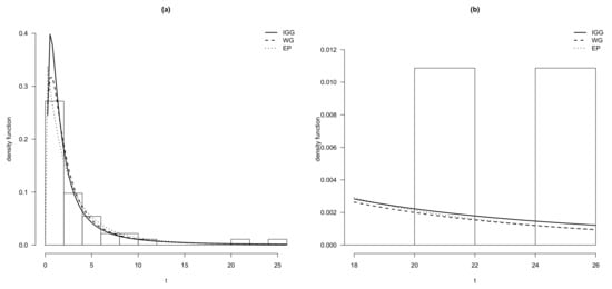
Figure 2. (a) Density function for IGG, WG and EP models and (b) for the right tail in repair times data set.

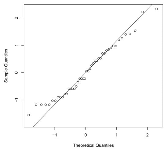
Figure 3. QQ-plot of the randomized quantile residuals of IGG distribution for repair times data set.

5.2. Gauge Lengths Data Set

The second data set was originally reported by Badar and Priest [24] and it also discussed in Kundu and Raqab [25]. It deals with the strength measured in GPA for single carbon fibers and impregnated 1000-carbon fiber tows. Single fibers were tested under tension at gauge lengths of 10 mm ($n=63$). The data set consists of the following observations: 1.901, 2.132, 2.203, 2.228, 2.257, 2.350, 2.361, 2.396, 2.397, 2.445, 2.454, 2.474, 2.518, 2.522, 2.525, 2.532, 2.575, 2.614, 2.616, 2.618, 2.624, 2.659, 2.675, 2.738, 2.740, 2.856, 2.917, 2.928, 2.937, 2.937, 2.977, 2.996, 3.030, 3.125, 3.139, 3.145, 3.220, 3.223, 3.235, 3.243, 3.264, 3.272, 3.294, 3.332. 3.346, 3.377, 3.408, 3.435, 3.493, 3.501, 3.537, 3.554, 3.562, 3.628, 3.852, 3.871, 3.886, 3.971, 4.024, 4.027, 4.225, 4.395, 5.020.

We use again the quantile-matching estimation method to find the estimates of the IGP, IGL and IGG distributions, obtaining $\theta =0.01$, $\alpha =20.1179$ and $\beta =58.5640$ for the IGP model, $\theta =0.01$, $\alpha =20.0862$ and $\beta =58.3896$ for the IGL model and $\theta =0.01$, $\alpha =20.0958$ and $\beta =58.5036$ for the IGG model respectively. Next, we estimate the parameters by means of the EM algorithm using those numbers as initial values. For the sake of model comparison, we have also fitted the WPS model, EG, EP and EL, respectively. Table 5 exhibits three measures of model selection, the maximum of the log-likelihood function (${\ell }_{max}$), AIC and BIC criteria, for the gauge lengths data set. Table 6 shows the estimates and standard errors (in brackets) for the three models of the EPS, WPS and IGPS families with a lower AIC and BIC statistics. Moreover, we propose again the use of the Anderson-Darling (AD) test statistics. We also are interested in testing for normality by means of the Shapiro–Francia (SF) and Shapiro–Wilk tests. For the AD test, smaller values of the test statistics indicate a better fit of the model to the data. With respect to the SF and SW tests under the null hypothesis the data are drawn from a normal distribution. As judged by the figures of p-value of the corresponding test statistics presented in Table 6, it can be seen that none of the models are rejected at the 5% significance level, validating that the models are statistically legitimate candidates to explain this data set. Once again, we have plotted in Figure 4 the histogram and the estimated density functions for this data set. Finally, the QQ-plot of the randomized quantile residuals is now displayed in Figure 5. It is again noticeable that the residuals for the IGG distribution underestimate the lower part and overestimate the upper part of the distribution of residuals.

Table 5. Maximum of the log-likelihood function ${\ell }_{max}$, AIC and BIC for EPS, WPS and IGPS models in the gauge lengths data set.

Model	${\mathit{\ell }}_{\mathit{max}}$	AIC	BIC
LL	−96.4058	196.8116	201.0979
LG	−59.4627	122.9254	127.2117
WP	−59.1711	124.3423	130.7717
WL	−61.2969	128.5939	135.0233
WG	−57.5006	121.0012	127.4306
IGP	−56.2875	118.5752	125.0046
IGL	−56.5613	119.1226	125.5520
IGG	−56.2871	118.5743	125.0037

Table 6. Estimates, standard errors (in brackets) and p-values associated with the AD, SF and SW statistics for IGG, WG and EP models in the gauge lengths data set.

Parameter	IGG	WG	LG
$\widehat{\theta }$	0.0102 (0.9237)	0.9717 (0.0429)	0.9997 (0.0003)
$\widehat{\alpha }$	26.0899 (4.9419)	8.3301 (1.0098)	3.0636 (0.2973)
$\widehat{\beta }$	76.6826 (13.8529)	4.6071 (0.6742)	—
p-value
AD	0.5279	0.2758	0.0954
SF	0.8328	0.4633	0.1339
SW	0.8874	0.4681	0.1096

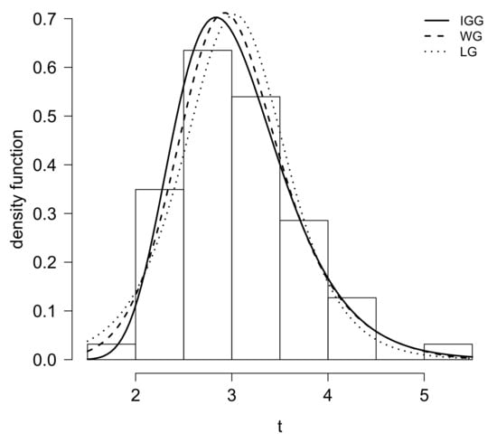
Figure 4. Density function for IGG, WG and LG models in gauge lengths data set.

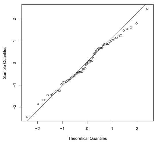
Figure 5. QQ-plot of the randomized quantile residuals of IGG distribution for gauge lengths data set.

6. Conclusions

In this paper, the inverse gamma power series (IGPS) family of probabilistic distribution has been introduced. This family has been obtained by mixing the inverse gamma and power series distributions. Moreover, four particular members of this family has been derived and examined. Some of its most relevant properties has been studied including the probability density function, survival and hazard functions, and the order statistics. The issue of parameter estimation was first discussed by means of the quantile-matching estimation method. Then, the estimates obtained by the latter method were used as initial values in a novel EM algorithm to carry out maximum likelihood estimation. Furthermore, a simulation study was performed to examine the efficiency of these estimates.

References

- Adamidis, K.; Loukas, S. A Lifetime Distribution with Decreasing Failure Rate. Stat. Probab. Lett. 1998, 39, 35–42. [Google Scholar] [CrossRef]
- Kus, C. A new lifetime distribution. Comput. Stat. Data Anal. 2007, 51, 4497–4509. [Google Scholar] [CrossRef]
- Tahmasbi, R.; Rezaei, S. A two-parameter lifetime distribution with decreasing failure rate. Comput. Stat. Data Anal. 2008, 52, 3889–3901. [Google Scholar] [CrossRef]
- Chahkandi, M.; Ganjali, M. On some lifetime distributions with decreasing failure rate. Comput. Stat. Data Anal. 2009, 53, 4433–4440. [Google Scholar] [CrossRef]
- Morais, A.L.; Barreto-Souza, W. A compound class of Weibull and power series distribution. Comput. Stat. Data Anal. 2011, 55, 1410–1425. [Google Scholar] [CrossRef]
- Mahmoudi, E.; Jafari, A.A. Generalized exponential power series distributions. Comput. Stat. Data Anal. 2012, 56, 4047–4066. [Google Scholar] [CrossRef]
- Silva, R.B.; Bourguignon, M.; Dias, C.R.B.; Cordeiro, G.M. The compound family of extended Weibull power series distributions. Comput. Stat. Data Anal. 2013, 58, 352–367. [Google Scholar] [CrossRef]
- Bagheri, S.F.; Samani, E.B.; Ganjali, M. The generalized modified Weibull power series distribution: Theory and applications. Comput. Stat. Data Anal. 2016, 94, 136–160. [Google Scholar] [CrossRef]
- Warahena-Liyanage, G.; Pararai, M. The Lindley Power Series Class of Distributions: Model. Properties and Applications. J. Comput. Model. 2015, 5, 35–80. [Google Scholar]
- Alizadeh, M.; Bagheri, S.F.; Bahrami-Samani, E.; Ghobadi, S.; Nadarajah, S. Exponentiated power Lindley power series class of distributions: Theory and applications. Commun.-Stat.-Simul. Comput. 2018, 47, 2499–2531. [Google Scholar] [CrossRef]
- Elbatal, I.; Zayedm, M.; Rasekhi, M.; Butt, N.S. The Exponential Pareto Power Series Distribution: Theory and Applications. Pak. J. Stat. Oper. Res. 2017, 13, 603–615. [Google Scholar] [CrossRef][Green Version]
- Elbatal, I.; Altun, E.; Afify, A.Z.; Ozel, G. The Generalized Burr XII Power Series Distributions with Properties and Applications. Ann. Data Sci. 2019, 6, 571–597. [Google Scholar] [CrossRef]
- Noack, A. On a class of discrete random variables. Ann. Math. Stat. 1950, 21, 127–132. [Google Scholar] [CrossRef]
- Patil, G.P. Certain Properties of the Generalized Power Series Distribution. Ann. Math. Stat. 1962, 21, 179–182. [Google Scholar] [CrossRef]
- Barakat, H.M.; Abdelkader, Y.H. Computing the moments of order statistics from nonidentical random variables. Stat. Methods Appl. 2004, 13, 15–26. [Google Scholar] [CrossRef]
- Dempster, A.P.; Laird, N.M.; Rubim, D.B. Maximum likelihood from incomplete data via the EM algorithm (with discussion). J. R. Stat. Soc. Ser. B 1977, 39, 1–38. [Google Scholar]
- Gallardo, D.I.; Romeo, J.S.; Meyer, R. A simplified estimation procedure based on the EM algorithm for the power series cure rate model. Commun. Stat.-Simul. Comput. 2017, 46, 6342–6359. [Google Scholar] [CrossRef]
- Meng, X.; Rubin, D. Maximum Likelihood Estimation via the ECM Algorithm: A General Framework. Biometrika 1993, 80, 267–278. [Google Scholar] [CrossRef]
- Louis, T. Finding the observed information matrix when using the EM algorithm. J. R. Stat. Soc. Ser. B 1982, 44, 226–233. [Google Scholar]
- Dunn, P.K.; Smyth, G.K. Randomized Quantile Residuals. J. Comput. Graph. Stat. 1996, 5, 236–244. [Google Scholar]
- Von Alven, W.H. Reliability Engineering by ARINC; Prentice Hall: Upper Saddle River, NJ, USA, 1964. [Google Scholar]
- Akaike, H. A new look at the statistical model identification. IEEE Trans. Autom. Control 1974, 19, 716–723. [Google Scholar] [CrossRef]
- Schwarz, G. Estimating the Dimension of a Model. Ann. Stat. 1978, 6, 461–464. [Google Scholar] [CrossRef]
- Badar, M.G.; Priest, A.M. Statistical aspects of fiber and bundle strength in hybrid composites. In Progress in Science and Engineering Composites; Hayashi, T., Kawata, K., Umekawa, S., Eds.; ICCM-IV: Tokyo, Japan, 1982; pp. 1129–1136. [Google Scholar]
- Kundu, D.; Raqab, M.Z. Estimation of R = P(Y < X) for three-parameter Weibull distribution. Stat. Probab. Lett. 2009, 79, 1839–1846. [Google Scholar]
Publisher’s Note: MDPI stays neutral with regard to jurisdictional claims in published maps and institutional affiliations. |
© 2021 by the authors. Licensee MDPI, Basel, Switzerland. This article is an open access article distributed under the terms and conditions of the Creative Commons Attribution (CC BY) license (https://creativecommons.org/licenses/by/4.0/).