Fault Diagnosis of Main Pump in Converter Station Based on Deep Neural Network

Abstract

As the core component of the valve cooling system in a converter station, the main pump plays a major role in ensuring the stable operation of the valve. Thus, accurate and efficient fault diagnosis of the main pump according to vibration signals is of positive significance for the detection of failure equipment and reducing the maintenance cost. This paper proposed a new neural network based on the vibration signals of the main pump to classify four faults and one normal state of the main pump, which consisted of a convolutional neural network (CNN) and long short-term memory (LSTM). Multi-scale features were extracted by two CNNs with different kernel sizes, and temporal features were extracted by LSTM. Moreover, random sampling was used in data processing for imbalanced data, which is meaningful for data symmetry. Experimental results indicated that the accuracy of the network was 0.987 obtained from the test set, and the average values of F1-score, recall, and precision were 0.987, 0.987, and 0.988, respectively. It was found that the proposed network performed well in a multi-label fault diagnosis of the main pump and was superior to other methods.

1. Introduction

The main pump, the core of the valve cooling system, is powered for the cooling system medium to ensure the converter valve work at a normal temperature through heat exchange, which can affect the safety and stability of HVDC and even threaten large-scale renewable power generation and load electrification [1,2]. Therefore, it has great practical significance for fault diagnosis of the main pump [3,4]. However, there are few studies on fault diagnosis of the main pump, and most of the existing methods are time-consuming and laborious. Therefore, it is urgent to develop an algorithm that can timely diagnose the state of the main pump with high accuracy.

Generally, the main pump is a horizontal centrifugal pump to undertake the power supply task, thus the main pump in this paper refers to the horizontal centrifugal pump [5]. In practical application, four faults and one normal state of the main pump appear most, namely unbalance, looseness, parallel misalignment (PM), angular misalignment (AM), and normal.

At present, two main methods have been applied for the fault diagnosis of the main pump, machine learning, and deep learning. The former is to extract the signal features manually and carry out fault diagnosis by machine learning methods, such as support vector machine (SVM), k-neighborhood algorithm (KNN), and so on. Kumar et al. [6] extracted the features from the original signal and scale edge integral graph, optimized the SVM parameters by genetic algorithm (GA), trained SVM with the optimal parameters, and classified the characteristics of the centrifugal pump. The classification accuracy can reach 96.66%. Ebrahimi et al. [7] decomposed the vibration signal in three levels by the Daubechies wavelet, and 44 descriptive statistical features were extracted from the detail coefficients and approximation coefficients of the wavelet. The SVM classifier with an accuracy of 96.67% was obtained. Hui et al. [8] proposed a time-frequency signal analysis method based on the theory of cyclostationary. Firstly, the cyclic autocorrelation function (CAFs) of various signals was calculated, and then the features of CAFs in the frequency domain were obtained by FFT, thus as to carry out the fault classification. Janani et al. [9] used a wrapper model to select the appropriate features from the power spectrum of vibration signal and line current signal in an induction motor. The features were input into a multi-class support vector machine (MSVM), and the optimal MSVM classifier was obtained by using the fivefold cross-validation to select the optimal Gaussian radial basis function (RBF) and MSVM parameters. Maamar et al. [10] combined multilayer perceptron with backward propagation (MLP-BP) and genetic algorithm (GA). The feature extraction was carried out by using continuous wavelet transform and three different wavelet functions, and then GA optimized the number of hidden layers and neurons of MLP-BP. Janani et al. [11] proposed two methods based on MSVM, best energy (BE) criterion, and principal component analysis (PCA). The current and vibration signals of motor were preprocessed by wavelet packet transform (WPT), and then the appropriate features were selected according to BE and PCA, and finally, the classification was completed by MSVM. Zahoor et al. [12] proposed a three-level fault diagnosis strategy. Firstly, the fault characteristic modes of vibration signals were identified and selected, and then the mixed features were extracted in the time domain, frequency domain, and time-frequency domain of vibration signals. Then, the high correlation features in mixed features were dimensioned and a new feature pool was formed by using Pearson linear discriminant analysis (PLDA). Finally, the fault classification was carried out by KNN. Zahoor et al. [13] used cross-correlation between health baseline signal and other kinds of signals to obtain new features from the correlation sequence. Then, they extracted the mixed features in time domain, frequency domain, and time-frequency domain from these features and formed feature vectors by calculating correlation coefficients between different signals. Finally, they input feature vectors into MSVM to implement fault diagnosis. The research on fault diagnosis of the main pump mostly adopts the above methods, but they are time-consuming and may cause mistakes due to human misinterpretation.

The latter is to preprocess the signal and extract features automatically through deep learning methods to implement fault diagnosis. Deep learning methods have been used in fault diagnosis of mechanical equipment because of their superior ability of automatic feature extraction, especially convolutional neural network (CNN) and recurrent neural network (RNN). Wang et al. [14] transformed the raw signal into a spectrum signal through discrete Fourier transform (DFT) and then stacked the spectrum signal as a sample to input into CNN. Guo et al. [15] proposed a hierarchical CNN network structure with an adaptive learning rate. The first layer was used to recognize the fault type of bearing. The second layer was used to evaluate the fault size in the bearing. Because the learning rate had a great impact on the network, they also proposed a method to obtain an adaptive learning rate for making an improvement on the training effect of the network. Zhang et al. [16] studied the rolling bearing fault in a noisy environment and under the condition of constantly changing workload and proposed a new CNN training method, which greatly improved the robustness of the network and maintained high accuracy and stability even in a noisy environment and under the condition of constantly changing workload. Kumar et al. [17] proposed an improved CNN. The gray image of the sound signal was obtained by processing the sound signal with the analytic wavelet function (AWT). They used a new divergence function based on entropy as the loss function of CNN to solve the overfitting problem of CNN. Considering the outstanding extraction ability for temporal features in fault diagnosis, RNN based fault diagnosis model has been widely developed. Talebi et al. [18] put forward the idea of dynamic modeling of RNN based wind turbines for solving the inevitable problem, which is the wind energy conversion system fault. The residual error was obtained by comparing the built model with the actual system output for improving the performance of the built model. Experiments showed that the scheme could quickly obtain the fault diagnosis results, and the diagnosis effect was very effective. Przystalka et al. [19] proposed a robust fault detection method based on RNN and chaotic engineering by using local RNN to learn the chaotic behavior of chaotic engineering system. Mrugalski et al. [20] optimized the dynamic nonlinear system, especially studied the robustness of fault diagnosis. The results output a set of fault diagnosis model to make an improvement on the robustness of RNN. The model was used to simulate the disturbance attenuation process of a dynamic nonlinear system, and the results showed that the system could improve the robustness of fault estimation. Although deep learning has made some achievements in the field of mechanical fault diagnosis with high efficiency, there are few pieces of research on the application of deep learning methods in main pump fault diagnosis. At the same time, CNN’s superior feature extraction ability and automatic feature extraction can get rid of the shortcomings of traditional fault diagnosis methods in manual feature extraction, but CNN cannot extract the temporal features of the signal. On the other hand, RNN can effectively extract the temporal features of signal, but its feature extraction ability is not as good as CNN in other aspects.

In order to solve the above problems, this paper proposed a fault diagnosis method based on Muti-scale Convolutional Neural Network and Long Short-Term Memory (MCNN-LSTM) hybrid neural network model for the main pump of valve cooling system in a converter station, and the performance of the model was evaluated by several indexes. This method takes into account the extraction of temporal and spatial features and retains the most features as far as possible, which makes this method more accurate than other methods. The experimental results showed that the method can diagnose the main pump quickly and accurately and had good generalizability. In this paper, Section 2 discusses the related works such as 1DCNN and LSTM. Section 3 introduces the construction and function of network in detail. Section 4 provides the composition and preprocessing of data. Section 5 describes the experiment and analyzes the results, and Section 6 draws a conclusion.

2. Related Work

2.1. One-Dimensional Convolutional Neural Network (1DCNN)

CNN is an efficient algorithm for image recognition. It is a deep feedforward neural network including convolution operation. CNN is highly invariant to translation, scaling, tilting, or other forms of deformation, thus it is mainly used to identify two-dimensional (2D) images with distortion invariance. CNN is commonly classified into 1DCNN and 2DCNN. 2DCNN is usually used for image feature extraction. 2D filter convolutes the data on the two-dimensional plane to extract features, but it will cause the loss of time features when processing time series data. The 1DCNN’s 1D filter will convolute along a single dimension, which can conserve the temporal features of the data. The vibration signal studied in this paper is 1D data and has obvious time characteristics, thus 1DCNN is used to extract data features. The convolution operation of 1DCNN’s convolution layer is as follows:

$$x_i^{l+1}(j)=K_i^l\times x^l(j)+b_i^l$$

(1)

where K and b are the weights and biases of the i-th filter of the l-st layer, respectively, and are the i-th local input of the l-th layer.

After the 1D convolution layer, the max-pooling layer is applied to decreasing the dimension and compressing the features, thus as to decrease the computational load of the model and extract the major features. The pooling operation of the max-pooling layer is as follows:

$$P_i^{l+1}(j)=\underset{(j-1)W+1\le t\le jW}{\max }\{q_i^l(t)\}$$

(2)

where q is the t-th neuron in the l-th layer of the i-th channel, and W is the width of the pooling kernel.

In this study, we also used the global average pooling (GAP) layer instead of the full connection layer to regularize the structure of the whole network, prevent over fitting, and directly give each channel the actual category meaning. The effect of the GAP was better than that of the full connection layer.

2.2. LSTM

RNN is a kind of network model with the characteristics of memory and parameter sharing, which can effectively process and predict sequence data. However, RNN has the situation of gradient disappearance and gradient explosion. For dealing with this problem, LSTM is proposed [21]. LSTM is an improved network based on traditional RNN, adding forget gate, input gate, and output gate. According to the hidden state of the upper layer, the forget gate adds weight to each input information through the sigmoid activation function, thus as to determine the retention and discard of information. The input gate uses the sigmoid activation function and the activation function to update the information, which determines how much information to update. The output gate determines what information is output. The three gates jointly control the updated state of the signal along the time axis to obtain the information of each time step. The update formula of the three doors is as follows:

$$f^t=\sigma (W^f{x}^t+V^i{h}^{t-1}+b^f)$$

(3)

$$i^t=\sigma (W^i{x}^t+V^i{h}^{t-1}+b^i)$$

(4)

$$o^t=\sigma (W^o{x}^t+V^o{h}^{t-1}+b^o)$$

(5)

$$c^t=f^t\odot c^{t-1}+i\odot \tanh (W^c{x}^t+V^c{h}^{t-1}+b^c)$$

(6)

$$h^t=o^t\odot \tanh (c^t)$$

(7)

where b is the deviation, W and V represent the input state weight and hidden state weight, respectively. In step t, forget gate f^t, input gate i^t, output gate o^t, and cell state c^t are updated by input x^t and hidden state.

3. The Proposed Model

3.1. The Framework of Proposed Model

The framework of the proposed MCNN-LSTM network is shown in Figure 1. To prevent the time sequence of data from being destroyed and extract multi-scale features of data, two 1DCNN with different sizes and number of cores were selected to implement feature extraction. Wide kernels CNN automatically extracts low-frequency features, and narrow kernels CNN automatically extracts high-frequency features. The features were fused after GAP, and the formed fusion features adjust the data distribution through the Batch Normalization (BN) layer [22], thus as to speed up the network training and convergence. Then the temporal features were extracted by two-layer LSTM. Finally, a softmax classifier was used for output classification. The network structure proposed in this paper was inspired by the traditional CNN-LSTM and GoogLeNet model, and some improvements have been made. The framework of network and data transmission is shown in Figure 1. The network parameters are shown in Table 1.

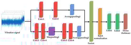
Figure 1. The framework of the proposed network. The network input is a 1024 × 3 matrix. The network output is a 1 × 5 vector obtained by the softmax function. The components of the network are 1D convolution layer, 1D pooling layer and LSTM.

Table 1. Proposed network parameters applied. The parameters of each layer, which contains the input layer, including the number of filters, kernel size, kernel stride, input and output size of each layer.

Name	Filters	Kernel Size/Stride	Units	Input Size	Output Size
Input					1024 × 3
Conv_1	50	36/2		1024 × 3	495 × 50
Conv_2	30	5/2		495 × 50	246 × 30
AveragePooling_1		2/2		246 × 30	123 × 30
Conv_3	50	7/1		1024 × 3	1018 × 50
Conv_4	40	7/1		1018 × 50	1012 × 40
Maxpooling_1		2/2		1012 × 40	506 × 40
Conv_5	30	7/1		506 × 40	500 × 30
Conv_6	30	7/2		500 × 30	247 × 30
Averagepooling_2		2/2		247 × 30	123 × 30
Batch_normalization_1				123 × 30	123 × 30
Lstm_1			60	123 × 30	123 × 60
Lstm_2			30	123 × 60	1 × 30
Dense			5	1 × 30	1 × 5

3.2. Model Setup

In this paper, the Adam algorithm [23] was used to update the parameters. The Adam algorithm can adjust the learning rate adaptively to make the training converge faster, and the learning rate was set to 0.006. Mean square error (MSE) was selected as a loss function.

4. Data

In order to make full use of the advantages of the deep neural network, a large quantity of data was needed to train the network. When the main circulating pump worked in different fault states, we collected the vibration signals from it, with a total of 1975,914 data points, and the amplitude of data was quite different. In order to facilitate neural network training, it was necessary to preprocess the data set first.

4.1. Data Description

The research object of this paper was the main pump of the water cooling system in the converter valve. The main pump was a NKG200-150-400/410 H1F2KE-SBQQE centrifugal pump. When sampling, the main pump speed was 2978 r/min, and the sampling frequency was 12 kHz. For obtaining the data of four different faults, we artificially caused four main pump failures. The data of normal, unbalance, looseness, parallel misalignment (PM), and angular misalignment (AM) were collected from the vertical, horizontal, and axial directions by vibration acceleration sensors. The experimental setup is shown in Figure 2. The data set containing five kinds of fault data is shown in Table 2. It can be found that the data set was characterized by serious imbalance. There were 317,031 points in each direction of PM and AM. However, the amount of data in normal, unbalanced, and looseness were only 8192 points in each direction.

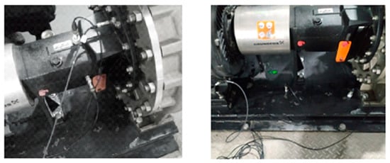
Figure 2. The experimental setup, centrifugal pump, and vibration acceleration sensors in vertical, horizontal, and axial directions.

Table 2. Detailed data volume of various states of data set, including parallel misalignment (PM), normal, unbalance, angular misalignment (AM), looseness.

Type	Vertical Direction	Horizontal Direction	Axial Direction
PM	317,031	317,031	317,031
Normal	8192	8192	8192
Unbalance	8192	8192	8192
AM	317,031	317,031	317,031
Looseness	8192	8192	8192

4.2. Data Processing

From Table 1, it can be found that the data were imbalanced. In order to solve this problem, a random sampling method [24,25,26,27] was used to enhance and balance the data set for data symmetry. Through the comprehensive analysis of the vibration signal, the sample length of each vibration signal was set at 1024 points, thus as to ensure the maximum information integrity of the sample in the case of the same sample length. As for the sample length, we compared different sample lengths in Section 5 to show the impact of sample length on the model performance. The data in three directions was taken as a sample for random sampling, and 1024 points in each direction were taken to form a 1000 × 1024 × 3 data set. To ensure effectiveness and robustness of proposed model, the data set was split into 70% for training and 30% for testing to obtain 700 training samples and 300 test samples.

Since the magnitude of the data was different, direct input of data into the model will increase the computational load of the network, affect the classification accuracy, and model convergence speed. Thus, standardizing the data was necessary. This paper used Z-Score standardization, which can unify data of different amplitude into the same magnitude. The specific formula is as follows:

$$z_{new}=\frac{z_{old}-\mu }{\delta }$$

(8)

where z_new stands for standardized data and z_old stands for original data. μ and δ are the mean and standard deviation of the data, respectively.

5. Results and Discussion

Because of the excellent performance of accuracy, recall, precision, and F1-score in the model evaluation, much literature have adopted these indicators as the evaluation criteria of the model. Therefore, this paper selected accuracy, recall, precision, and F1-score as evaluation indexes.

$$Accuracy=\frac{TP+TN}{TP+FP+FN+TN}$$

(9)

$$Recall=\frac{TP}{TP+FN}$$

(10)

$$Precision=\frac{TP}{TP+FP}$$

(11)

$$F1=\frac{2\times Precision\times Recall}{Precision+Recall}$$

(12)

where TP, TN, FP, and FN represent the number of true positive, true negative, false positive and false negative respectively.

5.1. Results Analysis

All the experiments in the study were completed with the Spyder (python3.6) compiler, run on a GTX950m graphics card, Intel Core i5 2.3 GHz processor, and a 4 GB RAM. The neural network was implemented under the Keras (2.0.8) framework with tensorflow backend. Some third-party libraries such as Sklearn, SciPy, and Matplotlib were used for data preprocessing and visualization.

We added two sets of comparative experiments to study the effect of sample length and RNN variables on model performance. Table 3 intuitively shows the experimental results of sample length on the test set from the aspects of data. In Table 3, the average values of evaluation indexes of each fault type were taken and arranged. It can be seen from Table 3 that the 1024-length sample has the best performance in F1-score and precision, which are basically above 0.95, and the comprehensive performance is also the best. The mean values of F1-score, recall, and precision decreased obviously with the decrease of sample length from 1024. When it increased from 1024, there was an obvious downward trend. Thus, 1024 was the most suitable sample length. We selected RNN variables including unidirectional LSTM, unidirectional gated recurrent unit (GRU) [28], bidirectional LSTM (BiLSTM) [29], and bidirectional GRU (BiGRU) [30]. Based on the 1024-length sample, the RNN variable comparison test was carried out. In Table 4, the LSTM performed well in F1-score and recall, but its advantage in precision was not obvious. The precision of LSTM was only slightly higher than that of BiLSTM, but LSTM was superior in other evaluation indexes, and the unidirectional network was superior to the bidirectional network, which was contrary to RNN commonly used in traditional text processing. We speculate that it may be caused by the change of the length and channel number of the data processed by CNN.

Table 3. The performance comparison for different sample lengths with the proposed model.

Evaluation Index	Length
	256	512	1024	2048	4096
F1-score	0.925	0.942	0.987	0.925	0.881
Recall	0.924	0.941	0.987	0.921	0.876
Precision	0.932	0.944	0.988	0.931	0.899
Accuracy	0.930	0.943	0.987	0.927	0.890

Table 4. The performance comparison for different RNN variables with the proposed model.

Evaluation Index	Module
	Unidirectional LSTM	Bidirectional LSTM	Unidirectional GRU	Bidirectional GRU
F1-score	0.987	0.909	0.883	0.849
Recall	0.987	0.908	0.883	0.849
Precision	0.988	0.970	0.890	0.951
Accuracy	0.987	0.910	0.883	0.840

5.2. Model Evaluation

The confusion matrix based on the best classification result of the test set is shown in Figure 3. From Figure 3, it is obvious that the learning outcome of the model is excellent. For obtaining a more objective and comprehensive evaluation of the model, we calculated the F1-score, recall, and precision on the test set, which is summarized in Table 5 below. It can be seen that all indexes of this model have high scores, stable performance, and strong generalization ability, and it has good performance for fault diagnosis.

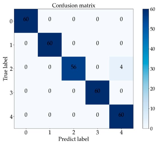
Figure 3. The confusion matrix of the fault diagnosis model on the test set. Tags 0–4 represent PM, normal, unbalance, AM and looseness, respectively.

Table 5. Evaluation index of fault diagnosis model on the test set.

Type	Evaluation Index
	F1 Score	Recall	Precision
PM	1.000	1.000	1.000
Normal	1.000	1.000	1.000
Unbalance	0.966	0.933	1.000
AM	1.000	1.000	1.000
Looseness	0.969	1.000	0.939
Average	0.987	0.987	0.988
Accuracy	0.987

5.3. Algorithm Comparison

There are many algorithms for fault diagnosis of vibration signals. We chose several machine learning algorithms and deep learning algorithms for comparative experiments. From Table 6, it can be found that our proposed model has a good performance in terms of F1-score, recall, precision, and accuracy, which is better than the comparison algorithm. The specific values of each index are shown in the table below.

Table 6. The proposed model was compared with other models.

Method	Evaluation Index
	F1 Score	Recall	Precision	Accuracy
Proposed	0.987	0.987	0.988	0.987
CNN	0.905	0.902	0.910	0.910
WDCNN	0.842	0.845	0.887	0.853
LSTM	0.769	0.766	0.854	0.817
BiLSTM	0.858	0.855	0.897	0.870
GRU	0.812	0.809	0.887	0.817
BiGRU	0.954	0.953	0.956	0.953
K-NN	0.336	0.438	0.491	0.457
Random Forest	0.642	0.650	0.562	0.660

5.4. Network Visualization

The inner part of the neural network model has always been considered as a black box, and the inner principle is difficult to understand. In this section, T-SNE was applied to visualizing the feature extraction process of internal network structure and exploring the internal feature extraction and classification process. First of all, from the input data, we selected the wide kernels CNN to preliminarily classify the data and distinguish PM, normal, and unbalance from AM and looseness. Then, narrow kernel CNN was used to subdivide AM and looseness. Through the first-layer LSTM, it can be preliminarily divided into three categories: PM, normal, and unbalance. On the basis of the first-layer LSTM, the boundaries of the five types of data were clearly divided with the second-layer LSTM. Finally, the data were divided into five categories by softmax. As shown in Figure 4, the feature distribution extracted in this paper has a very clear boundary, and the classification effect is very good.

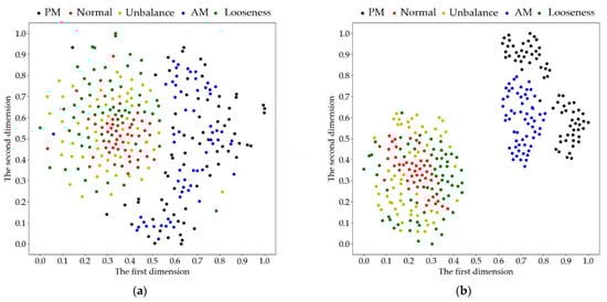
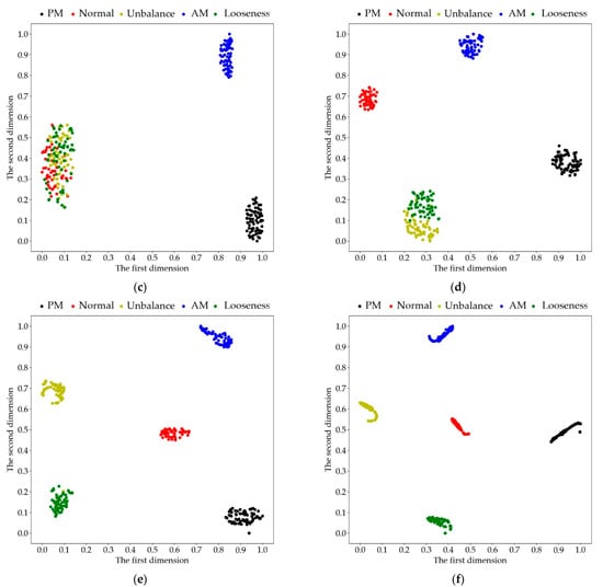
Figure 4. Feature visualization based on T-SNE. (a) Feature visualization of input signal, (b) output feature visualization of wide kernel CNN, (c) output feature visualization of narrow kernel CNN, (d) output feature visualization of first-layer LSTM, (e) output feature visualization of second-layer LSTM, (f) output feature visualization of softmax.

5.5. Future Work

According to some problems of the model, the future research focuses on the following three aspects. First of all, we need to improve the data preprocessing method and the network structure and achieve more accurate fault classification while reducing the network parameters as much as possible. Secondly, this study only realized the classification of four faults and one normal state. In the future, more vibration signals of other fault types will be collected to realize more fault classification. Finally, some other data enhancement methods will be tried, and a new fault diagnosis model is established by combining machine learning methods such as PCA with deep learning algorithms.

6. Conclusions

In this paper, the main innovation was to propose a new deep neural network combining CNN and LSTM, which can classify the vibration signals of the main pump directly. The influence and importance of sample length and RNN variable selection on the performance of the model was verified by comparison experiments. The experiments on the test set showed that the model has high scores in many indexes. The mean values of F1-score, recall, and precision were 0.987, 0.987, and 0.988, respectively, with an accuracy of 0.987. Finally, the feature extraction and classification process of the model were also visualized by T-SNE.

References

- Holweg, J.; Lips, H.P.; Tu, B.Q.; Uder, M.; Peng, B.; Zhang, Y. Modern HVDC thyristor valves for China’s electric power system. In Proceedings of the Proceedings. International Conference on Power System Technology, Kunming, China, 13–17 October 2002; Volume 521, pp. 520–527. [Google Scholar]
- Wen, Y.L.; Leng, M.Q.; Zhang, E.L.; Zhang, Z.G.; Chen, J.Y. Hybrid Cooling System for HVDC Convertor Valves. Appl. Mech. Mater. 2014, 3391, 588–595. [Google Scholar] [CrossRef]
- Qian, Y.H.; Zhou, Y.Y.; Xu, C.W. Research on the Formation and Preventive Measure of Scale in the Cooling System of HVDC Converter Valve. Adv. Mater. Res. 2012, 354, 1157–1160. [Google Scholar] [CrossRef]
- ShaoHua, Y.; Qibin, T.; Maozhong, W.; Luxiang, Z. Cooling System Circuit Analysis of ±800 kV DC Power Transmission Converter Valve. In Proceedings of the 2015 4th International Conference on Computer, Mechatronics, Control and Electronic Engineering, Hangzhou, China, 28–29 September 2015; pp. 1124–1127. [Google Scholar]
- Wu, A.; Guan, S.; Geng, M.; Cui, P. Fault analysis and optimized improvement for main pump of HVDC Converter Stations valve cooling system. In Proceedings of the 2020 4th International Conference on HVDC (HVDC), Xi’an, China, 6–9 November 2020. [Google Scholar]
- Kumar, A.; Kumar, R. Time-frequency analysis and support vector machine in automatic detection of defect from vibration signal of centrifugal pump. Measurement 2017, 108, 119–133. [Google Scholar] [CrossRef]
- Ebrahimi, E.; Javidan, M. Vibration-based classification of centrifugal pumps using support vector machine and discrete wavelet transform. J. Vibroeng. 2017, 19, 2586–2597. [Google Scholar] [CrossRef]
- Hui, S.; Yuan, S.; Yin, L. Cyclic Spectral Analysis of Vibration Signals for Centrifugal Pump Fault Characterization. IEEE Sens. J. 2018, 18, 2925–2933. [Google Scholar]
- Rapur, J.S.; Tiwari, R. Automation of multi-fault diagnosing of centrifugal pumps using multi-class support vector machine with vibration and motor current signals in frequency domain. J. Braz. Soc. Mech. Sci. Eng. 2018, 40, 278. [Google Scholar] [CrossRef]
- Al-Tubi, M.; Bevan, G.P.; Wallace, P.A.; Harrison, D.K.; Ramachandran, K.P. Fault diagnosis of a centrifugal pump using MLP-GABP and SVM with CWT. J. Eng. Sci. Technol. 2019, 22, 854–861. [Google Scholar]
- Rapur, J.S.; Tiwari, R. Experimental fault diagnosis for known and unseen operating conditions of centrifugal pumps using MSVM and WPT based analyses. Measurement 2019, 147, 106809. [Google Scholar] [CrossRef]
- Ahmad, Z.; Prosvirin, A.E.; Kim, J.; Kim, J. Multistage Centrifugal Pump Fault Diagnosis by Selecting Fault Characteristic Modes of Vibration and Using Pearson Linear Discriminant Analysis. IEEE Access 2020, 8, 223030–223040. [Google Scholar] [CrossRef]
- Ahmad, Z.; Rai, A.; Ma Liuk, A.S.; Kim, J.M. Discriminant Feature Extraction for Centrifugal Pump Fault Diagnosis. IEEE Access 2020, 8, 165512. [Google Scholar] [CrossRef]
- Wang, L.H.; Zhao, X.P.; Wu, J.X.; Xie, Y.Y.; Zhang, Y.H. Motor Fault Diagnosis Based on Short-time Fourier Transform and Convolutional Neural Network. Chin. J. Mech. Eng. 2017, 30, 1357–1368. [Google Scholar] [CrossRef]
- Guo, X.; Chen, L.; Shen, C. Hierarchical adaptive deep convolution neural network and its application to bearing fault diagnosis. Measurement 2016, 93, 490–502. [Google Scholar] [CrossRef]
- Wei, Z.; Li, C.; Peng, G.; Chen, Y.; Zhang, Z. A deep convolutional neural network with new training methods for bearing fault diagnosis under noisy environment and different working load. Mech. Syst. Signal Process. 2017, 100, 439–453. [Google Scholar]
- Kumar, A.; Gandhi, C.P.; Zhou, Y.; Kumar, R.; Xiang, J. Improved deep convolution neural network (CNN) for the identification of defects in the centrifugal pump using acoustic images. Appl. Acoust. 2020, 167, 107399. [Google Scholar] [CrossRef]
- Talebi, N.; Ali Sadrnia, M.; Darabi, A. Robust fault detection of wind energy conversion systems based on dynamic neural networks. Comput. Intell. Neurosci. 2014, 2014, 580972. [Google Scholar] [CrossRef] [PubMed] [Green Version]
- Przystałka, P.; Moczulski, W. Methodology of neural modelling in fault detection with the use of chaos engineering. Eng. Appl. Artif. Intell. 2015, 41, 25–40. [Google Scholar] [CrossRef]
- Mrugalski, M.; Luzar, M.; Pazera, M.; Witczak, M.; Aubrun, C. Neural network-based robust actuator fault diagnosis for a non-linear multi-tank system. ISA Trans. 2016, 61, 318–328. [Google Scholar] [CrossRef]
- Greff, K.; Srivastava, R.K.; Koutník, J.; Steunebrink, B.R.; Schmidhuber, J. LSTM: A Search Space Odyssey. IEEE Trans. Neural Netw. Learn. Syst. 2017, 28, 2222–2232. [Google Scholar] [CrossRef] [Green Version]
- Ioffffe, S.; Szegedy, C. Batch normalization: Accelerating deep network training by reducing internal covariate shift. arXiv 2015, arXiv:1502.03167. [Google Scholar]
- Kingma, D.P.; Ba, J. Adam: A method for stochastic optimization. arXiv 2014, arXiv:1412.6980. [Google Scholar]
- Yao, Z.; Yu, Y.; Yao, J. Artificial neural network–based internal leakage fault detection for hydraulic actuators: An experimental investigation. Proc. Inst. Mech. Eng. Part I J. Syst. Control. Eng. 2017, 232, 369–382. [Google Scholar] [CrossRef]
- Cheemala, V.; Asokan, A.N.; Preetha, P. Transformer Incipient Fault Diagnosis using Machine Learning Classifiers. In Proceedings of the 2019 IEEE 4th International Conference on Condition Assessment Techniques in Electrical Systems (CATCON), Chennai, India, 21–23 November 2019. [Google Scholar]
- Jin, G.; Zhu, T.; Akram, M.W.; Jin, Y.; Zhu, C. An Adaptive Anti-Noise Neural Network for Bearing Fault Diagnosis under Noise and Varying Load Conditions. IEEE Access 2020, 8, 74793–74807. [Google Scholar] [CrossRef]
- Chen, R.; Zhu, J.; Hu, X.; Wu, H.; Xu, X.; Han, X. Fault diagnosis method of rolling bearing based on multiple classifier ensemble of the weighted and balanced distribution adaptation under limited sample imbalance. ISA Trans. 2020, 114, 434–443. [Google Scholar] [CrossRef] [PubMed]
- Dey, R.; Salemt, F.M. Gate-variants of Gated Recurrent Unit (GRU) neural networks. In Proceedings of the 2017 IEEE 60th International Midwest Symposium on Circuits and Systems (MWSCAS), Boston, MA, USA, 6–9 August 2017. [Google Scholar]
- Yi, B.; Yang, Y.; Huang, Z.; Shen, F.; Shen, H.T. Bidirectional Long-Short Term Memory for Video Description. ACM 2016, 436–440. [Google Scholar] [CrossRef] [Green Version]
- Xie, X. Opinion Expression Detection via Deep Bidirectional C-GRUs. In Proceedings of the International Workshop on Database & Expert Systems Applications, Lyon, France, 28–31 August 2017. [Google Scholar]
Publisher’s Note: MDPI stays neutral with regard to jurisdictional claims in published maps and institutional affiliations. |
© 2021 by the authors. Licensee MDPI, Basel, Switzerland. This article is an open access article distributed under the terms and conditions of the Creative Commons Attribution (CC BY) license (https://creativecommons.org/licenses/by/4.0/).