Existence of Solutions for a Singular Fractional q-Differential Equations under Riemann–Liouville Integral Boundary Condition

Abstract

We investigate the existence of solutions for a system of m-singular sum fractional q-differential equations in this work under some integral boundary conditions in the sense of Caputo fractional q-derivatives. By means of a fixed point Arzelá–Ascoli theorem, the existence of positive solutions is obtained. By providing examples involving graphs, tables, and algorithms, our fundamental result about the endpoint is illustrated with some given computational results. In general, symmetry and q-difference equations have a common correlation between each other. In Lie algebra, q-deformations can be constructed with the help of the symmetry concept.

1. Introduction

There are many definitions of fractional derivatives that have been formulated according to two basic conceptions: one of a global (classical) nature and the other of a local nature. Under the first formulation, the fractional derivative is defined as an integral, Fourier, or Mellin transformation, which provides its non-local property with memory. The second conception is based on a local definition through certain incremental ratios. This global conception is associated with the appearance of the fractional calculus itself and dates back to the pioneering works of important mathematicians, such as Euler, Laplace, Lacroix, Fourier, Abel, and Liouville, until the establishment of the classical definitions of Riemann–Liouville and Caputo.

Until relatively recently, the study of these fractional integrals and derivatives was limited to a purely mathematical context; however, in recent decades, their applications in various fields of natural Sciences and technology, such as fluid mechanics, biology, physics, image processing, or entropy theory, have revealed the great potential of these fractional integrals and derivatives [1,2,3,4,5,6,7,8,9]. Furthermore, the study from the theoretical and practical point of view of the elements of fractional differential equations has become a focus for interested researchers [10,11,12,13,14,15].

The q-difference equations (qDifEqs) were first proposed by Jackson in 1910 [16]. After that, qDifEqs were investigated in various studies [17,18,19,20,21,22,23,24]. On the contrary, integro-differential equations (InDifEqs) have been recently studied via various fractional derivatives and formulations based on the original idea of qDifEqs (see [25,26,27,28,29,30,31,32]). The concept of symmetry and q-difference equations are connected to each other while theoretically investigating the differential equation symmetries.

The solution existence and uniqueness for the fractional qDifEqs were investigated in  2012 by Ahmad et al. as: ${}^c{\mathcal{D}}_q^{\alpha }\left[u\right]\left(t\right)=T\left(t,u\left(t\right)\right)$ with boundary conditions (B.Cs):

$${\alpha }_{1}u\left(0\right)-{\beta }_1{\mathcal{D}}_q\left[u\right]\left(0\right)={\gamma }_{1}u\left({\eta }_1\right),{\alpha }_{2}u\left(1\right)-{\beta }_2{\mathcal{D}}_q\left[u\right]\left(1\right)={\gamma }_{2}u\left({\eta }_2\right),$$

where $\alpha \in (1,2]$, ${\alpha }_i,{\beta }_i,{\gamma }_i$, ${\eta }_i$ are real numbers, for $i=1,2$ and $T\in C(J\times \mathbb{R},\mathbb{R})$ [20]. The q-integral problem was studied in in 2013 by Zhao et al. as:

$${\mathcal{D}}_q^{\alpha }\left[u\right]\left(t\right)+f(t,u\left(t\right))=0,$$

with B.Cs: $u\left(1\right)=\mu {\mathcal{I}}_q^{\beta }\left[u\right]\left(\eta \right)$ and $u\left(0\right)=0$ almost ∀$t\in (0,1)$, where $q\in (0,1)$, $\alpha \in (1,2]$, $\beta \in (0,2]$, $\eta \in (0,1)$, $\mu$ is positive real number, and ${\mathcal{D}}_q^{\alpha }$ is the q-derivative of Riemann–Liouville (RL) and the real values continuous map u defined on $I\times [0,\infty )$ [24]. The problem:

$${}^c{D}_q^{\beta }({}^c{D}_q^{\gamma }+\lambda )\left[u\right]\left(t\right)=pf(t,u\left(t\right))+k{\mathcal{I}}_q^{\xi }\left[g\right](t,u\left(t\right))$$

was investigated in 2014 by Ahmad et al. with B.Cs:

$${\alpha }_{1}u\left(0\right)-{\beta }_1\left(t^{(1-\gamma )}{\mathcal{D}}_q\left[u\right]\left(0\right)\right){|}_{t=0}={\sigma }_{1}u\left({\eta }_1\right)$$

and

$${\alpha }_{2}u\left(1\right)+{\beta }_2{\mathcal{D}}_q\left[u\right]\left(1\right)={\sigma }_{2}u\left({\eta }_2\right),$$

where $t,q\in [0,1]$, ${}^c{\mathcal{D}}_q^{\beta }$ is the Caputo fractional q-derivative (CpFqDr), $0<\beta ,\gamma \le 1$, ${\mathcal{I}}_q^{\xi }(.)$ represents the RL integral with $\xi \in (0,1)$, f and g are given continuous functions, $\lambda$ and $p,k$ are real constants, ${\alpha }_i,{\beta }_i,{\sigma }_i\in \mathbb{R}$ and ${\eta }_i\in (0,1)$ for $i=1,2$ [19]. The solutions’ existence was studied in 2019 by Samei et al. for some multi-term q-integro-differential equations with non-separated and initial B.Cs ([23]).

Inspired by all previous works, we investigate in this work the positive solutions for the singular fractional q-differential equation (SFqDEqs) as follows:

$${}^c{\mathcal{D}}_q^{\alpha }\left[u\right]\left(t\right)+h(t,u\left(t\right))=0,$$

(1)

with the B.Cs: $u\left(0\right)=0$, $cu\left(1\right)={\mathcal{I}}_q^{\gamma }\left[u\right]\left(1\right)$ and $u^{″}\left(0\right)=\cdots =u^{(n-1)}\left(0\right)=0$, where $t\in J=(0,1)$, ${\mathcal{I}}_q^{\gamma }\left[u\right]$ is the RL q-integral of order $\gamma$ for the given function: u, here $q\in J$, $c\ge 1$, $n=\left[\alpha \right]+1$, $\alpha \ge 3$, $\gamma \in [1,\infty )$, $2{\Gamma }_q\left(\gamma \right)\ge {\Gamma }_q\left(\alpha \right)$, $h:(0,1]\times [0,\infty )\to [0,\infty )$ is continuous, ${lim}_{t\to 0^{+}}h(t,.)=+\infty$ that is, h is singular at $t=0$, and ${}^c{\mathcal{D}}_q^{\alpha }$ represents the CpFqDr of order $\alpha$, $q\in J$.

This work is divided into the following: some essential notions and basic results of q-calculus are reviewed in Section 2. Our original important results are stated in Section 3. In Section 4, illustrative numerical examples are provided to validate the applicability of our main results.

2. Essential Preliminaries

Assume that $q\in (0,1)$ and $a\in \mathbb{R}$. Define ${\left[a\right]}_q=\frac{1-q^a}{1-q}$ [16]. The power function: ${(x-y)}_q^n$ with $n\in {\mathbb{N}}_0$ is written as:

$${(x-y)}_q^{\left(n\right)}=\prod _{k=0}^{n-1}(x-y{q}^k)$$

for $n\ge 1$ and ${(x-y)}_q^{\left(0\right)}=1$, where x and y are real numbers and ${\mathbb{N}}_0:=\left\{0\right\}\cup \mathbb{N}$ ([17]). In addition, for $\sigma \in \mathbb{R}$ and $a\ne 0$, we obtain:

$${(x-y)}_q^{\left(\sigma \right)}=x^{\sigma }\prod _{k=0}^{\infty }\frac{x-y{q}^k}{x-y{q}^{\sigma +k}}.$$

If $y=0$, then it is obvious that $x^{\left(\sigma \right)}=x^{\sigma }$. The q-Gamma function is expressed by

$${\Gamma }_q\left(z\right)=\frac{{(1-q)}^{(z-1)}}{{(1-q)}^{z-1}},$$

where $z\in \mathbb{R}\backslash \{0,-1,-2,\cdots \}$ ([16]). We know that ${\Gamma }_q(z+1)={\left[z\right]}_q{\Gamma }_q\left(z\right)$. The value of the q-Gamma function, ${\Gamma }_q\left(z\right)$, for input values q and z with counting the sentences’ number n in summation by simplification analysis. A pseudo-code is constructed for estimating q-Gamma function of order n. The q-derivative of function w, is expressed as:

$${\mathcal{D}}_q\left[w\right]\left(x\right)={\left(\frac{\mathrm{d}}{\mathrm{d}x}\right)}_{q}w\left(x\right)=\frac{w\left(x\right)-w\left(qx\right)}{(1-q)x}$$

and ${\mathcal{D}}_q\left[w\right]\left(0\right)={lim}_{x\to 0}{\mathcal{D}}_q\left[w\right]\left(x\right)$ ([17]). In addition, the higher order q-derivative of a function w is defined by ${\mathcal{D}}_q^n\left[w\right]\left(x\right)={\mathcal{D}}_q{\mathcal{D}}_q^{n-1}\left[w\right]\left(x\right)$ for all $n\ge 1$, where ${\mathcal{D}}_q^0\left[w\right]\left(x\right)=w\left(x\right)$ ([17,18]). The q-integral of a function f defined on $[0,b]$ is expressed as:

$${\mathcal{I}}_q\left[w\right]\left(x\right)={\int }_0^{x}w\left(s\right){\mathrm{d}}_{q}s=x(1-q)\sum _{k=0}^{\infty }{q}^{k}w\left(x{q}^k\right),$$

for $0\le x\le b$, provided that the series is absolutely convergent ([17,18]). If a in $[0,b]$, then we have:

$${\int }_a^{b}w\left(u\right){\mathrm{d}}_{q}u={\mathcal{I}}_q\left[w\right]\left(b\right)-{\mathcal{I}}_q\left[w\right]\left(a\right)=(1-q)\sum _{k=0}^{\infty }{q}^k\left[bw\left(b{q}^k\right)-aw\left(a{q}^k\right)\right],$$

if the series exists. The operator ${\mathcal{I}}_q^n$ is given by ${\mathcal{I}}_q^0\left[w\right]\left(x\right)=w\left(x\right)$ and ${\mathcal{I}}_q^n\left[w\right]\left(x\right)={\mathcal{I}}_q{\mathcal{I}}_q^{n-1}\left[w\right]\left(x\right)$ for $n\ge 1$ and $g\in C\left(\right[0,b\left]\right)$ ([17,18]). It is proven that ${\mathcal{D}}_q{\mathcal{I}}_q\left[w\right]\left(x\right)=w\left(x\right)$ and ${\mathcal{I}}_q{\mathcal{D}}_q\left[w\right]\left(x\right)=w\left(x\right)-w\left(0\right)$ whenever w is continuous at $x=0$ ([17,18]). The fractional RL type q-integral of the function w on J for $\sigma \ge 0$ is defined by ${\mathcal{I}}_q^0\left[w\right]\left(t\right)=w\left(t\right)$, and

$$\begin{array}{cc}\hfill {\mathcal{I}}_q^{\alpha }\left[w\right]\left(t\right)& =\frac{1}{{\Gamma }_q\left(\sigma \right)}{\int }_0^t{(t-qs)}^{(\sigma -1)}w\left(s\right){\mathrm{d}}_{q}s\hfill \\ \hfill & =t^{\sigma }{(1-q)}^{\sigma }\sum _{k=0}^{\infty }{q}^k\frac{{\prod }_{i=1}^{k-1}\left(1-q^{\sigma +i}\right)}{{\prod }_{i=1}^{k-1}\left(1-q^{i+1}\right)}w\left(t{q}^k\right),\hfill \end{array}$$

for $t\in J$ and $\sigma >0$ ([22,33]). In addition, the CpFqDr of a function w is expressed as:

$$\begin{array}{cc}\hfill {}^c{\mathcal{D}}_q^{\sigma }\left[w\right]\left(t\right)& ={\mathcal{I}}_q^{\left[\sigma \right]-\sigma }\left[{}^c{\mathcal{D}}_q^{\left[\sigma \right]}\left[w\right]\right]\left(t\right)\hfill \\ \hfill & =\frac{1}{{\Gamma }_q\left(\left[\sigma \right]-\alpha \right)}{\int }_0^t{(t-qs)}^{\left(\left[\sigma \right]-\sigma -1\right)}{}^c{\mathcal{D}}_q^{\left[\sigma \right]}\left[w\right]\left(s\right){\mathrm{d}}_{q}s\hfill \\ \hfill & =\frac{1}{t^{\sigma }{(1-q)}^{\sigma }}\sum _{k=0}^{\infty }{q}^k\frac{{\prod }_{i=1}^{k-1}\left(1-q^{i-\sigma }\right)}{{\prod }_{i=1}^{k-1}\left(1-q^{i+1}\right)}w\left(t{q}^k\right),\hfill \end{array}$$

(2)

where $t\in J$ and $\sigma >0$ ([22]). It is proven that

$${\mathcal{I}}_q^{\beta }\left[{\mathcal{I}}_q^{\sigma }\left[w\right]\right]\left(x\right)={\mathcal{I}}_q^{\sigma +\beta }\left[w\right]\left(x\right)\mathrm{and}{}^c{\mathcal{D}}_q^{\sigma }\left[{\mathcal{I}}_q^{\sigma }\left[w\right]\right]\left(x\right)=w\left(x\right),$$

where $\sigma ,\beta \ge 0$ ([22]).

Some essential notions and lemmas are now presented as follows: In our work, $L^1\left(\overline{J}\right)$ and $C_{\mathbb{R}}\left(\overline{J}\right)$ are denoted by $\overline{\mathcal{L}}$ and $\overline{\mathcal{B}}$, respectively, where $\overline{J}=[0,1]$.

Lemma 1

([34]). If $x\in \overline{\mathcal{B}}\cap \overline{\mathcal{L}}$ with ${\mathcal{D}}_q^{\alpha }x\in \mathcal{B}\cap \mathcal{L}$, then

$${\mathcal{I}}_q^{\alpha }{\mathcal{D}}_q^{\alpha }x\left(t\right)=x\left(t\right)+\sum _{i=1}^n{c}_i{t}^{\alpha -i},$$

where n is the smallest integer $\ge \alpha$, and $c_i$ is some real number.

Here, we restate the well-known Arzelá–Ascoli theorem. Assume that $S={\left\{s_n\right\}}_{n\ge 1}$ is a sequence of bounded and equicontinuous real valued functions on $[a,b]$. Then, S has a uniformly convergent subsequence. We need the following fixed point theorem in our main result:

Lemma 2

([35]). Assume that $\mathcal{A}$ is a Banach space, $P\subseteq \mathcal{A}$ is a cone, and ${\mathcal{O}}_1$, ${\mathcal{O}}_2$ are two bounded open balls of $\mathcal{A}$ centered at the origin with ${\overline{\mathcal{O}}}_1\subset {\mathcal{O}}_2$. Assume that $\Omega :P\cap ({\overline{\mathcal{O}}}_2\backslash {\mathcal{O}}_1)\to P$ is a completely continuous operator such that either $\parallel \Omega \left(a\right)\parallel \le \parallel a\parallel$ for all $a\in P\cap \partial {\mathcal{O}}_1$ and $\parallel \Omega \left(a\right)\parallel \ge \parallel a\parallel$ for all $a\in P\cap \partial {\mathcal{O}}_2$, or $\parallel \Omega \left(a\right)\parallel \ge \parallel a\parallel$ for each $a\in P\cap \partial {\mathcal{O}}_1$ and $\parallel \Omega a\parallel \le \parallel a\parallel$ for $a\in P\cap \partial {\mathcal{O}}_2$. Then, Ω has a fixed point in $P\cap ({\mathcal{O}}_2\backslash {\mathcal{O}}_1)$.

3. Main Results

Differential Equation

Let us now present our fundamental lemma as follows:

Lemma 3.

The $u_0$ is a solution for the q-differential equation ${\mathcal{D}}_q^{\alpha }\left[u\right]\left(t\right)+g\left(t\right)=0$ with the B.Cs: $u\left(0\right)=0$, $cu\left(1\right)={\mathcal{I}}_q^{\gamma }u\left(1\right)$ and $u^{″}\left(0\right)=\cdots =u^{(n-1)}\left(0\right)=0$ if $u_0$ is a solution for the q-integral equation

$$u\left(t\right)={\int }_0^1{G}_q(t,s)f\left(s\right){\mathrm{d}}_{q}s,$$

where

$$G_q(t,s)=\left\{\begin{array}{cc}{\displaystyle \frac{-{(t-qs)}^{(\alpha -1)}}{{\Gamma }_q\left(\alpha \right)}}\hfill & s\le t,\hfill \\ +t^2{\displaystyle \frac{{\Gamma }_q(\gamma +3)\left[a{\Gamma }_q(\alpha +\gamma ){(1-qs)}^{(\alpha -1)}-{\Gamma }_q\left(\alpha \right){(1-qs)}^{(c+\gamma -1)}\right]}{{\Gamma }_q\left(\alpha \right){\Gamma }_q(\alpha +\gamma )\left[c{\Gamma }_q(\gamma +3)-2{\Gamma }_q\left(\gamma \right)\right]}},\hfill & \\ \hfill & \\ t^2{\displaystyle \frac{{\Gamma }_q(\gamma +3)\left[c{\Gamma }_q(\alpha +\gamma ){(1-qs)}^{(\alpha -1)}-{\Gamma }_q\left(\alpha \right){(1-qs)}^{(c+\gamma -1)}\right]}{{\Gamma }_q\left(\alpha \right){\Gamma }_q(\alpha +\gamma )\left[c{\Gamma }_q(\gamma +3)-2{\Gamma }_q\left(\gamma \right)\right]}},\hfill & t\le s,\hfill \end{array}\right.$$

(3)

for $s,t\in \overline{J}$, $n=\left[\alpha \right]+1$, the function $g\in \overline{\mathcal{B}}$, $\alpha \ge 3$ and $\gamma \in [1,\infty )$ with $2{\Gamma }_q\left(\gamma \right)\ge {\Gamma }_q\left(\alpha \right)$.

Proof. 

Let us first assume that $u_0$ is a solution for the equation ${\mathcal{D}}_q^{\alpha }u\left(t\right)+g\left(t\right)=0$ with the B.Cs. By using Lemma 1, we obtain:

$$u_0\left(t\right)=-{\mathcal{I}}_q^{\alpha }\left[g\right]\left(t\right)+c_0+c_{1}t+c_2{t}^2+\dots c_{n-1}{t}^{n-1}$$

and by using the condition $u_0\left(0\right)=u_0^{″}\left(0\right)=\cdots =u_0^{(n-1)}\left(0\right)=0$, we have

$$u_0\left(t\right)=-{\mathcal{I}}_q^{\alpha }\left[g\right]\left(t\right)+c_2{t}^2.$$

Indeed,

$${\mathcal{I}}_q^{\gamma }\left[u_0\right]\left(t\right)=-{\mathcal{I}}_q^{\alpha +\gamma }\left[g\right]\left(t\right)+c_2\frac{2{\Gamma }_q\left(\gamma \right)}{{\Gamma }_q(\gamma +3)}{t}^{\gamma +2},$$

and thus

$${\mathcal{I}}_q^{\gamma }\left[u_0\right]\left(1\right)=-{\mathcal{I}}_q^{(\alpha +\gamma )}\left[g\right]\left(t\right)+c_2\frac{2{\Gamma }_q\left(\gamma \right)}{{\Gamma }_q(\gamma +3)}.$$

Note that $c{u}_0\left(1\right)=-c{\mathcal{I}}_q^{\alpha }\left[g\right]\left(1\right)+c{c}_2$ and

$$\begin{array}{cc}\hfill c_2\left(c-\frac{2{\Gamma }_q\left(\gamma \right)}{{\Gamma }_q(\gamma +3)}\right)& =c{\mathcal{I}}_q^{\alpha }g\left(1\right)-{\mathcal{I}}_q^{\alpha +\gamma }g\left(1\right)\hfill \\ \hfill & =\frac{c{\Gamma }_q(\alpha +\gamma )}{{\Gamma }_q(\alpha +\gamma )}{\mathcal{I}}_q^{\alpha }\left[g\right]\left(1\right)-\frac{{\Gamma }_q\left(\alpha \right)}{{\Gamma }_q\left(\alpha \right)}{\mathcal{I}}_q^{\alpha +\gamma }\left[g\right]\left(1\right)\hfill \\ \hfill & ={\int }_0^1\frac{c{\Gamma }_q(\alpha +\gamma ){(1-qs)}^{(\alpha -1)}-{\Gamma }_q\left(\alpha \right)(1-q{s}^{(\alpha +\gamma -1)})}{{\Gamma }_q\left(\alpha \right){\Gamma }_q(\alpha +\gamma )}g\left(s\right){\mathrm{d}}_{q}s.\hfill \end{array}$$

On the other hand,

$$c-\frac{2{\Gamma }_q\left(\gamma \right)}{{\Gamma }_q(\gamma +3)}=\frac{c{\Gamma }_q(\gamma +3)-2{\Gamma }_q\left(\gamma \right)}{{\Gamma }_q(\gamma +3)}.$$

Hence,

$$c_2={\int }_0^1\frac{{\Gamma }_q(\gamma +3)\left[c{\Gamma }_q(\alpha +\gamma ){(1-qs)}^{(\alpha -1)}-{\Gamma }_q\left(\alpha \right){(1-qs)}^{(\alpha +\gamma -1)}\right]}{{\Gamma }_q\left(\alpha \right){\Gamma }_q(\alpha +\gamma )\left[c{\Gamma }_q(\gamma +3)-2{\Gamma }_q\left(\gamma \right)\right]}g\left(s\right){\mathrm{d}}_{q}s.$$

Therefore, we have

$$\begin{array}{cc}\hfill u_0\left(t\right)& =-{\mathcal{I}}_q^{\alpha }\left[g\right]\left(t\right)\hfill \\ \hfill & +t^2{\int }_0^1\frac{\Gamma (\gamma +3)\left[c{\Gamma }_q(\alpha +\gamma ){(1-qs)}^{(\alpha -1)}-{\Gamma }_q\left(\alpha \right){(1-qs)}^{(\alpha +\gamma -1)}\right]}{{\Gamma }_q\left(\alpha \right){\Gamma }_q(\alpha +\gamma )\left[c{\Gamma }_q(\gamma +3)-2{\Gamma }_q\left(\gamma \right)\right]}g\left(s\right){\mathrm{d}}_{q}s\hfill \\ \hfill & ={\int }_0^1{G}_q(s,t)g\left(s\right){\mathrm{d}}_{q}s,\hfill \end{array}$$

where

$$\begin{array}{cc}\hfill G_q(t,s)& =\frac{-{(t-qs)}^{(\alpha -1)}}{{\Gamma }_q\left(\alpha \right)}\hfill \\ \hfill & +t^2\frac{{\Gamma }_q(\gamma +3)\left[c{\Gamma }_q(\alpha +\gamma ){(1-qs)}^{(\alpha -1)}-{\Gamma }_q\left(\alpha \right){(1-qs)}^{c+\gamma -1}\right]}{{\Gamma }_q\left(\alpha \right){\Gamma }_q(\alpha +\gamma )\left[c{\Gamma }_q(\gamma +3)-2{\Gamma }_q\left(\gamma \right)\right]},\hfill \end{array}$$

whenever $0\le s\le t\le 1$ and

$$t^2\frac{{\Gamma }_q(\gamma +3)\left[c{\Gamma }_q(\alpha +\gamma ){(1-qs)}^{(\alpha -1)}-{\Gamma }_q\left(\alpha \right){(1-qs)}^{(c+\gamma -1)}\right]}{{\Gamma }_q\left(\alpha \right){\Gamma }_q(\alpha +\gamma )\left[c{\Gamma }_q(\gamma +3)-2{\Gamma }_q\left(\gamma \right)\right]}$$

whenever $0\le t\le s\le 1$. Hence, $u_0$ is an integral equation’s solution. By simple review, we can see that $u_0$ is a solution for the equation ${\mathcal{D}}_q^{\alpha }u\left(t\right)+g\left(t\right)=0$ with the B.Cs whenever $u_0$ is an integral equation’s solution. □

Remark 1.

By applying some simple calculations, one can show that $G_q(t,s)\ge 0$ for each $s,t\in \overline{J}$. Now, let us define the operator Ω on the Banach space $\overline{\mathcal{B}}$ by

$$\Omega \left(u\left(t\right)\right)={\int }_0^1{G}_q(t,s)h(s,u\left(s\right)){\mathrm{d}}_{q}s.$$

It is easy to check that $u_0$ is a fixed point of the operator Ω if $u_0$ is a solution for Equation (1).

Consider $\overline{\mathcal{B}}$ together the supremum norm and cone, P is the set of all $u\in \overline{\mathcal{B}}$ such that $u\left(t\right)\ge 0$∀$t\in \overline{J}$. Suppose that $h:(0,1]\times [0,\infty )\to [0,\infty )$ is the singular function at $t=0$ in the Equation (1) and $G_q(t,s)$ is the q-Green function in Lemma 3. Now, define the self operator $\Omega$ on P by

$$\Omega \left(u\left(t\right)\right)={\int }_0^1{G}_q(t,s)h(s,u\left(s\right)){\mathrm{d}}_{q}s,$$

for all $t\in \overline{J}$. At present, we can provide our first main result on the solution’s existence for problem (1) under some assumptions.

Theorem 1. 

Problem (1) has a unique solution if the following conditions hold.

I. 

There exists a continuous function $h:(0,1]\times [0,\infty )\to [0,\infty )$ such that

$$\underset{t\to 0^{+}}{lim}h(t,s)=\infty ,$$

for $s\in [0,\infty )$.

II. 

There exists $L>0$, $\beta \in J$ and positive constant k such that

$$kc{\Gamma }_q(\gamma +3)<(c{\Gamma }_q(\gamma +3)-2{\Gamma }_q\left(\gamma \right)),$$

$|t^{\beta }h(t,0)|\le L$ for each $t\in \overline{J}$ and

$$|t^{\beta }h(t,u\left(t\right))-t^{\beta }h(t,v\left(t\right))|\le k\parallel u-v\parallel ,$$

for each u, v belang to P.

Proof. 

Note that,

$$\left|\Omega \left(u\right(t\left)\right)\right|\le t^2\frac{c{\Gamma }_q(\gamma +3)}{c{\Gamma }_q(\gamma +3)-2{\Gamma }_q\left(\gamma \right)}{\mathcal{I}}_q^{\alpha }\left[h\right](1,u\left(1\right))$$

for all $t\in \overline{J}$. Now, put

$$\ell =L\frac{c{\Gamma }_q(\gamma +3){\Gamma }_q(1-\beta )}{c{\Gamma }_q(\gamma +3)-2{\Gamma }_q\left(\gamma \right)}$$

and define $B=\left\{u\in P:\parallel u\parallel \le \ell \right\}$. Clearly, B is a bounded and closed subset of $\mathcal{A}$, and thus B is complete. If $u\in B$, then we obtain:

$$|\Omega \left(u\left(t\right)\right)|\le \frac{c{\Gamma }_q(\gamma +3)}{{\Gamma }_q\left(\alpha \right)\left[c\Gamma (\gamma +3)-2{\Gamma }_q\left(\gamma \right)\right]}{\int }_0^1{(1-qs)}^{(\alpha -1)}{s}^{-\beta }{s}^{\beta }h(s,u\left(s\right)){\mathrm{d}}_{q}s$$

∀$t\in \overline{J}$ and thus

$$\begin{array}{cc}\hfill \left|F\right(x\left(t\right)\left)\right|& \le \frac{c{\Gamma }_q(\gamma +3)}{{\Gamma }_q\left(\alpha \right)\left[c{\Gamma }_q(\gamma +3)-2{\Gamma }_q\left(\gamma \right)\right]}\hfill \\ \hfill & \times {\int }_0^1{(1-qs)}^{(\alpha -1)}{s}^{-\beta }{s}^{\beta }\left(\left|h\right(s,u\left(s\right)-h(s,0)|+|h(s,0)|\right){\mathrm{d}}_{q}s\hfill \\ \hfill & \le (k\ell +L)\frac{c{\Gamma }_q(\gamma +3)}{{\Gamma }_q\left(\alpha \right)\left[c{\Gamma }_q(\gamma +3)-2{\Gamma }_q\left(\gamma \right)\right]}{B}_q(1-\beta ,\alpha )\hfill \\ \hfill & =(k\ell +L)\frac{c\Gamma (\gamma +3){\Gamma }_q(1-\beta )}{\left[c{\Gamma }_q(\gamma +3)-2{\Gamma }_q\left(\gamma \right)\right]{\Gamma }_q(\alpha -\beta +1)}\hfill \\ \hfill & \le \frac{\left[c{\Gamma }_q(\gamma +3)-2{\Gamma }_q\left(\gamma \right)\right]\ell }{c{\Gamma }_q(\gamma +s){\Gamma }_q(1-\beta )}\left[\frac{c{\Gamma }_q(\gamma +3){\Gamma }_q(1-\beta )}{(c{\Gamma }_q(\gamma +3)-2{\Gamma }_q\left(\gamma \right)){\Gamma }_q(\alpha -\beta +1)}\right]\hfill \\ \hfill & +L\frac{c{\Gamma }_q(\gamma +3){\Gamma }_q(1-\beta )}{\left[c{\Gamma }_q(\gamma +3)-2{\Gamma }_q\left(\gamma \right)\right]{\Gamma }_q(\alpha -\beta +1)}\hfill \\ \hfill & =\frac{\ell }{{\Gamma }_q(\alpha -\beta +1)}+\frac{\ell }{{\Gamma }_q(\alpha -\beta +1)}\hfill \\ \hfill & <\frac{\ell }{{\Gamma }_q\left(\alpha \right)}+\frac{\ell }{{\Gamma }_q\left(\alpha \right)}\le \frac{\ell }{2}+\frac{\ell }{2}=\ell .\hfill \end{array}$$

Indeed, $\Omega \left(B\right)\subseteq B$, and therefore a restriction of $\Omega$ on B is an operator on B. Let u, $v\in B$. Then, we obtain

$$\begin{array}{cc}\hfill \parallel \Omega \left(u\right(t\left)\right)-\Omega \left(v\right(t\left)\right)\parallel & \le \frac{1}{{\Gamma }_q\left(\alpha \right)}{\int }_0^1{(t-qs)}^{(\alpha -1)}\left|h(s,u(s\left)\right)-h(s,v(s)\right|{\mathrm{d}}_{q}s\hfill \\ \hfill & +\frac{c{t}^2{\Gamma }_q(\gamma +3)}{{\Gamma }_q\left(\alpha \right)\left[c{\Gamma }_q(\gamma +3)-2{\Gamma }_q\left(\gamma \right)\right]}\hfill \\ \hfill & \times {\int }_0^1{(1-qs)}^{(\alpha -1)}{s}^{-\beta }{s}^{\beta }\parallel h(s,u\left(s\right))-h(s,v\left(s\right))\parallel {\mathrm{d}}_{q}s\hfill \\ \hfill & \le k\parallel u-v\parallel \hfill \\ \hfill & \times \left[\frac{{\Gamma }_q(1-\beta )}{{\Gamma }_q(\alpha -\beta +1)}+\frac{c{\Gamma }_q(\gamma +3){\Gamma }_q(1-\beta )}{\left[c{\Gamma }_q(\gamma +3)-2{\Gamma }_q\left(\gamma \right)\right]{\Gamma }_q(\alpha -\beta +1)}\right]\hfill \\ \hfill & \le \left[\frac{c{\Gamma }_q(\gamma +3)-2{\Gamma }_q\left(\gamma \right)}{c{\Gamma }_q(\gamma +3){\Gamma }_q(\alpha -\beta +1)}+\frac{1}{{\Gamma }_q(\alpha -\beta +1)}\right]\parallel u-v\parallel \hfill \\ \hfill & <\left[\frac{c{\Gamma }_q(\gamma +3)-2{\Gamma }_q\left(\gamma \right)}{c{\Gamma }_q(\gamma +3){\Gamma }_q\left(\alpha \right)}+\frac{1}{{\Gamma }_q\left(\alpha \right)}\right]\parallel u-v\parallel \hfill \end{array}$$

for all $t\in \overline{J}$. Take

$$\lambda =\frac{c{\Gamma }_q(\omega +3)-2{\Gamma }_q\left(\omega \right)}{c{\Gamma }_q(\omega +3){\Gamma }_q\left(\alpha \right)}+\frac{1}{{\Gamma }_q\left(\alpha \right)}.$$

Since $\alpha \ge 3$, we obtain $\lambda \in J$, and therefore $\Omega :B\to B$ is a contraction. Thus, $\Omega$ has a unique fixed point in B. By employing Lemma 3, the problem (1) has a unique solution in B. □

Lemma 4.

Suppose that there exists $\beta \in J$ such that the map $t^{\beta }g\left(t\right)$ is a continuous map on J. If $G_q(t,s)$ is the q-Green function (3) in Lemma 3, then

$$\Omega \left(t\right)={\int }_0^1{G}_q(t,s)g\left(s\right){\mathrm{d}}_{q}s,$$

is also a continuous map on J. The self-operator Ω is completely continuous whenever there exists $\beta \in J$ such that the map $t^{\beta }g\left(t\right)$ is a continuous map on $\overline{J}$.

Proof. 

Since the map $t^{\beta }g\left(t\right)$ is continuous and $\Omega \left(t\right)={\int }_0^t{G}_q(t,s)s^{-\beta }{s}^{\beta }g\left(s\right){\mathrm{d}}_{q}s$, we obtain

$$\begin{array}{cc}\hfill |\Omega (t\left)\right|& \le \underset{s\in \delta }{sup}\left|G_q(t,s)s^{\beta }g\left(s\right)\right|{\int }_0^t{s}^{-\beta }\mathrm{d}s=\frac{m{t}^{1-\beta }}{1-\beta },\hfill \end{array}$$

where $\delta =[0,t]$,

$$m=\underset{s\in \delta }{sup}\left|G_q(t,s)s^{\beta }g\left(s\right)\right|<\infty .$$

Indeed, $\Omega \left(0\right)=0$. Note that, $G_q(t,s)$ is continuous in ${\overline{J}}^2$. First, suppose that $t_1=0$ and $t_2\in (0,1]$. By continuity $t^{\beta }g\left(t\right)$, there exists $L>0$ such that

$$\underset{t\in \overline{J}}{sup}\left|t^{\beta }g\left(t\right)\right|\le L.$$

Thus, we have:

$$\begin{array}{cc}\hfill |\Omega \left(t_2\right)-\Omega \left(t_1\right)|=|\Omega \left(t_2\right)|& \le {\int }_0^{t_2}\frac{{(1-qs)}^{(\alpha -1)}}{{\Gamma }_q\left(\alpha \right)}{s}^{-\beta }{s}^{\beta }g\left(s\right){\mathrm{d}}_{q}s\hfill \\ \hfill & +t_2^2{\int }_0^1\frac{{\Gamma }_q(\gamma +3)\left[c{\Gamma }_q(\alpha +\gamma )+{\Gamma }_q\left(\alpha \right)\right]}{{\Gamma }_q\left(\alpha \right)\left[c{\Gamma }_q(\gamma +3)-2{\Gamma }_q\left(\gamma \right)\right]}{(1-qs)}^{(\alpha -1)}{s}^{-\beta }{s}^{\beta }g\left(s\right){\mathrm{d}}_{q}s\hfill \\ \hfill & \le \frac{L}{{\Gamma }_q\left(\alpha \right)}{B}_q(1-\beta ,\alpha )t_2^{\alpha -\beta }\hfill \\ \hfill & +L{t}_2^2\frac{{\Gamma }_q(\gamma +3)\left[c{\Gamma }_q(\alpha +\gamma )+{\Gamma }_q\left(\alpha \right)\right]}{{\Gamma }_q\left(\alpha \right)\left[c{\Gamma }_q(\gamma +3)-2{\Gamma }_q\left(\gamma \right)\right]}{B}_q(1-\beta ,\alpha )\hfill \\ \hfill & =\frac{L{\Gamma }_q(1-\beta )}{{\Gamma }_q(\alpha -\beta +1)}{t}_2^{\alpha -\beta }\hfill \\ \hfill & +L\frac{{\Gamma }_q(\gamma +3){\Gamma }_q(1-\beta )\left[c{\Gamma }_q(\alpha +\gamma )+{\Gamma }_q\left(\alpha \right)\right]}{\left[c{\Gamma }_q(\gamma +3)-2{\Gamma }_q\left(\gamma \right)\right]{\Gamma }_q(\alpha -\beta +1)}{t}_2^2.\hfill \end{array}$$

This implies that ${lim}_{t_2\to t_1}|\Omega \left(t_2\right)-\Omega \left(t_1\right)|=0$. At present, in the next case, we assume that $t_1\in J$ and $t_2\in (t_1,1]$. Thus, we obtain:

$$\begin{array}{cc}\hfill |\Omega \left(t_2\right)-\Omega \left(t_1\right)|& \le \frac{1}{{\Gamma }_q\left(\alpha \right)}|-{\int }_0^{t_2}{(t_2-qs)}^{(\alpha -1)}{s}^{-\beta }{s}^{\beta }g\left(s\right){\mathrm{d}}_{q}s\hfill \\ \hfill & +{\int }_0^{t_1}{(t_1-qs)}^{(\alpha -1)}{s}^{-\beta }{s}^{\beta }g\left(s\right){\mathrm{d}}_{q}s|\hfill \\ \hfill & +|t_2^2-t_1^2|\frac{{\Gamma }_q(\gamma +3)\left[c{\Gamma }_q(\gamma +3)+{\Gamma }_q\left(\alpha \right)\right]}{{\Gamma }_q\left(\alpha \right)\left[c\Gamma (\gamma +3)-2{\Gamma }_q\left(\gamma \right)\right]}\hfill \\ \hfill & \times {\int }_0^1{(1-qs)}^{(\alpha -1)}{s}^{-\beta }{s}^{\beta }g\left(s\right){\mathrm{d}}_{q}s.\hfill \end{array}$$

On the other hand,

$$\begin{array}{cc}\hfill \frac{1}{{\Gamma }_q\left(\alpha \right)}& |-{\int }_0^{t_2}{(t_2-qs)}^{(\alpha -1)}{s}^{-\beta }{s}^{\beta }g\left(s\right){\mathrm{d}}_{q}s+{\int }_0^1{(t_1-qs)}^{(\alpha -1)}{s}^{-\beta }{s}^{\beta }g\left(s\right){\mathrm{d}}_{q}s|\hfill \\ \hfill & \le \frac{1}{{\Gamma }_q\left(\alpha \right)}|{\int }_0^{t_1}{(t_2-qs)}^{\alpha -1}{s}^{-\beta }{s}^{\beta }g\left(s\right){\mathrm{d}}_{q}s\hfill \\ \hfill & -{\int }_0^{t_2}{(t_2-qs)}^{(\alpha -1)}{s}^{-\beta }{s}^{\beta }g\left(s\right){\mathrm{d}}_{q}s|\hfill \\ \hfill & =\frac{1}{{\Gamma }_q\left(\alpha \right)}\left|{\int }_{t_2}^{t_1}{(t_2-qs)}^{(\alpha -1)}{s}^{-\beta }{s}^{\beta }g\left(s\right){\mathrm{d}}_{q}s\right|\hfill \\ \hfill & \le \frac{L}{{\Gamma }_q\left(\alpha \right)}{\int }_{t_1}^{t_2}{(t_2-qs)}^{(\alpha -1)}{s}^{-\beta }{\mathrm{d}}_{q}s\hfill \\ \hfill & \le \frac{L}{{\Gamma }_q\left(\alpha \right)}\underset{s\in [t_2,t_2]}{sup}{(t_2-qs)}^{(\alpha -1)}{\int }_{t_1}^{t_2}{s}^{-\beta }{\mathrm{d}}_{q}s\hfill \\ \hfill & =\frac{L}{{\Gamma }_q\left(\alpha \right)}{(t_2-t_1)}^{\alpha -1}\frac{t_2^{1-\beta }-t_1^{1-\beta }}{1-\beta }\hfill \end{array}$$

and therefore ${lim}_{t_2\to t_1}|\Omega \left(t_2\right)-\Omega \left(t_1\right)|=0$. By applying in a similar way, we conclude that

$$\underset{t_2\to t_1}{lim}|\Omega \left(t_2\right)-\Omega \left(t_1\right)|=0,$$

whenever $t_1\in \overline{J}$ and $t_2\in [0,t_1)$. Now, we prove that the self-operator $\Omega$ is completely continuous. Assume that $\epsilon >0$. Since the function $t^{\beta }h(t,u\left(t\right))$ is continuous, there exist $\delta >0$ such that

$$|t^{\beta }h(t,u\left(t\right))-t^{\beta }h(t,v\left(t\right))|<\epsilon ,$$

for each u, $v\in P$ with $\parallel u-v\parallel <\delta$. Thus, we obtain

$$\begin{array}{cc}\hfill \parallel \Omega \left(u\right)-\Omega \left(v\right)\parallel & =\underset{t\in \overline{J}}{sup}|\Omega \left(u\left(t\right)\right)-\Omega \left(v\left(t\right)\right)|\hfill \\ \hfill & =\underset{t\in \overline{J}}{sup}|{\int }_0^t\frac{-{(t-qs)}^{(\alpha -1)}}{{\Gamma }_q\left(\alpha \right)}{s}^{-\beta }(s^{\beta }h(s,u\left(s\right))-s^{\alpha }h(s,v\left(s\right))){\mathrm{d}}_{q}s\hfill \\ \hfill & +t^2{\int }_0^1\frac{{\Gamma }_q(\gamma +3)\left[c{\Gamma }_q(\gamma +\alpha ){(1-qs)}^{(\alpha -1)}-{\Gamma }_q\left(\alpha \right){(1-qs)}^{(\alpha +\gamma -1)}\right]}{{\Gamma }_q\left(\alpha \right){\Gamma }_q(\alpha +\gamma )\left[c{\Gamma }_q(\gamma +3)-2{\Gamma }_q\left(\gamma \right)\right]}\hfill \\ \hfill & \times s^{-\beta }\left[s^{\beta }h(s,u\left(s\right))-s^{\beta }h(s,u\left(s\right))\right]{\mathrm{d}}_{q}s|\hfill \\ \hfill & \le \underset{t\in \overline{J}}{sup}[\epsilon {\int }_0^t\frac{{(t-qs)}^{(\alpha -1)}}{{\Gamma }_q\left(\alpha \right)}{\mathrm{d}}_{q}s\hfill \\ \hfill & +\epsilon t^2{\int }_0^1\frac{{\Gamma }_q(\gamma +3)\left[c{\Gamma }_q(\gamma +\alpha )+{\Gamma }_q\left(\alpha \right)\right]}{{\Gamma }_q\left(\alpha \right){\Gamma }_q(\alpha +\gamma )\left[c{\Gamma }_q(\gamma +3)-2{\Gamma }_q\left(\gamma \right)\right]}{(1-qs)}^{(\alpha -1)}{s}^{-\beta }{\mathrm{d}}_{q}s]\hfill \\ \hfill & \le \underset{t\in \overline{J}}{sup}\epsilon t^{\alpha -\beta }\frac{{\Gamma }_q(1-\beta )}{{\Gamma }_q(\alpha -\beta +1)}\hfill \\ \hfill & +\underset{t\in \overline{J}}{sup}\epsilon t^2\frac{{\Gamma }_q(\gamma +3){\Gamma }_q(1-\beta )\left[c{\Gamma }_q(\gamma +\alpha )+{\Gamma }_q\left(\alpha \right)\right]}{{\Gamma }_q(\alpha +\gamma ){\Gamma }_q(\alpha -\beta +1)\left[c{\Gamma }_q(\gamma +3)-2{\Gamma }_q\left(\gamma \right)\right]}\hfill \\ \hfill & =\left[\frac{{\Gamma }_q(1-\beta )}{{\Gamma }_q(\alpha -\beta +1)}+\frac{{\Gamma }_q(\gamma +3){\Gamma }_q(1-\beta )\left[c{\Gamma }_q(\alpha +\gamma )+{\Gamma }_q\left(\alpha \right)\right]}{{\Gamma }_q(\alpha +\gamma ){\Gamma }_q(\alpha -\beta +1)\left[c{\Gamma }_q(\gamma +3)-2{\Gamma }_q\left(\gamma \right)\right]}\right]\epsilon .\hfill \end{array}$$

Therefore, $\Omega$ is continuous. Let $Q\subset P$ be bounded. Choose $k>0$ such that $\parallel u\parallel \le k$ for each $u\in Q$. Since the function $t^{\beta }h(t,u)$ is continuous on $\overline{J}\times [0,\infty )$, the function: $t^{\beta }h(t,u)$ is also continuous on $\overline{J}\times [0,k]$. Select $r\ge 0$ such that $|t^{\beta }h(t,u)|\le r$ for all $u\in Q$, and t belongs to $\overline{J}$. Thus,

$$\begin{array}{cc}\hfill |\Omega (u\left(t\right)\left)\right|& \le {\int }_0^1{G}_q(t,s)s^{-\beta }\left|s^{\beta }h(s,u\left(s\right))\right|{\mathrm{d}}_{q}s\hfill \\ \hfill & \le r[{\int }_0^t\frac{{(t-qs)}^{(\alpha -1)}}{{\Gamma }_q\left(\alpha \right)}{s}^{-\beta }{\mathrm{d}}_{q}s\hfill \\ \hfill & +t^2\frac{{\Gamma }_q(\gamma +3)\left[c{\Gamma }_q(\alpha +\gamma )+{\Gamma }_q\left(\alpha \right)\right]}{{\Gamma }_q(\alpha +\gamma )\left[c{\Gamma }_q(\gamma +3)-2{\Gamma }_q\left(\gamma \right)\right]}{\int }_0^1{(1-qs)}^{(\alpha -1)}{s}^{-\beta }{\mathrm{d}}_{q}s],\hfill \end{array}$$

for each $t\in \overline{J}$, and thus

$$\begin{array}{cc}\hfill \parallel \Omega \left(x\right(t\left)\right)\parallel & =\underset{t\in \overline{J}}{sup}|\Omega \left(x\left(t\right)\right)|\hfill \\ \hfill & \le \frac{{\Gamma }_q(1-\beta )}{{\Gamma }_q(\alpha -\beta +1)}+\frac{{\Gamma }_q(\gamma +3){\Gamma }_q(1-\beta )\left[c{\Gamma }_q(\alpha +\gamma )-{\Gamma }_q\left(\alpha \right)\right]}{{\Gamma }_q(\alpha +\gamma ){\Gamma }_q(\alpha -\beta +1)\left[c{\Gamma }_q(\gamma +3)-2{\Gamma }_q\left(\gamma \right)\right]}\hfill \\ \hfill & <\infty .\hfill \end{array}$$

This implies that $\Omega \left(Q\right)$ is bounded. Assume that $u\in Q$ and $t_1,t_2\in \overline{J}$ with $t_1<t_2$. Then, we obtain

$$\begin{array}{cc}\hfill |\Omega \left(u\left(t_2\right)\right)-\Omega \left(u\left(t_1\right)\right)|& \le |{\int }_0^{t_2}\frac{{(t_2-qs)}^{(\alpha -1)}}{{\Gamma }_q\left(\alpha \right)}h(s,u\left(s\right)){\mathrm{d}}_{q}s\hfill \\ \hfill & -{\int }_0^{t_1}\frac{{(t_1-qs)}^{(\alpha -1)}}{{\Gamma }_q\left(\alpha \right)}h(s,u\left(s\right)){\mathrm{d}}_{q}s|\hfill \\ \hfill & +|t_2^2-t_1^2|\frac{{\Gamma }_q(\gamma +3)\left[c{\Gamma }_q(\alpha +\gamma )+{\Gamma }_q\left(\alpha \right)\right]}{{\Gamma }_q\left(\alpha \right)\left[c{\Gamma }_q(\gamma +3)-2{\Gamma }_q\left(\gamma \right)\right]}{\int }_0^{1}h(s,u\left(s\right)){\mathrm{d}}_{q}s\hfill \\ \hfill & \le r{\int }_{t_1}^{t_2}\frac{{(t_2-qs)}^{(\alpha -1)}}{{\Gamma }_q\left(\alpha \right)}{s}^{-\beta }{\mathrm{d}}_{q}s\hfill \\ \hfill & +r|t_2^2-t_1^2|{\int }_0^1\frac{{\Gamma }_q(\gamma +3)\left[c{\Gamma }_q(\alpha +\gamma )+{\Gamma }_q\left(\alpha \right)\right]}{{\Gamma }_q\left(\alpha \right)\left[c{\Gamma }_q(\gamma +3)-2{\Gamma }_q\left(\gamma \right)\right]}{s}^{-\beta }{\mathrm{d}}_{q}s\hfill \\ \hfill & \le \frac{r}{{\Gamma }_q\left(\alpha \right)}\underset{s\in [t_1,t_2]}{sup}{(t_2-qs)}^{(\alpha -1)}\frac{t_2^{1-\beta }-t_1^{1-\beta }}{1-\beta }\hfill \\ \hfill & +r(t_2^2-t_1^2)\frac{{\Gamma }_q(\gamma +3)\left[c{\Gamma }_q(\alpha +\gamma )+{\Gamma }_q\left(\alpha \right)\right]{\Gamma }_q(1-\beta )}{{\Gamma }_q\left(\alpha \right){\Gamma }_q(\alpha -\gamma +1)\left[c{\Gamma }_q(\gamma +3)-2{\Gamma }_q\left(\gamma \right)\right]}.\hfill \end{array}$$

Thus,

$$\underset{t_2\to t_1}{lim}|\Omega \left(u\left(\right)t_2\right))-\Omega \left(u\left(t_1\right)\right)|=0.$$

In other cases, one can prove a similar result. Hence, $\Omega \left(Q\right)$ is equicontinuous. Now, by applying the Arzelà–Ascoli theorem, $\overline{\Omega \left(Q\right)}$ is compact, and therefore $\Omega$ is completely continuous. □

Theorem 2.

The problem (1) has at least one positive solution whenever the hypothesis as follows holds:

I. 

There exists $\beta \in J$ such that the map $t^{\beta }g\left(t\right)$ is a continuous map on J.

II. 

There exists $r_1^{\prime }>0$ and $r_2^{\prime }>0$ with $r_2^{\prime }<r_1^{\prime }$ such that $t^{\beta }h(t,u)\le r_1^{\prime }$ and $t^{\beta }h(t,u)\le r_2^{\prime }$ for each $(t,u)\in \overline{J}\times [0,r_1]$ and $(t,u)\in \overline{J}\times [0,r_2]$, respectively, where

$$\begin{array}{cc}\hfill r_1& >\frac{{\Gamma }_q(\gamma +3){\Gamma }_q(1-\beta )\left[c{\Gamma }_q(\alpha +\gamma )+{\Gamma }_q\left(\alpha \right)\right]}{{\Gamma }_q(\alpha +\gamma )\Gamma (\alpha -\sigma +1)\left[c{\Gamma }_q(\gamma +3)-2{\Gamma }_q\left(\gamma \right)\right]}{r}_1^{\prime }\hfill \\ \hfill & >r_2\hfill \\ \hfill & >\frac{\left[2{\Gamma }_q\left(\gamma \right){\Gamma }_q(\alpha +\gamma )-{\Gamma }_q(\gamma +3){\Gamma }_q\left(\alpha \right)\right]{\Gamma }_q(1-\beta )}{{\Gamma }_q(\alpha +\gamma )\left[c{\Gamma }_q(\gamma +3)-2{\Gamma }_q\left(\gamma \right)\right]{\Gamma }_q(\alpha -\gamma +1)}{r}_2^{\prime }.\hfill \end{array}$$

Proof. 

We take the set ${\mathcal{X}}_1$ and ${\mathcal{X}}_2$ of all $u\in P$ such that

$$\parallel u\parallel <\frac{\left[2{\Gamma }_q\left(\gamma \right){\Gamma }_q(\alpha +\gamma )-{\Gamma }_q(\gamma +3){\Gamma }_q\left(\alpha \right)\right]{\Gamma }_q(1-\beta )}{{\Gamma }_q(\alpha +\gamma )\left[c{\Gamma }_q(\gamma +3)-2{\Gamma }_q\left(\gamma \right)\right]{\Gamma }_q(\alpha -\beta +1)}{r}_2^{\prime }$$

and

$$\parallel u\parallel <\frac{{\Gamma }_q(\gamma +3){\Gamma }_q(1-\beta )\left[c{\Gamma }_q(\alpha +\gamma )+{\Gamma }_q\left(\alpha \right)\right]}{{\Gamma }_q(\alpha +\gamma ){\Gamma }_q(\alpha -\beta +1)\left[c{\Gamma }_q(\gamma +3)-2{\Gamma }_q\left(\gamma \right)\right]}{r}_1^{\prime },$$

respectively. Since $2{\Gamma }_q\left(\gamma \right)>{\Gamma }_q\left(\alpha \right)$ and ${\Gamma }_q(\alpha +\gamma )>{\Gamma }_q(\gamma +3)$, we have:

$$\frac{2{\Gamma }_q\left(\gamma \right){\Gamma }_q(\alpha +\gamma )-{\Gamma }_q(\gamma +3){\Gamma }_q\left(\alpha \right)}{{\Gamma }_q(\alpha +\gamma )\left[c{\Gamma }_q(\gamma +3)-2{\Gamma }_q\left(\gamma \right)\right]}>0.$$

Since $\gamma \in [1,\infty )$ and $r_1^{\prime }>r_2^{\prime }$, $2{\Gamma }_q\left(\gamma \right)<{\Gamma }_q(\gamma +3)$ and

$$\frac{{\Gamma }_q(\gamma +3)\left[c{\Gamma }_q(\alpha +\gamma )+{\Gamma }_q\left(\alpha \right)\right]r_1^{\prime }}{{\Gamma }_q(\alpha +\gamma )\left[c{\Gamma }_q(\gamma +3)-2{\Gamma }_q\left(\gamma \right)\right]}>\frac{2{\Gamma }_q\left(\gamma \right){\Gamma }_q(\alpha +\gamma )-{\Gamma }_q(\gamma +3){\Gamma }_q\left(\alpha \right)r_2^{\prime }}{{\Gamma }_q(c+\gamma )\left[c{\Gamma }_q(\gamma +3)-2{\Gamma }_q\left(\gamma \right)\right]},$$

therefore, ${\mathcal{X}}_1\subset \overline{{\mathcal{X}}_2}$. If $u\in P\cap \overline{\partial {\mathcal{X}}_1}$, then

$$0\le u\left(t\right)\le \frac{\left[2{\Gamma }_q\left(\gamma \right){\Gamma }_q(\alpha +\gamma )-{\Gamma }_q(\gamma +3){\Gamma }_q\left(\alpha \right)\right]{\Gamma }_q(1-\beta )}{{\Gamma }_q(\alpha +\gamma ){\Gamma }_q(\alpha -\beta +1)\left[c{\Gamma }_q(\gamma +3)-2{\Gamma }_q\left(\gamma \right)\right]}{r}_2^{\prime }$$

∀$t\in \overline{J}$, and also

$$\begin{array}{cc}\hfill \Omega \left(u\right(1\left)\right)& =-{\int }_0^1\frac{{(1-qs)}^{(\alpha -1)}}{{\Gamma }_q\left(\alpha \right)}h(s,u\left(s\right)){\mathrm{d}}_{q}s\hfill \\ \hfill & +{\int }_0^1\frac{{\Gamma }_q(\gamma +3)\left[c{\Gamma }_q(\alpha +\gamma ){(1-qs)}^{(\alpha -1)}-{\Gamma }_q\left(\alpha \right){(1-qs)}^{(\alpha +\gamma -1)}\right]}{{\Gamma }_q\left(\alpha \right){\Gamma }_q(\alpha +\gamma )\left[c{\Gamma }_q(\gamma +3)-2{\Gamma }_q\left(\gamma \right)\right]}\hfill \\ \hfill & \times h(s,u\left(s\right)){\mathrm{d}}_{q}s\hfill \\ \hfill & \ge {\int }_0^1\frac{{\Gamma }_q(\gamma +3)\left[c{\Gamma }_q(\alpha +\gamma )-{\Gamma }_q\left(\alpha \right)\right]-{\Gamma }_q(\alpha +\gamma )\left[c{\Gamma }_q(\gamma +3)-2{\Gamma }_q\left(\gamma \right)\right]}{{\Gamma }_q\left(\alpha \right){\Gamma }_q(\alpha +\gamma )\left[c{\Gamma }_q(\gamma +3)-2{\Gamma }_q\left(\gamma \right)\right]}\hfill \\ \hfill & \times {(1-qs)}^{(\alpha -1)}{s}^{-\beta }{s}^{\beta }h(s,u\left(s\right)){\mathrm{d}}_{q}s\hfill \\ \hfill & \ge r_2^{\prime }{\int }_0^1\frac{2{\Gamma }_q\left(\gamma \right){\Gamma }_q(\alpha +\gamma )-{\Gamma }_q(\gamma +3){\Gamma }_q\left(\alpha \right)}{{\Gamma }_q\left(\alpha \right){\Gamma }_q(\alpha +\gamma )\left[c{\Gamma }_q(\gamma +3)-2{\Gamma }_q\left(\gamma \right)\right]}{(1-qs)}^{(\alpha -1)}{s}^{-\beta }{\mathrm{d}}_{q}s\hfill \\ \hfill & =A_2\frac{\left[2{\Gamma }_q\left(\gamma \right){\Gamma }_q(\alpha +\gamma )-{\Gamma }_q(\gamma +3){\Gamma }_q\left(\alpha \right)\right]{\Gamma }_q(1-\beta )}{{\Gamma }_q(\alpha +\gamma )\left[c{\Gamma }_q(\gamma +3)-2{\Gamma }_q\left(\gamma \right)\right]{\Gamma }_q(\alpha -\beta +1)}=\parallel u\parallel .\hfill \end{array}$$

Hence, $\parallel \Omega \left(u\right)\parallel \ge \parallel u\parallel$ on $P\cap \partial {\mathcal{X}}_1$. If $u\in P\cap \partial {\mathcal{X}}_2$, then

$$\begin{array}{cc}\hfill \Omega \left(u\right(t\left)\right)& ={\int }_0^t\frac{-{(t-qs)}^{(\alpha -1)}}{{\Gamma }_q\left(\alpha \right)}h(s,u\left(s\right)){\mathrm{d}}_{q}s\hfill \\ \hfill & +t^2{\int }_0^1\frac{{\Gamma }_q(\gamma +3)\left[c{\Gamma }_q(\alpha +\gamma ){(1-qs)}^{(\alpha -1)}-{\Gamma }_q\left(\alpha \right){(1-qs)}^{(\alpha +\gamma -1)}\right]}{{\Gamma }_q\left(\alpha \right){\Gamma }_q(\alpha +\gamma )\left[c{\Gamma }_q(\gamma +3)-2{\Gamma }_q\left(\gamma \right)\right]}\hfill \\ \hfill & \times h(s,u\left(s\right)){\mathrm{d}}_{q}s\hfill \\ \hfill & \le {\int }_0^1\frac{{\Gamma }_q(p+3)\left[c{\Gamma }_q(\alpha +\gamma )+{\Gamma }_q\left(\alpha \right)\right]{(1-qs)}^{(\alpha -1)}}{{\Gamma }_q\left(\alpha \right){\Gamma }_q(\alpha +\gamma )\left[c{\Gamma }_q(\gamma +3)-2{\Gamma }_q\left(\gamma \right)\right]}{s}^{-\beta }{s}^{\beta }h(s,u\left(s\right)){\mathrm{d}}_{q}s\hfill \\ \hfill & \le r_1^{\prime }\frac{{\Gamma }_q(\gamma +3)\left[c{\Gamma }_q(\alpha +\gamma )+{\Gamma }_q\left(\alpha \right)\right]}{{\Gamma }_q\left(\alpha \right){\Gamma }_q(\alpha +\gamma )\left[c{\Gamma }_q(\gamma +3)-2{\Gamma }_q\left(\gamma \right)\right]}{\int }_0^1{(1-qs)}^{(\alpha -1)}{s}^{-\beta }{\mathrm{d}}_{q}s\hfill \\ \hfill & =r^{\prime }{0}_1\frac{{\Gamma }_q(\gamma +3){\Gamma }_q(1-\beta )\left[c{\Gamma }_q(\alpha +\gamma )+{\Gamma }_q\left(\alpha \right)\right]}{{\Gamma }_q(\alpha +\gamma ){\Gamma }_q(\alpha -\sigma +1)\left[c{\Gamma }_q(\gamma +3)-2{\Gamma }_q\left(\gamma \right)\right]}=\parallel u\parallel \hfill \end{array}$$

for $t\in \overline{J}$. Thus, $\parallel \Omega \left(u\right)\parallel \le \parallel u\parallel$ on $P\cap \partial {\mathcal{X}}_2$. Since the self-operator $\Omega$ defined on P is completely continuous and $P\cap \left(\overline{{\mathcal{X}}_2}\right|{\mathcal{X}}_1)$ is a closed subset of P, the restriction $\Omega :P\cap \left(\overline{{\mathcal{X}}_2}\right|{\mathcal{X}}_1)\to P$ is completely continuous. At present, by employing Lemma 2, $\Omega$ has a fixed point in $P\cap \left(\overline{{\mathcal{X}}_2}\right|{\mathcal{X}}_1)$. By simple review, we can see that the fixed point of $\Omega$ is a positive solution for problem (1). □

4. Illustrative Examples with Application

Some illustrative examples are provided in this section to validate our original results. At the same time, a computational technique is constructed for testing the problem (1) and (2). A simplified analysis is also studied for executing the q-Gamma function’s values. As a result, a pseudo-code that describes our simplified method is presented for calculating the q-Gamma function of order n in Algorithm A1 (for more details, see the following online resources: https://en.wikipedia.org/wiki/Q-gamma_function and https://www.dm.uniba.it/members/garrappa/software, accessed on 10 March 2021).

When the analytical solution is impossible to find for certain problems, we need to find the numerical approximation with a tiny step h via the implicit trapezoidal PI rule, which usually shows excellent accuracy [36]. Our numerical experiments were performed with the help of MATLAB software. Some additional supporting information are provided in Appendix A of this paper including some algorithms of the proposed method (see Algorithms A1–A5), and Table A1, Table A2 and Table A3 present various numerical experiments to provide additional support to the validity of our results in this work.

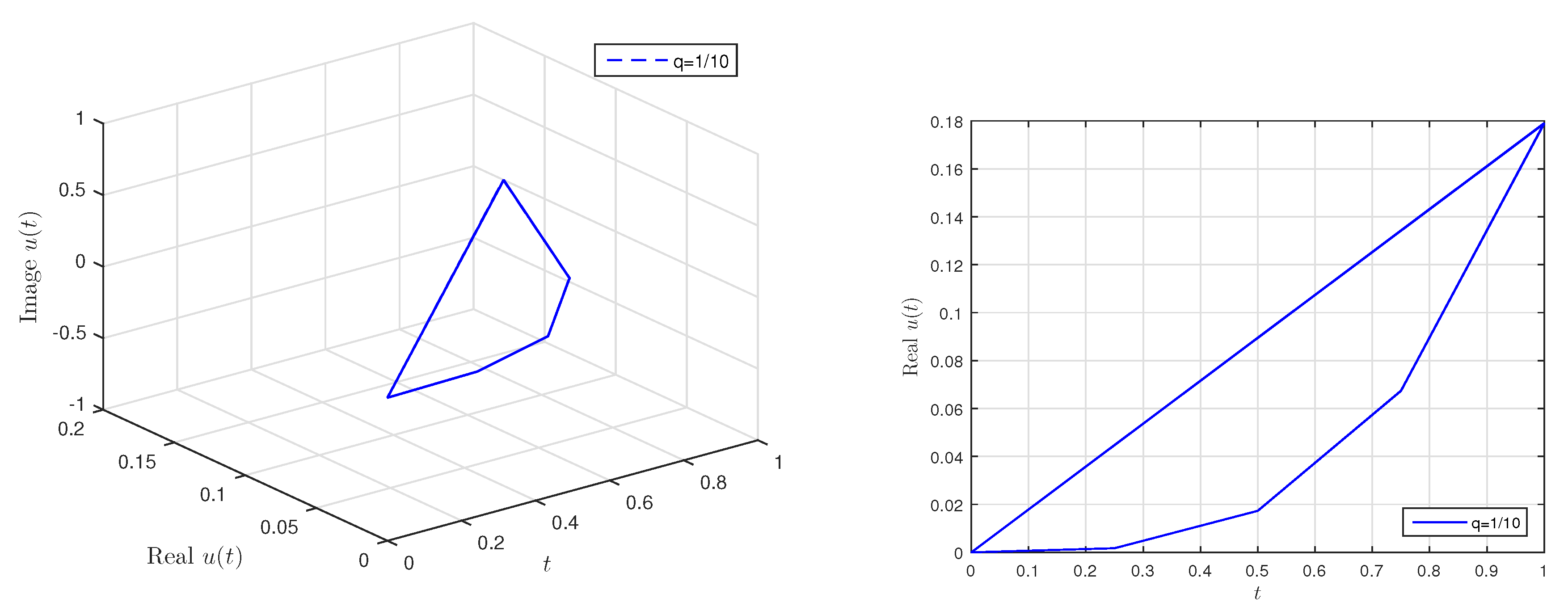
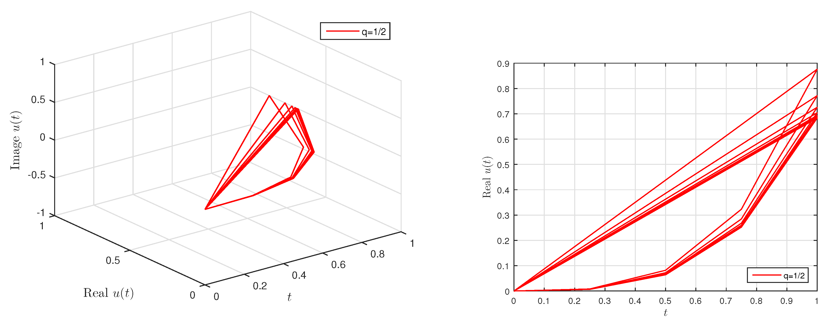
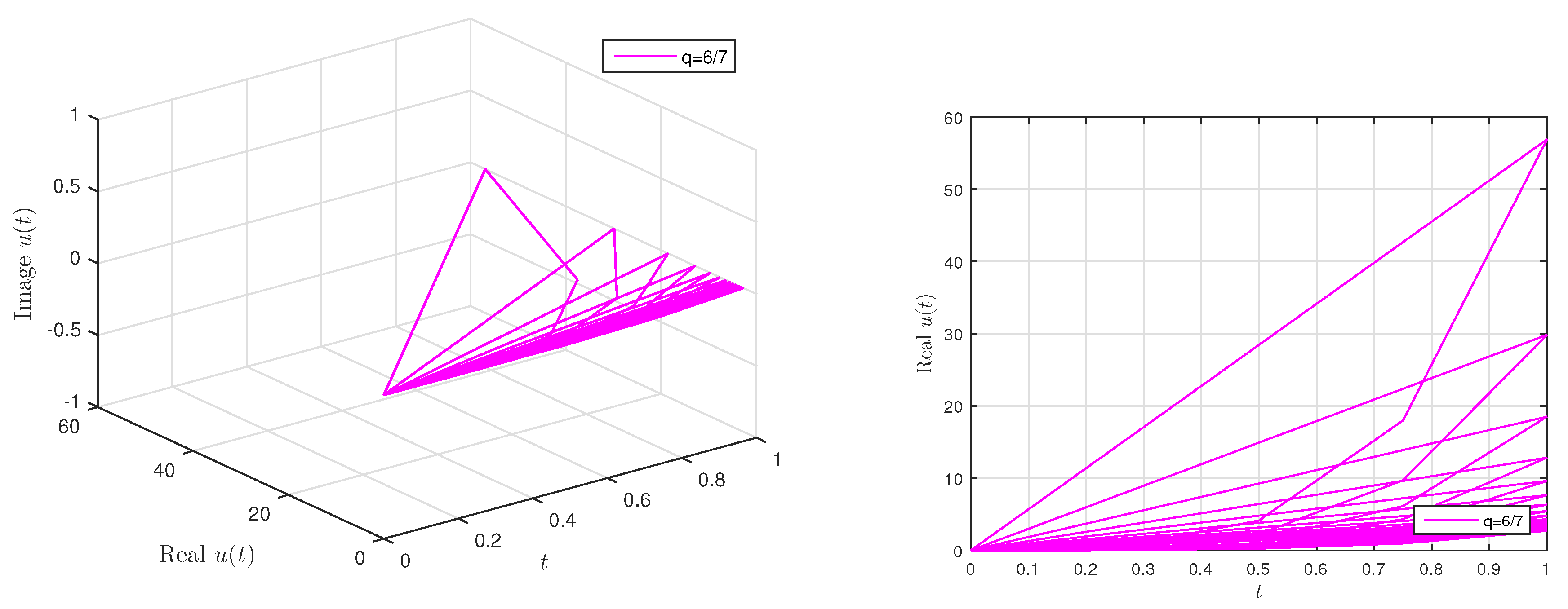
Example 1.

Consider the SFqDEq with the B.C:

$$\left\{\begin{array}{c}{}^c{\mathcal{D}}_q^{\frac{17}{5}}\left[u\right]\left(t\right)+\frac{|cost|}{t^2}\left[1+{\left(u\left(t\right)\right)}^3\right]=0,\hfill \\ \frac{15}{7}u\left(1\right)={\mathcal{I}}_q^{\frac{29}{7}}\left[u\right]\left(1\right),\hfill \\ u\left(0\right)=u^{″}\left(0\right)=u^{‴}\left(0\right)=\left(0\right)=0,\hfill \end{array}\right.$$

(4)

for all $t\in J=(0,1)$ and $q\in J$.

In Problem (1), define

$$\alpha =\frac{17}{5}\ge 3,n=\left[\frac{17}{5}\right]+1=4, c=\frac{15}{7}\ge 1,\gamma =\frac{29}{7}\in [1,\infty ).$$

Define the continuous map:

$$h(t,u\left(t\right))=\frac{|cost|}{t^2}\left[1+{\left(u\left(t\right)\right)}^3\right],$$

such that

$$\underset{t\to 0^{+}}{lim}h(t,.)=+\infty ,$$

that is, h is singular at $t=0$. In addition to, Table 1 shows that

$$2{\Gamma }_q\left(\gamma \right)\ge {\Gamma }_q\left(\alpha \right),$$

holds for each q.

Table 1. Numerical experiment for calculating ${\Gamma }_q\left(\alpha \right)$, ${\Gamma }_q\left(\gamma \right)$ in Example 1 for $q=\frac{1}{10},\frac{1}{2},\frac{8}{9}$.

n	$\mathit{q}=\frac{1}{10}$		$\mathit{q}=\frac{1}{2}$		$\mathit{q}=\frac{8}{9}$
	${\mathbf{\Gamma }}_{\mathit{q}}\left(\mathit{\alpha }\right)$	2${\mathbf{\Gamma }}_{\mathit{q}}\left(\mathit{\gamma }\right)$	${\mathbf{\Gamma }}_{\mathit{q}}\left(\mathit{\alpha }\right)$	2${\mathbf{\Gamma }}_{\mathit{q}}\left(\mathit{\gamma }\right)$	${\mathbf{\Gamma }}_{\mathit{q}}\left(\mathit{\alpha }\right)$	2${\mathbf{\Gamma }}_{\mathit{q}}\left(\mathit{\gamma }\right)$
1	$1.1479$	$2.4817$	$2.2951$	$7.2266$	$34.0843$	$265.2795$
2	$1.1467$	$2.4792$	$2.0569$	$6.414$	$21.5589$	$153.3424$
3	$1.1466$	$2.479$	$1.9515$	$6.056$	$15.299$	$101.2765$
4	$1.1466$	$2.479$	$1.9018$	$5.8876$	$11.7053$	$73.0841$
⋮	⋮	⋮	⋮	⋮	⋮	⋮
17	$1.1466$	$2.479$	$1.8539$	$5.7258$	$3.4748$	$16.2557$
18	$1.1466$	$2.479$	$1.8539$	$5.7258$	$3.3755$	$15.6765$
19	$1.1466$	$2.479$	$1.8539$	$5.7257$	$3.2907$	$15.1843$
20	$1.1466$	$2.479$	$1.8539$	$5.7257$	$3.2177$	$14.7638$
⋮	⋮	⋮	⋮	⋮	⋮	⋮
106	$1.1466$	$2.479$	$1.8539$	$5.7257$	$2.709$	$11.8963$
107	$1.1466$	$2.479$	$1.8539$	$5.7257$	$2.709$	$11.8963$
108	$1.1466$	$2.479$	$1.8539$	$5.7257$	$2.709$	$11.8963$
109	$1.1466$	$2.479$	$1.8539$	$5.7257$	$2.709$	$11.8962$
110	$1.1466$	$2.479$	$1.8539$	$5.7257$	$2.709$	$11.8962$

To numerically show our results, we consider the problem (2) as follows:

$$\begin{array}{cc}\hfill {\mathcal{D}}_q^{\frac{10}{3}}\left[u\right]\left(t\right)& +{\Gamma }_q\left(5\right)t^{-\frac{1}{9}}{\left|u\right|}^{\frac{1}{3}}+{\Gamma }_q\left(4\right)t^{-\frac{1}{9}}{\left|u^{\prime }\right|}^{\frac{2}{5}}\hfill \\ \hfill & +{\Gamma }_q\left(6\right)t^{-\frac{1}{9}}|{\mathcal{D}}_q^{\frac{4}{15}}{\left[u\right]\left(t\right)|}^{\frac{3}{4}}+{\Gamma }_q\left(3\right)t^{-\frac{1}{9}}{\left|v_u\right|}^{\frac{7}{9}}\hfill \\ \hfill & +\frac{1}{1+u^2\left(t\right)}+\frac{1}{1+{\left(u^{\prime }\right)}^2}+\frac{1}{1+{({\mathcal{D}}_q^{\frac{4}{15}}\left[u\right])}^2}+\frac{1}{1+{\left(v_u\right)}^2}\hfill \\ \hfill & \le {\mathcal{D}}_q^{\frac{10}{3}}\left[u\right]\left(t\right)+{\Gamma }_q\left(5\right)t^{-\frac{1}{9}}{\left|u\right|}^{\frac{1}{3}}+{\Gamma }_q\left(4\right)t^{-\frac{1}{9}}{\left|u^{\prime }\right|}^{\frac{2}{5}}\hfill \\ \hfill & +{\Gamma }_q\left(6\right)t^{-\frac{1}{9}}|{\mathcal{D}}_q^{\frac{4}{15}}{\left[u\right]\left(t\right)|}^{\frac{3}{4}}+{\Gamma }_q\left(3\right)t^{-\frac{1}{9}}{\left|v_u\right|}^{\frac{7}{9}}\hfill \\ \hfill & +{\left(u\left(t\right)\right)}^{-2}+{\left(u^{\prime }\right)}^{-2}+{({\mathcal{D}}_q^{\frac{4}{15}}\left[u\right])}^{-2}+{\left(v_u\right)}^{-2}=0.\hfill \end{array}$$

Thus,

$$\begin{array}{cc}\hfill {\mathcal{D}}_q^{\frac{10}{3}}\left[u\right]\left(t\right)& +{\Gamma }_q\left(5\right)t^{-\frac{1}{9}}{\left|u\right|}^{\frac{1}{3}}+{\Gamma }_q\left(4\right)t^{-\frac{1}{9}}{\left|u^{\prime }\right|}^{\frac{2}{5}}\hfill \\ \hfill & +{\Gamma }_q\left(6\right)t^{-\frac{1}{9}}|{\mathcal{D}}_q^{\frac{4}{15}}{\left[u\right]\left(t\right)|}^{\frac{3}{4}}+{\Gamma }_q\left(3\right)t^{-\frac{1}{9}}{\left|v_u\right|}^{\frac{7}{9}}\hfill \\ \hfill & +{\left(u\left(t\right)\right)}^{-2}+{\left(u^{\prime }\right)}^{-2}+{({\mathcal{D}}_q^{\frac{4}{15}}\left[u\right])}^{-2}+{\left(v_u\right)}^{-2}=0.\hfill \end{array}$$

(5)

Table 2 shows numerically the values of $x\left(t\right)$ in Equation (5). In addition, the curve of $x\left(t\right)$ w.r.t t in Figure 1, Figure 2 and Figure 3 for $q=\frac{1}{10}$, $\frac{1}{2}$, and $\frac{6}{7}$, respectively (Algorithm A1).

Table 2. Numerical experiment of Equation (5) in Example 1 for $q\in \left\{\frac{1}{10},\frac{1}{2},\frac{6}{7}\right\}$ and $n=1,\cdots 20$ (Algorithm A1).

n	$\mathit{q}=\frac{1}{10}$		$\mathit{q}=\frac{1}{2}$		$\mathit{q}=\frac{6}{7}$
	$\mathit{t}$	$\mathit{u}\left(\mathit{t}\right)$	$\mathit{t}$	$\mathit{u}\left(\mathit{t}\right)$	$\mathit{t}$	$\mathit{u}\left(\mathit{t}\right)$
1	$n=1$
1	0	0	0	0	0	0
1	$0.25$	$0.00172$	$0.25$	$0.00806$	$0.25$	$0.38812$
1	$0.5$	$0.01733$	$0.5$	$0.08187$	$0.5$	$4.1244$
1	$0.75$	$0.06744$	$0.75$	$0.32299$	$0.75$	$17.97576$
1	1	$0.17909$	1	$0.87607$	1	$56.89764$
2	$n=2$
2	0	0	0	0	0	0
2	$0.25$	$0.00171$	$0.25$	$0.0071$	$0.25$	$0.21494$
2	$0.5$	$0.01731$	$0.5$	$0.07216$	$0.5$	$2.26527$
2	$0.75$	$0.06737$	$0.75$	$0.2846$	$0.75$	$9.69401$
2	1	$0.17891$	1	$0.77148$	1	$29.82949$
⋮
20	$n=20$
	0	0	0	0	0	0
	$0.25$	$Inf$	$0.25$	$Inf$	$0.25$	$Inf$
	$0.5$	$Inf$	$0.5$	$Inf$	$0.5$	$Inf$
	$0.75$	$Inf$	$0.75$	$Inf$	$0.75$	$Inf$
	1	$Inf$	1	$Inf$	1	$Inf$
	$1.25$	$Inf$	$1.25$	$Inf$	$1.25$	$Inf$
	$1.5$	$Inf$	$1.5$	$Inf$	$1.5$	$Inf$
	$1.75$	$Inf$	$1.75$	$Inf$	$1.75$	$Inf$
	⋮	⋮	⋮	⋮	⋮	⋮

Figure 1. $u\left(t\right)$ with respect to t in Equation (5) in Example 1 for $q=\frac{1}{10}$ according to Table 2.

Figure 2. $u\left(t\right)$ with respect to t in Equation (5) in Example 1 for $q=\frac{1}{2}$ according to Table 2.

Figure 3. $u\left(t\right)$ with respect to t in Equation (5) in Example 1 for $\frac{6}{7}$ according to Table 2.

We can see that all conditions of Theorem 2 hold. Thus, the fixed point of Ω is a positive solution for problem (4).

Linear motion is the most basic of all motion. According to Newton’s first law of motion, objects that do not experience any net force will continue to move in a straight line with a constant velocity until they are subjected to a net force. In the next example, we consider an application to examine the validity of our theoretical results on the fractional order representation of the motion of a particle along a straight line.

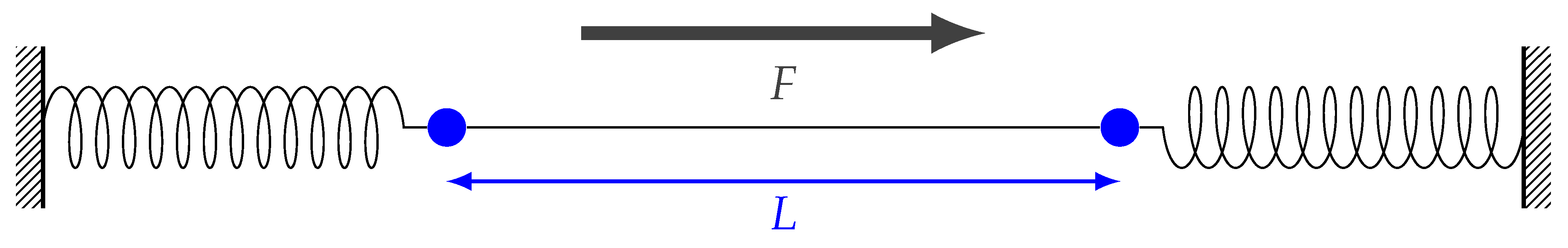
Example 2.

We consider a constrained motion of a particle along a straight line restrained by two linear springs with equal spring constants (stiffness coefficient) under an external force and fractional damping along the t-axis (Figure 4).

Figure 4. A particle along a straight line restrained by two linear springs with equal spring constants.

The springs, unless subjected to force, are assumed to have free length (unstretched length) and resist a change in length. The motion of the system along the t-axis is independent of the initial spring tension. The springs are anchored on the t-axis at $t=-1$ and $t=1$, and the vibration of the particle in this example is restricted to the t-axis only.

The vibration of the system is represented by a system of equations with the first equation having similar form of a simple harmonic oscillator, which cannot produce instability. Hence, the existence solution of the system depends on the following equation represented as the SFqDEq with the B.C:

$$\left\{\begin{array}{c}{}^c{\mathcal{D}}_q^{\frac{10}{3}}\left[u\right]\left(t\right)+\frac{1}{8}\left[2-2L-{\theta }^{2}L-{\theta }^{2}Lcost\right]u\left(t\right)=\nu sin\left(u\left(t\right)\right),\hfill \\ \frac{16}{9}u\left(1\right)={\mathcal{I}}_q^{\frac{23}{6}}\left[u\right]\left(1\right),\hfill \\ u\left(0\right)=u^{″}\left(0\right)=u^{‴}\left(0\right)=\left(0\right)=0,\hfill \end{array}\right.$$

(6)

for all $t\in J=(0,1)$, $q\in J$. Here, θ and ν are constants, and L is the unstretched length of the spring. In Problem (1),

$$\alpha =\frac{10}{3}\ge 3,n=\left[\frac{10}{3}\right]+1=4,\hspace{1em}c=\frac{16}{9}\ge 1,\gamma =\frac{23}{6}\in [1,\infty ).$$

Define the continuous map:

$$h(t,u\left(t\right))=\frac{1}{8}\left[2-2L-{\theta }^{2}L-{\theta }^{2}Lcost\right]u\left(t\right)-\nu sin\left(u\left(t\right)\right)$$

for $t\in (0,1)$, such that

$$\underset{t\to 0^{+}}{lim}h(t,.)=+\infty ,$$

that is, h is singular at $t=0$. Consider particular values of the parameters $L=1.5$ m, $\theta =0.5$. We consider particular values of the parameter $\nu =7.25$. Therefore, all conditions of Theorem 2 hold. Thus, the SFqDEq (6) has a solution.

5. Conclusions

The existence of solutions was successfully investigated for a system of m-singular sum fractional q-differential equations under some integral B.Cs in the sense of CpFqDr. The positive solutions’ existence was also studied with the help of a fixed point Arzelà–Ascoli theorem. Illustrative examples and numerical experiments were provided to validate our theoretical results.

References

1. Beyer, H.; Kempfle, S. Definition of physical consistent damping laws with fractional derivatives. Z. Angew. Math. Mech. 1995, 75, 623–635. [Google Scholar] [CrossRef]
2. He, J.H. Some applications of nonlinear fractional differential equations and their approximations. Sci. Technol. Soc. 1999, 15, 86–90. [Google Scholar]
3. He, J.H. Approximate analytic solution for seepage flow with fractional derivatives in porous media. Comput. Methods Appl. Mech. Eng. 1998, 167, 57–68. [Google Scholar] [CrossRef]
4. Caputo, M. Linear models of dissipation whose Q is almost frequency independent-II. Geophys. J. Int. 1967, 13, 529–539. [Google Scholar] [CrossRef]
5. Yan, J.P.; Li, C.P. On chaos synchronization of fractional differential equations. Chaos Solitons Fractals 2007, 32, 725–735. [Google Scholar] [CrossRef]
6. Sommacal, L.; Melchior, P.; Dossat, A.; Petit, J.; Cabelguen, J.M.; Oustaloup, A.; Ijspeert, A.J. Improvement of the muscle fractional multimodel for low-rate stimulation. Biomed. Signal Process. Control 2007, 2, 226–233. [Google Scholar] [CrossRef]
7. Rezapour, S.; Mojammadi, H.; Samei, M.E. SEIR epidemic model for COVID-19 transmission by Caputo derivative of fractional order. Adv. Differ. Equ. 2020, 2020, 490. [Google Scholar] [CrossRef] [PubMed]
8. Silva, M.F.; Machado, J.A.T.; Lopes, A.M. Fractional order control of a hexapod robot. Nonlinear Dyn. 2004, 38, 417–433. [Google Scholar] [CrossRef]
9. Mathieu, B.; Melchior, P.; Oustaloup, A.; Ceyral, C. Fractional differentiation for edge detection. Signal Process 2003, 83, 2421–2432. [Google Scholar] [CrossRef]
10. Diethelm, K.; Ford, N.J. Analysis of Fractional Differential Equations. J. Math. Anal. Appl. 2002, 265, 229–248. [Google Scholar] [CrossRef] [Green Version]
11. Mishra, S.K.; Samei, M.E.; Chakraborty, S.K.; Ram, B. On q-variant of Dai–Yuan conjugate gradient algorithm for unconstrained optimization problems. Nonlinear Dyn. 2021, 2021, 35. [Google Scholar] [CrossRef]
12. Ntouyas, S.K.; Samei, M.E. Existence and uniqueness of solutions for multi-term fractional q–integro-differential equations via quantum calculus. Adv. Differ. Equ. 2019, 2019, 475. [Google Scholar] [CrossRef]
13. Lakshmikantham, V.; Vatsala, A.S. Basic theory of fractional differential equations. Nonlinear Anal. Theory Methods Appl. 2008, 69, 2677–2682. [Google Scholar] [CrossRef]
14. Samei, M.E. Existence of solutions for a system of singular sum fractional q–differential equations via quantum calculus. Adv. Differ. Equ. 2020, 2020, 23. [Google Scholar] [CrossRef] [Green Version]
15. Matar, M.M.; Abbas, M.I.; Alzabut, J.; Kaabar, M.K.A.; Etemad, S.; Rezapour, S. Investigation of the p-Laplacian nonperiodic nonlinear boundary value problem via generalized Caputo fractional derivatives. Adv. Differ. Equ. 2021, 2021, 68. [Google Scholar] [CrossRef]
16. Jackson, F. q–difference equations. Am. J. Math. 1910, 32, 305–314. [Google Scholar] [CrossRef]
17. Adams, C. The general theory of a class of linear partial q–difference equations. Trans. Am. Math. Soc. 1924, 26, 283–312. [Google Scholar]
18. Adams, C. Note on the integro-q–difference equations. Trans. Am. Math. Soc. 1929, 31, 861–867. [Google Scholar]
19. Ahmad, B.; Nieto, J.J.; Alsaedi, A.; Al-Hutami, H. Existence of solutions for nonlinear fractional q–difference integral equations with two fractional orders and nonlocal four-point boundary conditions. J. Franklin Inst. 2014, 351, 2890–2909. [Google Scholar] [CrossRef]
20. Ahmad, B.; Ntouyas, S.; Purnaras, I. Existence results for nonlocal boundary value problems of nonlinear fractional q–difference equations. Adv. Differ. Equ. 2012, 2012, 140. [Google Scholar] [CrossRef] [Green Version]
21. Balkani, N.; Rezapour, S.; Haghi, R.H. Approximate solutions for a fractional q–integro-difference equation. J. Math. Ext. 2019, 13, 201–214. [Google Scholar]
22. Ferreira, R. Nontrivials solutions for fractional q–difference boundary value problems. Electron. J. Qual. Theory Differ. Equ. 2010, 70, 1–101. [Google Scholar] [CrossRef]
23. Samei, M.E.; Ranjbar, G.K.; Hedayati, V. Existence of solutions for equations and inclusions of multi-term fractional q–integro-differential with non-separated and initial boundary conditions. J. Inequalities Appl. 2019, 2019, 273. [Google Scholar] [CrossRef] [Green Version]
24. Zhao, Y.; Chen, H.; Zhang, Q. Existence results for fractional q–difference equations with nonlocal q–integral boundary conditions. Adv. Differ. Equ. 2013, 2013, 48. [Google Scholar] [CrossRef] [Green Version]
25. Agarwal, R.P.; Baleanu, D.; Hedayati, V.; Rezapour, S. Two fractional derivative inclusion problems via integral boundary condition. Appl. Math. Comput. 2015, 257, 205–212. [Google Scholar] [CrossRef]
26. Akbari Kojabad, E.; Rezapour, S. Approximate solutions of a sum-type fractional integro-differential equation by using Chebyshev and Legendre polynomials. Adv. Differ. Equ. 2017, 2017, 351. [Google Scholar] [CrossRef] [Green Version]
27. Liang, S.; Samei, M.E. New approach to solutions of a class of singular fractional q–differential problem via quantum calculus. Adv. Differ. Equ. 2020, 2020, 14. [Google Scholar] [CrossRef] [Green Version]
28. Aydogan, S.M.; Baleanu, D.; Mousalou, A.; Rezapour, S. On high order fractional integro-differential equations including the Caputo-Fabrizio derivative. Bound. Value Probl. 2018, 2018, 90. [Google Scholar] [CrossRef]
29. Baleanu, D.; Rezapour, S.; Etemad, S.; Alsaedi, A. On a time-fractional integro-differential equation via three-point boundary value conditions. Math. Probl. Eng. 2015, 2015, 12. [Google Scholar] [CrossRef]
30. He, C.Y. Almost Periodic Differential Equations; Higher Education Press: Beijing, China, 1992. (In Chinese) [Google Scholar]
31. Barbǎalat, I. Systems d’equations differential d’oscillations nonlinearies. Rev. Roumaine Math. Pure Appl. 1959, 4, 267–270. [Google Scholar]
32. Samei, M.E.; Hedayati, V.; Rezapour, S. Existence results for a fractional hybrid differential inclusion with Caputo-Hadamard type fractional derivative. Adv. Differ. Equ. 2019, 2019, 163. [Google Scholar] [CrossRef]
33. Annaby, M.; Mansour, Z. q–Fractional Calculus and Equations; Springer: Heidelberg, Germany; Cambridge, UK, 2012. [Google Scholar] [CrossRef]
34. Samko, S.; Kilbas, A.; Marichev, O. Fractional Integrals and Derivatives: Theory and Applications; Gordon and Breach Science Publishers: Lausanne, Switzerland; Philadelphia, PA, USA, 1993. [Google Scholar]
35. Krasnoselskii, M.A. Positive Solution of Operator Equation; Noordhoff: Groningen, The Netherlands, 1964. [Google Scholar]
36. Garrappa, R. Numerical Solution of Fractional Differential Equations: A Survey and a Software Tutorial. Mathematics 2018, 6, 16. [Google Scholar] [CrossRef] [Green Version]
Figure 1. u ( t ) with respect to t in Equation (5) in Example 1 for q = 1 10 according to Table 2.
Symmetry 13 01235 g001
Figure 2. u ( t ) with respect to t in Equation (5) in Example 1 for q = 1 2 according to Table 2.
Symmetry 13 01235 g002
Figure 3. u ( t ) with respect to t in Equation (5) in Example 1 for 6 7 according to Table 2.
Symmetry 13 01235 g003