A Generalized Rayleigh Family of Distributions Based on the Modified Slash Model

Abstract

Specifying a proper statistical model to represent asymmetric lifetime data with high kurtosis is an open problem. In this paper, the three-parameter, modified, slashed, generalized Rayleigh family of distributions is proposed. Its structural properties are studied: stochastic representation, probability density function, hazard rate function, moments and estimation of parameters via maximum likelihood methods. As merits of our proposal, we highlight as particular cases a plethora of lifetime models, such as Rayleigh, Maxwell, half-normal and chi-square, among others, which are able to accommodate heavy tails. A simulation study and applications to real data sets are included to illustrate the use of our results.

1. Introduction

Vodua [1] proposed a two-parameter distribution for the analysis of positive data, the well-known generalized Rayleigh distribution. This model overcomes the problems found in practice, which are related to a Rayleigh distribution and pointed out by authors, such as Siddiqui [2] and Hirano et al. [3]. Recall that a random variable (rv) X follows a generalized Rayleigh distribution, denoted as $X\sim \mathrm{GR}(\theta ,\alpha )$, if its probability density function (pdf) is given by the following:

$$f(x;\theta ,\alpha )=\frac{2{\theta }^{\alpha +1}}{\mathsf{\Gamma }(\alpha +1)}{x}^{2\alpha +1}{e}^{-\theta x^2},x>0,$$

(1)

where $\theta >0$ is a scale parameter, $\alpha >-1$ is a shape parameter and $\mathsf{\Gamma }\left(\alpha \right)={\int }_0^{\infty }{u}^{\alpha -1}{e}^{-u}du$ is the gamma function. The cumulative distribution function (cdf) of the GR distribution can be expressed as follows:

$$F(x;\theta ,\alpha )=\frac{\gamma (\alpha +1,\theta x^2)}{\mathsf{\Gamma }(\alpha +1)}=P(\alpha +1,\theta x^2),x>0,$$

(2)

where $\gamma (\alpha ,x)={\int }_0^x{u}^{\alpha -1}{e}^{-u}du$ is the incomplete gamma function and $P(\alpha +1,\theta x^2)$ denotes the regularized gamma function [4]. The moments of X are easily derived by using the results in [5] (Section 3.478). In fact, the rth distributional moment is as follows:

$${\mu }_r=E\left(X^r\right)=\frac{\mathsf{\Gamma }\left(\frac{r}{2}+\alpha +1\right)}{\mathsf{\Gamma }(\alpha +1){\theta }^{r/2}},r=1,2,3,...$$

(3)

Following the approach proposed in [6], lifetime models to accommodate outliers were proposed in [7]. We focus on the approach proposed in [8], where an extension of the generalized Rayleigh distribution called the slashed generalized Rayleigh distribution was introduced. This model has a kurtosis coefficient, which exhibits a wider range of values than the kurtosis coefficient in the GR distribution; therefore, it is appropriate to fit the data sets with outliers. Recall that a rv T follows a slashed generalized Rayleigh distribution, denoted as $T\sim \mathrm{SGR}(\theta ,\alpha ,q)$, if its stochastic representation is given by the following:

$$T=\frac{X}{U^{1/q}},q>0,$$

(4)

where $X\sim \mathrm{GR}(\theta ,\alpha )$ and $U\sim \mathrm{U}(0,1)$ are independent. The associated pdf is given by the following:

$$f_T(t;\theta ,\alpha ,q)=\frac{q{t}^{-(q+1)}}{\mathsf{\Gamma }(\alpha +1){\theta }^{q/2}}\mathsf{\Gamma }\left(\frac{2\alpha +q+2}{2}\right)F\left(\theta t^2,\frac{2\alpha +q+2}{2},1\right),t>0,$$

(5)

where $\theta >0$ is a scale parameter, $\alpha >-1$ is a shape parameter, $q>0$ is a kurtosis parameter and $F(x,\alpha ,\beta )={\int }_0^x\frac{{\beta }^{\alpha }}{\mathsf{\Gamma }\left(\alpha \right)}{t}^{\alpha -1}{e}^{-\beta t}dt$ is the cdf of a gamma distribution with shape parameter $\alpha >0$ and rate parameter $\beta >0$. If $\alpha =0$ and $\theta ={\left(2\sigma \right)}^{-1}$, the GR distribution reduces to the slashed-Rayleigh distribution. If $\alpha =-1/2$ and $\theta ={\left(2{\sigma }^2\right)}^{-1}$, the GR distribution reduces to slashed-half normal distribution [9].

In this work, we propose a modified version of the SGR distribution, given in (4), which can be used as an alternative model to the GR and SGR distributions.

We follow the idea proposed by [10], who introduced an extension of the normal distribution called modified slash (MS) distribution. A rv X follows a modified slash distribution, denoted as $X\sim \mathrm{MS}\left(q\right)$, if it can be written as follows:

$$X=\frac{Y}{W^{1/q}},q>0,$$

where $Y\sim \mathrm{N}(0,1)$ and $W\sim Exp\left(2\right)$ are independent. If $q\to \infty$, then the MS distribution converges in law to a normal distribution.

The paper is organized as follows. In Section 2 the stochastic representation, the pdf and ordinary moments of the proposed model are given. Section 3 is devoted to the family of distributions belonging to the generalized Rayleigh family of distributions based on the modified slash model. Among others, we can find here the modified slashed Rayleigh, half-normal, Maxwell and chi-square distributions. Recall that the unified treatment of a family of distributions is of interest in statistics; see, for instance, [11,12,13]. In Section 4, the estimation of parameters is discussed by considering the moments and maximum likelihood approaches. Similar to [14], their asymptotic normality is established. In addition, we carry out a simulation study to illustrate the performance of the estimators. In Section 5, two applications to real data sets are presented, where we illustrate that the proposed distribution may provide a better fit than the generalized Rayleigh and slashed generalized Rayleigh distributions. Finally, the main conclusions of this paper are given.

2. The New Model

In this section, some structural properties of the new model are given. These are the stochastic representation, pdf, hazard rate function and distributional moments.

2.1. Stochastic Representation

Definition 1.

A random variable T follows a modified slashed generalized Rayleigh distribution, denoted as $T\sim \mathrm{MSGR}(\theta ,\alpha ,q)$, if it can be expressed as follows:

$$T=\frac{X}{{\left(-\frac{1}{2}log\left(Z\right)\right)}^{1/q}},q>0,$$

(6)

where $X\sim \mathrm{GR}(\theta ,\alpha )$ and $Z\sim \mathrm{U}(0,1)$ are independent.

Remark 1.

• Let $T\sim \mathrm{MSGR}(\theta ,\alpha ,q)$. Then, T can be expressed as $T=X{Y}^{-1/q}$, where $X\sim \mathrm{GR}(\theta ,\alpha )$ and $Y\sim Exp\left(2\right)$ are independent.
• If $q=1$ then T follows a canonic modified slashed generalized Rayleigh (CMSGR) distribution, and we can write $T=-2X{log}^{-1}\left(Z\right)$, where $X\sim \mathrm{GR}(\theta ,\alpha )$ and $Z\sim \mathrm{U}(0,1)$ are independent. This is denoted as $T\sim \mathrm{CMSGR}(\theta ,\alpha )$.

The stochastic representation given in (6) can be used to generate values of $T\sim \mathrm{MSGR}(\theta ,\alpha ,q)$ by using the following algorithm:

• Generate $X\sim GR(\theta ,\alpha )$.
• Generate $Z\sim \mathrm{U}(0,1)$.
• Compute $T=X{\left(-\frac{1}{2}log\left(Z\right)\right)}^{-1/q}$.

2.2. Probability Density Function

To deal with the pdfs of generalized slash distributions, it is common to use hypergeometric functions as can be seen in [7,15,16]. In this subsection, we first introduce the special function, which is used in the expression of the pdf for the MSGR distribution, which is given in Proposition 1.

Definition 2.

For $\gamma >0$, $a>0$, $r>0$ and $s>0$, let us consider the following:

$$I(\gamma ,a,r,s)={\int }_0^{\infty }{x}^{\gamma -1}{e}^{-a{x}^r-sx}dx$$

(7)

where $I(·,·,·,·)$ is defined as in [17] (Equation 2.3.1.13).

Proposition 1.

Let $T\sim \mathrm{MSGR}(\theta ,\alpha ,q)$. Then, the pdf of T is given by the following:

$$f_T(t;\theta ,\alpha ,q)=\frac{2q{\theta }^{-\frac{q}{2}}}{\mathsf{\Gamma }(\alpha +1)t^{q+1}}I\left(\alpha +\frac{q}{2}+1,\frac{2}{{\theta }^{\frac{q}{2}}{t}^q},\frac{q}{2},1\right),t>0,$$

(8)

where $\theta >0$ is a scale parameter, $\alpha >-1$ is a shape parameter and $q>0$ is a kurtosis parameter.

Proof. 

From (6), and by applying the change of variable method, the pdf of T is given by the following:

$$\begin{array}{ccc}{f}_T(t;\theta ,\alpha ,q)& =& {\displaystyle \frac{4q{\theta }^{\alpha +1}}{\mathsf{\Gamma }(\alpha +1)}{t}^{2\alpha +1}{\int }_0^{\infty }{w}^{2\alpha +q+1}{e}^{-\theta {\left(tw\right)}^2-2w^q}dw}\hfill \\ & =& {\displaystyle \frac{2q{\theta }^{-\frac{q}{2}}}{\mathsf{\Gamma }(\alpha +1)t^{q+1}}{\int }_0^{\infty }{u}^{\alpha +\frac{q}{2}}{e}^{-u-2{\left(\frac{u}{\theta t^2}\right)}^{\frac{q}{2}}}du.}\hfill \end{array}$$

By considering $I(·,·,·,·)$, the integral introduced in Definition 2, (8) is obtained.  □

Corollary 1.

Let $T\sim \mathrm{MSGR}(\theta ,\alpha ,q)$. Then, the cdf of T is as follows:

$$F_T(t;\theta ,\alpha ,q)=\frac{2q}{\mathsf{\Gamma }(\alpha +1){\theta }^{\frac{q}{2}}}{\int }_0^t{u}^{-(q+1)}I\left(\alpha +\frac{q}{2}+1,\frac{2}{\theta u^q},\frac{q}{2},1\right)du$$

where $\mathsf{\Gamma }(·)$ is the gamma function and $I(·,·,·,·)$ was defined in (7).

As for the shape of the pdf in the MSGR model, we highlight that the pdf can be unimodal or monotonically decreasing. Plots of the pdf for certain values of the parameters are given in Figure 1. In Figure 1a,b, we can see that the parameter q is a kurtosis parameter since it mainly affects the right tail of the distribution. In Figure 1c, we can appreciate that the parameter $\theta$ is a scale-type parameter; the smaller the value of $\theta$, the more spread out the distribution [18]. Finally, in Figure 1d, we can see that the parameter $\alpha$ is a shape parameter.

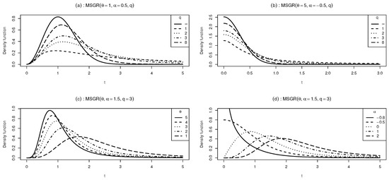
Figure 1. Plots of the MSGR pdf for certain values of its parameters.

2.3. Reliability Analysis

For non-negative rvs, it is of interest to know the reliability (or survival) function and the hazard rate function [19,20]. The reliability function, $R_T\left(t\right)=1-F_T\left(t\right)$, of a MSGR distribution is given by the following:

$$R_T(t;\theta ,\alpha ,q)=1-\frac{2q}{\mathsf{\Gamma }(\alpha +1){\theta }^{\frac{q}{2}}}{\int }_0^t{u}^{-(q+1)}I\left(u\right)du,$$

(9)

where $I\left(u\right)=I_{\theta ,\alpha ,q}\left(u\right)=I\left(\alpha +\frac{q}{2}+1,\frac{2}{{\theta }^{\frac{q}{2}}{u}^q},\frac{q}{2},1\right)$ is defined as in (7).

The hazard rate function, defined by $h_T\left(t\right)=\frac{f_T\left(t\right)}{R_T\left(t\right)}$, is given by the following:

$$h_T(t;\theta ,\alpha ,q)=\frac{t^{-(q+1)}I\left(t\right)}{{\displaystyle \frac{\mathsf{\Gamma }(\alpha +1){\theta }^{\frac{q}{2}}}{2q}-{\int }_0^t{u}^{-(q+1)}I\left(u\right)du}},$$

where $I\left(u\right)$ is as in (9) and $I\left(t\right)=I\left(\alpha +\frac{q}{2}+1,\frac{2}{{\theta }^{\frac{q}{2}}{t}^q},\frac{q}{2},1\right)$, defined in (7).

Figure 2 displays some plots of the hazard rate function of the MSGR distribution for different values of its parameters.

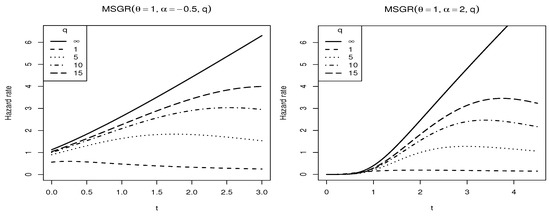
Figure 2. Plot of the hazard rate function for the MSGR distribution for different values of its parameters.

Applications of interest in engineering of the Rayleigh models can be seen in [21,22,23,24] among others. In these applications, it can be of interest to apply our proposal.

2.4. Moments

Next, we proceed to obtain the moments of the MGSR distribution. From these features, important characteristics of the model, such as the mean or expected value, variance, skewness and kurtosis coefficients are obtained. These results will also be the basis to apply the method of moments in Section 4.

Proposition 2.

Let $T\sim \mathrm{MSGR}(\theta ,\alpha ,q)$. Then, for $r=1,2,...$ and $q>r$ the rth distributional moment is given by the following:

$${\mu }_r=E\left(T^r\right)=\frac{2^{\frac{r}{q}}\mathsf{\Gamma }\left(\frac{q-r}{q}\right)\mathsf{\Gamma }\left(\frac{r}{2}+\alpha +1\right)}{\mathsf{\Gamma }(\alpha +1){\theta }^{\frac{r}{2}}}.$$

(10)

Proof. 

Using the stochastic representation given in Part 1 of Remark 1 and the independence of X and Y, it follows that

$${\mu }_r=E\left(T^r\right)=E\left({\left(\frac{X}{Y^{\frac{1}{q}}}\right)}^r\right)=E\left(X^r{Y}^{-\frac{r}{q}}\right)=E\left(X^r\right)E\left(Y^{-\frac{r}{q}}\right),$$

where $E\left(Y^{-\frac{r}{q}}\right)=2^{\frac{r}{q}}\mathsf{\Gamma }\left(\frac{q-r}{q}\right),q>r$ and $E\left(X^r\right)=\frac{\mathsf{\Gamma }\left(\frac{r}{2}+\alpha +1\right)}{\mathsf{\Gamma }(\alpha +1){\theta }^{\frac{r}{2}}}$ are distributional moments of the $Exp\left(2\right)$ and $\mathrm{GR}(\theta ,\alpha )$ distributions, respectively. □

Corollary 2.

Let $T\sim \mathrm{MSGR}(\theta ,\alpha ,q)$. Then, the mean and variance are, respectively, the following:

$$E\left(T\right)=\frac{2^{1/q}\mathsf{\Gamma }\left(\frac{q-1}{q}\right)\mathsf{\Gamma }\left(\alpha +3/2\right)}{\mathsf{\Gamma }(\alpha +1){\theta }^{1/2}},q>1,$$

and

$$Var\left(T\right)=\frac{2^{2/q}}{{\mathsf{\Gamma }}^2(\alpha +1)\theta }\left[\mathsf{\Gamma }(\alpha +1)\mathsf{\Gamma }(\alpha +2)\mathsf{\Gamma }\left(\frac{q-2}{q}\right)-{\mathsf{\Gamma }}^2\left(\alpha +3/2\right){\mathsf{\Gamma }}^2\left(\frac{q-1}{q}\right)\right],q>2.$$

Corollary 3.

Let $T\sim \mathrm{MSGR}(\sigma ,q)$. Then, the asymmetry (${\beta }_1$) and kurtosis (${\beta }_2$) coefficients are the following:

$$\begin{array}{ccc}{\beta }_1& =\hfill & {\displaystyle \frac{1}{A^{3/2}(\alpha ,q)}\left[{\mathsf{\Gamma }}^2(\alpha +1)\mathsf{\Gamma }\left(\alpha +5/2\right)\mathsf{\Gamma }\left(\frac{q-3}{q}\right)-3\mathsf{\Gamma }\left(\alpha +3/2\right)\mathsf{\Gamma }(\alpha +2)\mathsf{\Gamma }(\alpha +1)\right.}\hfill \\ & \hfill & {\displaystyle \times \left.\mathsf{\Gamma }\left(\frac{q-1}{q}\right)\mathsf{\Gamma }\left(\frac{q-2}{q}\right)+2{\mathsf{\Gamma }}^3\left(\alpha +3/2\right){\mathsf{\Gamma }}^3\left(\frac{q-1}{q}\right)\right],q>3,}\hfill \end{array}$$

and

$$\begin{array}{ccc}{\beta }_2& =\hfill & {\displaystyle \frac{1}{A^2(\alpha ,q)}\left[{\mathsf{\Gamma }}^3(\alpha +1)\mathsf{\Gamma }(\alpha +3)\mathsf{\Gamma }\left(\frac{q-4}{q}\right)-4\mathsf{\Gamma }\left(\alpha +3/2\right)\mathsf{\Gamma }\left(\alpha +5/2\right)\right.}\hfill \\ & \hfill & {\displaystyle \times {\mathsf{\Gamma }}^2(\alpha +1)\mathsf{\Gamma }\left(\frac{q-1}{q}\right)\mathsf{\Gamma }\left(\frac{q-3}{q}\right)+6{\mathsf{\Gamma }}^2\left(\alpha +3/2\right)\mathsf{\Gamma }(\alpha +1)\mathsf{\Gamma }(\alpha +2)}\hfill \\ & \hfill & {\displaystyle \times \left.{\mathsf{\Gamma }}^2\left(\frac{q-1}{q}\right)\mathsf{\Gamma }\left(\frac{q-2}{q}\right)-3{\mathsf{\Gamma }}^4\left(\alpha +3/2\right){\mathsf{\Gamma }}^4\left(\frac{q-1}{q}\right)\right],q>4,}\hfill \end{array}$$

where $A(\alpha ,q)=\mathsf{\Gamma }(\alpha +1)\mathsf{\Gamma }(\alpha +2)\mathsf{\Gamma }\left(\frac{q-2}{q}\right)-{\mathsf{\Gamma }}^2(\alpha +\frac{3}{2}){\mathsf{\Gamma }}^2\left(\frac{q-1}{q}\right)$.

Remark 2.

Notice that ${\beta }_1$ and ${\beta }_2$ do not depend on θ because it is a scale parameter. Furthermore, as $q\to \infty$ the ${\beta }_1$ and ${\beta }_2$ coefficients tend, respectively, to the following:

$${\beta }_{1_{GR}}=\frac{1}{A^{3/2}\left(\alpha \right)}\left[{\mathsf{\Gamma }}^2(\alpha +1)\mathsf{\Gamma }(\alpha +5/2)-3\mathsf{\Gamma }(\alpha +3/2)\mathsf{\Gamma }(\alpha +2)\mathsf{\Gamma }(\alpha +1)+2{\mathsf{\Gamma }}^3(\alpha +3/2)\right]$$

and

$$\begin{array}{ccc}{\beta }_{2_{GR}}& =\hfill & {\displaystyle \frac{1}{A^2\left(\alpha \right)}\left[{\mathsf{\Gamma }}^3(\alpha +1)\mathsf{\Gamma }(\alpha +3)-4\mathsf{\Gamma }(\alpha +3/2)\mathsf{\Gamma }(\alpha +5/2){\mathsf{\Gamma }}^2(\alpha +1)\right.}\hfill \\ & \hfill & +\left.6{\mathsf{\Gamma }}^2(\alpha +3/2)\mathsf{\Gamma }(\alpha +1)\mathsf{\Gamma }(\alpha +2)-3{\mathsf{\Gamma }}^4(\alpha +3/2)\right],\hfill \end{array}$$

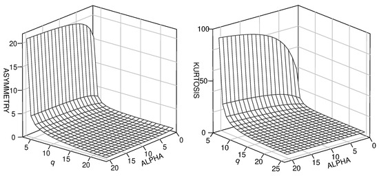
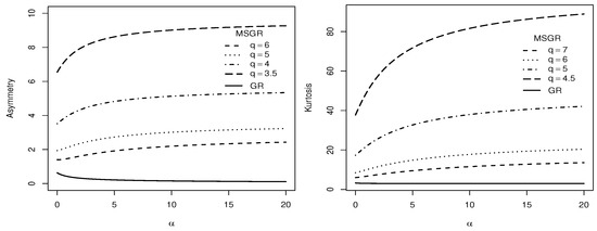
where $A\left(\alpha \right)=\mathsf{\Gamma }(\alpha +1)\mathsf{\Gamma }(\alpha +2)-{\mathsf{\Gamma }}^2(\alpha +3/2)$, which are the asymmetry and kurtosis coefficients of the GR distribution. Figure 3 depicts plots for the asymmetry and kurtosis coefficients of the MSGR model. In the figure, we observe that the highest values of asymmetry and kurtosis are associated with small values of parameter q and large values of parameter α. In addition, when comparing the asymmetry and kurtosis coefficients of the GR and MSGR distributions, we observe that q has a great impact on the increase in kurtosis, which is why we refer to q as a kurtosis parameter. This point is clearly observed in Figure 4.

Figure 3. Plots of the asymmetry and kurtosis coefficients for the MSGR model.

Figure 4. Plots of the asymmetry and kurtosis coefficients for the GR and MSGR models.

3. The MSGR Family of Distributions

In this section, we see that well-known models are associated with the MSGR family of distributions. Some of these results follow directly from (8) under certain reparameterizations, while other ones follow taking the limit when $q\to \infty$. Similar to the techniques used in [25], the limit distribution of (1) when $q\to \infty$ is obtained.

Lemma 1.

Let $T_q\sim MSGR(\theta ,\alpha ,q)$. Then, $T_q$ converges in distribution to $X\sim GR(\theta ,\alpha )$ when $q\to \infty$.

Proof. 

Let us consider the stochastic representation for $T_q$ given in Remark 1:

$$T_q=\frac{X}{Y^{1/q}}$$

where $X\sim GR(\theta ,\alpha )$ and $Y\sim Exp\left(2\right)$.

First, we prove the convergence in probability of $Y^{1/q}$ to a constant as $q\to \infty$. Since $Y\sim Exp\left(2\right)$ and $q>0$, we have the following:

$$\begin{array}{ccc}\hfill E[Y^{1/q}]& =& \frac{\mathsf{\Gamma }\left(1+\frac{1}{q}\right)}{2^{1/q}},\hfill \\ \hfill Var[Y^{1/q}]& =& \frac{\mathsf{\Gamma }\left(1+\frac{2}{q}\right)-{\mathsf{\Gamma }}^2\left(1+\frac{2}{q}\right)}{2^{2/q}}.\hfill \end{array}$$

By applying the Tchebychev inequality, we have the following:

$$P\left[\left|Y^{1/q}-E[Y^{1/q}]\right|>ϵ\right]\le \frac{Var[Y^{1/q}]}{{ϵ}^2}\forall ϵ>0,$$

(11)

and since $Var[Y^{1/q}]\to 0$ as $q\to \infty$ then

$$\{Y^{1/q}-E[Y^{1/q}]\}\stackrel{\mathcal{P}}{⟶}0.$$

Similarly, the sequence of real numbers behaves as follows:

$$E[Y^{1/q}]=\frac{\mathsf{\Gamma }\left(1+\frac{1}{q}\right)}{2^{1/q}}⟶1,q\to \infty .$$

Therefore,

$$Y^{1/q}=Y^{1/q}-E[Y^{1/q}]+E[Y^{1/q}]\stackrel{\mathcal{P}}{⟶}1\mathrm{as}q\to \infty .$$

By applying Slutsky’s theorem ([26] Corollary 2.3.2), we have the following:

$$T_q=\frac{X}{Y^{1/q}}\stackrel{d}{⟶}X\mathrm{as}q\to \infty$$

that is, $T_q$ converges in distribution to $X\sim GR(\theta ,\alpha )$ distribution. □

Next, we see that well-known models are particular cases of the $MSGR(\theta ,\alpha ,q)$ family of distributions. Specifically, for $\alpha =0$ and $\theta ={\left(2\sigma \right)}^{-1}$, the $MSGR$ model is reduced to the modified slashed Rayleigh distribution [27]. If $\alpha =-1/2$ and $\theta ={\left(2{\sigma }^2\right)}^{-1}$, then the $MSGR$ reduces to the modified slashed half-normal distribution [28]. For $\alpha =1/2$ and $\theta =\sigma /2$, we get the modified slashed Maxwell distribution. If $\alpha =\sigma /2-1$ and $\theta =1/2$, we obtain the modified slashed chi-square distribution. Taking the limit as $q\to \infty$ in previous models, the Rayleigh, half-normal [29], Maxwell [30] and chi-square distribution are obtained [31]. Details about these related models are given in the next corollaries. The relationships among these models are summarized in Figure 5.

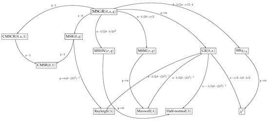
Figure 5. Relationships among distributions in the MSGR family.

Corollary 4

(Modified slashed Rayleigh model). Let $T\sim \mathrm{MSGR}(1/(2\sigma ),0,q)$. Then, T follows a modified slashed Rayleigh distribution, $\mathrm{MSR}(\sigma ,q)$, whose density function is given by the following:

$${\displaystyle f_T(t,\sigma ,q)=\frac{2^{\frac{q+2}{2}}q{\sigma }^{\frac{q}{2}}}{t^{q+1}}I\left(\frac{q}{2}+1,\frac{2^{\frac{q+2}{2}}{\sigma }^{\frac{q}{2}}}{t^q},\frac{q}{2},1\right),t>0,}$$

$\sigma >0$ is a scale parameter, $q>0$ is a kurtosis parameter [27].

As $q\to \infty$ then T converges in distribution to a Rayleigh distribution whose pdf is the following:

$$f_T\left(t\right)=\frac{t}{\sigma }{e}^{-\frac{t^2}{2\sigma }},t>0.$$

Corollary 5

(Modified slashed half-normal model). Let $T\sim \mathrm{MSGR}(1/2{\sigma }^2,1/2,q)$. Then, T follows a modified slashed half-normal distribution, $\mathrm{MSHN}(\sigma ,q)$, whose pdf is given by the following:

$$f_T(t;\sigma ,q)=\frac{2^{\frac{q+2}{2}}q{\sigma }^q}{\sqrt{\pi }{t}^{q+1}}I\left(\frac{q+1}{2},\frac{2^{\frac{q+2}{2}}{\sigma }^q}{t^q},\frac{q}{2},1\right),t>0,$$

where $\sigma >0$ is a scale parameter and $q>0$ is a kurtosis parameter [28].

As $q\to \infty$, T converges in distribution to a half-normal distribution whose pdf is the following:

$$f_T\left(t\right)=\frac{2}{\sigma }\varphi \left(\frac{t}{\sigma }\right),t>0,$$

where $\varphi (·)$ denotes the pdf of a $N(0,1)$ distribution.

Corollary 6

(Modified slashed Maxwell model). Let $T\sim \mathrm{MSGR}(\sigma /2,1/2,q)$. Then, T follows a modified slashed Maxwell distribution, $\mathrm{MSM}(\sigma ,q)$, whose pdf is given by the following:

$$f_T(t;\sigma ,q)={\left(\frac{2}{\sigma }\right)}^{\frac{q}{2}}\frac{4q}{\sqrt{\pi }{t}^{q+1}}I\left(\frac{q+3}{2},\frac{2^{\frac{q}{2}+1}}{{\sigma }^{\frac{q}{2}}{t}^q},\frac{q}{2},1\right),t>0,$$

where $\sigma >0$ is a scale parameter and $q>0$ is a kurtosis parameter.

As $q\to \infty$, T converges in distribution to a Maxwell distribution whose pdf is the following:

$$f_T\left(t\right)=\sqrt{\frac{2}{\pi }}{\sigma }^{3/2}{t}^2{e}^{-\frac{\sigma }{2}{t}^2},t>0.$$

Corollary 7

(Modified slashed chi-square model). Let $T\sim \mathrm{MSGR}(1/2,\sigma /2-1,q)$. Then, T follows a modified slashed chi-square distribution, MS${\chi }_{\sigma ,q}^2$, whose pdf is given by the following:

$$f_T(t;\sigma ,q)=\frac{2^{\frac{q}{2}+1}q}{\mathsf{\Gamma }\left(\frac{\sigma }{2}\right)t^{q+1}}I\left(\frac{\sigma +q}{2},\frac{2^{\frac{q}{2}+1}}{t^q},\frac{q}{2},1\right),t>0,$$

where $\sigma >0$ is a scale parameter and $q>0$ is a kurtosis parameter.

As $q\to \infty$, T converges in distribution to a gamma distribution with shape parameter $\sigma /2$ and rate parameter $1/2$ as follows:

$$f_T\left(t\right)=\frac{1}{2^{\sigma /2}\mathsf{\Gamma }(\sigma /2)}{t}^{\sigma /2-1}{e}^{-\frac{t}{2}},t>0.$$

If σ is a positive integer, then we have a chi-square distribution.

4. Parameter Estimation

In this section, we discuss moments and the maximum likelihood estimation for parameters $\theta$, $\alpha$ and q when sampling from the MSGR distribution. First, the moment method is introduced.

4.1. Method of Moments Estimators

Proposition 3.

Let $T_1,\cdots ,T_n$ be a random sample of size n from the $T\sim \mathrm{MSGR}(\theta ,\alpha ,q)$ distribution. Then, the method of moments estimates of $(\theta ,\alpha ,q)$ for $q>3$ are given by the following:

$$\begin{array}{ccc}\hfill \widehat{\theta }& =& \frac{2^{2/\widehat{q}}{\mathsf{\Gamma }}^2\left(\frac{\widehat{q}-1}{\widehat{q}}\right){\mathsf{\Gamma }}^2\left(\widehat{\alpha }+\frac{3}{2}\right)}{{\mathsf{\Gamma }}^2(\widehat{\alpha }+1){\overline{T}}^2},\hfill \end{array}$$

(12)

$$\begin{array}{ccc}\hfill \widehat{\alpha }& =& \frac{\frac{3}{2}{d}_2-d_1}{d_1-d_2},\hfill \end{array}$$

(13)

$$\begin{array}{ccc}\hfill \frac{{\overline{T}}^2}{\overline{T^2}}& =& \frac{{\mathsf{\Gamma }}^2\left(\frac{\widehat{q}-1}{\widehat{q}}\right){\mathsf{\Gamma }}^2\left(\frac{\frac{3}{2}{d}_2-d_1}{d_1-d_2}+\frac{3}{2}\right)}{\mathsf{\Gamma }\left(\frac{\widehat{q}-2}{\widehat{q}}\right)\mathsf{\Gamma }\left(\frac{\frac{3}{2}{d}_2-d_1}{d_1-d_2}+2\right)\mathsf{\Gamma }\left(\frac{\frac{3}{2}{d}_2-d_1}{d_1-d_2}+1\right)},\hfill \end{array}$$

(14)

with $d_1=\frac{{\overline{T}}^2}{\overline{T^2}}\mathsf{\Gamma }\left(\frac{q-1}{q}\right)\mathsf{\Gamma }\left(\frac{q-2}{q}\right)$, $d_2=\frac{{\overline{T}}^3}{\overline{T^3}}\mathsf{\Gamma }\left(\frac{q-3}{q}\right)$ and ${\overline{T}}_k=(1/n){\sum }_{i=1}^n{T}_i^k$, $k=1,2,3$.

Proof. 

First, from Proposition 2 and taking into account the first three equations in the moments method, we have the following:

$$\overline{T}=\frac{2^{1/q}\mathsf{\Gamma }\left(\frac{q-1}{q}\right)\mathsf{\Gamma }(\alpha +3/2)}{\mathsf{\Gamma }(\alpha +1){\theta }^{1/2}},\overline{T^2}=\frac{2^{2/q}\mathsf{\Gamma }\left(\frac{q-2}{q}\right)\mathsf{\Gamma }(\alpha +2)}{\mathsf{\Gamma }(\alpha +1)\theta },\overline{T^3}=\frac{2^{3/q}\mathsf{\Gamma }\left(\frac{q-3}{q}\right)\mathsf{\Gamma }(\alpha +5/2)}{\mathsf{\Gamma }(\alpha +1){\theta }^{3/2}}.$$

(15)

Now, consider the above equations for the following:

• Solving for $\theta$, the second of the above equations, the result in (12) is obtained.
• Solving for $\theta$, the first two of the above equations, and matching the resulting expressions, we obtain the following:

  $$\frac{{\mathsf{\Gamma }}^2\left(\frac{q-1}{q}\right){\mathsf{\Gamma }}^2(\alpha +3/2)}{\mathsf{\Gamma }(\alpha +1)}=\frac{{\overline{T}}^2}{\overline{T^2}}\mathsf{\Gamma }\left(\frac{q-2}{q}\right)\mathsf{\Gamma }(\alpha +2),$$

  (16)

  and solving the first and third of the equations in (15), we have the following:

  $$\frac{{\mathsf{\Gamma }}^2\left(\frac{q-1}{q}\right){\mathsf{\Gamma }}^2(\alpha +3/2)}{\mathsf{\Gamma }(\alpha +1)}=\frac{{\overline{T}}^3}{\overline{T^3}}{\mathsf{\Gamma }}^{-1}\left(\frac{q-1}{q}\right)\mathsf{\Gamma }\left(\frac{q-3}{q}\right)(\alpha +3/2)\mathsf{\Gamma }(\alpha +1)$$

  (17)
  Equating (16) and (17), and considering an appropriate algebraic manipulation, the result in (13) is obtained.
• Finally, substituting (13) in (16), by a straightforward calculation, the result in (14) is obtained.

□

4.2. Maximum Likelihood Estimation

Now, the maximum likelihood (ML) estimates of parameters in the MSGR distribution, based on a random sample of size n, are obtained. Given an observed sample $t_1,\dots ,t_n$ from the $\mathrm{MSGR}(\theta ,\alpha ,q)$ distribution, the log-likelihood function for the parameters $\theta$, $\alpha$ and q, given $t=(t_1,\dots ,t_n)$, can be written as the following:

$$logL(\vartheta ;t_i)=c(\theta ,\alpha ,q)-(q+1){\displaystyle \sum _{i=1}^n}log\left(t_i\right)+{\displaystyle \sum _{i=1}^n}logI\left(\alpha +\frac{q}{2}+1,\frac{2}{{\theta }^{\frac{q}{2}}{t}_i^q},\frac{q}{2},1\right),$$

(18)

where $c(\theta ,\alpha ,q)=nlog\left(2\right)+nlog\left(q\right)-\frac{nq}{2}log\left(\theta \right)-nlog\mathsf{\Gamma }(\alpha +1)$ and $\vartheta =(\theta ,\alpha ,q)$. The maximum likelihood equations are given by the following:

$${\displaystyle \begin{array}{r}-\frac{nq}{2\theta }+{\displaystyle \sum _{i=1}^n}\frac{I_1\left(t_i\right)}{I\left(t_i\right)}=0,\end{array}}$$

(19)

$${\displaystyle \begin{array}{r}-n\mathsf{\Psi }(\alpha +1)+{\displaystyle \sum _{i=1}^n}\frac{I_2\left(t_i\right)}{I\left(t_i\right)}=0,\end{array}}$$

(20)

$${\displaystyle \begin{array}{r}\frac{n}{q}-\frac{n}{2}log\left(\theta \right)-{\displaystyle \sum _{i=1}^n}log\left(t_i\right)+{\displaystyle \sum _{i=1}^n}\frac{I_3\left(t_i\right)}{I\left(t_i\right)}=0,\end{array}}$$

(21)

where $\mathsf{\Psi }(·)$ is the digamma function,

$$\begin{array}{c}I\left(t_i\right)=I\left(\alpha +\frac{q}{2}+1,\frac{2}{{\theta }^{\frac{q}{2}}{t}_i^q},\frac{q}{2},1\right),I_1\left(t_i\right)=\frac{\partial }{\partial \theta }I\left(\alpha +\frac{q}{2}+1,\frac{2}{{\theta }^{\frac{q}{2}}{t}_i^q},\frac{q}{2},1\right),\hfill \\ I_2\left(t_i\right)=\frac{\partial }{\partial \alpha }I\left(\alpha +\frac{q}{2}+1,\frac{2}{{\theta }^{\frac{q}{2}}{t}_i^q},\frac{q}{2},1\right)\mathrm{and}{I}_3\left(t_i\right)=\frac{\partial }{\partial q}I\left(\alpha +\frac{q}{2}+1,\frac{2}{{\theta }^{\frac{q}{2}}{t}_i^q},\frac{q}{2},1\right).\hfill \end{array}$$

Solutions for Equations (19)–(21) can be obtained by using numerical procedures, such as the Newton–Raphson procedure. The observed information matrix for the parameters $\theta$, $\alpha$ and q is given by the following:

$${\displaystyle {\mathbf{I}}_n(\theta ,\alpha ,q)=\left(\begin{array}{ccc}\frac{nq}{2{\theta }^2}+G_{\theta ,1}\left(t_i\right)& G_{\alpha ,1}\left(t_i\right)& -\frac{n}{2\theta }+G_{q,1}\left(t_i\right)\\ G_{\theta ,2}\left(t_i\right)& -n{\mathsf{\Psi }}_1(\alpha +1)+G_{\alpha ,2}\left(t_i\right)& G_{q,2}\left(t_i\right)\\ -\frac{n}{2\theta }+G_{\theta ,3}\left(t_i\right)& G_{\alpha ,3}\left(t_i\right)& -\frac{n}{q^2}+G_{q,3}\left(t_i\right)\end{array}\right)}$$

where $G_{\nu ,k}\left(t_i\right)={\sum }_{i=1}^n\frac{d}{d\nu }\frac{I_k\left(t_i\right)}{I\left(t_i\right)}$, $\nu =\theta ,\alpha ,q$, and ${\mathsf{\Psi }}_1$ is the trigamma function, with $I_k\left(t_i\right)$, $k=1,2,3$, given in Equations (19)–(21), respectively.

Asymptotic confidence intervals and hypothesis tests for a given parameter in the model can be obtained by using the observed information matrix ${\mathbf{I}}_n\left(\gamma \right)$, with $\gamma =(\theta ,\alpha ,q)$. They can be deduced by assuming that the maximum likelihood estimator has approximately a $N_3(\gamma ,K_{\gamma }^{-1})$ distribution, where $K_{\gamma }={lim}_{n\to \infty }{n}^{-1}{\mathbf{I}}_n\left(\gamma \right)$. In practice, the matrix ${\mathbf{I}}_n\left(\gamma \right)$, evaluated at $\widehat{\gamma }$ is used since there is no closed-form expression for the expected information matrix $K_{\gamma }$ for $\gamma$.

4.3. Maximum Likelihood Estimation via the EM Algorithm

The EM algorithm (Dempster et al. [32]) is a useful method for ML estimation in the presence of latent variables. To carry out the estimation process, we introduce latent variables $W_1,...,W_n$ through the following hierarchical representation of the MSGR model:

$$T_i|W_i=w_i\sim GR(w_i^2\theta ,\alpha )$$

$$W_i\sim Wei(q,1/2)$$

where $Wei(q,1/2)$ denotes a Weibull distribution. The joint pdf of $(T_i,W_i)$ is as follows:

$$f(t_i,w_i)=\frac{2{\left(w_i^2\theta \right)}^{\alpha +1}}{\mathsf{\Gamma }(\alpha +1)}{t}_i^{2\alpha +1}exp\{-w_i^2\theta t_i^2\}2q{w}_i^{q-1}exp\{-2w_i^q\}.$$

The full log-likelihood function is the following:

$$\begin{array}{ccc}\hfill l_c\left(\vartheta \right)& =& 2(\alpha +1){\displaystyle \sum _{i=1}^n}log{w}_i+n(\alpha +1)log\theta +(2\alpha +1){\displaystyle \sum _{i=1}^n}log{t}_i-nlog\mathsf{\Gamma }(\alpha +1)\hfill \\ & -& \theta {\displaystyle \sum _{i=1}^n}{w}_i^2{t}_i^2+nlog\left(q\right)+(q-1){\displaystyle \sum _{i=1}^n}log{w}_i-2{\displaystyle \sum _{i=1}^n}{w}_i^q+constant\hfill \end{array}$$

with $\vartheta =(\theta ,\alpha ,q)$. To apply the EM algorithm, it is necessary to obtain $\widehat{log\left(w_i\right)}=E(log\left(w_i\right)|T_i=t_i,\vartheta =\widehat{\vartheta })$ and $\widehat{w_i^2}=E(w_i^2|T_i=t_i,\vartheta =\widehat{\vartheta })$.

Finally, the k-th step of the algorithm is as follows:

Step E: Using ${\widehat{\theta }}^{(k-1)}$, ${\widehat{\alpha }}^{(k-1)}$ and ${\widehat{q}}^{(k-1)}$, calculate $\widehat{log{w}_i^{\left(k\right)}}$ and $\widehat{w_i^{2\left(k\right)}}$, $i=1,\dots ,n.$

Step ECME I: Using ${\widehat{\alpha }}^{(k-1)}$, update $\theta$ as follows:

$${\widehat{\theta }}^{\left(k\right)}=\frac{n({\widehat{\alpha }}^{(k-1)}+1)}{{\sum }_{i=1}^n{\widehat{w_i}}^{2\left(k\right)}{t}_i^2}.$$

Step ECME II: Update $\alpha$ as follows:

$${\widehat{\alpha }}^{\left(k\right)}={\mathsf{\Psi }}^{-1}\left(\frac{2{\sum }_{i=1}^n\left(\widehat{log{w}_i^{\left(k\right)}}+log{t}_i\right)+nlog{\widehat{\theta }}^{\left(k\right)}}{n}\right)-1,$$

where ${\mathsf{\Psi }}^{-1}(·)$ denotes the inverse of the digamma function.

Step ECME III: Fix $\alpha ={\alpha }^{\left(k\right)}$ and $\theta ={\theta }^{\left(k\right)}$, update q using the log-likelihood observed as follows:

$$q^{\left(k\right)}=argma{x}_{q>0}l({\alpha }^{\left(k\right)},{\theta }^{\left(k\right)},q).$$

This procedure is repeated until a suitable convergence rule is satisfied. Useful starting values are required to start the recursion.

4.4. Simulation Study

To check the good behavior of ML estimators in the MSGR model, a simulation study is carried out by using R software [33]. In this study, 1000 samples of sample size $n=100$, 200 and 300 were generated from the MSGR model. The aim of this simulation is to study the performance of the ML estimators for the parameters using the proposed procedure.

For each generated sample, the ML estimates for each parameter were computed numerically. The mean value and standard deviation (SD) of the estimates for the parameters $(\theta ,\alpha ,q)$ are given as summaries in Table 1. It can be seen there that the ML estimates are quite stable and close to the real values for the sample sizes under consideration. As expected, the bias and standard deviation of our estimates decrease as the sample size n increases.

Table 1. Empirical means and SD for the ML estimators of $\theta$, $\alpha$ and q.

$\mathit{\theta }$		$\mathit{\alpha }$	q	$\widehat{\mathit{\theta }}$ (SD)	$\widehat{\mathit{\alpha }}$ (SD)	$\widehat{\mathit{q}}$ (SD)
$n=50$
	1	−0.5	2	1.249 (0.897)	−0.459 (0.233)	2.586 (1.101)
	1	−0.5	3	1.183 (0.674)	−0.435 (0.171)	3.442 (1.615)
	1	−0.5	4	1.117 (0.543)	−0.468 (0.132)	4.275 (1.568)
	1	−0.5	3	1.172 (0.830)	0.597 (0.517)	3.137 (1.471)
	1	0.0	3	1.182 (0.842)	0.099 (0.274)	3.116 (0.977)
	1	3.0	3	1.245 (0.897)	3.208 (1.811)	3.258 (0.793)
	1	2.0	3	1.296 (1.098)	2.269 (1.607)	3.369 (1.816)
	2	2.0	3	2.433 (1.659)	2.240 (1.356)	3.197 (0.918)
	3	2.0	3	3.212 (2.365)	2.084 (1.206)	3.247 (0.861)
$n=100$
	1	−0.5	2	1.223 (0.888)	−0.472 (0.105)	2.151 (0.662)
	1	−0.5	3	1.137 (0.551)	−0.478 (0.082)	3.225 (1.021)
	1	−0.5	4	1.093 (0.497)	−0.481 (0.074)	4.095 (1.261)
	1	−0.5	3	1.096 (0.498)	0.591 (0.401)	3.135 (0.666)
	1	0.0	3	1.131 (0.539)	0.057 (0.252)	3.064 (0.672)
	1	3.0	3	1.239 (0.821)	2.828 (0.998)	3.138 (0.555)
	1	2.0	3	1.276 (0.821)	2.250 (1.115)	3.117 (0.566)
	2	2.0	3	2.217 (0.957)	2.237 (0.990)	3.107 (0.598)
	3	2.0	3	2.848 (0.923)	2.068 (0.841)	3.135 (0.617)
$n=200$
	1	−0.5	2	1.127 (0.562)	−0.475 (0.096)	2.075 (0.451)
	1	−0.5	3	1.072 (0.467)	−0.497 (0.062)	3.018 (0.736)
	1	−0.5	4	1.016 (0.387)	−0.501 (0.055)	4.051 (0.742)
	1	−0.5	3	1.044 (0.388)	0.504 (0.301)	3.070 (0.598)
	1	0.0	3	1.010 (0.376)	0.010 (0.168)	3.046 (0.585)
	1	3.0	3	0.994 (0.443)	2.944 (0.890)	3.080 (0.481)
	1	2.0	3	1.144 (0.643)	2.156 (0.514)	3.078 (0.462)
	2	2.0	3	2.036 (0.792)	2.015 (0.764)	3.081 (0.498)
	3	2.0	3	3.087 (0.746)	2.061 (0.680)	3.092 (0.511)

5. Illustrations

In this section, two applications based on real data sets are given. The aim is to compare the fit provided by the MSGR, SGR and GR models. As one of the referees points out, a validation of the virtues of our proposal would require a large number of successful applications. So, the reader must be cautious. It can be said that our aim is to illustrate the use of these models.

5.1. Active Repair Time Data

The first illustration consists of $n=46$ lifetime data (in hours) for an airborne communication transceiver. This data set was previously studied by [34]. Table 2 presents the statistics summaries for these data. These are the sample mean, sample variance ($s^2$), $b_1$ and $b_2$, which denote the sample asymmetry and kurtosis coefficients, respectively. We highlight the fact that the sample kurtosis coefficient $b_2$ is higher than expected for a GR distribution. Therefore, it makes sense to fit a MSGR model.

Table 2. Descriptive statistics for the active repair time data.

n	$\overline{\mathit{X}}$	${\mathit{s}}^2$	${\mathit{b}}_1$	${\mathit{b}}_2$
46	3.606	24.445	2.794	11.294

First, the moment estimators under the MSGR model were computed. We obtained the following estimates: ${\widehat{\theta }}_M=0.011$, ${\widehat{\alpha }}_M=-0.803$ and ${\widehat{q}}_M=4.638$. Using the method of moment estimates as the initial values, the maximum likelihood estimates were computed and are presented in Table 3; their standard errors (s.e) are given in parenthesis. For every model, we also give the estimated log-likelihood value.

Table 3. Maximum likelihood estimates, log-likelihood estimated value and respective AIC, BIC, KS statistics for GR, SGR and MSGR models.

Parmeters	GR (s.e)	SGR (s.e)	MSGR (s.e)
$\widehat{\theta }$	0.008 (0.002)	2.121 (2.316)	2.772 (0.132)
$\widehat{\alpha }$	−0.696 (0.049)	0.241 (0.640)	0.731 (0.091)
$\widehat{q}$	-	0.859 (0.202)	1.182 (0.080)
Log-likelihood	111.041	101.888	100.292
AIC	226.083	209.776	206.585
BIC	229.740	215.262	212.071
KS	0.173	0.152	0.108

In order to compare distributions with different numbers of parameters, the Akaike information criterion (AIC) [35] and Bayesian information criterion (BIC) [36] were computed. Recall that $AIC=2k-2log\mathrm{lik}$ and $BIC=klogn-2log\mathrm{lik}$, where k is the number of parameters in the model, n is the sample size and $log\mathrm{lik}$ is the maximized value of the log-likelihood function. The Kolmogorov–Smirnov statistic (KS) is considered. In Table 3, the corresponding AIC, BIC and KS statistics are reported for each fitted model. Note that the AIC, BIC and KS statistics values show that the better fit is provided by the MSGR model. Figure 6 depicts the histogram of this data set, including the estimated densities under the MSGR, SGR, and GR models. Finally, the Q–Q plots are given in Figure 7, where we can again see that the MSGR model fits better than the GR and SGR models.

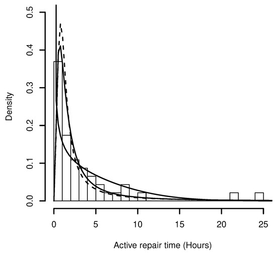
Figure 6. Fitted models by ML method for active repair time data set: MSGR (solid line), SGR (dashed line), GR (dotted line).

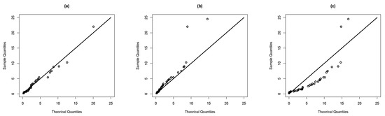
Figure 7. QQ-plots: (a) MSGR model, (b) SGR model, (c) GR model.

5.2. Remission Time Data

The second data set corresponds to the remission times (in months) of a random sample of $n=128$ bladder cancer patients. This data set can be found in [37]. Table 4 presents the statistics summaries for this data set. Notice that sample kurtosis $b_2$ is quite high.

Table 4. Descriptive statistics of the remission time data.

n	$\overline{\mathit{X}}$	${\mathit{s}}^2$	${\mathit{b}}_1$	${\mathit{b}}_2$
128	9.365	110.425	3.286	18.483

Computing initially the moment estimators under the MSGR model we have the following estimates: ${\widehat{\theta }}_M=0.003$, ${\widehat{\alpha }}_M=-0.681$ and ${\widehat{q}}_M=4.071$. Using the moment estimators as initial values, the maximum likelihood estimates are computed and presented in Table 5 with the standard errors in parenthesis. Table 5 also reports the log-likelihood estimated value and the corresponding AIC, BIC and KS statistic for each fitted model. Figure 8 depicts the histogram of this data set, including the estimated densities under the MSGR, SGR, GR models. Finally, from the Q–Q plots in Figure 9 we can observe that the MSGR model fits better than the GR and SGR models.

Table 5. Maximum likelihood estimates, log-likelihood estimated value and respective AIC, BIC, KS statistics for GR, SGR and MSGR models.

Parameters	GR (s.e)	SGR (s.e)	MSGR (s.e)
$\widehat{\theta }$	0.002 (0.0002)	0.019 (0.007)	0.023 (0.009)
$\widehat{\alpha }$	−0.610 (0.035)	−0.390 (0.086)	−0.355 (0.100)
$\widehat{q}$	-	1.839 (0.381)	2.213 (0.402)
Log-likelihood	−426.824	−410.183	−409.695
AIC	859.648	826.366	825.391
BIC	868.204	834.922	833.947
KS	0.156	0.070	0.062

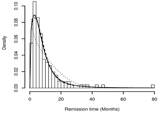
Figure 8. Fitted models by ML method for remission time data set: MSGR (solid line), SGR (dashed line), GR (dotted line).

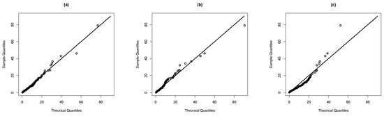
Figure 9. QQ-plots: (a) MSGR model, (b) SGR model, (c) GR model.

6. Concluding Remarks

In this article, a new generalization of the GR distribution, which is able to model positive data with high kurtosis, is introduced. The proposed distribution can be written as the ratio of two independent random variables. These are a GR distribution and a power of the exponential distribution. We derived some special cases that can be seen as two-parameter extensions of the Rayleigh, half normal, Maxwell and chi square distributions. The parameters were estimated by using moments and maximum likelihood methods. The method of moments estimates were used to start the maximum likelihood estimation through the Newton–Raphson procedure. The asymmetry and kurtosis coefficients were also obtained. The study of these coefficients illustrates the fact that the MSGR model can be used to describe positive right-skewed data with high kurtosis. Finally, the MSGR model was fitted to two real data sets. In both applications, the MSGR distribution presented a better fit than the GR and SGR models, which shows the potential applicability of our proposal. To conclude, we point out that these models can be used not only in reliability studies, but also in the fields of economics, for instance, to describe financial data, where models with heavy tails are very interesting.

References

- Vodă, V.G. Inferential procedures on a generalized Rayleigh variate I. Apl. Mat. 1976, 21, 395–412. [Google Scholar]
- Siddiqui, M.M. Some problems connected with Rayleigh distributions. J. Res. Natl. Bur. Stand. Sect. D Radio Propag. 1962, 66, 167–174. [Google Scholar] [CrossRef]
- Hirano, K. Rayleigh distribution. In Encyclopedia of Statistical Sciences; Kotz, S., Johnson, N.L., Read, C.B., Eds.; Wiley: New York, NY, USA, 1986; pp. 647–649. [Google Scholar]
- Abramowitz, M.; Stegun, I.E. Handbook of Mathematical Functions with Formulas, Graphs, and Mathematical Tables, 9th ed.; National Bureau of Standars: Washington, DC, USA, 1970.
- Gradshteyn, I.S.; Ryzhik, I.M. Table of Integrals, Series, and Products; Academic Press: San Diego, CA, USA, 2000. [Google Scholar]
- Gómez, H.W.; Quintana, F.A.; Torres, F.J. A new family of slash-distributions with elliptical contours. Stat. Probab. Lett. 2007, 77, 717–725. [Google Scholar] [CrossRef]
- Reyes, J.; Barranco-Chamorro, I.; Gómez, H.W. Generalized modified slash distribution with applications. Commun. Stat. Theory Methods 2020, 49, 2025–2048. [Google Scholar] [CrossRef]
- Iriarte, Y.A.; Vilca, F.; Varela, H.; Gómez, H.W. Slashed generalized Rayleigh distribution. Commun. Stat. Theory Methods 2017, 46, 4686–4699. [Google Scholar] [CrossRef]
- Olmos, N.M.; Varela, H.; Gómez, H.W.; Bolfarine, H. An extension of the half-normal distribution. Stat. Pap. 2012, 53, 875–886. [Google Scholar] [CrossRef]
- Reyes, J.; Gómez, H.W.; Bolfarine, H. Modified slash distribution. Statistics 2013, 47, 929–941. [Google Scholar] [CrossRef]
- Stacy, E. A generalization of the gamma distribution. Ann. Math. Stat. 1962, 33, 1187–1192. [Google Scholar] [CrossRef]
- Rahman, M.S.; Gupta, R.P. Family of transformed chi-square distributions. Commun. Stat. Theory Methods 1992, 22, 135–146. [Google Scholar] [CrossRef]
- Hwang, L.C. Asymptotic Non-Deficiency of Some Procedures for a Particular Exponential Family Under Relative LINEX Loss. Seq. Anal. 2014, 33, 345–359. [Google Scholar] [CrossRef]
- Kudryavtsev, A.; Shestakov, O. Asymptotically normal estimators for the parameters of the gamma-exponential distribution. Mathematics 2021, 9, 273. [Google Scholar] [CrossRef]
- Reyes, J.; Barranco-Chamorro, I.; Gallardo, D.I.; Gómez, H.W. Generalized Modified Slash Birnbaum—Saunders Distribution. Symmetry 2018, 10, 724. [Google Scholar] [CrossRef] [Green Version]
- Zörnig, P. On Generalized Slash Distributions: Representation by Hypergeometric Functions. Stats 2019, 2, 26. [Google Scholar] [CrossRef] [Green Version]
- Prudnikov, A.; Brychkov, Y.A.; Marichev, O.I. Integrals and Series, Vols. 1, 2 and 3; Gordon and Breach Science Publishers: Amsterdam, The Netherlands, 1986. [Google Scholar]
- Casella, G.; Berger, R.L. Statistical Inference, 2nd ed.; Duxbury Advanced Series; Duxbury-Thomson Learning: Pacific Grove, CA, USA, 2002. [Google Scholar]
- Polovko, A. Fundamentals of Reliability Theory; Academic Press: San Diego, CA, USA, 1968. [Google Scholar]
- Lawless, J.F. Statistical Models and Methods for Lifetime Data, 2nd ed.; John Wiley & Sons: Hoboken, NJ, USA, 2003. [Google Scholar]
- Sarti, A.; Corsi, C.; Mazzini, E.; Lamberti, C. Maximum likelihood segmentation of ultrasound images with Rayleigh distribution. IEEE Trans. Ultrason. Ferroelectr. Freq. Control 2005, 52, 947–960. [Google Scholar] [CrossRef] [Green Version]
- Kalaiselvi, S.; Loganathan, A.; Vijayaraghavan, R. Bayesian Reliability Sampling Plans under the Conditions of Rayleigh-Inverse-Rayleigh Distribution. Econ. Qual. Control 2014, 29, 29–38. [Google Scholar] [CrossRef]
- Dhaundiyal, A.; Singh, S. Approximations to the Non-Isothermal Distributed Activation Energy Model for Biomass Pyrolysis Using the Rayleigh Distribution. Cta Technol. Agric. 2017, 20, 78–84. [Google Scholar] [CrossRef] [Green Version]
- Kuruoglu, E.; Zerubia, J. Modeling SAR Images with a Generalization of the Rayleigh Distribution. IEEE Trans. Image Process. 2004, 13, 527–533. [Google Scholar] [CrossRef]
- Barranco-Chamorro, I.; Moreno-Rebollo, J.L.; Pascual-Acosta, A.; Enguix-González, A. An Overview of Asymptotic Properties of Estimators in Truncated Distributions. Commun. Stat. Theory Methods 2007, 36, 2351–2366. [Google Scholar] [CrossRef]
- Lehmann, E. Elements of Large-Sample Theory; Springer: New York, NY, USA, 1999. [Google Scholar]
- Iriarte, Y.A.; Castillo, N.O.; Bolfarine, H.; Gómez, H.W. Modified slashed-Rayleigh distribution. Commun. Stat. Theory Methods 2018, 47, 3220–3233. [Google Scholar] [CrossRef]
- Olmos, N.M.; Venegas, O.; Gómez, Y.M.; Iriarte, Y.A. An Asymmetric Distribution with Heavy Tails and Its Expectation-Maximization (EM) Algorithm Implementation. Symmetry 2019, 11, 1150. [Google Scholar] [CrossRef] [Green Version]
- Hogg, R.; Tanis, E. Probability and Statistical Inference; MacMillan Publishing: New York, NY, USA, 1993. [Google Scholar]
- Bekker, A.; Roux, J. Reliability characteristics of the Maxwell distribution: A Bayes estimation study. Commun. Stat. Theory Methods 2005, 34, 2169–2178. [Google Scholar] [CrossRef]
- Johnson, N.L.; Kotz, S.; Balakrishnan, N. Continuous Univariate Distributions, 2nd ed.; John Wiley & Sons Inc.: New York, NY, USA, 1995; Volume 2. [Google Scholar]
- Dempster, A.; Laird, N.; Rubim, D. Maximum likelihood from incomplete data via the EM algorithm (with discussion). J. R. Stat. Soc. Ser. B 1977, 39, 1–38. [Google Scholar]
- R Core Team. R: A Language and Environment for Statistical Computing; R Foundation for Statistical Computing: Vienna, Austria, 2021. [Google Scholar]
- Chhikara, R.; Folks, J. The inverse Gaussian distribution as a lifetime model. Technometrics 1977, 19, 461–468. [Google Scholar] [CrossRef]
- Akaike, H. A new look at the statistical model identification. IEE Trans. Autom. Control 1974, 19, 716–723. [Google Scholar] [CrossRef]
- Schwarz, G. Estimating the dimension of a model. Ann. Stat. 1978, 6, 461–464. [Google Scholar] [CrossRef]
- Lee, E.T.; Wang, J. Statistical Methods for Survival Data Analysis; John Wiley & Sons: Hoboken, NJ, USA, 2003. [Google Scholar]
Publisher’s Note: MDPI stays neutral with regard to jurisdictional claims in published maps and institutional affiliations. |
© 2021 by the authors. Licensee MDPI, Basel, Switzerland. This article is an open access article distributed under the terms and conditions of the Creative Commons Attribution (CC BY) license (https://creativecommons.org/licenses/by/4.0/).