Non-Trivial Solutions of Non-Autonomous Nabla Fractional Difference Boundary Value Problems

Abstract

In this article, we present a two-point boundary value problem with separated boundary conditions for a finite nabla fractional difference equation. First, we construct an associated Green’s function as a series of functions with the help of spectral theory, and obtain some of its properties. Under suitable conditions on the nonlinear part of the nabla fractional difference equation, we deduce two existence results of the considered nonlinear problem by means of two Leray–Schauder fixed point theorems. We provide a couple of examples to illustrate the applicability of the established results.

1. Introduction

Denote the set of all real numbers and positive real numbers by $\mathbb{R}$ and ${\mathbb{R}}^{+}$, respectively. Define by ${\mathbb{N}}_a=\{a,a+1,a+2,\dots \}$ and ${\mathbb{N}}_a^b=\{a,a+1,a+2,\dots ,b\}$ for any a, $b\in \mathbb{R}$ such that $b-a\in {\mathbb{N}}_1$.

In this article, we consider the following nabla fractional difference equation associated with separated boundary conditions:

$$\begin{array}{ccc}\hfill -\left({\nabla }_a^{\nu -1}\right(\nabla u\left)\right)\left(t\right)+g\left(t\right)u\left(t\right)& =\hfill & f(t,u\left(t\right)),t\in {\mathbb{N}}_{a+2}^b,\hfill \\ \hfill \alpha u(a+1)-\beta (\nabla u)(a+1)& =\hfill & 0,\hfill \\ \hfill \gamma u\left(b\right)+\delta (\nabla u)\left(b\right)& =\hfill & 0.\hfill \end{array}$$

(1)

Here a, $b\in \mathbb{R}$ with $b-a\in {\mathbb{N}}_1$; $1<\nu <2$; $g:{\mathbb{N}}_a^b\to \mathbb{R}$; $f:{\mathbb{N}}_a^b\times \mathbb{R}\to \mathbb{R}$; ${\nabla }_a^{\nu -1}$ denotes the $(\nu -1)$-th order Riemann–Liouville backward (nabla) difference operator; ∇ denotes the first order backward (nabla) difference operator; $\alpha$, $\beta$, $\gamma$, $\delta \in \mathbb{R}$ such that ${\alpha }^2+{\beta }^2>0$ and ${\gamma }^2+{\delta }^2>0$.

Gray and Zhang [1], Atici and Eloe [2] and Anastassiou [3] initiated the study of nabla fractional sums and differences. The combined efforts of a number of researchers has resulted in a fairly strong foundation to the basic theory of nabla fractional calculus during the past decade. For a detailed discussion on the evolution of nabla fractional calculus, we refer to the recent monograph [4] and the references therein.

We point out that problem (1) is a discrete version of the second order ordinary differential Hill’s equation, which has a lot of applications in engineering and physics. We can find, among others, several problems in astronomy, circuits, electric conductivity of metals and cyclotrons. Hill’s equation is named after the pioneering work of the mathematical astronomer George William Hill (1838–1914), see [5]. There is a long literature in the study of the oscillation of the solutions of such an equation and the constant sign solutions. The reader can consult the monographs [6,7] and references therein. We note that the boundary conditions cover the Sturm–Liouville conditions, which include, as particular cases, the Dirichlet, Neumann and Mixed ones.

Recently, there has been a surge of interest in the development of the theory of nabla fractional boundary value problems. Brackins [8] initiated the study of boundary value problems for linear and nonlinear nabla fractional difference equations. Following this work, several authors have studied nabla fractional boundary value problems extensively. We refer to [9,10,11,12,13,14,15,16,17,18] and the references therein to name a few.

Brackins [8] showed that for all $(t,s)\in {\mathbb{N}}_a^b\times {\mathbb{N}}_{a+1}^b$ (see Figure 1)

$$G_0(t,s)=\left\{\begin{array}{c}{v}_1(t,s),t\in {\mathbb{N}}_a^{\rho \left(s\right)},\hfill \\ v_2(t,s),t\in {\mathbb{N}}_s^b\hfill \end{array}\right.$$

(2)

is the Green’s function related to the following boundary value problem:

$$\left\{\begin{array}{c}-\left({\nabla }_a^{\nu -1}\right(\nabla u\left)\right)\left(t\right)=0,t\in {\mathbb{N}}_{a+2}^b,\hfill \\ \alpha u(a+1)-\beta (\nabla u)(a+1)=0,\hfill \\ \gamma u\left(b\right)+\delta (\nabla u)\left(b\right)=0.\hfill \end{array}\right.$$

(3)

Here,

$$\begin{array}{cc}\hfill v_1(t,s)& =\frac{1}{\xi }[\alpha \gamma H_{\nu -1}(t,a)H_{\nu -1}(b,\rho \left(s\right))+\alpha \delta H_{\nu -1}(t,a)H_{\nu -2}(b,\rho \left(s\right))\hfill \\ & +(\beta -\alpha )\gamma H_{\nu -1}(b,\rho \left(s\right))+(\beta -\alpha )\delta H_{\nu -2}(b,\rho \left(s\right))],\hfill \\ \hfill v_2(t,s)& =v_1(t,s)-H_{\nu -1}(t,\rho \left(s\right)),\hfill \\ \hfill \xi & =(\beta -\alpha )\gamma +\alpha \gamma H_{\nu -1}(b,a)+\alpha \delta H_{\nu -2}(b,a)\ne 0.\hfill \end{array}$$

Figure 1. Graphic of $G_0(t,20)$ for $\alpha =\beta =\gamma =1,\delta =0$ (Dirichlet case), $\mu =3/2,a=5$ and $b=40$.

This result was obtained by expressing the general solution of the nabla fractional difference equation in (3), using the method of variation of constants. Notice that, for a non-constant function g the expression of the general solution does not exist and, as a consequence, the method used in [8] is not applicable for the following boundary value problem:

$$\left\{\begin{array}{c}-\left({\nabla }_a^{\nu -1}\right(\nabla u\left)\right)\left(t\right)+g\left(t\right)u\left(t\right)=0,t\in {\mathbb{N}}_{a+2}^b,\hfill \\ \alpha u(a+1)-\beta (\nabla u)(a+1)=0,\hfill \\ \gamma u\left(b\right)+\delta (\nabla u)\left(b\right)=0.\hfill \end{array}\right.$$

(4)

Due to this reason, Graef et al. [19] and Cabada et al. [20] followed a different approach. Graef et al. [19] studied the following Dirichlet problem:

$$\left\{\begin{array}{c}-\left(D_0^{\mu }u\right)\left(t\right)+g\left(t\right)u\left(t\right)=w\left(t\right)f(t,u\left(t\right)),0<t<1,\hfill \\ u\left(0\right)=u\left(1\right)=0,\hfill \end{array}\right.$$

where $1<\mu <2$; $g:[0,1]\to \mathbb{R}$, $w:[0,1]\to {\mathbb{R}}^{+}\cup \left\{0\right\}$, $f:[0,1]\times \mathbb{R}\to \mathbb{R}$ are continuous functions, and $D_0^{\mu }$ denotes the ${\mu }^{\mathrm{th}}$-th order Riemann–Liouville fractional derivative. Cabada et al. [20] studied the following Dirichlet problem:

$$\begin{array}{ccc}\hfill -\left({\Delta }^{\mu }u\right)\left(t\right)+g(t+\mu -1)u(t+\mu -1)& =\hfill & w\left(t\right)f(t+\mu -1,u(t+\mu -1\left)\right),\hfill \\ \\ \hfill u(\mu -2)=u(\mu +b+1)& =\hfill & 0,\hfill \end{array}$$

where $t\in {\mathbb{N}}_0^{b+1}$, $b\in {\mathbb{N}}_5$; $1<\mu <2$; g, $w:{\mathbb{N}}_0^{b+1}\to \mathbb{R}$ with $w\neg \equiv 0$ on ${\mathbb{N}}_0^{b+1}$; $f:{\mathbb{N}}_{\mu -1}^{\mu +b}\times \mathbb{R}\to \mathbb{R}$ is a continuous function, and ${\Delta }^{\mu }$ denotes the $\mu$-th order Riemann–Liouville forward (delta) difference operator.

Similar to these works, we obtained the Green’s function related to (4) as a series of functions by using the spectral theory. Then, under suitable conditions on g, w and f, we proved the existence of at least one solution of the boundary value problem (1). This work provides a new approach for constructing Green’s functions for nabla fractional boundary value problems.

This article is organized as follows: In Section 2, we recall some definitions and preliminary results. In Section 3, we obtain the Green’s function related to (4), and deduce some of its important properties. In Section 4, we establish a couple of existence results for the boundary value problem (1), using two different Leray–Schauder fixed point theorems and under different assumptions on the data of the problem. Finally, we give some examples to demonstrate the applicability of these results.

2. Preliminaries

In this section, we recall some elementary definitions and fundamental facts of nabla fractional calculus, which will be used throughout the article. Denote by ${\mathbb{N}}_a=\{a,a+1,a+2,\dots \}$ and ${\mathbb{N}}_a^b=\{a,a+1,a+2,\dots ,b\}$ for any a, $b\in \mathbb{R}$ such that $b-a\in {\mathbb{N}}_1$. The backward jump operator $\rho :{\mathbb{N}}_{a+1}\to {\mathbb{N}}_a$ is defined by

$$\rho \left(t\right)=max\{a,t-1\},t\in {\mathbb{N}}_a.$$

The Euler gamma function is defined by

$$\Gamma \left(z\right)={\int }_0^{\infty }{t}^{z-1}{e}^{-t}dt,\Re \left(z\right)>0.$$

Using its reduction formula, the Euler gamma function can also be extended to the half-plane $\Re \left(z\right)\le 0$ except for $z\in \{\dots ,-2,-1,0\}$. For $t\in \mathbb{R}\setminus \{\dots ,-2,-1,0\}$ and $r\in \mathbb{R}$ such that $(t+r)\in \mathbb{R}\setminus \{\dots ,-2,-1,0\}$, the generalized rising function is defined by the following:

$$t^{\overline{r}}=\frac{\Gamma (t+r)}{\Gamma \left(t\right)}.$$

If $t\in \{\dots ,-2,-1,0\}$ and $r\in \mathbb{R}$ such that $(t+r)\in \mathbb{R}\setminus \{\dots ,-2,-1,0\}$, then we find that $t^{\overline{r}}=0$.

Let $\mu \in \mathbb{R}\setminus \{\dots ,-2,-1\}$, define the $\mu$-th order nabla fractional Taylor monomial by the following:

$$H_{\mu }(t,a)=\frac{{(t-a)}^{\overline{\mu }}}{\Gamma (\mu +1)},$$

provided that the right-hand side exists. Observe that $H_{\mu }(a,a)=0$ and $H_{\mu }(t,a)=0$ for all $\mu \in \{\dots ,-2,-1\}$ and $t\in {\mathbb{N}}_a$.

Let $u:{\mathbb{N}}_a\to \mathbb{R}$ and $N\in {\mathbb{N}}_1$. The first order backward (nabla) difference of u is defined by the following:

$$(\nabla u)\left(t\right)=u\left(t\right)-u(t-1),t\in {\mathbb{N}}_{a+1},$$

and the N-th order nabla difference of u is defined recursively by

$$\left({\nabla }^{N}u\right)\left(t\right)=(\nabla ({\nabla }^{N-1}u\left)\right)\left(t\right),t\in {\mathbb{N}}_{a+N}.$$

Let $u:{\mathbb{N}}_{a+1}\to \mathbb{R}$ and $N\in {\mathbb{N}}_1$. The N-th order nabla sum of u based at a is given by the following:

$$({\nabla }_a^{-N}u)\left(t\right)=\sum _{s=a+1}^t{H}_{N-1}(t,\rho \left(s\right))u\left(s\right),t\in {\mathbb{N}}_a,$$

where, by convention, $\left({\nabla }_a^{-N}u\right)\left(a\right)=0$.

We define $\left({\nabla }_a^{-0}u\right)\left(t\right)=u\left(t\right)$ for all $t\in {\mathbb{N}}_{a+1}$.

Definition 1.

Let $u:{\mathbb{N}}_{a+1}\to \mathbb{R}$ and $\nu >0$. The ν-th order nabla sum of u based at a is given by the following [4]:

$$({\nabla }_a^{-\nu }u)\left(t\right)=\sum _{s=a+1}^t{H}_{\nu -1}(t,\rho \left(s\right))u\left(s\right),t\in {\mathbb{N}}_a,$$

where, by convention, $\left({\nabla }_a^{-\nu }u\right)\left(a\right)=0$.

Definition 2.

Let $u:{\mathbb{N}}_{a+1}\to \mathbb{R}$, $\nu >0$ and choose $N\in {\mathbb{N}}_1$ such that $N-1<\nu \le N$. The ν-th order Riemann–Liouville nabla difference of u is given by the following [4]:

$$\left({\nabla }_a^{\nu }u\right)\left(t\right)=\left({\nabla }^N\right({\nabla }_a^{-(N-\nu )}u\left)\right)\left(t\right),t\in {\mathbb{N}}_{a+N}.$$

In [21,22], Jonnalagadda obtained the following properties of the Green’s function $G_0(t,s)$.

Theorem 1.

Assume that the following condition holds [22]:

(A0)

α, β, γ, $\delta \ge 0$, ${\alpha }^2+{\beta }^2>0$, ${\gamma }^2+{\delta }^2>0$ and $\beta \ge \alpha$.

Then,

(1)

$G_0(t,s)\ge 0$ for all $(t,s)\in {\mathbb{N}}_a^b\times {\mathbb{N}}_{a+1}^b$;

(2)

${\displaystyle \underset{t\in {\mathbb{N}}_a^b}{max}{G}_0(t,s)=G_0(\rho \left(s\right),s)}$ for all $s\in {\mathbb{N}}_{a+1}^b$;

(3)

$G_0(\rho \left(s\right),s)<\mathsf{\Lambda }$, where

$$\begin{array}{cc}\hfill \mathsf{\Lambda }& =\frac{1}{\xi }[\alpha \gamma H_{\nu -1}(b,a)H_{\nu -1}(b,a)+\alpha \delta H_{\nu -1}(b,a)\hfill \\ & +(\beta -\alpha )\gamma H_{\nu -1}(b,a)+(\beta -\alpha )\delta ].\hfill \end{array}$$

Theorem 2.

Assume that the condition (A0) holds [21]. Then,

$$\sum _{s=a+1}^b{G}_0(t,s)\le \Omega ,$$

for all $(t,s)\in {\mathbb{N}}_a^b\times {\mathbb{N}}_{a+1}^b$, where

$$\begin{array}{cc}\hfill \Omega & =\frac{1}{\xi }[\alpha \gamma H_{2\nu -1}(b,a+1)+\alpha \delta H_{2\nu -2}(b,a+1)\hfill \\ & +(\beta -\alpha )\gamma H_{\nu }(b,a)+(\beta -\alpha )\delta H_{\nu -1}(b,a)].\hfill \end{array}$$

We mention the following classical result that will be used in the next section.

Lemma 1.

Let X be a Banach space, $A:X\to X$ be a linear operator with the operator norm $\parallel A\parallel$ [23] (page 795). Then, if $\parallel A\parallel <1$, we have that ${(I-A)}^{-1}$ exists and

$${(I-A)}^{-1}=\sum _{n=0}^{\infty }{A}^n.$$

Here, I is the identity operator.

3. Green’s Function and Its Properties

In this section, we construct the Green’s function related to problem (4), and deduce some significant properties.

We denote by X the set of all maps from ${\mathbb{N}}_a^b$ into $\mathbb{R}$. Clearly, X is a Banach space endowed with the maximum norm $\parallel ·\parallel$. We assume the following condition throughout the paper.

(A1)

There exists $\overline{g}>0$ such that

$$\left|g\left(t\right)\right|\le \overline{g}<\frac{1}{\Omega },t\in {\mathbb{N}}_a^b.$$

We define $G:{\mathbb{N}}_a^b\times {\mathbb{N}}_{a+1}^b\to \mathbb{R}$ by the following:

$$G(t,s)=\sum _{n=0}^{\infty }{(-1)}^n{G}_n(t,s),$$

(5)

where $G_0(t,s)$ is given by (2), and set (see Figure 2, Figure 3 and Figure 4).

$$G_n(t,s)=\sum _{\tau =a+1}^b{G}_0(t,\tau )G_{n-1}(\tau ,s)g\left(\tau \right),n\in {\mathbb{N}}_1.$$

(6)

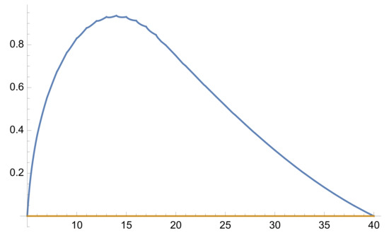
Figure 2. Graphic of $G_1(t,20)$ for $\alpha =\beta =\gamma =1,\delta =0$ (Dirichlet case), $\mu =3/2,a=5$, $b=40$ and $g\equiv 1/100$.

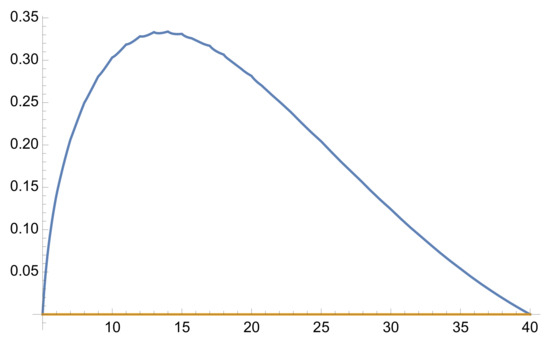
Figure 3. Graphic of $G_2(t,20)$ for $\alpha =\beta =\gamma =1,\delta =0$ (Dirichlet case), $\mu =3/2,a=5$, $b=40$ and $g\equiv 1/100$.

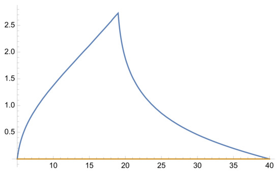
Figure 4. Graphic of the first three iterates of $G(t,20)$ for $\alpha =\beta =\gamma =1,\delta =0$ (Dirichlet case), $\mu =3/2,a=5$, $b=40$ and $g\equiv 1/100$.

Then, we have the following result.

Theorem 3.

Assume that conditions $\left(A0\right)$ and $\left(A1\right)$ are fulfilled, then function $G(t,s)$, defined in (5) as a series of functions, is convergent for $(t,s)\in {\mathbb{N}}_a^b\times {\mathbb{N}}_{a+1}^b$. Moreover, $G(t,s)$ is the Green’s function for the boundary value problem (4).

Proof. 

For any $h\in X$ and $t\in {\mathbb{N}}_a^b$, consider the following linear boundary value problem:

$$\begin{array}{ccc}\hfill -\left({\nabla }_a^{\nu -1}\right(\nabla u\left)\right)\left(t\right)+g\left(t\right)u\left(t\right)& =\hfill & h\left(t\right),t\in {\mathbb{N}}_{a+2}^b,\hfill \\ \hfill \alpha u(a+1)-\beta (\nabla u)(a+1)& =\hfill & 0,\hfill \\ \hfill \gamma u\left(b\right)+\delta (\nabla u)\left(b\right)& =\hfill & 0.\hfill \end{array}$$

(7)

By definition of the Green’s function $G_0$, the solutions u of this problem satisfy the following identity:

$$u\left(t\right)=\sum _{s=a+1}^b{G}_0(t,s)\left[h\left(s\right)-g\left(s\right)u\left(s\right)\right],$$

which is the same to

$$u\left(t\right)+\sum _{s=a+1}^b{G}_0(t,s)g\left(s\right)u\left(s\right)=\sum _{s=a+1}^b{G}_0(t,s)h\left(s\right).$$

(8)

Now, define the operators $T_1:X\to X$ and $T_2:X\to X$ by the following:

$$\begin{array}{ccc}\hfill \left(T_{1}h\right)\left(t\right)& =& \sum _{s=a+1}^b{G}_0(t,s)h\left(s\right),t\in {\mathbb{N}}_a^b,\hfill \\ \hfill \left(T_{2}u\right)\left(t\right)& =& \sum _{s=a+1}^b{G}_0(t,s)g\left(s\right)u\left(s\right),t\in {\mathbb{N}}_a^b.\hfill \end{array}$$

Then, (8) can be expressed as the following:

$$(I+T_2)u=T_{1}h.$$

Using condition (A1) and Theorem 1 the following is true:

$$\begin{array}{cc}\hfill \parallel T_2\parallel =\underset{\parallel u\parallel =1}{max}\parallel T_{2}u\parallel & =\underset{\parallel u\parallel =1}{max}\left[\underset{t\in {\mathbb{N}}_a^b}{max}\left|\left(T_{2}u\right)\left(t\right)\right|\right]\hfill \\ & =\underset{\parallel u\parallel =1}{max}\left[\underset{t\in {\mathbb{N}}_a^b}{max}\left|\sum _{s=a+1}^b{G}_0(t,s)g\left(s\right)u\left(s\right)\right|\right]\hfill \\ & \le \underset{\parallel u\parallel =1}{max}\left[\underset{t\in {\mathbb{N}}_a^b}{max}\sum _{s=a+1}^b{G}_0(t,s)\left|g\left(s\right)\right|\left|u\left(s\right)\right|\right]\hfill \\ & \le \underset{\parallel u\parallel =1}{max}\left[\overline{g}\parallel u\parallel \underset{t\in {\mathbb{N}}_a^b}{max}\sum _{s=a+1}^b{G}_0(t,s)\right]\hfill \\ & <\underset{\parallel u\parallel =1}{max}\left[\overline{g}\parallel u\parallel \Omega \right]=\overline{g}\Omega <1.\hfill \end{array}$$

Then, by Lemma 1, we have the following:

$$u={(I+T_2)}^{-1}{T}_{1}h=\sum _{n=0}^{\infty }{(-T_2)}^n{T}_{1}h.$$

(9)

Arguing in a similar manner than in [20], we can deduce the following:

$$\left({\left(-T_2\right)}^n{T}_{1}h\right)\left(t\right)=\sum _{s=a+1}^b{(-1)}^n{G}_n(t,s)h\left(s\right),t\in {\mathbb{N}}_a^b,n=0,1,2,\dots$$

(10)

Let us see now that the following inequality is fulfilled:

$$\left|{(-1)}^n{G}_n(t,s)\right|<\mathsf{\Lambda }{\left(\overline{g}\Omega \right)}^n,n=0,1,2,\dots$$

(11)

From Theorem 1, we have that (11) holds for $n=0$. Assume now that (11) is true for some $n=k$. Then, the following is true:

$$\begin{array}{cc}\hfill \left|{(-1)}^{k+1}{G}_{k+1}(t,s)\right|& =\left|{(-1)}^{k+1}\sum _{\tau =a+1}^b{G}_0(t,\tau )G_k(\tau ,s)g\left(\tau \right)\right|\hfill \\ & =\left|-\sum _{\tau =a+1}^b{G}_0(t,\tau ){(-1)}^k{G}_k(\tau ,s)g\left(\tau \right)\right|\hfill \\ & \le \sum _{\tau =a+1}^b{G}_0(t,\tau )\left|{(-1)}^k{G}_k(\tau ,s)\right|\left|g\left(\tau \right)\right|\hfill \\ & <\mathsf{\Lambda }{\left(\overline{g}\Omega \right)}^k\overline{g}\sum _{\tau =a+1}^b{G}_0(t,\tau )\hfill \\ & <\mathsf{\Lambda }{\left(\overline{g}\Omega \right)}^k\overline{g}\Omega =\mathsf{\Lambda }{\left(\overline{g}\Omega \right)}^{k+1}.\hfill \end{array}$$

Thus, (11) holds for $n=k+1$. By mathematical induction, (11) holds for any $n=0,1,2,\dots$.

As a direct consequence of previous inequality and condition (A1), we deduce that for all $(t,s)\in {\mathbb{N}}_a^b\times {\mathbb{N}}_{a+1}^b$ the following property is fulfilled:

$$\begin{array}{cc}\hfill \left|G(t,s)\right|=\left|\sum _{n=0}^{\infty }{(-1)}^n{G}_n(t,s)\right|& \le \sum _{n=0}^{\infty }\left|{(-1)}^n{G}_n(t,s)\right|\hfill \\ & <\mathsf{\Lambda }\sum _{n=0}^{\infty }{\left(\overline{g}\Omega \right)}^n=\frac{\mathsf{\Lambda }}{1-\overline{g}\Omega }<\infty ,\hfill \end{array}$$

and, a a consequence, $G(t,s)$ converges on ${\mathbb{N}}_a^b\times {\mathbb{N}}_{a+1}^b$.

Finally, expressions (5), (9) and (10) imply that for all $t\in {\mathbb{N}}_a^b$ the following equality is fulfilled:

$$\begin{array}{cc}\hfill u\left(t\right)=\sum _{n=0}^{\infty }\left[\sum _{s=a+1}^b{(-1)}^n{G}_n(t,s)h\left(s\right)\right]& =\sum _{s=a+1}^b\left[\sum _{n=0}^{\infty }{(-1)}^n{G}_n(t,s)\right]h\left(s\right)\hfill \\ & =\sum _{s=a+1}^{b}G(t,s)h\left(s\right).\hfill \end{array}$$

(12)

It is not difficult to verify that any function defined by (12) is a solution of the boundary value problem (7). So we conclude that problem (7) has a unique solution and, as a consequence, G is its related Green’s function. □

Lemma 2.

Assume conditions $\left(A0\right)$ and $\left(A1\right)$. Let G be defined by (5) and the following:

$$\overline{G}\left(s\right)=\frac{G_0(\rho \left(s\right),s)}{1-\overline{g}\Omega },s\in {\mathbb{N}}_{a+1}^b.$$

(13)

Then,

$$\left|G(t,s)\right|\le \overline{G}\left(s\right),(t,s)\in {\mathbb{N}}_a^b\times {\mathbb{N}}_{a+1}^b.$$

Proof. 

First, we prove the following:

$$\left|{(-1)}^n{G}_n(t,s)\right|<G(s-1,s){\left(\overline{g}\Omega \right)}^n,s\in {\mathbb{N}}_{a+1}^b,n=0,1,2,\dots$$

(14)

Theorem 1 implies that inequality (14) is true for $n=0$.

Assume now that (14) holds for some $n=k$. We will show that (14) holds for $n=k+1$. Consider the following:

$$\begin{array}{cc}\hfill \left|{(-1)}^{k+1}{G}_{k+1}(t,s)\right|& =\left|{(-1)}^{k+1}\sum _{\tau =a+1}^b{G}_0(t,\tau )G_k(\tau ,s)g\left(\tau \right)\right|\hfill \\ & =\left|-\sum _{\tau =a+1}^b{G}_0(t,\tau ){(-1)}^k{G}_k(\tau ,s)g\left(\tau \right)\right|\hfill \\ & \le \sum _{\tau =a+1}^b{G}_0(t,\tau )\left|{(-1)}^k{G}_k(\tau ,s)\right|\left|g\left(\tau \right)\right|\hfill \\ & <G(s-1,s){\left(\overline{g}\Omega \right)}^k\overline{g}\sum _{\tau =a+1}^b{G}_0(t,\tau )\hfill \\ & <G(s-1,s){\left(\overline{g}\Omega \right)}^k\overline{g}\Omega =G(s-1,s){\left(\overline{g}\Omega \right)}^{k+1}.\hfill \end{array}$$

Thus, (14) holds for $n=k+1$ and the inequalities are deduced from mathematical induction.

Now, from (5), (13) and (14), for $s\in {\mathbb{N}}_{a+1}^b$, we obtain the following:

$$\begin{array}{cc}\hfill \left|G(t,s)\right|=\left|\sum _{n=0}^{\infty }{(-1)}^n{G}_n(t,s)\right|& \le \sum _{n=0}^{\infty }\left|{(-1)}^n{G}_n(t,s)\right|\hfill \\ & <G(s-1,s)\sum _{n=0}^{\infty }{\left(\overline{g}\Omega \right)}^n\hfill \\ & =\frac{G_0(\rho \left(s\right),s)}{1-\overline{g}\Omega }=\overline{G}\left(s\right),\hfill \end{array}$$

and the proof is complete. □

From the previous result, we deduce the following consequence for $g\le 0$.

Corollary 1.

Assume that condition (A) is fulfilled and

$$-\overline{g}<g\left(t\right)\le 0,t\in {\mathbb{N}}_a^b.$$

Then, $G(t,s)\ge 0$ for each $(t,s)\in {\mathbb{N}}_a^b\times {\mathbb{N}}_{a+1}^b$.

Proof. 

From Theorem 1, we know that $G_0(t,s)\ge 0$ for each $(t,s)\in {\mathbb{N}}_a^b\times {\mathbb{N}}_{a+1}^b$. The result follows immediately from (5) and (6). □

4. Existence of Solutions

In this section, we derive two existence results for the nonlinear problem (1). Define the operator $T:X\to X$ (X defined in previous section) by the following:

$$(Tu)\left(t\right)=\sum _{s=a+1}^{b}G(t,s)f(s,u\left(s\right)),t\in {\mathbb{N}}_a^b.$$

(15)

In view of (12), it is clear that u is a fixed point of T if and only if u is a solution of (1).

For any $R>0$ given, we define the following set:

$${\mathcal{K}}_R=\{u\in X:\parallel u\parallel <R\}.$$

Clearly, ${\mathcal{K}}_R$ is a non-empty open subset of X, $0\in {\mathcal{K}}_R$ and $T:\overline{{\mathcal{K}}_R}\to X$.

Now, denoting by

$$\underset{t\in {\mathbb{N}}_a^b}{max}\left|f(t,0)\right|=M\mathrm{and}\sum _{s=a+1}^b\overline{G}\left(s\right)=K(>0),$$

we enunciate the following list of assumptions:

(A2)

$f:{\mathbb{N}}_a^b\times \mathbb{R}\to \mathbb{R}$ is continuous;

(A3)

f satisfies the Lipschitz condition with respect to the second variable with the Lipschitz constant L on ${\mathbb{N}}_a^b\times {\mathcal{K}}_R$. That is, for all $(t,u)$, $(t,v)\in {\mathbb{N}}_a^b\times [-R,R]$, the following inequality holds:

$$\left|f\right(t,u)-f(t,v\left)\right|\le L|u-v|.$$

(A4)

There exists a continuous function $\sigma :{\mathbb{N}}_a^b\to {\mathbb{R}}^{+}$ and a continuous nondecreasing function $\psi :{\mathbb{R}}^{+}\to {\mathbb{R}}^{+}$ such that

$$\left|f(t,u)\right|\le \sigma \left(t\right)\psi \left(\left|u\right|\right),(t,u)\in {\mathbb{N}}_a^b\times \mathbb{R}.$$

(A5)

$0<LK<1$.

First, we present a nonlinear alternative of Leray–Schauder for contractive maps.

Theorem 4.

(Theorem 3.2) Suppose U is an open subset of a Banach space X,$0\in U$and$F:\overline{U}\to X$a contraction with$F\left(\overline{U}\right)$bounded [24]. Then, either of the following is true:

(1)

F has a fixed point in $\overline{U}$.

(2)

There exist $\lambda \in (0,1)$ and $u\in \partial U$ with $u=\lambda Fu$,

holds.

Now, we establish sufficient conditions on existence of solutions for (1) using Theorem 4.

Theorem 5.

Assume (A0)–(A3), (A5) hold. If we choose R such that

$$R\ge \frac{MK}{1-L{K}^{\prime }}$$

(16)

then the boundary value problem (1) has a solution in $\overline{{\mathcal{K}}_R}$.

Proof. 

First, we show that T is a contraction. To see this, let u, $v\in \overline{{\mathcal{K}}_R}$, $t\in {\mathbb{N}}_a^b$, and consider the following:

$$\begin{array}{cc}\hfill \left|\left(Tu\right)\left(t\right)-\left(Tv\right)\left(t\right)\right|& =\left|\sum _{s=a+1}^{b}G(t,s)\left[f(s,u(s\left)\right)-f(s,v(s\left)\right)\right]\right|\hfill \\ & \le \sum _{s=a+1}^b\left|G(t,s)\right|\left|f(s,u(s\left)\right)-f(s,v(s\left)\right)\right|\hfill \\ & \le L\sum _{s=a+1}^b\overline{G}\left(s\right)\left|u\left(s\right)-v\left(s\right)\right|\hfill \\ & \le LK\parallel u-v\parallel ,\hfill \end{array}$$

implying that

$$\parallel Tu-Tv\parallel \le LK\parallel u-v\parallel .$$

Since

$$0<LK<1,$$

it follows that T is a contraction.

Next, we prove that $T\left(\overline{{\mathcal{K}}_R}\right)$ is bounded.

To see this, let $u\in \overline{{\mathcal{K}}_R}$ ($\parallel u\parallel \le R$), $t\in {\mathbb{N}}_a^b$, and consider the following:

$$\begin{array}{cc}\hfill \left|\left(Tu\right)\left(t\right)\right|& =\left|\sum _{s=a+1}^{b}G(t,s)f(s,u\left(s\right))\right|\hfill \\ & \le \sum _{s=a+1}^b\left|G(t,s)\right|\left|f(s,v(s\left)\right)\right|\hfill \\ & =\sum _{s=a+1}^b\left|G(t,s)\right|\left|f(s,u(s\left)\right)-f(s,0)+f(s,0)\right|\hfill \\ & \le \sum _{s=a+1}^b\overline{G}\left(s\right)\left|f(s,u(s\left)\right)-f(s,0)\right|+\sum _{s=a+1}^b\overline{G}\left(s\right)\left|f(s,0)\right|\hfill \\ & \le L\sum _{s=a+1}^b\overline{G}\left(s\right)\left|u\left(s\right)\right|+M\sum _{s=a+1}^b\overline{G}\left(s\right)\hfill \\ & \le LK\parallel u\parallel +MK\le \left[LR+M\right]K,\hfill \end{array}$$

implying the following:

$$\parallel Tu\parallel \le \left[LR+M\right]K.$$

Thus, $T\left(\overline{{\mathcal{K}}_R}\right)$ bounded.

Now, suppose there exist $v\in \partial {\mathcal{K}}_R$ ($\parallel v\parallel =R$) and $\lambda \in (0,1)$ such that

$$v=\lambda Tv.$$

(17)

Using the definition of T in (17) and arguing as before, we obtain the following:

$$\begin{array}{cc}\hfill \left|v\left(t\right)\right|& =\left|\lambda \left(Tv\right)\left(t\right)\right|\le \left[LR+M\right]\lambda K<\left[LR+M\right]K,t\in {\mathbb{N}}_a^b,\hfill \end{array}$$

which implies the following:

$$R=\parallel v\parallel <\left[LR+M\right]K$$

or, which is the same,

$$R<\frac{MK}{1-LK},$$

in contradiction with (16).

Hence, by Theorem 4, we deduce that operator T has a fixed point in $\overline{{\mathcal{K}}_R}$ and the proof is complete. □

Remark 1.

We note that in the previous result, if $M=0$ then we have that $u\equiv 0$ on $[0,1]$ is a solution of problem (1). On the contrary, if $M>0$ the obtained function is non trivial on $[0,1]$

Next, we enunciate a nonlinear alternative of Leray–Schauder for continuous and compact maps.

Theorem 6.

Let E be a Banach space, C a closed, convex subset of E, U an open subset of C and$0\in U$[24] (Theorem 6.6). Suppose that$F:\overline{U}\to C$is a continuous, compact map. Then, either of the following is true:

(1)

F has a fixed point in $\overline{U}$, or

(2)

there is a $u\in \partial U$ and $\lambda \in (0,1)$ with $u=\lambda Fu$.

Now, we establish sufficient conditions on existence of solutions for (1) using Theorem 6.

Theorem 7.

Assume that conditions (A0)–(A2), and (A4) hold. If we choose R such that

$$\frac{R}{K\parallel \sigma \parallel \psi \left(R\right)}\ge 1,$$

(18)

then the boundary value problem (1) has a solution in $\overline{{\mathcal{K}}_R}$.

Proof. 

Since T is a summation operator on a discrete finite set, it is trivially continuous and compact. Now, suppose that there exist $v\in \partial {\mathcal{K}}_R$ ($\parallel v\parallel =R$) and $\lambda \in (0,1)$ such that (17) holds. Using the definition of T in (17), we obtain the following:

$$\begin{array}{cc}\hfill \left|v\left(t\right)\right|& =\left|\lambda \left(Tv\right)\left(t\right)\right|\hfill \\ & =\left|\lambda \sum _{s=a+1}^{b}G(t,s)f(s,v\left(s\right))\right|\hfill \\ & \le \lambda \sum _{s=a+1}^b\left|G(t,s)\right|\left|f(s,v(s\left)\right)\right|\hfill \\ & \le \lambda \sum _{s=a+1}^b\left|G(t,s)\right|\sigma \left(s\right)\psi \left(\left|v\left(s\right)\right|\right)\hfill \\ & \le \lambda \parallel \sigma \parallel \psi \left(\parallel v\parallel \right)\sum _{s=a+1}^b\overline{G}\left(s\right)\hfill \\ & <K\parallel \sigma \parallel \psi \left(\parallel v\parallel \right).\hfill \end{array}$$

So, we deduce the following:

$$R=\parallel v\parallel <K\parallel \sigma \parallel \psi \left(\parallel v\parallel \right).$$

Thus,

$$\frac{R}{K\parallel \sigma \parallel \psi \left(R\right)}<1.$$

This is a contradiction to (18).

Hence, by Theorem 6, the boundary value problem (1) has a solution in $\overline{{\mathcal{K}}_R}$. The proof is complete. □

Remark 2.

Note that since we have that

$$\underset{t\in {\mathbb{N}}_a^b}{max}{G}_0\left(t,s\right)<\mathsf{\Lambda }$$

we can set the following:

$$\overline{K}=\frac{\mathsf{\Lambda }}{1-\overline{g}\Omega }\left(b-a\right)>\sum _{s=a+1}^b\overline{G}\left(s\right)=K.$$

Thus, we can use $\overline{K}$ instead of K everywhere and we do not need to calculate the Green’s function at all.

Indeed, in (A5), if we have $0<L\overline{K}<1,$ this implies that $0<LK<1.$

In Theorem 4.2, if we choose $R\ge \frac{M\overline{K}}{1-L\overline{K}},$ then we will also have that $R\ge \frac{MK}{1-LK}$ since $\frac{M\overline{K}}{1-L\overline{K}}\ge \frac{MK}{1-LK}.$

Finally, in Theorem 4.4, if we choose $\frac{R}{\overline{K}∥\sigma ∥\psi \left(R\right)}\ge 1,$ then we will also have that $\frac{R}{K∥\sigma ∥\psi \left(R\right)}\ge 1$ since $\frac{R}{K∥\sigma ∥\psi \left(R\right)}\ge \frac{R}{\overline{K}∥\sigma ∥\psi \left(R\right)}.$

5. Examples

In the section, we present some examples to illustrate the applicability of our main results.

Problem 1.

Consider the following nabla fractional boundary value problem:

$$\begin{array}{ccc}\hfill -\left({\nabla }_0^{1/2}\right(\nabla u\left)\right)\left(t\right)+\frac{e^{-t}}{10}u\left(t\right)& =\hfill & \frac{1}{200}sin\left(u\left(t\right)+t\right),t\in {\mathbb{N}}_2^6,\hfill \\ \hfill u\left(0\right)=u\left(6\right)& =\hfill & 0.\hfill \end{array}$$

(19)

Here, $\alpha =1$, $\beta =1$, $\gamma =1$ and $\delta =0$, $a=0$, $b=6$ and $\nu =3/2$.

In addition, $g\left(t\right)=e^{-t}/10$ and $f(t,u)=(sin\left(u+t\right))/200$. Clearly, $g:{\mathbb{N}}_0^6\to \mathbb{R}$; $f:{\mathbb{N}}_0^6\times \mathbb{R}\to \mathbb{R}$ is continuous and satisfies Lipschitz condition with respect to u on ${\mathbb{N}}_0^6\times \mathbb{R}$ with Lipschitz constant $L=0.005$.

We have $\xi =H_{0.5}\left(6,0\right)\approx 2.7071$, $\mathsf{\Lambda }=H_{0.5}\left(6,0\right)\approx 2.7071$, $\Omega =H_2\left(6,1\right)=3$ and $\overline{g}=0.1$ so that $\left|g\left(t\right)\right|\le \overline{g}<\frac{1}{\Omega }$. Further,

$$\overline{K}=\frac{\mathsf{\Lambda }}{1-\overline{g}\Omega }(b-a)\approx 23.2037.$$

Observe that $0<L\overline{K}\approx 0.116<1$. Additionally,

$$M=\underset{t\in {\mathbb{N}}_0^6}{max}\left|f(t,0)\right|=\underset{t\in {\mathbb{N}}_0^6}{max}\left|\frac{sint}{200}\right|\approx 0.00479462137.$$

If we choose

$$R\ge \frac{M\overline{K}}{1-L\overline{K}}\approx 0.12585176,$$

then by Theorem 5 and Remark 2, the boundary value problem (19) has a solution in $\overline{{\mathcal{K}}_R}$.

Problem 2.

Consider the following nabla fractional boundary value problem:

$$\begin{array}{ccc}\hfill -\left({\nabla }_0^{1/2}\right(\nabla u\left)\right)\left(t\right)+\frac{1}{20(t+1)}u\left(t\right)& =\hfill & \frac{u^2\left(t\right)}{10(t^2+10)},t\in {\mathbb{N}}_2^9,\hfill \\ \hfill u\left(0\right)+u\left(1\right)& =\hfill & 0,\hfill \\ \hfill u\left(8\right)+u\left(9\right)& =\hfill & 0.\hfill \end{array}$$

(20)

Here, $\alpha =2$, $\beta =1$, $\gamma =2$ and $\delta =-1$ such that ${\alpha }^2+{\beta }^2>0$ and ${\gamma }^2+{\delta }^2>0$, $a=0$, $b=9$ and $\nu =3/2$.

In addition, $g\left(t\right)=\frac{1}{20(t+1)}$ and $f(t,u)=\frac{u^2\left(t\right)}{10(t^2+10)}$. Clearly, $g:{\mathbb{N}}_0^9\to \mathbb{R}$ and $f:{\mathbb{N}}_0^9\times \mathbb{R}\to \mathbb{R}$ are continuous.

We have $\xi \approx 10.9616$, $\mathsf{\Lambda }\approx 2.9403$, $\Omega =15.8396$ and $\overline{g}\approx 0.05$ so that $\left|g\left(t\right)\right|\le \overline{g}<\frac{1}{\Omega }$. Further,

$$\overline{K}=\frac{\mathsf{\Lambda }}{1-\overline{g}\Omega }(b-a)\approx 127.2245.$$

In addition,

$$\left|f(t,u)\right|\le \sigma \left(t\right)\psi \left(\left|u\right|\right),(t,u)\in {\mathbb{N}}_0^9\times \mathbb{R},$$

where $\sigma \left(t\right)=\frac{1}{10(t^2+10)}$ and $\psi \left(x\right)=x^2$. Observe that $\sigma :{\mathbb{N}}_0^9\to {\mathbb{R}}^{+}$ is continuous and $\psi :{\mathbb{R}}^{+}\to {\mathbb{R}}^{+}$ is continuous non-decreasing with

$$\parallel \sigma \parallel =\underset{t\in {\mathbb{N}}_0^9}{max}\left|\sigma \left(t\right)\right|=0.001.$$

If we choose

$$\frac{R}{\overline{K}∥\sigma ∥\psi \left(R\right)}\ge 1,$$

that is, $R\le 7.8616$, then by Theorem 7 and Remark 2, the boundary value problem (19) has a solution in $\overline{{\mathcal{K}}_R}$.

References

- Gray, H.L.; Zhang, N.F. On a new definition of the fractional difference. Math. Comput. 1988, 50, 513–529. [Google Scholar] [CrossRef]
- Atıcı, F.M.; Eloe, P.W. Discrete fractional calculus with the nabla operator. Electron. J. Qual. Theory Differ. Equ. 2009, 12. [Google Scholar] [CrossRef]
- Anastassiou, G.A. Nabla discrete fractional calculus and nabla inequalities. Math. Comput. Model. 2010, 51, 562–571. [Google Scholar] [CrossRef] [Green Version]
- Goodrich, C.; Peterson, A.C. Discrete Fractional Calculus; Springer: Cham, Switzerland, 2015. [Google Scholar]
- Hill, G.W. On the part of the motion of the lunar perigee which is a function of the mean motions of the Sun and the Moon. Acta Math. 1886, 8, 1–36. [Google Scholar] [CrossRef]
- Cabada, A.; Cid, J.Á.; López-Somoza, L. Maximum Principles for the Hill’s Equation; Academic Press: London, UK, 2018; 238p. [Google Scholar]
- Magnus, W.; Winkler, S. Hill’s Equation; Corrected Reprint of the 1966 Edition; Dover Publications, Inc.: New York, NY, USA, 1979; 129p. [Google Scholar]
- Brackins, A. Boundary Value Problems of Nabla Fractional Difference Equations. Ph.D. Thesis, The University of Nebraska-Lincoln, Lincoln, NE, USA, 2014; 92p. [Google Scholar]
- Ahrendt, K.; Kissler, C. Cameron Green’s function for higher-order boundary value problems involving a nabla Caputo fractional operator. J. Differ. Equ. Appl. 2019, 25, 788–800. [Google Scholar] [CrossRef] [Green Version]
- Chen, C.; Bohner, M.; Jia, B. Existence and uniqueness of solutions for nonlinear Caputo fractional difference equations. Turk. J. Math. 2020, 44, 857–869. [Google Scholar] [CrossRef]
- Gholami, Y.; Ghanbari, K. Coupled systems of fractional ∇-difference boundary value problems. Differ. Equ. Appl. 2016, 8, 459–470. [Google Scholar] [CrossRef] [Green Version]
- Goodrich, C.S. Existence of a positive solution to a class of fractional differential equations. Appl. Math. Lett. 2010, 23, 1050–1055. [Google Scholar] [CrossRef] [Green Version]
- Goodrich, C.S. Existence and uniqueness of solutions to a fractional difference equation with nonlocal conditions. Comput. Math. Appl. 2011, 61, 191–202. [Google Scholar] [CrossRef]
- Ikram, A. Lyapunov inequalities for nabla Caputo boundary value problems. J. Differ. Equ. Appl. 2019, 25, 757–775. [Google Scholar] [CrossRef] [Green Version]
- Baoguo, J.; Erbe, L.; Goodrich, C.; Peterson, A. The relation between nabla fractional differences and nabla integer differences. Filomat 2017, 31, 1741–1753. [Google Scholar] [CrossRef]
- Jonnalagadda, J.M. On two-point Riemann-Liouville type nabla fractional boundary value problems. Adv. Dyn. Syst. Appl. 2018, 13, 141–166. [Google Scholar]
- Liu, X.; Jia, B.; Gensler, S.; Erbe, L.; Peterson, A. Convergence of approximate solutions to nonlinear Caputo nabla fractional difference equations with boundary conditions. Electron. J. Differ. Equ. 2020, 2020, 1–19. [Google Scholar]
- St. Goar, J. A Caputo Boundary Value Problem in Nabla Fractional Calculus. Ph.D. Thesis, The University of Nebraska-Lincoln, Lincoln, NE, USA, 2016; 112p. [Google Scholar]
- Graef, J.R.; Kong, L.; Kong, Q.; Wang, M. Existence and uniqueness of solutions for a fractional boundary value problem with Dirichlet boundary condition. Electron. J. Qual. Theory Differ. Equ. 2013, 2013, 1–11. [Google Scholar] [CrossRef]
- Cabada, A.; Dimitrov, N. Non-trivial solutions of non-autonomous Dirichlet fractional discrete problems. Fract. Calc. Appl. Anal. 2020, 23, 980–995. [Google Scholar] [CrossRef]
- Jonnalagadda, J.M. Existence results for solutions of nabla fractional boundary value problems with general boundary conditions. Adv. Theory Nonlinear Anal. Appl. 2020, 4, 29–42. [Google Scholar] [CrossRef] [Green Version]
- Jonnalagadda, J.M. On a nabla fractional boundary value problem with general boundary conditions. AIMS Math. 2020, 5, 204–215. [Google Scholar] [CrossRef]
- Zeidler, E. Nonlinear Functional Analysis and Its Applications. I. Fixed-Point Theorems; Wadsack, P.R., Translator; Springer: New York, NY, USA, 1986. [Google Scholar]
- Agarwal, R.P.; Meehan, M.; O’regan, D. Fixed Point Theory and Applications. Cambridge Tracts in Mathematics; Cambridge University Press: Cambridge, UK, 2001; Volume 141. [Google Scholar]
Publisher’s Note: MDPI stays neutral with regard to jurisdictional claims in published maps and institutional affiliations. |
© 2021 by the authors. Licensee MDPI, Basel, Switzerland. This article is an open access article distributed under the terms and conditions of the Creative Commons Attribution (CC BY) license (https://creativecommons.org/licenses/by/4.0/).