Generalized Eigenvalue Proximal Support Vector Machine for Functional Data Classification

Abstract

Functional data analysis has become a research hotspot in the field of data mining. Traditional data mining methods regard functional data as a discrete and limited observation sequence, ignoring the continuity. In this paper, the functional data classification is addressed, proposing a functional generalized eigenvalue proximal support vector machine (FGEPSVM). Specifically, we find two nonparallel hyperplanes in function space, a positive functional hyperplane, and a functional negative hyperplane. The former is closest to the positive functional data and furthest from the negative functional data, while the latter has the opposite properties. By introducing the orthonormal basis, the problem in function space is transformed into the ones in vector space. It should be pointed out that the higher-order derivative information is applied from two aspects. We apply the derivatives alone or the weighted linear combination of the original function and the derivatives. It can be expected that to improve the classification accuracy by using more data information. Experiments on artificial datasets and benchmark datasets show the effectiveness of our FGEPSVM for functional data classification.

1. Introduction

The concept of functional data was first put forward by Ramsay and showed that functional data can be obtained through advanced equipment [1]. Then, these data can be regarded as dynamic and continuous data, rather than static and discrete data in the traditional data analysis. Ramsay and Dalzel further proposed a systematic tool for functional data analysis (FDA) and promoted some traditional analysis methods [2]. Ramsay and Silverman popularized functional data analysis and have brought widespread attention for the last two decades [3]. In recent years, with the improvement of data acquisition technology and data storage capacity, more and more complex data are constantly appearing, presented in the form of functions. These data appear in every aspect of human production and life, such as speech recognition, spectral analysis, meteorology, etc. Functional data contains more complete and sufficient information, which can avoid information loss caused by discrete data. Therefore, it has become a research hotspot [4,5,6,7,8].

We deal with the problem of classifying functional data. There are numerous functional data classification problems [9,10,11,12,13]. For example, a doctor can determine whether the arteries of a patient are narrowly based on a Doppler ultrasonography, and marble can be automatically graded using the spectral curve. Many scholars have researched this area. Rossi and Villa showed how to use support vector machines (SVMs) for functional data classification [14]. Li and Yu suggested a classification and feature extraction method on functional data where the predictor variables are curves; it combines the classical linear discriminant analysis and SVM [15]. Muñoz proposed a functional analysis technique to obtain finite-dimensional representations of functional data. The key idea is to consider each functional datum as a point in public function space and then project these points onto a Reproducing Kernel Hilbert Space with SVM [16]. Chang proposed a new semi-metric based on wavelet thresholding for functional data classification [17]. Martin-Barragan faced the problem of obtaining an SVM-based classifier for functional data with good classification ability and provides a classifier that is easy to interpret [18]. Blanquero proposed a new approach to optimally select the most informative time instants in multivariate functional data to get reasonable classification rates [19]. Moreover, other researchers applied different approaches to solve the functional data classification problems [20,21,22].

SVMs are one of the most comment methods to address classification. According to supervised learning, it is a generalized linear classifier. Its decision boundary maximizes the margin between the hyperplane of the training set [23]. The pioneering work can be traced to a study by Vapnik and Lerner in 1963 [24]. Vapnik and Chervonenkis established the linear SVM with a hard margin in 1964 [25]. Boser, Guyon, and Vapnik obtained the nonlinear SVM through the kernel method in 1992 [26]. Cortes and Vapnik proposed the nonlinear SVM of soft margins in 1995 [27], and this study received attention and citation after publication. SVM seeks a hyperplane and finally solves a quadratic programming problem in the dual space. As an extension of the SVM, the nonparallel support vector machine (NPSVM) constructs corresponding support hyperplanes for each class to describe the difference in data distribution between different classes [28,29,30,31]. The idea was first proposed by Magasarian in 2006, who came up with a generalized eigenvalue proximal support vector machine (GEPSVM) [32]. The model obtained two nonparallel hyperplanes by solving two generalized eigenvalue problems [33]. GEPSVM has two advantages over SVM. The first is the computation time, the former is solving a pair of generalized eigenvalue problems, while the latter is solving a quadratic programming problem, obviously because the former has low computational complexity. Next, GEPSVM performs better than SVM on crossed datasets.

This paper considers the binary functional data classification. Inspired by the success of GEPSVM, our proposal finds two nonparallel hyperplanes in function space. Each of the functional hyperplanes is generated such that it is close to the functional data in one class while is far away from the other class. This yields the optimization problem in function space. Then it is transformed into the vector space through the orthonormal basis. It is worthwhile to mention that our methodology is not only restricted to the original function. Indeed, the approach proposed here can be directly applied to higher-order derivatives. Only the functional data can employ the higher-order derivative information, which is impossible for the discrete data in the traditional data analysis because the discrete data does not have the property of functions. We mainly consider higher-order derivative information from two aspects. First, using derivative alone can improve the classification accuracy when the difference between original functions may not be distinct in the training set. Moreover, we employ the weighted linear combination of derivatives, which contains more information to improve the classification accuracy. The former is a particular case of the latter. Our model is based on the weighted linear combination of derivatives, and this paper considers the original function, first derivative, and second derivative in the experiment. The numerical experiment shows that the higher-order derivative information will be crucial in the classifier performance. Moreover, when we apply the weighted linear combination of the original function and the derivatives, the performance of our method is excellent on some datasets as well, which indicates that it is feasible to employ the weighted linear combination. Two main advantages are obtained from our concept. One is the classification accuracy of FGEPSVM on some datasets is better than that of SVM, such as crossed datasets. Moreover, given that the computational complexity of GEPSVM is much lower than SVM, especially when dealing with large-scale datasets.

The overall structure of this paper is as follows. Section 1 introduces the research background and significance. Section 2 reviews the related work. Section 3 introduces the functional data and proposes our method, FGEPSM, to solve the functional data classification. Section 4 is the numerical experiment, which is divided into three parts. The first part is an experiment on artificial datasets, which demonstrates the feasibility of the proposed method. In the second part, experiments on classical functional datasets are carried out to further illustrate the effectiveness of our proposal. The last part is the parameter analysis, which discusses the influence of the important parameter on classification accuracy. Finally, the summary part briefly describes the content of this paper and the proposed methods.

2. Related Work

Here, we introduce the basic notation. Throughout this paper, uppercase and lowercase characters are used to denote matrices and vectors. ${\mathbb{R}}^{m\times n}$ and ${\mathbb{R}}^n$ denote the set of $m\times n$ matrices and n-dimensional vectors, respectively. The inner product of two vectors $\mathit{x}$ and $\mathit{y}$ in the n-dimensional real space ${\mathbb{R}}^n$ is defined by $<\mathit{x},\mathit{y}>={\mathit{x}}^T\mathit{y}$. Furthermore, the inner product of two functions $x\left(t\right)$ and $y\left(t\right)$ in the square-integrable function space $L^2\left(T\right)$ is denoted by $<x\left(t\right),y\left(t\right)>={\int }_{T}x\left(t\right)y\left(t\right)dt$. The norm in this paper refers to the 2-norm of a vector, which is denoted by $\parallel x\parallel ={({\displaystyle \sum _{i=1}^n}{x}_i^2)}^{\frac{1}{2}}$, where $\mathit{x}={(x_1,x_2,\dots ,x_n)}^T$.

Our work is closely related with the generalized eigenvalue proximal support vector machine (GEPSVM) [32]. Given a training set

$$T=\{({\mathit{x}}_1,y_1),\dots ,({\mathit{x}}_{m_{+}},y_{m_{+}}),({\mathit{x}}_{m_{+}+1},y_{m_{+}+1}),\dots ,({\mathit{x}}_{m_{+}+m_{-}},y_{m_{+}+m_{-}})\},$$

(1)

where ${\mathit{x}}_i\in {\mathbb{R}}^n$, $i=1,\dots ,m_{+},m_{+}+1,\dots ,m_{+}+m_{-}$. $y_1=\cdots =y_{m_{+}}=+1,y_{m_{+}+1}=\cdots =y_{m_{+}+m_{-}}=-1$. The goal of GEPSVM is to find two nonparallel hyperplanes in $R^n$

$$<{\mathit{w}}_{+},\mathit{x}>+b_{+}=0,$$

(2)

and

$$<{\mathit{w}}_{-},\mathit{x}>+b_{-}=0,$$

(3)

where ${\mathit{w}}_{+},{\mathit{w}}_{-}\in {\mathbb{R}}^n$, $b_{+},b_{-}\in \mathbb{R}$. The positive plane (2) is closest to the data points of class $+1$ and furthest from the data points in class $-1$, while the negative plane (3) is closest to the points in class $-1$ and furthest from the points in class $+1$. Thus, the optimization problems are formulated as

$$\underset{({\mathit{w}}_{+}^T,b_{+})\ne 0}{min}\frac{{\displaystyle \sum _{i=1}^{m_{+}}}{(<{\mathit{w}}_{+},{\mathit{x}}_{\mathit{i}}>+b_{+})}^2+\Omega \left(f_{+}\right)}{{\displaystyle \sum _{i=m_{+}+1}^{m_{+}+m_{-}}}{(<{\mathit{w}}_{+},{\mathit{x}}_{\mathit{i}}>+b_{+})}^2},$$

(4)

and

$$\underset{({\mathit{w}}_{-}^T,b_{-})\ne 0}{min}\frac{{\displaystyle \sum _{i=m_{+}+1}^{m_{+}+m_{-}}}{(<{\mathit{w}}_{-},{\mathit{x}}_{\mathit{i}}>+b_{-})}^2+\Omega \left(f_{-}\right)}{{\displaystyle \sum _{i=1}^{m_{+}}}{(<{\mathit{w}}_{-},{\mathit{x}}_{\mathit{i}}>+b_{-})}^2},$$

(5)

where $f_{+}=<{\mathit{w}}_{+},\mathit{x}>+b_{+}$, $f_{-}=<{\mathit{w}}_{-},\mathit{x}>+b_{-}$. $\Omega \left(f_{+}\right)$ and $\Omega \left(f_{-}\right)$ are regularization terms.

We organize the $m_{+}$ data points of Class $+1$ by ${\mathit{X}}_{+}={({\mathit{x}}_1,\dots ,{\mathit{x}}_{m_{+}})}^T\in {\mathbb{R}}^{m_{+}\times n}$ and the $m_{-}$ data points of Class $-1$ by ${\mathit{X}}_{-}={({\mathit{x}}_{m_{+}+1},\dots ,{\mathit{x}}_{m_{+}+m_{-}})}^T\in {\mathbb{R}}^{m_{-}\times n}$. Selecting the Tikhonov regularization terms [34] to be $\Omega \left(f_{+}\right)=\delta {∥\left(\begin{array}{c}{\mathit{w}}_{+}\\ b_{+}\end{array}\right)∥}^2$ and $\Omega \left(f_{-}\right)=\delta {∥\left(\begin{array}{c}{\mathit{w}}_{-}\\ b_{-}\end{array}\right)∥}^2$ with a nonnegative parameter $\delta$, (4) and (5) can be written as

$$\underset{({\mathit{w}}_{+}^T,b_{+})\ne 0}{min}\frac{{∥{\mathit{X}}_{+}{\mathit{w}}_{+}+b_{+}{\mathit{e}}_{+}∥}^2+\delta {∥\left(\begin{array}{c}{\mathit{w}}_{+}\\ b_{+}\end{array}\right)∥}^2}{{∥{\mathit{X}}_{-}{\mathit{w}}_{+}+b_{+}{\mathit{e}}_{-}∥}^2},$$

(6)

and

$$\underset{({\mathit{w}}_{-}^T,b_{-})\ne 0}{min}\frac{{∥{\mathit{X}}_{-}{\mathit{w}}_{-}+b_{-}{\mathit{e}}_{-}∥}^2+\delta {∥\left(\begin{array}{c}{\mathit{w}}_{-}\\ b_{-}\end{array}\right)∥}^2}{{∥{\mathit{X}}_{+}{\mathit{w}}_{-}+b_{-}{\mathit{e}}_{+}∥}^2},$$

(7)

where ${\mathit{e}}_{+}$ and ${\mathit{e}}_{-}$ are all ones vectors with length $m_{+}$ and $m_{-}$, respectively.

Starting from the identity matrix $\mathit{I}$ of appropriate dimensions, define the symmetric matrices $\mathit{G}$, $\mathit{H}$, $\mathit{R}$, $\mathit{S}\in {\mathbb{R}}^{(n+1)\times (n+1)}$

$$\begin{array}{c}\hfill \mathit{G}={({\mathit{X}}_{+},{\mathit{e}}_{+})}^T({\mathit{X}}_{+},{\mathit{e}}_{+})+\delta \mathit{I},\mathit{H}={({\mathit{X}}_{-},{\mathit{e}}_{-})}^T({\mathit{X}}_{-},{\mathit{e}}_{-}),\\ \hfill \mathit{R}={({\mathit{X}}_{-},{\mathit{e}}_{-})}^T({\mathit{X}}_{-},{\mathit{e}}_{-})+\delta \mathit{I},\mathit{S}={({\mathit{X}}_{+},{\mathit{e}}_{+})}^T({\mathit{X}}_{+},{\mathit{e}}_{+}),\end{array}$$

(8)

and the vectors ${\mathit{z}}_{+}$, ${\mathit{z}}_{-}\in {\mathbb{R}}^{(n+1)}$

$${\mathit{z}}_{+}=\left(\begin{array}{c}{\mathit{w}}_{+}\\ b_{+}\end{array}\right),{\mathit{z}}_{-}=\left(\begin{array}{c}{\mathit{w}}_{-}\\ b_{-}\end{array}\right),$$

(9)

then the optimization problems become

$$\underset{{\mathit{z}}_{+}\ne 0}{min}\frac{{\mathit{z}}_{+}^T\mathit{G}{\mathit{z}}_{+}}{{\mathit{z}}_{+}^T\mathit{H}{\mathit{z}}_{+}},$$

(10)

and

$$\underset{{\mathit{z}}_{-}\ne 0}{min}\frac{{\mathit{z}}_{-}^T\mathit{R}{\mathit{z}}_{-}}{{\mathit{z}}_{-}^T\mathit{S}{\mathit{z}}_{-}}.$$

(11)

Note that the objective functions in (10) and (11) are known as the Rayleigh quotients, which can be transformed into a pair of generalized eigenvalue problems

$$\mathit{G}{\mathit{z}}_{+}={\lambda }_{+}\mathit{H}{\mathit{z}}_{+},$$

(12)

and

$$\mathit{R}{\mathit{z}}_{-}={\lambda }_{-}\mathit{S}{\mathit{z}}_{-}.$$

(13)

Obviously, the global minimum of (10) is achieved at the eigenvector ${\mathit{z}}_{+}^{*}$ of the generalized eigenvalue problem (12) corresponding to the smallest eigenvalue. Similarly, the global minimum ${\mathit{z}}_{-}^{*}$ of (11) can be obtained. At last, the solutions $\left(\begin{array}{c}{\mathit{w}}_{+}^{*}\\ b_{+}^{*}\end{array}\right)={\mathit{z}}_{+}^{*},\left(\begin{array}{c}{\mathit{w}}_{-}^{*}\\ b_{-}^{*}\end{array}\right)={\mathit{z}}_{-}^{*}$ are obtained.

A new sample $\mathit{x}\in {\mathbb{R}}^n$ is assigned to either class $+1$ or class $-1$, according to which of the nonparallel hyperplanes it is closer to, i.e.,

$$Class\mathit{x}=\left\{\begin{array}{cc}+1,\hfill & if\frac{|<{\mathit{w}}_{+}^{*},\mathit{x}>+b_{+}^{*}|}{\parallel {\mathit{w}}_{+}^{*}\parallel }\le \frac{|<{\mathit{w}}_{-}^{*},\mathit{x}>+b_{-}^{*}|}{\parallel {\mathit{w}}_{-}^{*}\parallel },\hfill \\ -1,\hfill & otherwise.\hfill \end{array}\right.$$

(14)

3. Functional GEPSVM

Now we are in a position to address the functional data classification problem. Given a training set

$$D=\{(x_1\left(t\right),y_1),\dots ,(x_{m_{+}+1}\left(t\right),y_{m_{+}+1}),\dots ,(x_{m_{+}+m_{-}}\left(t\right),y_{m_{+}+m_{-}})\}.$$

(15)

where $x_i\left(t\right)$ is the functional data from the square-integrabel space $L^2\left(T\right)$, $t\in T$. T is the interval in $\mathbb{R}$, which is the domain of definition of $x_i\left(t\right)$, $i=1,\dots ,m_{+},m_{+}+1,\dots ,m_{+}+m_{-}$. $y_1=\cdots =y_{m_{+}}=+1,y_{m_{+}+1}=\cdots =y_{m_{+}+m_{-}}=-1$. Corresponding to (2) and (3), we seek two nonparallel hyperplanes in function space $L^2\left(T\right)$

$$<w_{+}\left(t\right),x\left(t\right)>+b_{+}=0,$$

(16)

and

$$<w_{-}\left(t\right),x\left(t\right)>+b_{-}=0,$$

(17)

where $w_{+}\left(t\right)$, $w_{-}\left(t\right)\in L^2\left(T\right)$, $b_{+},b_{-}\in \mathbb{R}$. It is required that each of the functional hyperplanes is generated such that it is close to the functional data in one class while is far away from the functional data in the other class. Corresponding to (4) and (5), the optimization problems are formulated as

$$\underset{w_{+}\left(t\right),b_{+}}{min}\frac{{\displaystyle \sum _{i=1}^{m_{+}}}{[<w_{+}\left(t\right),x_i\left(t\right)>+b_{+}]}^2+\Omega \left(f_{+}\right)}{{\displaystyle \sum _{i=m_{+}+1}^{m_{+}+m_{-}}}{[<w_{+}\left(t\right),x_i\left(t\right)>+b_{+}]}^2},$$

(18)

and

$$\underset{w_{-}\left(t\right),b_{-}}{min}\frac{{\displaystyle \sum _{i=m_{+}+1}^{m_{+}+m_{-}}}{[<w_{-}\left(t\right),x_i\left(t\right)>+b_{-}]}^2+\Omega \left(f_{-}\right)}{{\displaystyle \sum _{i=1}^{m_{+}}}{[<w_{-}\left(t\right),x_i\left(t\right)>+b_{-}]}^2},$$

(19)

where $f_{+}=<w_{+}\left(t\right),x\left(t\right)>+b_{+}$, $f_{-}=<w_{-}\left(t\right),x\left(t\right)>+b_{-}$. $\Omega \left(f_{+}\right)$ and $\Omega \left(f_{-}\right)$ are regularization terms.

Our methodology is not restricted to use the original functional data only, but also its j-th derivative $x_i^{\left(j\right)}\left(t\right)$, $j=0,1,\dots ,d$, where $x_i^{\left(0\right)}\left(t\right)$ is defined as the original functional data $x_i\left(t\right)$. So, more generally, it is more flexible to replace the original functional data $x_i\left(t\right)$ in (15) by the weighted linear combination of derivatives ${\overline{x}}_i\left(t\right)={\displaystyle \sum _{j=0}^d}{c}_j{x}_i^{\left(j\right)}\left(t\right)$, where $c_j$ is the coefficient and ${\displaystyle \sum _{j=0}^d}{c}_j=1,c_j\ge 0$. This process yields data of the form

$$\overline{D}=\{({\overline{x}}_1\left(t\right),y_1),\dots ,({\overline{x}}_2\left(t\right),y_{m_{+}}),({\overline{x}}_{m_{+}+1}\left(t\right),y_{m_{+}+1})\dots ,({\overline{x}}_{m_{+}+m_{-}}\left(t\right),y_{m_{+}+m_{-}})\}$$

(20)

Correspondingly, the original function data $x_i\left(t\right)$ in (18) and (19) should be taken place by the weighted linear combination ${\overline{x}}_i\left(t\right)={\displaystyle \sum _{j=0}^d}{c}_j{x}_i^{\left(j\right)}\left(t\right)$ as well. This leads to the following optimization problems

$$\underset{w_{+}\left(t\right),b_{+}}{min}\frac{{\displaystyle \sum _{i=1}^{m_{+}}}{[<w_{+}\left(t\right),{\overline{x}}_i\left(t\right)>+b_{+}]}^2+\Omega \left(f_{+}\right)}{{\displaystyle \sum _{i=m_{+}+1}^{m_{+}+m_{-}}}{[<w_{+}\left(t\right),{\overline{x}}_i\left(t\right)>+b_{+}]}^2},$$

(21)

and

$$\underset{w_{-}\left(t\right),b_{-}}{min}\frac{{\displaystyle \sum _{i=m_{+}+1}^{m_{+}+m_{-}}}{[<w_{-}\left(t\right),{\overline{x}}_i\left(t\right)>+b_{-}]}^2+\Omega \left(f_{-}\right)}{{\displaystyle \sum _{i=1}^{m_{+}}}{[<w_{-}\left(t\right),{\overline{x}}_i\left(t\right)>+b_{-}]}^2},$$

(22)

where $f_{+}=<w_{+}\left(t\right),{\overline{x}}_i\left(t\right)>+b_{+}$, $f_{-}=<w_{-}\left(t\right),{\overline{x}}_i\left(t\right)>+b_{-}$. $\Omega \left(f_{+}\right)$ and $\Omega \left(f_{-}\right)$ are regularization terms.

Next, we shall transfer the optimization problem in function space into the ones in vector space. In the square-integrable space, $L^2\left(T\right)$, so we need the following proposition:

Proposition 1.

   Let ${\left\{{\varphi }_k\left(t\right)\right\}}_{k=1}^{\infty }$ be the complete orthonormal basis in $L^2\left(T\right)$. Suppose that the above basis is used to expand two functions $u\left(t\right)$, $v\left(t\right)$$\in L^2\left(T\right)$

$$\begin{array}{c}\hfill u\left(t\right)=\sum _{k=1}^{\infty }{u}_k{\varphi }_k\left(t\right)\approx {\mathit{u}}^T\mathit{\varphi }\left(t\right),\\ \hfill v\left(t\right)=\sum _{k=1}^{\infty }{v}_k{\varphi }_k\left(t\right)\approx {\mathit{v}}^T\mathit{\varphi }\left(t\right),\end{array}$$

(23)

where $\mathit{\varphi }\left(t\right)={({\varphi }_1\left(t\right),{\varphi }_2\left(t\right),\dots ,{\varphi }_l\left(t\right))}^T$, $\mathit{u}={(u_1,u_2,\dots ,u_l)}^T$ and $\mathit{v}={(v_1,v_2,\dots ,v_l)}^T$. Then, according to the property of the orthonormal basis, we get

$$\begin{array}{c}\hfill <u\left(t\right),v\left(t\right)>\approx <\mathit{u},\mathit{v}>.\end{array}$$

(24)

From the above proposition, the inner product between ${\overline{x}}_i\left(t\right)$ and $w_{+}\left(t\right)$, $w_{-}\left(t\right)$ can be approximated by the inner product between their coefficient vectors. More precisely, for the orthonormal basis $\mathit{\varphi }\left(t\right)={({\varphi }_1\left(t\right),{\varphi }_2\left(t\right),\dots ,{\varphi }_l\left(t\right))}^T$ in $L^2\left(T\right)$, we have

$${\overline{x}}_i\left(t\right)=\sum _{j=0}^d{c}_j{x}_i^{\left(j\right)}\left(t\right)\approx \sum _{j=0}^d{c}_j\sum _{k=1}^l{x}_{ik}^{\left(j\right)}{\varphi }_k\left(t\right)={\mathit{c}}^T{\mathit{X}}_{\mathit{i}}\mathit{\varphi }\left(t\right),i=1,\dots ,m_{+}+m_{-},$$

(25)

where $\mathit{c}={(c_0,c_1,\dots ,c_d)}^T$ is the coefficient of weighted linear combination, $x_{ik}^{\left(j\right)}$ is the coefficient of the i-th functional data with the j-th derivative corresponding to the k-th basis function, ${\mathit{X}}_i=\left(\begin{array}{ccc}{x}_{i1}^{\left(0\right)}& \cdots & x_{il}^{\left(0\right)}\\ ⋮& \ddots & ⋮\\ x_{i1}^{\left(d\right)}& \cdots & x_{il}^{\left(d\right)}\end{array}\right)\in {\mathbb{R}}^{(d+1)\times l}$, $i=1,\dots ,m_{+},m_{+}+1,\dots ,m_{+}+m_{-}$. In the same way, we get

$$\begin{array}{c}\hfill w_{+}\left(t\right)\approx \sum _{k=1}^l{w}_k^{+}{\varphi }_k\left(t\right)={\mathit{w}}_{+}^T\mathit{\varphi }\left(t\right),\\ \hfill w_{-}\left(t\right)\approx \sum _{k=1}^l{w}_k^{-}{\varphi }_k\left(t\right)={\mathit{w}}_{-}^T\mathit{\varphi }\left(t\right),\end{array}$$

(26)

where ${\mathit{w}}_{+}={(w_1^{+},w_2^{+},\dots ,w_l^{+})}^T$, ${\mathit{w}}_{-}={(w_1^{-},w_2^{-},\dots ,w_l^{-})}^T$. Therefore, (21) and (22) in function space can be transformed into the ones in vector space

$$\underset{({\mathit{w}}_{+}^T,b_{+})\ne 0}{min}\frac{{\displaystyle \sum _{i=1}^{m_{+}}}{[<{\mathit{w}}_{+},{\left(\mathit{c}{\mathit{X}}_i\right)}^T>+b_{+}]}^2+\Omega \left(f_{+}\right)}{{\displaystyle \sum _{i=m_{+}+1}^{m_{+}+m_{-}}}{[<{\mathit{w}}_{+},{\left(\mathit{c}{\mathit{X}}_i\right)}^T>+b_{+}]}^2},$$

(27)

and

$$\underset{({\mathit{w}}_{-}^T,b_{-})\ne 0}{min}\frac{{\displaystyle \sum _{i=m_{+}+1}^{m_{+}+m_{-}}}{[<{\mathit{w}}_{-},{\left(\mathit{c}{\mathit{X}}_i\right)}^T>+b_{-}]}^2+\Omega \left(f_{-}\right)}{{\displaystyle \sum _{i=1}^{m_{+}}}{[<{\mathit{w}}_{-},{\left(\mathit{c}{\mathit{X}}_i\right)}^T>+b_{-}]}^2}.$$

(28)

By defining

$${\mathit{X}}_{+}=\left(\begin{array}{c}{\mathit{X}}_1\\ {\mathit{X}}_2\\ ⋮\\ {\mathit{X}}_{m_{+}}\end{array}\right)\in {\mathbb{R}}^{((d+1)\times m_{+})\times l},{\mathit{X}}_{-}=\left(\begin{array}{c}{\mathit{X}}_{m_{+}+1}\\ {\mathit{X}}_{m_{+}+2}\\ ⋮\\ {\mathit{X}}_{m_{+}+m_{-}}\end{array}\right)\in {\mathbb{R}}^{((d+1)\times m_{-})\times l},$$

(29)

$$\begin{array}{cc}\hfill {\mathit{C}}_{+}\equiv {\mathit{I}}_{+}\otimes \mathit{c}& =\left(\begin{array}{ccc}{I}_{1,1}^{+}{\mathit{c}}^T& \cdots & I_{m_{+},1}^{+}{\mathit{c}}^T\\ ⋮& \ddots & ⋮\\ I_{m_{+},1}^{+}{\mathit{c}}^T& \cdots & I_{m_{+},m_{+}}^{+}{\mathit{c}}^T\end{array}\right)\in {\mathbb{R}}^{m_{+}\times ((d+1)\times m_{+})},\hfill \\ \hfill {\mathit{C}}_{-}\equiv {\mathit{I}}_{-}\otimes \mathit{c}& =\left(\begin{array}{ccc}{I}_{1,1}^{-}{\mathit{c}}^T& \cdots & I_{m_{-},1}^{-}{\mathit{c}}^T\\ ⋮& \ddots & ⋮\\ I_{m_{-},1}^{-}{\mathit{c}}^T& \cdots & I_{m_{-},m_{-}}^{-}{\mathit{c}}^T\end{array}\right)\in {\mathbb{R}}^{m_{-}\times ((d+1)\times m_{-})},\hfill \end{array}$$

(30)

where ⊗ is Kronecker product, ${\mathit{I}}_{+}$ and ${\mathit{I}}_{-}$ are identity matrix of appropriate dimensions. Equations (27) and (28) are transformed into the following form:

$$\underset{({\mathit{w}}_{+}^T,b_{+})\ne 0}{min}\frac{{∥{\mathit{C}}_{+}{\mathit{X}}_{+}{\mathit{w}}_{+}+b_{+}{\mathit{e}}_{+}∥}^2+\delta {∥\left(\begin{array}{c}{\mathit{w}}_{+}\\ b_{+}\end{array}\right)∥}^2}{{∥{\mathit{C}}_{-}{\mathit{X}}_{-}{\mathit{w}}_{+}+b_{+}{\mathit{e}}_{-}∥}^2},$$

(31)

and

$$\underset{({\mathit{w}}_{-}^T,b_{-})\ne 0}{min}\frac{{∥{\mathit{C}}_{-}{\mathit{X}}_{-}{\mathit{w}}_{-}+b_{-}{\mathit{e}}_{-}∥}^2+\delta {∥\left(\begin{array}{c}{\mathit{w}}_{-}\\ b_{-}\end{array}\right)∥}^2}{{∥{\mathit{C}}_{+}{\mathit{X}}_{+}{\mathit{w}}_{-}+b_{-}{\mathit{e}}_{+}∥}^2},$$

(32)

where ${\mathit{e}}_{+}$ and ${\mathit{e}}_{-}$ are all ones vectors with length $m_{+}$ and $m_{-}$, respectively. $\Omega \left(f_{+}\right)=\delta {∥\left(\begin{array}{c}{\mathit{w}}_{+}\\ b_{+}\end{array}\right)∥}^2$ and $\Omega \left(f_{-}\right)=\delta {∥\left(\begin{array}{c}{\mathit{w}}_{-}\\ b_{-}\end{array}\right)∥}^2$ are the regularization terms with a nonnegative parameter $\delta$. For example, supposing $m_{+}=2$, $m_{-}=3$, $d=1$, $l=2$, ${\mathit{C}}_{+}$ and ${\mathit{C}}_{-}$ should be defined as

$${\mathit{C}}_{+}=\left(\begin{array}{cccc}{c}_0& c_1& 0& 0\\ 0& 0& c_0& c_1\end{array}\right),{\mathit{C}}_{-}=\left(\begin{array}{cccccc}{c}_0& c_1& 0& 0& 0& 0\\ 0& 0& c_0& c_1& 0& 0\\ 0& 0& 0& 0& c_0& c_1\end{array}\right).$$

To date, we transfer the optimization problem in function space into the vector space, and then we can solve (31) and (32) according to the method in vector space.

Starting from the identity matrix $\mathit{I}$ of appropriate dimensions, define the symmetric matrices $\mathit{P}$, $\mathit{Q}$, $\mathit{U}$, $\mathit{V}\in {\mathbb{R}}^{(l+1)\times (l+1)}$

$$\begin{array}{c}\hfill \mathit{P}={({\mathit{C}}_{+}{\mathit{X}}_{+},{\mathit{e}}_{+})}^T({\mathit{C}}_{+}{\mathit{X}}_{+},{\mathit{e}}_{+})+\delta \mathit{I},\mathit{Q}={({\mathit{C}}_{-}{\mathit{X}}_{-},{\mathit{e}}_{-})}^T({\mathit{C}}_{-}{\mathit{X}}_{-},{\mathit{e}}_{-}),\\ \hfill \mathit{U}={({\mathit{C}}_{-}{\mathit{X}}_{-},{\mathit{e}}_{-})}^T({\mathit{C}}_{-}{\mathit{X}}_{-},{\mathit{e}}_{-})+\delta \mathit{I},\mathit{V}={({\mathit{C}}_{+}{\mathit{X}}_{+},{\mathit{e}}_{+})}^T({\mathit{C}}_{+}{\mathit{X}}_{+},{\mathit{e}}_{+}),\end{array}$$

(33)

and the vectors ${\mathit{z}}_{+}$, ${\mathit{z}}_{-}\in {\mathbb{R}}^{(l+1)}$

$${\mathit{z}}_{+}=\left(\begin{array}{c}{\mathit{w}}_{+}\\ b_{+}\end{array}\right),{\mathit{z}}_{-}=\left(\begin{array}{c}{\mathit{w}}_{-}\\ b_{-}\end{array}\right),$$

(34)

we can reformulate (31) and (32) as

$$\underset{{\mathit{z}}_{+}\ne 0}{min}\frac{{\mathit{z}}_{+}^T\mathit{P}{\mathit{z}}_{+}}{{\mathit{z}}_{+}^T\mathit{Q}{\mathit{z}}_{+}},$$

(35)

and

$$\underset{{\mathit{z}}_{-}\ne 0}{min}\frac{{\mathit{z}}_{-}^T\mathit{U}{\mathit{z}}_{-}}{{\mathit{z}}_{-}^T\mathit{V}{\mathit{z}}_{-}}.$$

(36)

The above are exactly Rayleigh quotients and the global optimal solutions to the minimization problems can be readily computed by solving the following two generalized eigenvalue problems

$$\mathit{P}{\mathit{z}}_{+}={\lambda }_{+}\mathit{Q}{\mathit{z}}_{+},$$

(37)

and

$$\mathit{U}{\mathit{z}}_{-}={\lambda }_{-}\mathit{V}{\mathit{z}}_{-}.$$

(38)

More precisely, the minimum of (35) is achieved at the eigenvector ${\mathit{z}}_{+}^{*}$ corresponding to the smallest generalized eigenvalue. The same is true for the optimal solution ${\mathit{z}}_{-}^{*}$ of (36). At last, the solutions $\left(\begin{array}{c}{\mathit{w}}_{+}^{*}\\ b_{+}^{*}\end{array}\right)={\mathit{z}}_{+}^{*},\left(\begin{array}{c}{\mathit{w}}_{-}^{*}\\ b_{-}^{*}\end{array}\right)={\mathit{z}}_{-}^{*}$ are obtained.

A new functional data $x\left(t\right)\in L^2\left(T\right)$, it can be represented by the orthonormal basis as $x\left(t\right)\approx {\displaystyle \sum _{k=1}^l}{x}_k{\varphi }_k\left(t\right)={\mathit{x}}^T\varphi \left(t\right)$, $\mathit{x}={(x_1,x_2,\dots ,x_l)}^T$ is the coefficient vector. After obtaining the solutions ${\mathit{w}}_{+}^{*}$, $b_{+}^{*}$, ${\mathit{w}}_{-}^{*}$, $b_{-}^{*}$ by Algorithm 1, $x\left(t\right)$ is assigned to class $+1$ or class $-1$, according to which of the hyperplanes it is closer to, i.e.,

$$Classx\left(t\right)=\left\{\begin{array}{cc}+1,\hfill & if\frac{|<{\mathit{w}}_{+}^{*},\mathit{x}>+b_{+}|}{\parallel {\mathit{w}}_{+}^{*}\parallel }\le \frac{|<{\mathit{w}}_{-}^{*},\mathit{x}>+b_{-}|}{\parallel {\mathit{w}}_{-}^{*}\parallel },\hfill \\ -1,\hfill & otherwise.\hfill \end{array}\right.$$

(39)

Algorithm 1 Functional GEPSVM

Input: Training set $\overline{D}$, orthonormal basis $\varphi \left(t\right)$, $\mathit{c}$, parameter $\delta$, l, d.

Output: ${\mathit{w}}_{+}^{*}$, $b_{+}^{*}$, ${\mathit{w}}_{-}^{*}$, $b_{-}^{*}$ 1: Calculate the coefficients ${\mathit{X}}_i$ by (25), $i=1,2,\dots ,m_{+}+m_{-}$. 2: Obtain the matrix ${\mathit{X}}_{+}$, ${\mathit{X}}_{-}$, ${\mathit{C}}_{+}$, ${\mathit{C}}_{-}$ by (29) and (30). 3: Calculate the matrix $\mathit{P}$, $\mathit{Q}$, $\mathit{U}$, $\mathit{V}$ by (33). 4: Solve the generalized eigenvalue problems (37) and (38), obtain ${\mathit{z}}_{+}^{*}$ and ${\mathit{z}}_{-}^{*}$. 5: The solutions $\left(\begin{array}{c}{\mathit{w}}_{+}^{*}\\ b_{+}^{*}\end{array}\right)={\mathit{z}}_{+}^{*}$ and $\left(\begin{array}{c}{\mathit{w}}_{-}^{*}\\ b_{-}^{*}\end{array}\right)={\mathit{z}}_{-}^{*}$ are obtained.

4. Numerical Experiments

This section illustrates the performance of our proposal in three artificial datasets and six benchmark datasets. Comparing the performance of FGEPSVM against FSVM [14], we analyze the improvements in performance obtained when, instead of the functional data alone, up to d derivatives of the functional data are also included in the input. For this reason, we experiment with three different values of d, namely $d=0,1,2$. This is a special case of our proposed weighted linear combination. Many scholars have used the higher-order derivative information of functional data to improve classification accuracy. We further consider the weighted linear combination between the original function, the first derivative, and the second derivative. There are three corresponding parameters, $c_0$, $c_1$, and $c_2$, and we will adjust these three parameters to select the optimal parameter combination.

To obtain stable results, k-fold cross-validation is performed. The number of folds, k, depends on the dataset considered. Particularly, if a database is small, k coincides with the number of individuals. That is to say, leave-one-out is applied. For a large-scale dataset, $k=10$ has been chosen. This paper considers that a dataset is small if its cardinal is smaller than 100 individuals. We also apply k-fold cross-validation to select the optimal parameters in the training process. There is an essential parameter in our method, the regularization parameter $\delta$. At the end of the numerical experiment, we analyze the effects of the parameter on the classification accuracy. We experiment on Matlab, and the processor of our computer is 11th Gen Intel(R) Core(TM) i5-1135G7.

4.1. Artificial Datasets

In order to illustrate the performance of our method, we use two classification methods on artificial datasets. We describe the following three artificial datasets.

Example 1.

$x_{+}\left(t\right)=t+U_{+}+ϵ$; $x_{-}\left(t\right)=-t+U_{-}+ϵ$,

Example 2.

$x_{+}\left(t\right)={(t+U_{+})}^2+ϵ$; $x_{-}\left(t\right)=t^2+U_{-}+ϵ$,

Example 3.

$x_{+}\left(t\right)=sin(t+U_{+})+ϵ$; $x_{-}\left(t\right)=sin(t+U_{-})+ϵ$.

Where $U_{+}$ is a uniform random variable on the interval $(0,1)$, and $U_{-}$ is a uniform random variable on the interval $(0,1)$, $ϵ$ is Gaussian noise. The positive functions and negative functions in Example 1 and Example 2 are evaluated in 50 points between −1 and 1, respectively. In the same way, the positive functions and negative functions in Example 3 are evaluated in 100 points between 0 and $2\pi$, respectively. Figure 1 displays the samples of three artificial numerical examples.

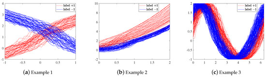
Figure 1. Samples of artificial numerical examples.

We perform a 10-fold cross-validation on these three artificial numerical examples to obtain the final experimental results and use the boxplot to denote the results, as shown in Figure 2. At the same time, we record the CPU time of two methods on the three datasets, as shown in Figure 3. It should be noted that the CPU time of the two methods is very different in Example 3, which leads to the time of FGEPSVM can hardly be seen when drawing the bar chart, so we have to deal with the time to some extent. We use $e^t$ instead of t, and t is the CPU time.

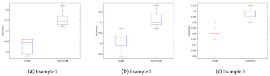
Figure 2. Boxplots of the results on artificial numerical examples.

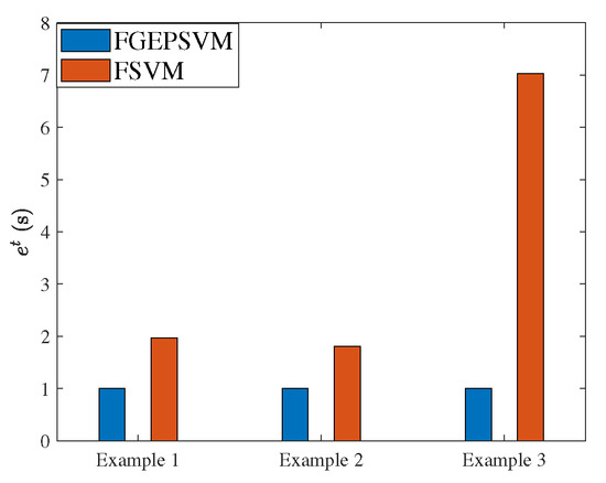
Figure 3. CPU time for two methods on artificial numerical examples.

We can see from Figure 2 that the results of the method in this paper are superior to FSVM on all three artificial datasets. The accuracy of FGEPSVM on the three artificial datasets are 0.7520, 0.7130 and 0.8985, respectively, while the corresponding results of FSVM are 0.6280, 0.6160 and 0.8780. Furthermore, our method is more stable on these three datasets. Figure 3 shows that our method has great advantages in terms of computation time. It is worth noting that nonparallel hyperplanes have certain advantages in dealing with crossed datasets. Therefore, we would like to explore whether the method proposed in this paper has the same advantages for crossed functional data in the functional space. The result of Example 1 illustrates this problem. The above artificial examples prove the feasibility and effectiveness of the proposed method.

4.2. Benchmark Datasets

We start with a detailed look at the six benchmark datasets. Coffee dataset is a two-class problem to distinguish between Robusta and Arabica coffee beans. ECG dataset contains the electrical activity recorded during one heartbeat and the two classes are a normal heartbeat and a Myocardial Infarction. Ham dataset includes measurements from Spanish and French dry-cured hams. The above three datasets are from the UCR time series classification and clustering website at http://www.cs.ucr.edu/~eamonn/time_series_data/ (accessed on 7 July 2020). Weather dataset consists of one year of daily temperature measurements from 35 Canadian weather stations, and the two classes are considered depending if the total yearly amount of precipitations are above or below 600 [3]. Growth dataset consists of 93 growth curves for a sample of 54 boys and 39 girls, and the observations were measured at a set of thirty-one ages from one to eighteen years old [3]. Tecator dataset consists of 215 near-infrared absorbance spectra of meat samples. Each observation consists of a 100-channel absorbance spectrum in the wavelength range 8,501,050 nm. The goal here is to predict whether the fat percentage is greater than 20% from the spectra. The dataset is available at http://lib.stat.cmu.edu/datasets/tecator (accessed on 1 January 2020). Table 1 shows the number of each dataset, dimension, and the functions of each class.

Table 1. Data description summary.

Datasets	Size	Dimension	Lable $+1$	Lable $-1$
weather	35	365	15	20
coffee	56	286	27	29
growth	93	31	54	39
ECG	200	96	133	67
ham	214	431	103	111
tecator	215	100	138	77

Samples of ten individuals of each dataset are plotted in Figure 4 ($d=0$), Figure 5 ($d=1$) and Figure 6 ($d=2$) are the first derivative and second derivative of the curves for functional datasets, respectively. The functional data in class $-1$ are plotted in solid blue line, whereas functional data in class $+1$ are depicted with a red dashed line.

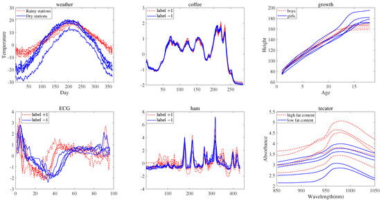
Figure 4. Original data for datasets ($d=0$).

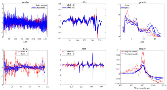
Figure 5. First derivative of the curves for datasets ($d=1$).

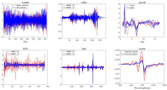
Figure 6. Second derivative of the curves for datasets ($d=2$).

We conduct experiments to evaluate the performance of FGEPSVM on six functional datasets. We record the averaged accuracy and CPU time on the testing set provided with the information given by the data ($d=0$), the first derivative ($d=1$), and the second derivative ($d=2$). Leave-one-out is performed on the weather, coffee, and growth datasets, whereas 10-fold cross-validation is implemented in ECG, ham, and tecator datasets. The classification results of the two methods are given in Table 2. The best classification accuracy of the two methods are highlighted in bold type.

Table 2. Accuracy results on functional datasets.

Dataset	d	FSVM	CPU Time (s)	FGEPSVM	CPU Time (s)
weather	0	0.8857	0.5911	0.8286	0.0018
	1	0.8286	0.8103	0.8000	0.0036
	2	0.6857	0.5692	0.9143	0.0156
coffee	0	0.9821	3.5711	0.9821	0.0031
	1	0.9464	1.3956	0.9464	0.0001
	2	0.7500	1.5059	0.7500	0.0056
growth	0	0.6882	4.8594	0.7634	0.0030
	1	0.9247	5.5469	0.9570	0.0025
	2	0.6667	5.0469	0.7634	0.0042
ECG	0	0.7280 ± 0.0127	2.1422	0.6840 ± 0.0084	0.0031
	1	0.6650 ± 0.0001	1.9187	0.6650 ± 0.0001	0.0031
	2	0.6680 ± 0.0035	2.0594	0.6660 ± 0.0120	0.0001
ham	0	0.6015 ± 0.0164	2.7484	0.6165 ± 0.0114	0.0031
	1	0.6033 ± 0.0203	3.7813	0.6139 ± 0.0179	0.0047
	2	0.5932 ± 0.0114	3.8891	0.6147 ± 0.0174	0.0016
tecator	0	0.8796 ± 0.0068	2.3344	0.8384 ± 0.0135	0.0001
	1	0.9902 ± 0.0033	2.3281	0.9196 ± 0.0055	0.0016
	2	0.9676 ± 0.0045	2.3031	0.9786 ± 0.0059	0.0016

In Table 2, FGEPSVM performed better than FSVM on most datasets. It is important to note that when the two methods produce the same results on the dataset, we consider our method more advantageous. This is based on computation time because we solve a pair of generalized eigenvalue problems, while the latter solves a quadratic programming problem. When dealing with the same dataset, the former calculation speed is significantly faster than the latter. Therefore, when the classification results are the same, we believe that FGEPSVM is more advantageous than FSVM. Furthermore, FSVM takes much more time than FGEPSVM on large-scale datasets, so that our approach has advantages in dealing with large-scale datasets.

Moreover, using higher-order derivative information also has a particular impact on classification performance. Higher-order derivative information can improve classification accuracy reflected in weather, growth, and tecator datasets. The classification accuracy of the second derivative for the weather dataset is much higher than that of the original function and the first derivative. Similarly, the classification results of the first derivative for the growth dataset are much higher than that of the original function and second derivative. Compared with the classification accuracy of the original function results, using the first derivative and the second derivative are improve the result for the tecator dataset. However, not all higher-order derivative information of datasets can do this. Therefore, when we solve functional data classification, we can appropriately consider using higher-order derivative information to improve the classification accuracy. In this paper, the first derivative and second derivative are considered in the numerical experiments. Any derivative can be used, which depends on the characteristics of the datasets.

We further apply the weighted linear combination of derivatives. The dimension of the weighted linear combination coefficient vector $\mathit{c}$ depends on how we use the d derivatives. This article uses the original function, the first derivative, and the second derivative, so $\mathit{c}$ is a three-dimensional vector. There are three weight coefficients, $c_0$, $c_1$, $c_2$. Since the sum of them is one, only two parameters are needed to select. Parameters $c_0$ and $c_1$ are selected from the values $\{0,\frac{1}{12},\dots ,\frac{11}{12},1\}$. One of the ways to select the optimal weighted linear combination coefficient vector is through k-fold cross-validation to obtain higher classification accuracy. Table 3 shows the classification results corresponding to the optimal parameters.

Table 3. Accuracy results on the weighted linear combination.

Dataset	c	FGEPSVM	CPU Time
weather	$\mathit{c}={(0,0,1)}^T$	0.9143	0.0156
coffee	$\mathit{c}={(\frac{1}{3},\frac{1}{2},\frac{1}{6})}^T$	1.0000	0.0001
growth	$\mathit{c}={(\frac{1}{3},0,\frac{2}{3})}^T$	0.9892	0.0001
ECG	$\mathit{c}={(\frac{11}{12},\frac{1}{12},0)}^T$	0.7005 ± 0.0169	0.0016
ham	$\mathit{c}={(\frac{1}{3},0,\frac{2}{3})}^T$	0.6326 ± 0.0232	0.0016
tecator	$\mathit{c}={(0,0,1)}^T$	0.9786 ± 0.0059	0.0016

In Table 3, the results in bold indicate that the classification results obtained by using weighted linear combination are better than those obtained by employing specific derivatives. The classification result of the original function on the coffee dataset is 0.9821, while the corresponding classification accuracy of the weighted linear combination is 1.0000. The classification accuracy corresponding to the first derivative on the growth dataset is 0.9570, while the classification accuracy is improved by 0.0322 after applying the weighted linear combination. Similarly, using the weighted linear combination of ham and ECG datasets also improves the accuracy compared to the previous results. Therefore, it also indicates that it is feasible and practical for us to consider employing the weight combination of derivatives.

4.3. Parameter Sensitivity Analysis

There is a key parameter $\delta$ in FGEPSVM. To analyze the sensitivity of the parameter, we study the effect of the parameter on classification accuracy. The parameter $\delta$ is selected from the values $\left\{{10}^i\right|i=-12,-11,\dots ,12\}$. For this study, we conduct experiments on datasets, as seen Figure 7.

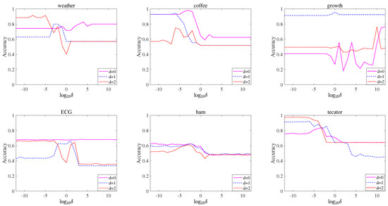
Figure 7. The classification performance of FGEPSVM with $\delta$ on datasets.

We find that FGEPSVM is sensitive to $\delta$. This indicates that $\delta$ has a greater impact on the performance of our proposal, so it needs to be adjusted carefully. It can also be seen that when the parameter $\delta$ is relatively small, the classification accuracy of most datasets is the best.

5. Conclusions

This paper proposes a functional generalized eigenvalue proximal support vector machine, which looks for two nonparallel hyperplanes in function space, making each functional hyperplane close to the functional data in one class and far away from the functional data in the other class. The corresponding optimization problem involves the inner product between two functional data, which can be replaced by the inner product between two coefficient vectors by introducing the orthonormal basis. Thus, the optimization problem in function space is transformed into the vector space through this orthonormal basis. Furthermore, our method is not restricted to the original functional data. The method presented in this paper can be applied to higher-order derivatives. Only when dealing with functional data can we consider using higher-order derivative information. We use the derivatives alone. Besides, we employ the weighted linear combination of derivatives that contain more information. It can be seen that the former is a particular case of the latter. We consider the weighted linear combination of the original function, first derivative, and second derivative. The results of numerical experiments show that the higher-order derivative information is critical to the performance of the classifier.

References

- Ramsay, J.O. When the data are functions. Psychometrika 1982, 47, 379–396. [Google Scholar] [CrossRef]
- Ramsay, J.O.; Dalzell, C.J. Some Tools for Functional Data Analysis. J. R. Stat. Soc. B 1991, 53, 539–572. [Google Scholar] [CrossRef]
- Ramsay, J.O.; Silverman, B.W. Functional Data Analysis; Springer: New York, NY, USA, 2005. [Google Scholar]
- Altland, H.W. Applied Functional Data Analysis. Technometrics 2003, 45, 101–102. [Google Scholar] [CrossRef]
- Auton, T. Applied Functional Data Analysis: Methods and Case Studies. J. R. Stat. Soc. A Stat. 2004, 167, 378–379. [Google Scholar] [CrossRef]
- Yao, F.; Muller, H.G.; Wang, J.L. Functional Data Analysis for Sparse Longitudinal Data. J. Am. Stat. Assoc. 2005, 100, 577–590. [Google Scholar] [CrossRef]
- Greenwood, M. Nonparametric Functional Data Analysis: Theory and Practice. J. R. Stat. Soc. A Stat. 2007, 102, 1077. [Google Scholar] [CrossRef]
- Aneiros, G.; Cao, R.; Fraiman, R.; Genest, C.; Vieu, P. Recent advances in functional data analysis and high-dimensional statistics. J. Multivar. Anal. 2018, 170, 3–9. [Google Scholar] [CrossRef]
- Ferraty, F.; Vieu, P. Curves discrimination: A nonparametric functional approach. Comput. Stat. Data Anal. 2003, 44, 161–173. [Google Scholar] [CrossRef]
- Ferraty, F. Most-predictive design points for functional data predictors. Biometrika 2010, 97, 807–824. [Google Scholar] [CrossRef]
- Leng, X.Y.; Müller, H.J. Classification using functional data analysis for temporal gene expression data. Bioinformatics 2006, 22, 68–76. [Google Scholar] [CrossRef]
- Lopez, M.; Martinez, J.; Matias, J.M.; Taboada, J.; Vilan, J.A. Functional classification of ornamental stone using machine learning techniques. J. Comput. Appl. Math. 2010, 234, 1338–1345. [Google Scholar] [CrossRef]
- Fortuna, F.; Battista, T.D. Functional unsupervised classification of spatial biodiversity. Ecol. Indic. 2020, 111, 106027. [Google Scholar] [CrossRef]
- Rossi, F.; Villa, N. Support vector machine for functional data classification. Neurocomputing 2005, 69, 730–742. [Google Scholar] [CrossRef]
- Li, B.; Yu, Q.Z. Classification of functional data: A segmentation approach. Comput. Stat. Data Anal. 2008, 52, 4790–4800. [Google Scholar] [CrossRef]
- Muñoz, A.; Gonzalez, J. Representing functional data using support vector machines. Pattern Recognit. Lett. 2009, 31, 511–516. [Google Scholar]
- Chang, C.; Chen, Y.K.; Todd Ogden, R. Functional data classification: A wavelet approach. Comput. Stat. 2014, 29, 1497–1513. [Google Scholar] [CrossRef]
- Martin-Barragan, B.; Lillo, R.; Romo, J. Interpretable support vector machines for functional data. Eur. J. Oper. Res. 2014, 232, 146–155. [Google Scholar] [CrossRef]
- Blanquero, R.; Carrizosa, E.; Jimenez-Cordero, A.; Martin-Barragan, B. Variable Selection in Classification for Multivariate Functional Data. Inf. Sci. 2018, 481, 445–462. [Google Scholar] [CrossRef]
- Berrendero, J.R.; Cuevas, A. Variable selection in functional data classification: A maxima-hunting proposal. Stat. Sin. 2016, 26, 619–638. [Google Scholar]
- Berrendero, J.R.; Cuevas, A.; Torrecilla, J.L. On the Use of Reproducing Kernel Hilbert Spaces in Functional Classification. J. Am. Stat. Assoc. 2018, 113, 1210–1218. [Google Scholar] [CrossRef]
- Blanquero, R.; Carrizosa, E.; Jimenez-Cordero, A.; Martin-Barragan, B. Functional-bandwidth Kernel for Support Vector Machine with Functional Data: An Alternating Optimization Algorithm. Eur. J. Oper. Res. 2018, 275, 195–207. [Google Scholar] [CrossRef]
- Vapnik, V.N. Statistical Learning Theory. Encycl. Sci. Learn. 1998, 41, 3185. [Google Scholar]
- Vapnik, V.N.; Lerner, A.Y. Recognition of Patterns with help of Generalized Portraits. Avtomat. U Telemekh 1963, 24, 774–780. [Google Scholar]
- Vapnik, V.N.; Chervonenkis, A.Y. A note on class of perceptron. Autom. Remote Control 1964, 25. Available online: http://www.kernel-machines.org/publications/VapChe64 (accessed on 10 April 2021).
- Boser, B.E.; Guyon, I.M.; Vapnik, V.N. A training algorithm for optimal margin classifiers. Comput. Learn. Theory 1992, 144–152. [Google Scholar] [CrossRef]
- Cortes, C.; Vapnik, V.N. Support-vector networks. Mach. Learn. 1995, 20, 273–297. [Google Scholar] [CrossRef]
- Jayadeva, R.K.; Khemchandani, R.; Chandra, S. Twin support vector machines for pattern classification. IEEE Trans. Pattern Anal. 2007, 29, 905–910. [Google Scholar] [CrossRef]
- Shao, Y.H.; Zhang, C.H.; Wang, X.B.; Deng, N.Y. Improvements on twin support vector machines. IEEE Trans. Neural. Netw. 2011, 22, 962–968. [Google Scholar] [CrossRef]
- Shao, Y.H.; Chen, W.J.; Deng, N.Y. Nonparallel hyperplane support vector machine for binary classification problems. Inf. Sci. 2014, 263, 22–35. [Google Scholar] [CrossRef]
- Tian, Y.J.; Qi, Z.Q.; Ju, X.C.; Shi, Y.; Liu, X.H. Nonparallel support vector machines for pattern classification. IEEE Trans. Cybern. 2014, 44, 1067–1079. [Google Scholar] [CrossRef] [PubMed]
- Mangasarian, O.L.; Wild, E.W. Multisurface proximal support vector machine classification via generalized eigenvalues. IEEE Trans. Pattern Anal. 2006, 28, 69–74. [Google Scholar] [CrossRef] [PubMed]
- Guarracino, M.R.; Cifarelli, C.; Seref, O.; Pardalos, P.M. A classification method based on generalized eigenvalue problems. Optim. Methods Softw. 2007, 22, 73–81. [Google Scholar] [CrossRef]
- Tikhonov, A.N.; Arsen, V.Y. Solutions of Ill-Posed Problems; Wiley: New York, NY, USA, 1977. [Google Scholar]
Publisher’s Note: MDPI stays neutral with regard to jurisdictional claims in published maps and institutional affiliations. |
© 2021 by the authors. Licensee MDPI, Basel, Switzerland. This article is an open access article distributed under the terms and conditions of the Creative Commons Attribution (CC BY) license (https://creativecommons.org/licenses/by/4.0/).