Copulaesque Versions of the Skew-Normal and Skew-Student Distributions

Abstract

A recent paper presents an extension of the skew-normal distribution which is a copula. Under this model, the standardized marginal distributions are standard normal. The copula itself depends on the familiar skewing construction based on the normal distribution function. This paper is concerned with two topics. First, the paper presents a number of extensions of the skew-normal copula. Notably these include a case in which the standardized marginal distributions are Student’s t, with different degrees of freedom allowed for each margin. In this case the skewing function need not be the distribution function for Student’s t, but can depend on certain of the special functions. Secondly, several multivariate versions of the skew-normal copula model are presented. The paper contains several illustrative examples.

1. Introduction

The recent paper by [1] presents an extension of the skew-normal distribution which has subsequently been referred to as a copula. Under this model, the standardized marginal distributions are standard normal and some of the conditional distributions are skew-normal.The skew-normal distribution itself was introduced in two landmark papers [2] and [3]. These papers have led to a very substantial research effort by numerous authors over the last thirty five years. The result of these efforts include, but are certainly not limited to, numerous probability distributions, both univariate and multivariate, which are loosely referred to in the literature as skew-elliptical distributions. This term does not completely describe the rich features of these distributions, but for convenience will be used in this paper. Notable contributions to these developments include papers by [4,5,6,7,8,9] among numerous others.

The many multivariate distributions that may be referred to as skew-elliptical offer coherent probability models that are used in a wide variety of applications. However, they all share the feature that the factor which perturbs symmetry is applied as a multiplier to a distribution that is elliptically symmetric. Consequently the marginal distributions are all prescribed. For example, the multivariate skew-t distribution described in [5] leads to marginal distributions that are all univariate skew-t distributions with the same degrees of freedom. While such a restriction may be acceptable or even irrelevant for some purposes, it is nonetheless the case that some multivariate applications have marginal distributions that are different. As is very well known, there is a large literature based on copulas which derives from the original paper of [10]. The purpose of a copula is to separate the modeling of the dependence structure of set of variables from the analysis of the marginal distributions. By implication, the marginal distributions need not be the same; that is, they may differ by more than just scale and location.

In a recent paper concerned primarily with projection pursuit, ref [1] presents a trivariate distribution based on the skew-normal which is also in a general sense a copula. The adjective general is used to refer to the fact that although the distribution does not satisfy the theoretical requirements laid down in [10] there is nonetheless separation between the modeling of the dependence structure and the treatment of the marginal distributions. The skew-normal and skew-Student copulas as they are termed in this paper are amenable to theoretical study, at least to some extent. Loperfido’s model also leads naturally to various extensions, which are of theoretical interest and which have the potential to provide tools for empirical research.

The purpose of this expository paper is to describe some of the properties of these new distributions and to present a number of extensions. As described below, these distributions are tractable to some extent, but numerous results of interest must be computed numerically. It is of particular interest to note that the some of the developments described in the paper are dependent on Meijer’s G function ([11]) and Fox’s H-function ([12]) and that there are therefore computational and methodological issues to be resolved. The structure of the paper is as follows: Section 2 summarizes a basic bivariate skew-normal copula and presents some of its properties. The bivariate model of this section is used to illustrate the difference from a bivariate normal copula that does satisfy the conditions of in [10]. Section 3 presents a conditional version of this distribution that has close connections to the original skew-normal distribution. Section 4 presents an extended version of the distribution; that is a distribution that is analogous to the extended skew-normal. Section 5 extends the results to an n-variate skew-normal copula and Section 6 to Student versions. This distribution in particular allows the marginal distributions to have different degrees of freedom. Section 7 presents results for a different multivariate setup. In this, a vector of $m+n$ variables may be partitioned into components of length m and n each of which has a marginal multivariate normal distribution. The properties of this distribution are briefly discussed, including an outline of a multivariate Student version. Section 8 presents three numerical examples. As this is an expository paper, several of the sections also contain brief discussions of technical issues that are outstanding and which could be the subject of future work. The final section of the paper contains a short summary.

Many of the results in this paper require numerical integration. Example results are generally computed to four decimal places. The usual notation $\varphi$ and $\mathrm{\Phi }$ are used to denote the standard normal density and distributions functions, respectively. To avoid proliferation of subscripts the notation $f\left(.\right)$ is used indifferently to denote a density function. Other notation, if not defined explicitly in the text, is that in common use.

2. The Skew-Normal Distribution as a Copula

The skew-normal copula was introduced by [1]. In their paper, the distribution is presented ariate form. Its principles may be demonstrated by a bivariate form of the distribution with probability density function

$$f\left(x_1,x_2\right)=2\varphi \left(x_1\right)\varphi \left(x_2\right)\mathrm{\Phi }\left(\lambda x_1{x}_2\right).$$

(1)

The scalar parameter $\lambda \in \mathbb{R}$ determines the extent of the dependence between $X_1$ and $X_2$. In Section 5, the bivariate distribution is extended to n variables. To accommodate this extension it is convenient to employ the notation $\mathbf{X}\sim SN{C}_n\left(\lambda \right)$, where $\mathbf{X}={\left(X_1,X_2,\cdots ,X_n\right)}^{\mathit{T}}$. As [1] shows, in the bivariate case the marginal distribution of each $X_i$ is $N\left(0,1\right)$ and the conditional distribution of $X_1$ given that $X_2=x_2$ is skew-normal with density function

$$f\left(x_1|X_2=x_2\right)=2\varphi \left(x_1\right)\mathrm{\Phi }\left(\lambda x_1{x}_2\right).$$

(2)

There is an analogous expression for the density function of the conditional distributions of $X_2$ given that $X_1=x_1$. It may also be noted that $X_2^2$ is distributed independently of $X_1$ as a ${\chi }_{\left(1\right)}^2$ variable, with the analogous result for the distributions of $X_2$ and $X_1^2$. Hence the $X_i^2$, $i=1,2$ are independently distributed as ${\chi }_{\left(1\right)}^2$.

To illustrate the difference from the formal definition of a copula, consider the well-known Gaussian copula. In the bivariate case, dependence between $X_1$ and $X_2$ is described by the function

$${\mathrm{\Phi }}_{2,\mathit{C}}\left\{{\mathrm{\Phi }}^{-1}\left(U_1\right),{\mathrm{\Phi }}^{-1}\left(U_2\right)\right\},$$

where ${\mathrm{\Phi }}_{2,\mathit{C}}\left\{..\right\}$ denotes the distribution function of a bivariate normal distribution with zero means and correlation matrix $\mathit{C}$ and the $U_{1,2}$ are each uniformly distributed on $\left[0,1\right]$. The formulation at Equation (2) uses only the standard univariate normal distribution function.

Sketches of the skew-normal density function for $\lambda \in \left\{-10.0,-2.6,0.0,10.0\right\}$ are shown in Figure 1. Sketches of the bivariate density function for $\lambda =1.0$ and $-5.0$ are shown in Figure 2. The bi-modal nature of the density function when $\lambda =-5.0$ is noteworthy. Indeed it is straight forward to show that the density function is bi-modal if $\left|\lambda \right|>\sqrt{\pi /2}$, with the model values being at points $\pm \left(X,X\right)$ depending on $\lambda$. Examples of modal values are shown in Table 1 for a range of values of $\lambda$.

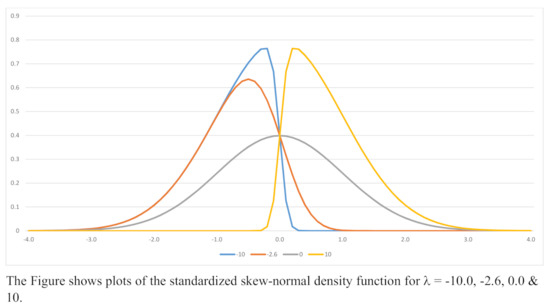
Figure 1. Skew-normal Density Functions; $\lambda =-10.0,-2.6,0.0,10.0$.

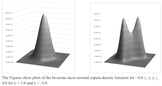
Figure 2. Bivariate Skew-normal Copula Density Functions; $\lambda =1.0,-5.0$.

Table 1. Modal Values of the Bivariate Skew-normal Copula Distribution.

$\mathit{\lambda }$	Mode	$\mathit{\lambda }$	Mode
1.254	0.0231	35	0.2564
1.275	0.1296	50	0.2213
3	0.5422	75	0.1865
4	0.5258	10${}^3$	0.1648
5	0.5029	10${}^3$	0.0588
15	0.3565	10${}^4$	0.0200
10	0.4112	10${}^5$	0.0063
20	0.3299	10${}^6$	0.0020

Cross-Moments

The covariance of $X_1$ and $X_2$, which also equals their correlation, is

$$cov\left(X_1,X_2\right)=2{\int }_{-\infty }^{\infty }{\int }_{-\infty }^{\infty }{x}_1{x}_2\varphi \left(x_1\right)\varphi \left(x_2\right)\mathrm{\Phi }\left(\lambda x_1{x}_2\right)d{x}_{1}d{x}_2,$$

(3)

which is readily shown to be

$$cov\left(X_1,X_2\right)=2\left(\lambda /\sqrt{2\pi }\right){\int }_{-\infty }^{\infty }\left(x_2^2/\sqrt{1+{\lambda }^2{x}_2^2}\right)\varphi \left(x_2\right)d{x}_2,$$

(4)

or

$$cov\left(X_1,X_2\right)=\left(\lambda \sqrt{2/\pi }\right){\int }_0^{\infty }\left(y/\sqrt{1+{\lambda }^{2}y}\right)f\left(y\right)dy,$$

(5)

where $Y\sim {\chi }_{\left(1\right)}^2$. There is no reported analytic expression for this integral in general. However, it equals zero when $\lambda =0$ and tends to $\pm 2/\pi$ as $\lambda \to \pm \infty$. Note that the integral in Equation (5) may also be expressed in terms of a Chi-squared distribution with 3 degrees of freedom. Table 2 shows values of the correlation for a range of positive values of $\lambda$.

Table 2. Correlation of the Bivariate Skew-normal Copula Distribution.

$\mathit{\lambda }$	Cov(=Cor)	$\mathit{\lambda }$	Cov(=Cor)
0.0010	0.0008	0.5000	0.3129
0.0020	0.0016	1.0000	0.4505
0.0040	0.0032	2.0000	0.5503
0.0100	0.0080	5.0000	0.6116
0.0200	0.0159	10.0000	0.6268
0.0500	0.0397	20.0000	0.6316
0.1000	0.0786	50.0000	0.6331
0.2000	0.1511	100.0000	0.6333

For higher order cross-moments the following results hold. If p and q are positive integers with $p+q$ odd, then

$$E\left(X_1^p{X}_2^q\right)=0.$$

(6)

Note that there is no need to derive this result using integration by parts. Since p or q must be even, it is a consequence of one of the properties above, as is the result for the case where p and q are both even

$$E\left(X_1^p{X}_2^q\right)=2^{\frac{p+q}{2}}\mathrm{\Gamma }\left(\frac{p+1}{2}\right)\mathrm{\Gamma }\left(\frac{q+1}{2}\right)/\pi .$$

(7)

For p and q both odd, the expectation satisfies the recursion

$$E\left(X_1^p{X}_2^q\right)=\left(p-1\right)E\left(X_1^{p-2}{X}_2^q\right)+\lambda \sqrt{\left(2/\pi \right)}{\int }_{-\infty }^{\infty }\left\{x^{q+1}/{\left(1+{\lambda }^2{x}^2\right)}^{p/2}\right\}\varphi \left(x\right)dx,$$

(8)

with

$$E\left(X_1{X}_2^q\right)=\lambda \sqrt{\left(2/\pi \right)}{\int }_{-\infty }^{\infty }\left\{x^{q+1}/{\left(1+{\lambda }^2{x}^2\right)}^{1/2}\right\}\varphi \left(x\right)dx.$$

(9)

In a recent paper, ref [13] show that cross-moments of this distribution may also be computed using a new extension of Stein’s lemma, ref [14]. There is no particular advantage in using the new lemma for the bivariate distribution at Equation (1). The result is however employed in Section 5 which is concerned with the more general case of n variables. If $p=2k+1$ and $q=2l+1$, it is straightforward to show that as $\lambda \to \pm \infty$ the limiting value of $E\left(X^p{Y}^q\right)$ is

$$li{m}_{\lambda \to \infty }E\left(X^p{Y}^q\right)=\pm 2^{k+l+1}k!l!/\pi .$$

The limiting values of a selection of odd order cross moments $E\left(X_1^p{X}_2^q\right)$ are shown in Table 3 and a selection of moments corresponding to $\lambda =1.0$ in Table 4.

Table 3. Cross Moments—Limiting Values.

Order	1	3	5	7	9
1	0.6366	1.2732	5.093	30.5577	244.462
3		2.5481	10.1891	61.1282	489.0004
5			40.7564	244.5129	1956.0016
7				1467.0776	11,736.0093
9					93,888.0744

Table 4. Cross Moments: $\lambda =1.0$.

Order	1	3	5	7	9
1	0.4507	1.0808	4.5040	27.4555	221.5542
3	1.0808	2.4329	9.9094	59.7483	478.9353
5	4.5040	9.9094	40.1754	241.9398	1938.3608
7	27.4555	59.7483	241.9398	1456.7783	11,670.9677
9	221.5542	478.9353	1938.3608	11,670.9677	93,501.497
11	2227.8507	4794.0952	19,397.487	116,791.7771	935,671.459
13	26,837.3188	57,561.2949	232,862.2301	1,402,049.0507	11,232,438.0284

Although not specifically required for the determination of the normalization constant in Equation (1), the distribution of the product $Y=X_1{X}_2$ for the case where each $X_i,i=1,2$ is independently distributed as $N\left(0,1\right)$ is of interest. When $X_i\sim N\left(0,{\sigma }_i^2\right)$ independently for $i=1,2$, the distribution of Y has the density function

$$f\left(y\right)=K_0\left(\left|y\right|/{\sigma }_1{\sigma }_2\right)/\pi {\sigma }_1{\sigma }_2,$$

(10)

where $K_0\left(.\right)$ is the modified Bessel function of the second kind. See, for example, ref [15] for further details of this result and [16] (Chapter 9, Sections 6 to 8) for details of the function K itself.

3. A New Skew-Normal Type Distribution

As noted above in Section 2, the conditional distribution of $X_1$ given $X_2=x_2$ is skew-normal with shape parameter $\lambda x_2$. A new univariate distribution may be obtained by conditioning instead on $X_2\le y$. The resulting distribution of $X_1$ has the density function

$$f\left(x\right)=2\varphi \left(x\right)\left\{{\int }_{-\infty }^y\varphi \left(s\right)\mathrm{\Phi }\left(\lambda xs\right)ds\right\}/\mathrm{\Phi }\left(y\right).$$

(11)

Straight forward integration gives the following results.

Proposition 1.

Let X have the distribution with density function given by Equation (11). The following results hold:

1.

An alternative expression for the density function is

$$f\left(x\right)=2\varphi \left(x\right)\mathrm{\Phi }\left(\lambda yx\right)-2\lambda x\varphi \left(x\right)\left\{{\int }_{-\infty }^y\mathrm{\Phi }\left(s\right)\mathrm{\varphi }\left(\lambda xs\right)ds\right\}/\mathrm{\Phi }\left(y\right).$$

(12)

2.

A second alternative expression is

$$f\left(x\right)=\varphi \left(x\right)-2x\varphi \left(x\right){\xi }_1\left(y\right){\int }_0^{\lambda }\frac{\varphi \left(\lambda xy\right)}{1+{\lambda }^2{x}^2}d\lambda ,$$

(13)

where ${\xi }_1\left(x\right)=\varphi \left(x\right)/\mathrm{\Phi }\left(x\right)$.

3.

$X^2$ is distributed as ${\chi }_{\left(1\right)}^2$.

4.

Odd order moments may be computed recursively from

$$E\left(X^n\right)=\left(n-1\right)E\left(X^{n-2}\right)+\sqrt{2/\pi }\lambda \left\{E\left(Z^{n-1}\right)/\mathrm{\Phi }\left(y\right)\right\}{\int }_{-\infty }^y\frac{s\varphi \left(s\right)}{{\left(1+{\lambda }^2{s}^2\right)}^{n/2}}ds,$$

(14)

with $Z\sim N\left(0,1\right)$ and

$$E\left(X\right)=\left\{\sqrt{2/\pi }\lambda /\mathrm{\Phi }\left(y\right)\right\}{\int }_{-\infty }^y\frac{s\varphi \left(s\right)}{{\left(1+{\lambda }^2{s}^2\right)}^{1/2}}ds.$$

(15)

The expression at Equation (13) may be computed using the methods reported in [17]. This distribution possesses two interesting properties as $\left|y\right|\to \infty$.

Proposition 2.

Let X have the distribution with density function given by Equation (11). The following results hold:

1.

For $\lambda >0$, as $y\to -\infty$ the limiting form of the distribution of X is skew-normal with shape parameter $\lambda y$; that is

$$li{m}_{y\to -\infty }f\left(x\right)=2\varphi \left(x\right)\mathrm{\Phi }\left(\lambda yx\right).$$

(16)

2.

For $\lambda >0$ as $y\to \infty$

$$li{m}_{y\to \infty }f\left(x\right)=\varphi \left(x\right).$$

(17)

Part 1 of the proposition may be established using the well-known asymptotic formula for the standard normal integral ([16], page 932, Equation 26.2.12); that is

$$\mathrm{\Phi }\left(x\right)\simeq \varphi \left(x\right)/\left|x\right|;x<<0,$$

(18)

and integration by parts. In this case for $\lambda >0$ and $y<<0$ the second term is negligible. There are analogous results for $\lambda <0$. Equation (18) and the same assumption are used again in some of the results below. It is interesting to note that Part 1 of the propsition results in the same density function as that at Equation (2).

Numerical computations or asymptotic arguments are necessary in order to employ the distribution at Equation (11); for example to compute moments or critical values. Nonetheless, it is arguably a more flexible form than the familiar skew-normal shown at Equation (2). Examples of the density functions from Equations (2) and (11) are shown in Figure 3. In Table 5, $m1$ and $m3$ are the first and third moment about the origin, $sk$ and $ku$ are skewness and kurtosis, $ssk$ and $sku$ are the corresponding standardized values. The table shows a selection of moments for $\lambda =1$ and a range of values of y from $-10.0$ to $10.0$. For positive values of y, skewness and kurtosis rapidly tend to 0 and 3 , respectively. For $y<0$ skewness is negative and there is excess kurtosis. As above, there are analogous results for $\lambda <0$.

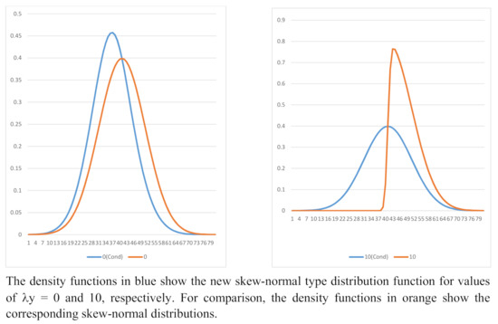
Figure 3. Comparison of the Skew-normal and New Skew-normal Type Distributions; $\lambda y=0.0$ and $10.0$.

Table 5. Moments of New Skew-normal Type Distribution Function; $\lambda =1$.

$\le \mathit{y}$	$\mathit{m}1$	$\mathit{m}3$	$\mathit{sk}$	$\mathit{ssk}$	$\mathit{ku}$	$\mathit{sku}$
−10.0	−0.7940	−1.5957	−0.2148	−0.9563	0.5223	3.8241
−7.6	−0.7913	−1.5956	−0.2126	−0.9302	0.5304	3.7942
−5.1	−0.7839	−1.5950	−0.2068	−0.8640	0.5527	3.7198
−2.6	−0.7538	−1.5884	−0.1836	−0.6471	0.6514	3.4929
0.0	−0.4174	−1.0540	0.0528	0.0703	2.1945	3.2182
2.4	−0.0062	−0.0131	0.0054	0.0054	2.9999	3.0001
4.9	0.0000	0.0000	0.0000	0.0000	3.0000	3.0000
7.4	0.0000	0.0000	0.0000	0.0000	3.0000	3.0000
10.0	0.0000	0.0000	0.0000	0.0000	3.0000	3.0000

4. An Extended Skew-Normal Copula

The skew-normal and skew-Student distributions have extended forms. These arise naturally when conditional distributions are considered. They also arise as hidden truncation models. In standardized form, the univariate extended skew-normal distribution has the density function

$$f\left(x\right)=\varphi \left(x\right)\mathrm{\Phi }\left(\tau \sqrt{1+{\lambda }^2}+\lambda x\right)/\mathrm{\Phi }\left(\tau \right);\tau \in \mathbb{R}.$$

(19)

The extended skew-normal distribution may be derived by considering a standardized bivariate normal distribution of X and Y with correlation $\rho$. The distribution at Equation (19) is the density of X given that $Y\ge -\tau$, with $\lambda =\rho /\sqrt{1-{\rho }^2}$. The distribution may be denoted $ESN\left(\lambda ,\tau \right)$. A bivariate extended skew-normal copula distribution that is analogous to that in Section 2 has the density function

$$f\left(x_1,x_2\right)=\varphi \left(x_1\right)\varphi \left(x_2\right)\mathrm{\Phi }\left(\tau \sqrt{1+{\lambda }^2}+\lambda x_1{x}_2\right)/\Omega \left(\tau ,\lambda \right),$$

(20)

where $\Omega \left(\tau ,\lambda \right)>0$ is the normalizing constant. Integration with respect to $X_1$ shows that

$$\Omega \left(\tau ,\lambda \right)={\int }_{-\infty }^{\infty }\varphi \left(y\right)\mathrm{\Phi }\left(\tau \sqrt{1+{\lambda }^2}/\sqrt{1+{\lambda }^2{y}^2}\right)dy,$$

(21)

which may be evaluated numerically. In addition, the marginal distribution of X is symmetric and has the density function.

$$f\left(x\right)=\varphi \left(x\right)\mathrm{\Phi }\left(\tau \sqrt{1+{\lambda }^2}/\sqrt{1+{\lambda }^2{x}^2}\right)/\Omega \left(\tau ,\lambda \right).$$

(22)

Values of $\Omega \left(\tau ,\lambda \right)$ computed to four decimal places for a selection of values of $\tau$ and $\lambda$ are shown in Table 6. Note that for values of $\tau$ less than say $-5$ the values of $\Omega$ are small, implying the need for care with its computation. The shorthand notation $\mathbf{X}\sim ESN{C}_n\left(\tau ,\lambda \right)$ which extends that defined in Section 2 will be used. The basic properties of the bivariate extended skew-normal copula distribution are as follows.

Table 6. Normalising Constant for the ESNC Distribution.

$\mathit{\tau }/\mathit{\lambda }$	0.5	1	2.5	5	10	25
−15	0.0000	0.0000	0.0000	0.0000	0.0000	0.0000
−10	0.0000	0.0000	0.0000	0.0000	0.0000	0.0000
−5	0.0000	0.0002	0.0008	0.001	0.0011	0.0011
−2.5	0.0072	0.0105	0.0155	0.0168	0.0172	0.0173
−1	0.1550	0.1396	0.1108	0.1057	0.1048	0.1045
−0.5	0.3051	0.2898	0.2412	0.2138	0.2069	0.2052
0	0.5000	0.5000	0.5000	0.5000	0.5000	0.5000
0.5	0.6949	0.7102	0.7588	0.7862	0.7931	0.7948
1	0.8450	0.8604	0.8892	0.8943	0.8952	0.8955
2.5	0.9928	0.9895	0.9845	0.9832	0.9828	0.9827
5	1.0000	0.9998	0.9992	0.999	0.9989	0.9989
10	1.0000	1.0000	1.0000	1.0000	1.0000	1.0000
15	1.0000	1.0000	1.0000	1.0000	1.0000	1.0000

Proposition 3.

Let ${\left(X_1,X_2\right)}^{\mathit{T}}\sim ESN{C}_2\left(\tau ,\lambda \right)$, let X denote either variable and define

$${\tilde{\tau }}_x=\frac{\tau \sqrt{1+{\lambda }^2}}{\sqrt{1+{\lambda }^2{x}^2}}.$$

(23)

The following properties hold

1. $E\left(X\right)=0$.

2. $var\left(X\right)=1-\left\{{\lambda }^2\tau \sqrt{1+{\lambda }^2}/\Omega \left(\tau ,\lambda \right)\right\}{\int }_{-\infty }^{\infty }\frac{y^2}{{\left(1+{\lambda }^2{y}^2\right)}^{3/2}}\varphi \left({\tilde{\tau }}_y\right)\varphi \left(y\right)dy$.

3. $cov\left(X_1,X_2\right)=\left\{\lambda /\Omega \left(\tau ,\lambda \right)\right\}{\int }_{-\infty }^{\infty }\frac{y^2}{\sqrt{1+{\lambda }^2{y}^2}}\varphi \left({\tilde{\tau }}_y\right)\varphi \left(y\right)dy$.

4. $X_1|X_2=y\sim ESN\left({\tilde{\tau }}_y,\lambda y\right)$.

Proof of this proposition is in the Appendix A. Table 7 shows standard errors for a range of values of $\tau$ and $\lambda$. These were computed using numerical integration. Table 8 shows the correlation coefficients for a range of parameter values. For $\lambda =1.0$ Figure 4 shows (i) an example of the bivariate skew-normal density function for $\tau =-1.0$ and (ii) the marginal density for $\tau =-2.5$ and $0.0$. Higher order cross moments may be computed recursively, but for non-zero values of $\tau$ the resulting integrals are two-dimensional. Depending on the values of $\lambda$ and $\tau$ the extended version of the distribution is also bi-modal.

Table 7. Standard Errors for the ESNC Distribution.

$\mathit{\tau }/\mathit{\lambda }$	0.5	1	2.5	5	10	25
−15	5.563804	4.654258	4.178148	4.089074	4.065563	4.058883
−10	4.441411	3.816603	3.472084	3.40682	3.38956	3.384654
−5	2.886818	2.724329	2.574579	2.54366	2.535375	2.533012
−2.5	1.610455	1.924303	1.967713	1.966597	1.965964	1.96576
−1	1.113491	1.249359	1.453953	1.498411	1.507775	1.510312
−0.5	1.041259	1.092314	1.208643	1.283663	1.304663	1.309794
0	1.000000	1.000000	1.000000	1.000000	1.000000	1.000000
0.5	0.981337	0.95979	0.923856	0.907661	0.903814	0.902917
1	0.977757	0.953395	0.927976	0.923458	0.922466	0.922193
2.5	0.994202	0.985502	0.977147	0.975165	0.974617	0.974459
5	0.999946	0.999327	0.997783	0.997263	0.997109	0.997064
10	1.000000	0.999999	0.999985	0.999976	0.999973	0.999972
15	1.000000	1.000000	1.000000	1.000000	1.000000	1.000000

Table 8. Correlation for the ESNC Distribution.

$\mathit{\tau }/\mathit{\lambda }$	0.5	1	2.5	5
−15	0.9840	0.9772	0.9718	0.9705
−10	0.9750	0.9662	0.9594	0.9578
−5	0.9419	0.9348	0.9273	0.9256
−2.5	0.8174	0.8745	0.8788	0.8786
−1	0.5440	0.7087	0.7914	0.8007
−0.5	0.4272	0.5909	0.7154	0.7417
0	0.3130	0.4507	0.5721	0.6125
0.5	0.2112	0.3122	0.3892	0.4034
1	0.1294	0.1975	0.2422	0.2492
2.5	0.0156	0.0355	0.0561	0.0611
5	0.0001	0.0015	0.0049	0.0060
10	0.0000	0.0000	0.0000	0.0001
15	0.0000	0.0000	0.0000	0.0000

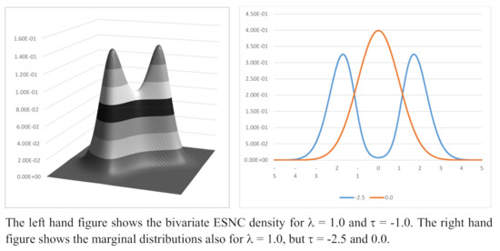
Figure 4. Extended Skew-normal Copula Density Functions; $\lambda =1.0$.

The extended version of the distribution has a conditional distribution that is similar to that described in Proposition 2. As above, proof is in the Appendix A.

Proposition 4.

Let $X_1$ and $X_2$ have the distribution with density function given by Equation (20). The following results hold:

1.

The normalizing constant $\Omega \left(\tau ,\lambda \right)$ is given by

$$\Omega \left(\tau ,\lambda \right)=1/2+\tau {\lambda }^2\sqrt{1+{\lambda }^2}{\int }_{-\infty }^{\infty }\frac{y\mathrm{\Phi }\left(y\right)\varphi \left({\tilde{\tau }}_y\right)}{{\left(1+{\lambda }^2{y}^2\right)}^{3/2}}dy.$$

(24)

2.

The distribution function of $X_2$ is

$$Pr\left(X_2\le y\right)={\int }_{-\infty }^y\varphi \left(s\right)\mathrm{\Phi }\left(\tau \sqrt{1+{\lambda }^2}/\sqrt{1+{\lambda }^2{s}^2}\right)ds/\Omega \left(\tau ,\lambda \right).$$

(25)

3.

The density function of $X_1$ given that $X_2\le y$ is

$$f\left(x_1|X_2\le y\right)=\varphi \left(x_1\right)\frac{{\int }_{-\infty }^y\varphi \left(s\right)\mathrm{\Phi }\left(\tau \sqrt{1+{\lambda }^2}+\lambda x_{1}s\right)ds}{{\int }_{-\infty }^y\varphi \left(s\right)\mathrm{\Phi }\left(\tau \sqrt{1+{\lambda }^2}/\sqrt{1+{\lambda }^2{s}^2}\right)ds}$$

(26)

4.

For $\lambda >0$, as $y\to -\infty$ the limiting form of the distribution of $X_1$ has the density function

$$li{m}_{y\to -\infty }f\left(x_1\right)=\varphi \left(x_1\right)\mathrm{\Phi }\left({\tilde{\tau }}_y\sqrt{1+{\tilde{\lambda }}_y^2}+{\tilde{\lambda }}_y{x}_1\right)/\mathrm{\Phi }\left({\tilde{\tau }}_y\right),$$

(27)

where ${\tilde{\tau }}_y$ is as defined in Proposition 3 and ${\tilde{\lambda }}_y=\lambda y$; that is, $X_1|X_2\le y\sim ESN\left({\tilde{\tau }}_y,\lambda y\right)$.

4.

Note that as in Section 3 the distributions in Part 4 of both Propositions 3 and 4 are the same. There are analogous results for $\lambda <0$ as $y\to \infty$.

5. Extension to $\mathbf{n}$ Variables

There is a self-evident extension for the distribution of an n-vector $\mathbf{X}$, with i-$th$ element $X_i$, which has density function

$$f\left(\mathbf{x}\right)=2{\mathrm{\Pi }}_{i=1}^n\varphi \left(x_i\right)\mathrm{\Phi }\left(\lambda {\mathrm{\Pi }}_{i=1}^n{x}_i\right),$$

(28)

and shorthand notation $\mathbf{X}\sim SN{C}_n\left(\lambda \right)$. Recall that [1] describes the case $n=3$. This distribution has the following properties:

• The marginal distribution of each $X_i$ is $N\left(0,1\right)$.
• The members of any subset of $\mathbf{X}$ of size 2,…, $n-1$ are independently distributed as $N\left(0,1\right)$.
• The $X_i^2$; $i=1,\dots ,n$ are independently distributed at ${\chi }_{\left(1\right)}^2$ variables.
• If $\mathbf{X}$ is partitioned into two non-overlapping sets, $\left\{X_i\right\};i=1,\dots ,p$ and $\left\{X_j\right\};j=p+1,\dots ,p+q$ with $p+q\le n$ then (i) the $\left\{X_i^2\right\}$ are independently distributed as ${\chi }_{\left(1\right)}^2$ variables independently of (ii) the $\left\{X_j\right\}$, which are themselves independently distributed as $N\left(0,1\right)$.
• The distribution of $X_i$ given $X_j=x_j,j\ne i$ is skew-normal, with density function

  $$f\left(x_i\right)=2\varphi \left(x_i\right)\mathrm{\Phi }\left(\lambda {\mathrm{\Pi }}_{i=1}^n{x}_i\right),$$

  (29)

  that is, with shape parameter $\lambda {\mathrm{\Pi }}_{j\ne i}^n{x}_j$.
• The distribution of $X_j,j\ne i$ given $X_i=x_i$ is a skew-normal copula, with shape parameter $\lambda x_i$.

Other properties are briefly described in the rest of this section.

5.1. Cross-Moments

The first order cross-moment is

$$E\left({\mathrm{\Pi }}_{i=1}^n{X}_i\right)=\lambda \sqrt{2/\pi }{\int }_{-\infty }^{\infty }\cdots {\int }_{-\infty }^{\infty }\left({\mathrm{\Pi }}_{i=1}^{n-1}{x}_i^2\varphi \left(x_i\right)/\sqrt{1+{\lambda }^2{\mathrm{\Pi }}_{i=1}^{n-1}{x}_i^2}\right){\mathrm{\Pi }}_{i=1}^{n-1}\left(d{x}_i\right).$$

(30)

As $\left|\lambda \right|$ increases the limiting value of Equation (30) is $\pm {\left(2/\pi \right)}^{n/2}$. There are expressions for higher order multivariate moments which are similar to those at Equations (7) and (8). If the $\left\{p_i\right\};i=1,\cdots ,n$ are all even then property (4) implies that

$$E\left({\mathrm{\Pi }}_{i=1}^n{X}_i^{p_i}\right)={\mathrm{\Pi }}_{i=1}^n\Gamma \left(\frac{p_i+1}{2}\right)/2^{P/2}\Gamma {\left(1/2\right)}^n;P={{\Sigma }}_{i=1}^n{p}_i.$$

(31)

If any $p_i$ is even and any other is odd then the expectation at the left hand side of Equation (31) is zero. For the general multivariate case with all $\left\{p_i\right\}$ odd , higher order cross-moments may be computed in principle using a version of the extension to Stein’s lemma reported in [13], as follows:

Proposition 5.

Extension to Stein’s lemma ([13])

Let ${\mathbf{X}}^{\mathit{T}}=\left(X_1,X_2,\cdots ,X_n\right)$ and let $g\left(\mathbf{X}\right):{\mathbb{R}}^n\to \mathbb{R}$ be a function that is differentiable almost everywhere. Noting that

$${\mathrm{\Pi }}_{i=1}^n\varphi \left(x_i\right)={\varphi }_n\left(\mathbf{x}\right),$$

is the density function of the standard multivariate normal distribution evaluated at $\mathbf{X}=\mathbf{x}$, the extension to Stein’s lemma states that

$$cov\left\{\mathbf{X},g\left(\mathbf{X}\right)\right\}=E\left\{\nabla g\left(\mathbf{X}\right)\right\}+2{\int }_{-\infty }^{\infty }\cdots {\int }_{-\infty }^{\infty }g\left(\mathbf{x}\right)\nabla \mathrm{\Phi }\left(\lambda {\mathrm{\Pi }}_{i=1}^n{x}_i\right)\varphi \left(\mathbf{x}\right)d\mathbf{x},$$

where E denotes expectation taken over the skew-normal copula density function at Equation (28).

The gradient vector of $\mathrm{\Phi }\left(\lambda {\mathrm{\Pi }}_{i=1}^n{x}_i\right)$ is

$$\nabla \mathrm{\Phi }\left(\lambda {\mathrm{\Pi }}_{i=1}^n{x}_i\right)=\lambda \left[\begin{array}{c}{\mathrm{\Pi }}_{j=2}^n{X}_j\\ ⋮\\ {\mathrm{\Pi }}_{j\ne i}{X}_j\\ ⋮\\ {\mathrm{\Pi }}_{j=1}^{n-1}{X}_j\end{array}\right]\varphi \left(\lambda {\mathrm{\Pi }}_{i=1}^n{x}_i\right).$$

(32)

When

$$g\left(\mathbf{X}\right)=X_1^{(p_1-1)}{\mathrm{\Pi }}_{i=2}^n{X}_i^{p_i};p_i\in {\mathbb{I}}^{+},$$

(33)

$\nabla g$ is given by

$$\nabla g\left(\mathbf{X}\right)=\left[\begin{array}{c}(p_1-1)X_1^{p_1-2}{\mathrm{\Pi }}_{j=2}^n{X}_j^{p_j}\\ ⋮\\ p_i{X}_1^{p_1-1}{X}_i^{p_i-1}{\mathrm{\Pi }}_{j\ne 1,i}{X}_j^{p_j}\\ ⋮\\ p_n{X}_1^{p_1-1}{X}_n^{p_n-1}{\mathrm{\Pi }}_{j=2}^{n-1}{X}_j^{p_j}\end{array}\right].$$

(34)

The first term of the vector $cov\left\{\mathbf{X},g\left(\mathbf{X}\right)\right\}$ recovers $E\left({\mathrm{\Pi }}_{i=1}^n{X}_i^{p_i}\right)$. Use of the lemma in Proposition 5 shows that

$$\begin{array}{cc}\hfill E\left({\mathrm{\Pi }}_{i=1}^n{X}_i^{p_i}\right)& =\hspace{1em}\left(p_1-1\right)E\left(X_1^{p_1-2}{\mathrm{\Pi }}_{i=2}^n{X}_i^{p_i}\right)+\hfill \\ \hfill & 2\lambda {\int }_{-\infty }^{\infty }\cdots {\int }_{-\infty }^{\infty }{x}_1^{p_1-1}{\mathrm{\Pi }}_{i=2}^n{x}_i^{p_i+1}{\mathrm{\Pi }}_{i=1}^n\left\{\varphi \left(x_i\right)\right\}\varphi \left(\lambda {\mathrm{\Pi }}_{i=1}^n{x}_i\right)d\mathbf{x}.\hfill \end{array}$$

(35)

Note that the second term is equal to zero if $p_1$ is even. Otherwise it may be reduced to an integral in $n-1$ dimensions

$$\sqrt{\frac{2}{\pi }}\lambda {\alpha }_{p_1-1}{\int }_0^{\infty }\cdots {\int }_0^{\infty }\frac{{\mathrm{\Pi }}_{i=2}^n{y}_i^{\left(p_i+1\right)/2}}{{\left(1+{\lambda }^2{\mathrm{\Pi }}_{i=2}^n{y}_i\right)}^{p_1/2}}{\mathrm{\Pi }}_{i=2}^{n}f\left(y_i\right)d\mathbf{x}$$

with

$${\alpha }_{p_1-1}=\Gamma \left(p_1/2\right)2^{\left(p_1-1\right)/2}/\Gamma \left(1/2\right),$$

and the variables $Y_i$ each independently distributed as ${\chi }_{\left(1\right)}^2$.

Note that the second and subsequent elements of $cov\left\{\mathbf{X},g\left(\mathbf{X}\right)\right\}$ will recover other cross-moments.

5.2. Skew Distributions Generated by Conditioning

Similar to the results in Section 3 a skewed distribution may be obtained by conditioning on $X_1\le y$. The distribution has the density function

$$f\left(x_i;i=2,\cdots ,n|X_1\le y\right)={\mathrm{\Pi }}_{i=2}^n\varphi \left(x_i\right){\int }_{-\infty }^y\varphi \left(s\right)\mathrm{\Phi }\left(\lambda s{\mathrm{\Pi }}_{i=2}^n{x}_i\right)ds/\mathrm{\Phi }\left(y\right).$$

(36)

Using arguments similar to those in Section 3, it then follows that for $\lambda >0$ and as $y\to -\infty$ the distribution of the $n-1$ vector $\left\{X_i\right\};i=2,\cdots ,n$ is also a skew-normal copula with shape parameter $\lambda y$. Similarly the distribution of $X_1$ given $X_i\le x_i;i=2,\cdots ,n$ with $X_i\to -\infty$ for at least one value of i is skew-normal with shape parameter $\lambda {\mathrm{\Pi }}_{i=2}^n{x}_i$ There are analogous results for $\lambda <0$ and $y\to \infty$.

5.3. Distribution Function and Related Computations

Details are omitted, but for all $X_i$ substantially less than zero, an approximation to the distribution function is

$$P\left[{\cap }_{i=1}^n\left(X_i<x_i\right)\right]\simeq 2{\mathrm{\Pi }}_{i=1}^n\mathrm{\Phi }\left(x_i\right)\mathrm{\Phi }\left(\lambda {\mathrm{\Pi }}_{i=1}^n{x}_j\right),$$

(37)

from which VaR denoted $X^{*}$ as before may be computed. Similar to the bivariate case defined at Equation (78), CVaR is defined in general as

$$E\left(\mathbf{X}|\mathbf{X}<X^{*}\mathbf{1}\right),$$

(38)

where $\mathbf{1}$ is an n-vector of ones. For a single variable, CVaR defined as

$$E\left(X_i|\mathbf{X}<X^{*}\mathbf{1}\right)$$

(39)

is approximately equal to VaR. As before, tail dependence is zero.

Similar to the bivariate case, the distribution of $Y={\mathrm{\Pi }}_{i=1}^n{X}_i$, when the $X_i$ are independently distributed as $N\left(0,{\sigma }_i^2\right)$ has the density function

$$f\left(y\right)=G_{0,n}^{n,0}\left(x^2/2^n\sigma |0\right)/{\left(2\pi \right)}^{n/2}\sigma ;\sigma ={\mathrm{\Pi }}_{i=1}^n{\sigma }_i,$$

(40)

where $G\left(.\right)$ denotes Meijer’s G-function. As above, see [15] for further details.

5.4. Extended Distributions

Similar to the results in Section 4, the skew-normal copula for n variables has an extended form. The multivariate extended skew-normal copula distribution has the density function

$$f\left(\mathbf{x}\right)={\mathrm{\Pi }}_{i=1}^n\varphi \left(x_i\right)\mathrm{\Phi }\left(\tau \sqrt{1+{\lambda }^2}+\lambda {\mathrm{\Pi }}_{i=1}^n{x}_i\right)/{\Omega }_n\left(\tau ,\lambda \right),$$

(41)

where ${\Omega }_n\left(\tau ,\lambda \right)$ is the normalizing constant. Integrating with respect to, say, $X_1$ shows that $\Omega$ is given by

$${\Omega }_n\left(\tau ,\lambda \right)={\int }_{-\infty }^{\infty }\cdots {\int }_{-\infty }^{\infty }{\mathrm{\Pi }}_{i=2}^n\varphi \left(x_i\right)\mathrm{\Phi }\left(\widehat{\tau }\right){\mathrm{\Pi }}_{i=2}^{n}d{x}_i;\widehat{\tau }=\tau \sqrt{1+{\lambda }^2}/\sqrt{1+{\lambda }^2{\mathrm{\Pi }}_{i=2}^n{x}_i^2}.$$

(42)

In principle this may be reduced to a one-dimensional integral of the form

$${\Omega }_n\left(\tau ,\lambda \right)={\int }_0^{\infty }f\left(s\right)\mathrm{\Phi }\left(\widehat{{\tau }_s}\right)ds;\widehat{{\tau }_s}=\tau \sqrt{1+{\lambda }^2}/\sqrt{1+{\lambda }^{2}s},$$

(43)

where the scalar variable S is distributed as the product of $n-1$ independent variables each distributed as ${\chi }_{\left(1\right)}^2$. As already noted, the density function of S given by Fox’s H-function, ref ([12]). The effect of non-zero $\tau$ is to induce dependence in the marginal distributions. The marginal distribution of ${\overline{\mathbf{X}}}^{\mathit{T}}=\left(X_1,\cdots ,X_p\right);p<n$ has the symmetric density function

$$f\left(\overline{\mathbf{x}}\right)={\mathrm{\Pi }}_{i=1}^p\varphi \left(x_i\right)\frac{{\Omega }_{n-p}\left({\tau }_p^{*},{\lambda }_p^{*}\right)}{{\Omega }_n\left(\tau ,\lambda \right)};{\lambda }_p^{*}=\lambda {\mathrm{\Pi }}_{i=1}^p{x}_i,{\tau }_p^{*}=\tau \frac{\sqrt{1+{\lambda }^2}}{\sqrt{1+{\lambda }_p^{*2}}},$$

(44)

Consequently the conditional distribution of ${\widehat{\mathbf{X}}}^{\mathit{T}}=\hspace{0.17em}\left(X_{p+1},\cdots ,X_n\right);p<n$ given $\overline{\mathbf{X}}=\overline{\mathbf{x}}$ is $ESN{C}_{n-p}\left({\tau }_p^{*},{\lambda }_p^{*}\right)$. It is conjectured that, similar to the results in Propositions 2 and 4 that the conditional distribution of ${\widehat{\mathbf{X}}}^{\mathit{T}}=\left(X_{p+1},\cdots ,X_n\right);p<n$ given $\overline{\mathbf{X}}<<\mathbf{0}$ of the same type.

6. Skew-Student Copulas

Student’s t distribution and its multivariate counterpart both arise as scale mixtures of the normal and multivariate normal distributions, respectively, as well as being sampling distributions in their own right. Similarly, the skew-Student distribution and its extended counterpart may be derived as scale mixtures. It is therefore natural to inquire whether there are parallel developments for the skew-normal copula distribution of Section 2 and subsequent sections. The potential attraction of such a development is the opportunity to have marginal Student’s t distributions with differing degrees of freedom. In addition to the skew-Student distribution derived formally in [5], the earlier work in [18] suggests that more flexible constructions may also be contemplated. The first two sub-sections below therefore present two such approaches to skew-Student copulas. The third then describes a distributions that is derived as a scale mixture. In the interests of paper length, results are presented briefly, with further details available on request.

6.1. Skew-Student Copula—Case I

The first case has a density function given by

$$f\left(\mathbf{x}\right)=2{\mathrm{\Pi }}_{i=1}^n{\mathit{t}}_{{\nu }_i}\left(x_i\right){\mathit{T}}_{\omega }\left(\lambda {\mathrm{\Pi }}_{i=1}^n{x}_i\right),$$

(45)

where ${\mathit{t}}_{\nu }\left(.\right)$ and ${\mathit{T}}_{\nu }\left(.\right)$, respectively, denote the density and distribution functions of a Student’s t variable with $\nu$ degrees of freedom. The univariate version of this distribution is referred to here as the linear skew-t. Allowing $\omega$ to increase without limit gives a distribution in which ${\mathit{T}}_{\omega }\left(.\right)$ is replaced by $\mathrm{\Phi }\left(.\right)$. The properties of the distribution, which is denoted $SS{C}_{n,I}\left(\lambda ;˚,\omega \right)$, with ${˚}^{\mathit{T}}=\left({\nu }_1,\cdots {\nu }_n\right)$ are similar to those described in Section 2 and Section 5, namely

• The marginal distribution of each $X_i$ is $\mathit{t}\left({\nu }_i\right)$; that is, Student’s t distribution with ${\nu }_i$ degrees of freedom.
• The members of any subset of $\mathbf{X}$ of size 2,…, $n-1$ are independently distributed as $\mathit{T}\left({\nu }_i\right)$.
• The $X_i^2$; $i=1,\dots ,n$ are independently distributed at $F(1,{\nu }_{\left(i\right)})$ variables.
• If $\mathbf{X}$ is partitioned into two non-overlapping sets, $\left\{X_i\right\};i=1,\dots ,p$ and $\left\{X_j\right\};j=p+1,\dots ,p+q$ with $p+q\le n$ then (i) the $\left\{X_i^2\right\}$ are independently distributed as $F(1,{\nu }_{\left(i\right)})$ variables independently of (ii) the $\left\{X_j\right\}$, which are themselves independently distributed as ${\mathit{T}}_{{\nu }_i}$.
• The distribution of $X_i$ given $X_j=x_j,j\ne i$ has the density function

  $$f\left(x_i\right)=2{\mathit{T}}_{{\nu }_i}\left(x_i\right){\mathit{T}}_{\omega }\left(\lambda x_i{\mathrm{\Pi }}_{j\ne i}^n{x}_j\right),$$

  (46)

  that is, a linear skew-t. There is a similar result for the conditional distribution of $X_j,j\ne i$ given $X_i=x_i$.

A conditional distribution is obtained in the same manner as that at Equation (11), namely by conditioning on $X_1\le y$. The resulting density function is

$$f\left(\mathbf{x}\right)=2{\mathrm{\Pi }}_{i=2}^n{\mathit{t}}_{{\nu }_i}\left(x_i\right){\int }_{-\infty }^y{\mathit{t}}_{{\nu }_1}\left(s\right){\mathit{T}}_{\omega }\left(\lambda s{\mathrm{\Pi }}_{i=2}^n{x}_i\right)ds/{\mathit{T}}_{{\nu }_1}\left(y\right).$$

(47)

Cross-moments may be computed using recursions similar in principle to those in Section 2.1. Similar to the results in Section 3, for $\lambda >0$ and $y<<0$ it may be shown that conditional on $X_1\le y<<0$ the remaining variables have an asymptotic skew-Student copula distribution of the same type as that at Equation (45), with shape parameter $\lambda y$. Similarly the distribution of $X_1$ given $X_i\le x_i;i=2,\dots ,n$ with $x_i<<0$ for at least one value of i is linear skew-Student with shape parameter $\lambda {\mathrm{\Pi }}_{i=2}^n{x}_i$. There are analogous results for $\lambda <0$ and $y>>0$.

The distribution defined at Equation (45) does not lead easily to an extended version. Although there are analytic expressions for the distribution of the difference of two independent Student’s t variates, the expressions are complicated—see for example [19,20]. This remains a topic for future research.

6.2. Skew-Student Copula—Case II

A second skew-Student copula distribution, denoted $SS{C}_{n,II}\left(\lambda ;°,\omega \right)$, has the density function

$$f\left(\mathbf{x}\right)=2{\mathrm{\Pi }}_{i=1}^n{\mathit{t}}_{{\nu }_i}\left(x_i\right){\mathit{T}}_{\omega +1}\left(\sqrt{\omega +1}\lambda {\mathrm{\Pi }}_{i=1}^n\frac{x_i}{\sqrt{{\nu }_i+x_i^2}}\right)$$

(48)

When $n=1$ and $\omega ={\nu }_1$ this is the skew-t distribution due originally to [5]. To distinguish it from the linear form above this is referred to as the Azzalini skew-t. The properties of the distribution at Equation (48) are essentially the same as those listed in Section 6.1. The asymptotic conditional distribution of $X_j;j=2,\dots ,n$ given that $X_1\le x_1<<0$ is $SS{C}_{n-1,II}\left(\widehat{\lambda };\tilde{N},\omega \right)$ with

$${\tilde{N}}^{\mathit{T}}=\left({\nu }_2,\cdots ,{\nu }_n\right);\widehat{\lambda }=\frac{\lambda x_1}{\sqrt{\nu +x_1^2}}.$$

There is a similar result for the conditional distribution of $X_1$ given that $X_j\le x_j<<0;j=2,\cdots ,n$.

6.3. Skew-Student Copula—Case III

In the third case, which is arguably a more realistic representation, conditional on n mixing variables $S_i=s_i$, collectively $\mathbf{S}=\mathbf{s}$, the joint density function of the variables $X_i$ is

$$f\left(\mathbf{x}|\mathbf{S}=\mathbf{s}\right)=2{\mathrm{\Pi }}_{i=1}^n{s}_i^{1/2}{\mathrm{\Pi }}_{i=1}^n\varphi \left(x_i\sqrt{s_i}\right)\mathrm{\Phi }\left(\lambda {\mathrm{\Pi }}_{i=1}^n{s}_i^{1/2}{\mathrm{\Pi }}_{i=1}^n{x}_i\right),$$

(49)

with each $S_i$ independently distributed as ${\chi }_{\left({\nu }_i\right)}^2/{\nu }_i$. For this case the distribution of $\mathbf{X}$ has density function

$$f\left(\mathbf{x}\right)=2{\mathrm{\Pi }}_{i=1}^n{\mathit{t}}_{{\nu }_i}\left(x_i\right)M_{n,N}\left(\lambda {\mathrm{\Pi }}_{i=1}^n\frac{x_i\sqrt{{\nu }_i+1}}{\sqrt{{\nu }_i+x_i^2}}\right),$$

(50)

where $M_{n,N}\left(x\right)$ denotes the distribution function, evaluated at x, of the variable $V=Z/W$ where $Z\sim N\left(0,1\right)$ independently of $W={\mathrm{\Pi }}_{i=1}^n{U}_i^{1/2}$ with $U_i$ independently distributed as ${\chi }_{({\nu }_i+1)}^2$. The density function corresponding to $M\left(.\right)$ is given by Fox’s H-function, see [12]. It is interesting to note that the form of Equation (50) implies that the function M is the distribution of the variable V that is symmetric. The scale mixture also does not add great additional complications to the expressions for cross-moments, although, as above, numerical computation is required. The distribution shares properties 1 to 4 of the case I distribution reported in Section 6.1. This distribution does not appear in the literature and derivation of the distribution and density functions are future research tasks.

7. Multivariate Distributions

When $\mathbf{X}$ and $\mathbf{Y}$ are both n-vectors, a basic multivariate version of the SN-copula distribution has the density function

$$f\left(\mathbf{x},\mathbf{y}\right)=2{\varphi }_n\left(\mathbf{x}\right){\varphi }_n\left(\mathbf{y}\right)\mathrm{\Phi }\left({\mathbf{x}}^{\mathit{T}}\mathbf{y}\right),$$

(51)

where ${\varphi }_n\left(.\right)$ denotes the density function of the $N_n\left(\mathbf{0},\mathbf{I}\right)$ distribution. The marginal distributions of $\mathbf{X}$ and $\mathbf{Y}$ are each standard multivariate normal $N_n\left(\mathbf{0},\mathbf{I}\right)$. The conditional distribution of $\mathbf{X}$ given that $\mathbf{Y}=\mathbf{y}$ is multivariate skew-normal with density function

$$f\left(\mathbf{x}\right)=2{\varphi }_n\left(\mathbf{x}\right)\mathrm{\Phi }\left({\mathbf{x}}^{\mathit{T}}\mathbf{y}\right).$$

(52)

This section of the paper briefly describes the basic properties of the distribution at Equation (51) and extensions thereof. Details of more advanced developments, such as conditional distributions similar in concept to those described in earlier sections are left as topics for future development. In private correspondence Loperfido, ref [21], has proposed an extension of the distribution at Equation (51). In this extension the scale matrices of $\mathbf{X}$ and $\mathbf{Y}$ are not restricted to be unit matrices and the location parameters are not restricted to be zero vectors. Using their notation, the joint distribution of the random vectors $\mathbf{X}$ and $\mathbf{Y}$ has the density function

$$f\left(\mathbf{x},\mathbf{y};\mathbf{\mu },\mathbf{\upsilon },{\Sigma },\Omega ,\mathbf{\lambda }\right)=2{\tilde{\varphi }}_n\left(\mathbf{x};\mathbf{\mu },{\Sigma }\right){\tilde{\varphi }}_n\left(\mathbf{y};\mathbf{\upsilon },\Omega \right)\mathrm{\Phi }\left\{\underset{i=1}{\sum ^n}{\lambda }_i\left(x_i-{\mu }_i\right)\left(y_i-{\upsilon }_i\right)\right\},$$

(53)

where ${\tilde{\varphi }}_n\left(\mathit{x};\mathbf{\mu },{\Sigma }\right)$ and ${\tilde{\varphi }}_n\left(\mathit{y};\mathbf{\upsilon },\Omega \right)$ are the density functions of vectors $\mathit{X}$ and $\mathit{Y}$ distributed, respectively, as $N_n\left(\mathbf{\mu },{\Sigma }\right)$ and $N_n\left(\mathbf{\upsilon },\Omega \right)$ and where $\mathrm{\Phi }\left(·\right)$ is as defined above. In related correspondence, ref [22] notes that an alternative argument for $\mathrm{\Phi }$ in Equation (51) is ${\mathit{x}}^{\mathit{T}}\mathit{A}\mathit{y}$, where $\mathit{A}$ is an $n\times m$ matrix and $\mathit{y}$ is an m-vector. Setting $\mathbf{\mu }$ and $\mathbf{\upsilon }$ to $\mathbf{0}$, a vector of zeros of appropriate length, this leads to the density function

$$f\left(\mathit{x},\mathit{y};\mathbf{0},\mathbf{0},{\Sigma },\Omega ,\mathbf{\lambda }\right)=2{\tilde{\varphi }}_n\left(\mathit{x};{\Sigma }\right){\tilde{\varphi }}_m\left(\mathit{y};\Omega \right)\mathrm{\Phi }\left(\lambda {\mathit{x}}^{\mathit{T}}\mathit{A}\mathit{y}\right).$$

(54)

In the same correspondence [21] considers a generalization of this multivariate distribution with density function

$$f\left(\mathit{x},\mathit{y}\right)=2h_n\left(\mathit{x}-\mathit{\mu }\right)k_m\left(\mathit{y}-\mathit{\upsilon }\right)\pi \left\{{\left(\mathit{y}-\mathit{\upsilon }\right)}^{\mathit{T}}\mathit{A}\left(\mathit{x}-\mathit{\mu }\right)\right\},$$

(55)

where $h_n\left(·\right)$ and $k_m\left(·\right)$ are the density functions of n and m dimensional elliptically symmetric distributions. The function $\pi \left(·\right)$ satisfies $0\le \pi \left(-a\right)=1-\pi \left(a\right)\le 1$ for all $a\in \mathbb{R}$. The distribution at Equation (55) is an extension of the generalized skew-normal described in [7,23].

7.1. Marginal and Conditional Distributions—A Basic Example

To illustrate the properties of the marginal and conditional distributions consider the basic bivariate case. Let the density function of the four random variables $X_1,X_2,Y_1$ and $Y_2$ be

$$f\left(x_1,x_2,y_1,y_2\right)=2\varphi \left(x_1\right)\varphi \left(x_2\right)\varphi \left(y_1\right)\varphi \left(y_2\right)\mathrm{\Phi }\left({\lambda }_1{x}_1{y}_1+{\lambda }_2{x}_2{y}_2\right),$$

(56)

Integration with respect to $X_2$ gives

$$f\left(x_1,y_1,y_2\right)=2\varphi \left(x_1\right)\varphi \left(y_1\right)\varphi \left(y_2\right)\mathrm{\Phi }\left\{\frac{{\lambda }_1{x}_1{y}_1}{\sqrt{1+{\lambda }_2^2{y}_2^2}}\right\}.$$

(57)

Integration of Equation (57) with respect to $X_1$ gives the joint density of $Y_i;i=1,2$

$$f\left(y_1,y_2\right)=\varphi \left(y_1\right)\varphi \left(y_2\right),$$

(58)

as expected. Similarly, integration of Equation (57) with respect to $Y_1$ gives the marginal density joint density of $X_1$ and $Y_2$

$$f\left(x_1,y_2\right)=\varphi \left(x_1\right)\varphi \left(y_2\right).$$

(59)

However, the marginal density joint density of $X_1$ and $Y_1$ is given by

$$f\left(x_1,y_1\right)=2\varphi \left(x_1\right)\varphi \left(y_1\right){\int }_{-\infty }^{\infty }\varphi \left(y_2\right)\mathrm{\Phi }\left\{\frac{{\lambda }_1{x}_1{y}_1}{\sqrt{1+{\lambda }_2^2{y}_2^2}}\right\}d{y}_2.$$

(60)

To the best of my knowledge there is no closed form expression for the integral at Equation (60). The conditional distribution of $X_1$ given that $Y_1=y_1$ has the PDF

$$f\left(x_1|Y_1=y_1\right)=2\varphi \left(x_1\right){\int }_{-\infty }^{\infty }\varphi \left(y_2\right)\mathrm{\Phi }\left\{\frac{{\lambda }_1{x}_1{y}_1}{\sqrt{1+{\lambda }_2^2{y}_2^2}}\right\}d{y}_2.$$

(61)

Example densities for ${\lambda }_1={\lambda }_2=1$ and $Y_1$ = −10, −5 and 0 are shown in Figure 5. There is a corresponding expression for the PDF of $Y_1$ given that $X_1=x_1$.

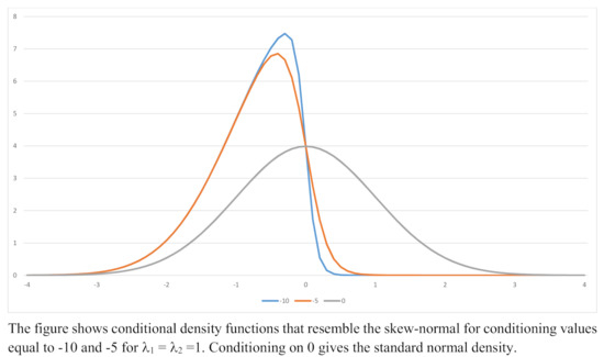
Figure 5. Example Conditional Density Functions; ${\lambda }_{1,2}=1$, $Y_1=-10,-5,0$.

7.2. Marginal and Conditional Distributions—General Results

For the distribution at Equation (54) suppose that $\mathit{X}$ is partitioned into two components of length $n_1$ and $n_2=n-n_1$ and that $\mathit{A}$ and ${\Sigma }$ are partitioned similarly. Thus

$${\mathit{y}}^{\mathit{T}}\mathit{A}\mathit{x}={\mathit{y}}^{\mathit{T}}{\mathit{A}}_1{\mathit{x}}_{\mathbf{1}}+{\mathit{y}}^{\mathit{T}}{\mathit{A}}_2{\mathit{x}}_{\mathbf{2}},$$

(62)

and write ${\tilde{\varphi }}_n\left(\mathit{x};{\Sigma }\right)$ as

$${\tilde{\varphi }}_n\left(\mathit{x};{\Sigma }\right)={\tilde{\varphi }}_{n_1}\left({\mathit{x}}_1;{{\Sigma }}_{11}\right){\tilde{\varphi }}_{n_2}\left({\mathit{x}}_2-\mathit{B}{\mathit{x}}_1;{{\Sigma }}_{2|1}\right),$$

(63)

with $\mathit{B}={{\Sigma }}_{21}{{\Sigma }}_{11}^{-1}$ and ${{\Sigma }}_{2|1}={{\Sigma }}_{22}-{{\Sigma }}_{21}{{\Sigma }}_{11}^{-1}{{\Sigma }}_{12}$. The argument of $\mathrm{\Phi }\left(.\right)$ may be written as

$${\mathit{y}}^{\mathit{T}}\mathit{A}\mathit{x}={\mathit{y}}^{\mathit{T}}\left({\mathit{A}}_1+{\mathit{A}}_2\mathit{B}\right){\mathit{x}}_1+{\mathit{y}}^{\mathit{T}}{\mathit{A}}_2\left({\mathit{x}}_2-\mathit{B}{\mathit{x}}_1\right)$$

(64)

Integration over ${\mathit{x}}_2$ yields the density of the joint distribution of ${\mathit{X}}_1$ and $\mathit{Y}$

$$f\left({\mathit{x}}_1,\mathit{y}\right)=2{\tilde{\varphi }}_{n_1}\left({\mathit{x}}_1;{{\Sigma }}_{11}\right){\tilde{\varphi }}_m\left(\mathit{y};{\Omega }\right)\mathrm{\Phi }\left\{\frac{{\mathit{y}}^{\mathit{T}}\left({\mathit{A}}_1+{\mathit{A}}_2\mathit{B}\right){\mathit{x}}_1}{\sqrt{1+{\mathit{y}}^{\mathit{T}}{\mathit{A}}_2{{\Sigma }}_{2|1}{\mathit{A}}_2^{\mathit{T}}\mathit{y}}}\right\}.$$

(65)

Integration over ${\mathit{X}}_1\left[\mathit{Y}\right]$ recovers the normal distribution of $\mathit{Y}\left[{\mathit{X}}_1\right]$ as expected. The conditional distribution of ${\mathit{X}}_1$ given $\mathit{Y}=\mathit{y}$ is skew-normal with shape parameter

$$\frac{{\left({\mathit{A}}_1+{\mathit{A}}_2\mathit{B}\right)}^T\mathit{y}}{\sqrt{1+{\mathit{y}}^{\mathit{T}}{\mathit{A}}_2{{\Sigma }}_{2|1}{\mathit{A}}_2^{\mathit{T}}\mathit{y}}}.$$

There is no closed form expression for the joint (marginal) density of ${\mathit{X}}_1$ and ${\mathit{Y}}_i;i=1$ or $=2$, except in the very obscure special case for which ${\mathit{A}}_2{{\Sigma }}_{2|1}{\mathit{A}}_2^{\mathit{T}}=\mathbf{0}$.

7.3. Extended Version

Following the approach used in Section 4 and Section 5.4, an extended version of the distribution at Equation (54) has the density function

$$f\left(\mathit{x},\mathit{y}\right)=2{\tilde{\varphi }}_n\left(\mathit{x};{\Sigma }\right){\tilde{\varphi }}_m\left(\mathit{y};\Omega \right)\mathrm{\Phi }\left(\tau \sqrt{1+{\lambda }^2}+\lambda {\mathit{x}}^{\mathit{T}}\mathit{A}\mathit{y}\right)/\Psi \left(\tau ,\lambda \right),$$

(66)

where $\Psi \left(\tau ,\lambda \right)$ is the normalizing constant. Integration with respect to $\mathit{x}$ or $\mathit{y}$ shows that this is given by the n-dimensional integral

$$\Psi \left(\tau ,\lambda \right)={\int }_{-\infty }^{\infty }{\tilde{\varphi }}_n\left(\mathit{x};{\Sigma }\right)\mathrm{\Phi }\left(\frac{\tau \sqrt{1+{\lambda }^2}}{\sqrt{1+{\lambda }^2{\mathit{x}}^{\mathit{T}}\mathit{A}\Omega {\mathit{A}}^{\mathit{T}}\mathit{x}}}\right)\mathit{d}\mathit{x},$$

or alternatively by the m-dimensional integral

$$\Psi \left(\tau ,\lambda \right)={\int }_{-\infty }^{\infty }{\tilde{\varphi }}_m\left(\mathit{y};{\Omega }\right)\mathrm{\Phi }\left(\frac{\tau \sqrt{1+{\lambda }^2}}{\sqrt{1+{\lambda }^2{\mathit{y}}^{\mathit{T}}{\mathit{A}}^{\mathit{T}}{\Sigma }\mathit{A}\mathit{y}}}\right)\mathit{d}\mathit{y}.$$

7.4. Student Version

In the usual way, consider the distribution of $\mathit{X}$ and $\mathit{Y}$ conditional on $S_i=s_i;i=1,2$ where the $S_i$ are independently distributed as ${\chi }_{\left({\nu }_i\right)}^2/{\nu }_i$. The conditional density function is

$$f\left(\mathit{x},\mathit{y}|S_i=s_i;i=1,2\right)=2{\tilde{\varphi }}_n\left(\mathit{x};{\Sigma }/\sqrt{s_1}\right){\tilde{\varphi }}_m\left(\mathit{y};\Omega /\sqrt{s_2}\right)\mathrm{\Phi }\left(\lambda {\mathit{y}}^{\mathit{T}}\mathit{A}\mathit{x}\sqrt{s_1{s}_2}\right)$$

(67)

Standard manipulations give the following expression for the density function of $\mathit{X}$ and $\mathit{Y}$

$$f\left(\mathit{x},\mathit{y}\right)=2{\tilde{\mathit{T}}}_{{\nu }_1,n}\left(\mathit{x},{\Sigma }\right){\tilde{\mathit{T}}}_{{\nu }_2,m}\left(\mathit{y},\Omega \right)E_{S^{*}}\left[\mathrm{\Phi }\left\{\frac{\lambda {\mathit{x}}^{\mathit{T}}\mathit{A}\mathit{y}\sqrt{s_1{s}_2\left({\nu }_1+1\right)\left({\nu }_1+1\right)}}{\sqrt{{\nu }_2+{\mathit{x}}^{\mathit{T}}{{\Sigma }}^{-1}\mathit{x}}\sqrt{{\nu }_2+{\mathit{y}}^{\mathit{T}}{\Omega }^{-1}\mathit{y}}}\right\}\right],$$

(68)

where $E_{S^{*}}$ denotes expectation over the distribution of the variables $S_i;i=1,2$ which are independently distributed as ${\chi }_{({\nu }_i+1)}^2/({\nu }_i+1)$ variables and ${\tilde{\mathit{T}}}_{\nu ,n}\left(\mathit{x},{\Sigma }\right)$ denotes the density function of an n-variate multivariate Student distribution with $\nu$ degrees of freedom , location parameter vector $\mathbf{0}$ and scale matrix ${\Sigma }$. Note that integration over, say, $S_1$ reduces the right hand side of Equation (68) to

$$2{\tilde{\mathit{t}}}_{{\nu }_1,n}\left(\mathit{x},{\Sigma }\right){\tilde{\mathit{t}}}_{{\nu }_2,m}\left(\mathit{y},\Omega \right)E_{S_2}\left\{{\mathit{T}}_{{\nu }_1+1}\left(\mathbb{R}\right)\right\},\mathbb{R}=\frac{\lambda {\mathit{x}}^{\mathit{T}}\mathit{A}\mathit{y}\sqrt{s_2\left({\nu }_1+1\right)\left({\nu }_1+1\right)}}{\sqrt{{\nu }_2+{\mathit{x}}^{\mathit{T}}{{\Sigma }}^{-1}\mathit{x}}\sqrt{{\nu }_2+{\mathit{y}}^{\mathit{T}}{\Omega }^{-1}\mathit{y}}},$$

(69)

which may be computed numerically for given values of $\mathit{x}$ and $\mathit{y}$. An extended version of the distribution may be developed in the same way as in Section 7.3. The expression at (69) becomes

$${\tilde{\mathit{t}}}_{{\nu }_1,n}\left(\mathit{x},{\Sigma }\right){\tilde{\mathit{t}}}_{{\nu }_2,m}\left(\mathit{y},\Omega \right)E_{S_2}\left[{\mathit{T}}_{{\nu }_1+1}\left\{\tau \sqrt{1+{\lambda }^2}+\mathbb{R}\right\}\right]/\Psi \left(\tau ,\lambda \right),$$

(70)

Given the need for numerical computation indicated at Equations (68) and (69), an alternative skew-Student copula may be obtained by extending the distribution described in Section 6.1. The density function is

$$f\left(\mathit{x},\mathit{y}\right)=2{\tilde{\mathit{t}}}_{{\nu }_1,n}\left(\mathit{x},{\Sigma }\right){\tilde{\mathit{t}}}_{{\nu }_2,m}\left(\mathit{y},\Omega \right){\mathit{T}}_{\omega }\left(\lambda {\mathit{x}}^{\mathit{T}}\mathit{A}\mathit{y}\right).$$

An alternative version is

$$f\left(\mathit{x},\mathit{y}\right)=2{\tilde{\mathit{t}}}_{{\nu }_1,n}\left(\mathit{x},{\Sigma }\right){\tilde{\mathit{t}}}_{{\nu }_2,m}\left(\mathit{y},\Omega \right){\mathit{T}}_{\omega }\left(\mathbb{Q}\right);\mathbb{Q}=\frac{\lambda {\mathit{x}}^{\mathit{T}}\mathit{A}\mathit{y}\sqrt{\left({\nu }_1+1\right)\left({\nu }_1+1\right)}}{\sqrt{{\nu }_2+{\mathit{x}}^{\mathit{T}}{{\Sigma }}^{-1}\mathit{x}}\sqrt{{\nu }_2+{\mathit{y}}^{\mathit{T}}{\Omega }^{-1}\mathit{y}}}.$$

Neither of these distributions, however, lead to easily tractable extended versions.

7.5. Stein’s Lemma

This lemma is useful in Portfolio theory and for the computation of moments and cross moments. The treatment in this sub-section follows that in [13].

Let $g(\mathit{X},\mathit{Y})$ be a scalar valued function of $\mathit{X}$ and $\mathit{Y}$ subject to the usual regularity conditions and consider

$$E\left\{\mathit{x}g\left(\mathit{x},\mathit{y}\right)\right\}=2{\int }_{\mathit{y}}{\int }_{\mathit{x}}\mathit{x}g\left(\mathit{x},\mathit{y}\right){\varphi }_n\left(\mathit{x};{\Sigma }\right){\varphi }_m\left(\mathit{y};\Omega \right)\mathrm{\Phi }\left(\lambda {\mathit{x}}^{\mathit{T}}\mathit{A}\mathit{y}\right)d\mathit{x}d\mathit{y}.$$

(71)

The right hand side of Equation (71) is

$$2E_Y\left[\mathrm{\Sigma }{E}_X\left\{{\nabla }_{\mathit{x}}g\left(\mathit{x},\mathit{y}\right)\mathrm{\Phi }\left(\lambda {\mathit{x}}^{\mathit{T}}\mathit{A}\mathit{y}\right)+g\left(\mathit{x},\mathit{y}\right)\lambda \mathit{A}\mathit{y}\varphi \left(\lambda {\mathit{x}}^{\mathit{T}}\mathit{A}\mathit{y}\right)\right\}\right].$$

(72)

This is

$${\Sigma }\left[E\left\{{\nabla }_{\mathit{x}}g\left(\mathit{x},\mathit{y}\right)\right\}+2E_Y\left\{\lambda {\mathit{A}}^{\mathit{T}}\mathit{y}{\int }_{x}g\left(\mathit{x},\mathit{y}\right){\varphi }_n\left(\mathit{x};{\Sigma }\right)\varphi \left({\mathit{x}}^{\mathit{T}}\mathit{A}\mathit{y}\right)dx\right\}\right].$$

(73)

The second term is

$$\sqrt{\frac{2}{\pi }}{E}_{\mathit{y}}\left[\frac{\mathit{A}\mathit{y}}{\sqrt{1+{\mathit{y}}^{\mathit{T}}{\mathit{A}}^{\mathit{T}}{{\Sigma }}^{-1}\mathit{A}\mathit{y}}}{\int }_{\mathit{x}}g\left(\mathit{x},\mathit{y}\right){\varphi }_n\left\{\mathit{x};{\left({{\Sigma }}^{-1}+\mathit{A}{\mathbf{yy}}^{\mathit{T}}{\mathit{A}}^{\mathit{T}}\right)}^{-1}\right\}d\mathit{x}\right]$$

(74)

with a similar expression for $E\left\{\mathit{y}g\left(.\right)\right\}$.

Example 1.

Bivariate case

Let $n=m=1$, ${\Sigma }=\Omega =1$, $\mathit{A}=1$ and $g\left(X,Y\right)=Y$. Then

$$E\left\{Xg\left(X,Y\right)\right\}=E\left(XY\right)=cov\left(X,Y\right).$$

On using the lemma, ${\nabla }_{x}g\left(x\right)=0$ and the second term above is

$$\sqrt{\frac{2}{\pi }}{E}_Y\left[\frac{\lambda y}{\sqrt{1+y^2{\lambda }^2}}{\int }_{-\infty }^{\infty }y{\varphi }_1\left\{x;\left(1+{\lambda }^2{y}^2\right)\right\}dx\right]=\sqrt{\frac{2}{\pi }}{E}_Y\left[\frac{\lambda y^2}{\sqrt{1+y^2{\lambda }^2}}\right],$$

which agrees with Equation (4).

Example 2.

General Case

For the general case, $g\left(\mathit{x},\mathit{y}\right)=y_i$ for $i=1,\cdots ,m$. As above, ${\nabla }_{\mathit{x}}g\left(x\right)=0$ and the second term in the lemma is

$${\Sigma }\sqrt{\frac{2}{\pi }}{E}_Y\left[\frac{{\mathit{A}}^{\mathit{T}}\mathit{y}{y}_i}{\sqrt{1+{\mathit{y}}^{\mathit{T}}{\mathit{A}}^{\mathit{T}}{{\Sigma }}^{-1}\mathit{A}\mathit{y}}}\right].$$

Hence, the cross covariance matrix is

$$E\left({\mathit{XY}}^{\mathit{T}}\right)={\Sigma }{\mathit{A}}^{\mathit{T}}\sqrt{\frac{2}{\pi }}{E}_{\mathit{y}}\left[\frac{{\mathit{yy}}^{\mathit{T}}}{\sqrt{1+{\mathit{y}}^{\mathit{T}}{\mathit{A}}^{\mathit{T}}{{\Sigma }}^{-1}\mathit{A}\mathit{y}}}\right].$$

This expression must be computed numerically and it must equal

$$\sqrt{\frac{2}{\pi }}{E}_{\mathit{x}}\left[\frac{{\mathit{xx}}^{\mathit{T}}}{\sqrt{1+{\mathit{x}}^{\mathit{T}}{\mathit{A}}^{\mathit{T}}{\Omega }^{-1}\mathit{A}\mathit{x}}}\right]\mathit{A}\Omega .$$

Note also that higher order cross moments, that is, $E\left(X_i^p{Y}_j^q\right)$, may also be computed using Stein’s lemma, albeit with numerical integration.

Example 3.

Portfolio Selection

For portfolio selection assume that $\mathit{X}$ denotes asset returns and that $\mathit{Y}$ denotes sources of skewness in the conditional distribution of $\mathit{X}$ given that $\mathit{Y}=\mathit{y}$. This model reflects an empirical feature of some markets, namely that skewness may be time varying. The return on a portfolio with weights $\mathit{w}$ is ${\mathit{w}}^{\mathit{T}}\mathit{X}$. If the utility function is $U\left({\mathit{w}}^{\mathit{T}}\mathit{X}\right)$ the first order conditions for portfolio selection conditional on $\mathit{Y}=\mathit{y}$ contain the term

$$E_{\mathit{x}}\left\{\mathit{X}{U}^{\prime }\left({\mathit{w}}^{\mathit{T}}\mathit{X}\right)\right\}$$

Hence $g\left(\mathit{X}\right)=U^{\prime }\left({\mathit{w}}^{\mathit{T}}\mathit{X}\right)$ and $\nabla g_{\mathit{x}}\left(\mathit{X}\right)=\mathit{w}{U}^{″}\left({\mathit{w}}^{\mathit{T}}\mathit{x}\right)$. Stein’s lemma yields

$${\Sigma }\mathit{w}E\left\{U^{″}\left({\mathit{w}}^{\mathit{T}}\mathit{X}\right)\right\}+2{\Sigma }{E}_{\mathit{y}}\left\{\lambda \mathit{A}\mathit{y}{\int }_{\mathit{x}}{U}^{\prime }\left({\mathit{w}}^{\mathit{T}}\mathit{x}\right){\varphi }_n\left(\mathit{x};{\Sigma }\right)\varphi \left(\lambda {\mathit{x}}^{\mathit{T}}\mathit{A}\mathit{y}\right)d\mathit{x}\right\}.$$

Assuming that the order of integration may be changed the second term is proportional to

$$\left\{\mathit{A}{\int }_{\mathit{y}}\mathit{y}{\varphi }_m\left(\mathit{y};\Omega \right)\varphi \left({\mathit{x}}^{\mathit{T}}\mathit{A}\mathit{y}\right)d\mathit{y}\right\}.$$

which equals zero. Thus, portfolio selection results in a portfolio on the efficient frontier, as expected. Note that if expectations are taken over the conditional distribution of $\mathit{X}$ given $\mathit{Y}=\mathit{y}$ the result is the same as in [24] with appropriate changes of notation.

8. Three Examples

This section of the paper contains three numerical examples, the purpose of which is to illustrate some aspects of the skew-normal copula and related distributions in action. The first presents results for the distribution function of the bivariate skew-normal copula of Section 2, focusing on asymptotic results for tail probability computations. Example two presents specimen estimation results for the bivariate skew-Student copula of Section 6.1. The final illustration has results for the multivariate skew-normal copula that is described in Section 7, specifically the distribution at Equation (53).

8.1. Bivariate Skew-Normal Copula Distribution Function and Related Computations

The distribution function corresponding to the density function at Equation (1) is

$$P\left(X_1\le x_1,X_2\le x_2\right)=2{\int }_{-\infty }^{x_2}{\int }_{-\infty }^{x_1}\varphi \left(s\right)\varphi \left(\mathit{T}\right)\mathrm{\Phi }\left(\lambda s\mathit{T}\right)dsd\mathit{T}.$$

(75)

There is no analytic expression for this integral. For specified values of $x_{1,2}$ it may be computed numerically. For some applications, for example in finance, there is a requirement to compute the distribution function when both $X_{1,2}$ are substantially less than zero. For $\lambda >0$, $x_{1,2}<<0$ and ignoring power of $1/|x_{1,2}|$ greater than 2, the resulting asymptotic expression is

$$2\mathrm{\Phi }\left(x_1\right)\mathrm{\Phi }\left(x_2\right)\mathrm{\Phi }\left(\lambda x_1{x}_2\right)+2\lambda \frac{\varphi \left(x_1\right)\varphi \left(x_2\right)\varphi \left(\lambda x_1{x}_2\right)}{x_1^2{x}_2^2\left(1+x_1^2{\lambda }^2\right)\left(1+x_2^2{\lambda }^2\right)}\left(x_1^2+x_2^2+{\lambda }^2{x}_1^2{x}_2^2\right).$$

(76)

Figure 6 shows an example of the exact and approximate distribution function corresponding to $\lambda =1$. The quantity tabulated is $\sqrt{P\left(X_1\le X^{*},X_2\le X^{*}\right)}$ for values of $X^{*}$ between −5.0 and −0.1. Similar results may be computed for $\lambda <0$. It may be noted that there are combinations of values of $\lambda$, $x_1$ and $x_2$ under which the second term is negligible and $\mathrm{\Phi }\left(\lambda x_1{x}_2\right)\simeq 1$; that is

$$P\left(X_1\le x_1,X_2\le x_2\right)\simeq 2\varphi \left(x_1\right)\varphi \left(x_2\right).$$

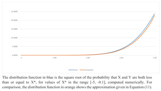
Figure 6. Exact and Approximate Left-hand Quadrant Probabilities; $\lambda =1.0$.

The bivariate skew-normal copula distribution is not specifically suited for financial applications, but it may be used to compute Value at Risk, VaR henceforth. As the variables are standardized, VaR is a critical value in the left hand tail of the distribution $X^{*}$ such that

$$P\left(X_1<x^{*},X_2<x^{*}\right)\simeq 2\mathrm{\Phi }{\left(x^{*}\right)}^2\mathrm{\Phi }\left(\lambda x^{*2}\right)=\alpha ,$$

(77)

for a specified value of $\alpha$ that is small. Conditional Value at Risk, CVaR henceforth, is a related measure. For a single variable X, CVaR is defined as the expected value of X given that it is less than the VaR. For this distribution the properties listed above means that CVaR is the same as that based on the standard normal distribution. A bivariate version of CVaR is defined as

$$E\left(X_1,X_2|X_1\le x^{*},X_2\le x^{*}\right).$$

(78)

For $X_1$ alone this is

$$E\left(X_1|X_1\le x^{*},X_2\le x^{*}\right)={\alpha }^{-1}2{\int }_{-\infty }^{x^{*}}{\int }_{-\infty }^{x^{*}}{x}_1\varphi \left(x_1\right)\varphi \left(x_2\right)\mathrm{\Phi }\left(\lambda x_1{x}_2\right)d{x}_{1}d{x}_2.$$

(79)

For $\lambda >0$ and $x^{*}<<0$, similar arguments to those above lead to

$$E\left(X_1|X_1<x^{*},X_2<x^{*}\right)\simeq -{\alpha }^{-2}\varphi \left(x^{*}\right)\left\{P\left(X_2\le x^{*}|x^{*}\right)+\frac{2\lambda \varphi \left(x^{*}\right)\varphi \left(\lambda x^{*2}\right)}{|x^{*}|{\left(1+x^{*2}{\lambda }^2\right)}^2}\right\},$$

(80)

where $P\left(X_2\le x^{*}|x^{*}\right)$ denotes the distribution function of a standardized skew-normal distribution with shape parameter equal to $\lambda x^{*}$. Using Equation (76) shows that tail dependence equals zero for the skew-normal copula distribution. A Selection of values of CVaR when $\lambda =1$ is shown in Table 9 for critical values ranging from −9.5 to −0.5. The values shown in the second column were computed using numerical inegration. Those in the third column were computed using the asymptotic formula shown at Equation (80). It is suggested that the asymptotic formula leads to values that would be sufficiently accurate for practical purposes.

Table 9. Exact and Asymptotic Values of CVaR; $\lambda =1$.

VaR	Computed	Asymptotic
(CV)	Value	Value
−9.5	−9.5597	−9.6031
−9	−9.0664	−9.1085
−8.5	−8.5722	−8.6146
−8	−8.0787	−8.1214
−7.5	−7.5859	−7.6290
−7	−7.0942	−7.1375
−6.5	−6.6037	−6.6473
−6	−6.1146	−6.1585
−5.5	−5.6273	−5.6714
−5	−5.1423	−5.1865
−4.5	−4.6600	−4.7043
−4	−4.1813	−4.2256
−3.5	−3.7072	−3.7514
−3	−3.2392	−3.2831
−2.5	−2.7793	−2.8227
−2	−2.3307	−2.3732
−1.5	−1.8981	−1.9276
−1	−1.4976	−1.2545
−0.5	−1.1536	−0.2418

8.2. Bivariate Student t Copula

This example is based on the bivariate version of the skew-Student copula of Section 6.1 with ${\mathit{T}}_{\omega }\left(.\right)$ replaced by $\mathrm{\Phi }\left(.\right)$. The density function at Equation (45) becomes

$$f\left(x_1,x_2\right)\hspace{0.17em}=2{\mathit{T}}_{{\nu }_1}\left(x_1\right){\mathit{T}}_{{\nu }_2}\left(x_2\right)\mathrm{\Phi }\left(\lambda x_1{x}_2\right).$$

(81)

First, note that for specified ranges of the shape parameter $\lambda$ this distribution is bimodal. As in Section 2, bimodality requires that $\left|\lambda \right|>\sqrt{\pi /2}$. For the Student case the modal value of X and $\lambda >0$) depends on the degrees of freedom and satisfies

$$\frac{\lambda \sqrt{{\nu }_1{\nu }_2}\left(1+x^2/{\nu }_1\right)}{\sqrt{\left({\nu }_1+1\right)\left({\nu }_2+1\right)\Delta }}{\xi }_1\left(\frac{\lambda \sqrt{{\nu }_2\left({\nu }_1+1\right)}{x}^2}{\sqrt{{\nu }_1\left({\nu }_2+1\right)\Delta }}\right)=1;\Delta =1+\frac{\left({\nu }_2-{\nu }_1\right)x^2}{{\nu }_1\left({\nu }_2+1\right)}.$$

Sets of computed values are shown in Table 10. The first column of the table shows values of $\lambda$. Panel 1 of the table shows the modal value for a set of cases in which the degrees of freedom are equal. Panel 2 shows corresponding values when ${\nu }_1=3$. For comparison purposes, column 2 of panel 2 shows the corresponding modal values for the bivariate skew-normal case.

Table 10. Modal values under the bivariate Student copula.

Panel 1: Equal degrees of freedom
	(3-3)	(5-5)	(7-7)	(10-10)	(20-20)	(50-50)
1.254	0.0000	0.0000	0.0000	0.0000	0.0000	0.0000
3	0.4827	0.5067	0.5169	0.5245	0.5333	0.5387
4	0.4857	0.5013	0.5082	0.5134	0.5195	0.5233
5	0.4714	0.4835	0.4889	0.4929	0.4979	0.5009
15	0.3442	0.3488	0.3509	0.3525	0.3545	0.3557
10	0.3943	0.4007	0.4035	0.4058	0.4085	0.4101
20	0.3101	0.3138	0.3155	0.3168	0.3183	0.3193
35	0.2498	0.2523	0.2534	0.2543	0.2553	0.2559
50	0.2162	0.2181	0.2190	0.2197	0.2205	0.2210
75	0.1826	0.1841	0.1847	0.1853	0.1859	0.1863
100	0.1616	0.1628	0.1633	0.1638	0.1643	0.1646
Panel 2: Unequal degrees of freedom
	SNC	(3-5)	(3-7)	(3-10)	(3-20)	(3-50)
1.254	0.0231	0.0000	0.0000	0.0000	0.0000	0.0000
3	0.5422	0.4894	0.4922	0.4943	0.4966	0.498
4	0.5258	0.4865	0.4868	0.487	0.4871	0.4872
5	0.5029	0.4698	0.4689	0.4683	0.4675	0.4669
15	0.3565	0.3389	0.3365	0.3345	0.3323	0.3308
10	0.4112	0.3894	0.3871	0.3853	0.3832	0.3819
20	0.3200	0.3048	0.3024	0.3005	0.2982	0.2968
35	0.2564	0.2450	0.2428	0.2411	0.2390	0.2377
50	0.2213	0.2118	0.2098	0.2083	0.2064	0.2052
75	0.1865	0.1787	0.1770	0.1757	0.1740	0.1729
100	0.1648	0.1581	0.1565	0.1553	0.1538	0.1529

As in Section 2 the correlation between the two variables is computed numerically. A selection of values is shown in Table 11. The first column of the table shows a range of values of $\lambda$. Panel 1 shows the computed correlation for a selection of cases for which ${\nu }_1={\nu }_2$. The last column shows the corresponding values for the skew-normal copula for comparison. The second panel shows a range of values when ${\nu }_1=3$. The results in the table indicate that the relationship between the shape parameter $\lambda$ and the degrees of freedom is non-linear. Generally, however, correlation is reduced when the degrees of freedom are finite: a noteworthy difference from the bivariate Student distribution.

Table 11. Correlation under the Bivarate Student Copula.

Panel 1: Equal Degrees of Freedom
	(3,3)	(7,7)	(10,10)	(20,20)	(50,50)	Normal
0.01	0.0211	0.0112	0.0100	0.0089	0.0083	0.0080
0.1	0.1369	0.1054	0.0962	0.0867	0.0817	0.0786
1	0.3484	0.4480	0.4527	0.4536	0.4523	0.4505
2	0.3799	0.5185	0.5322	0.5434	0.5482	0.5503
5	0.3972	0.5603	0.5798	0.5980	0.6071	0.6116
10	0.4009	0.5710	0.5919	0.6120	0.6223	0.6268
Panel 2: Unequal Degrees of Freedom
	(3,3)	(3,5)	(3,7)	(3,10)	(3,20)	(3,50)
0.01	0.0211	0.0170	0.0157	0.0148	0.0140	0.0136
0.1	0.1369	0.1301	0.1250	0.1211	0.1167	0.1142
1	0.3484	0.3904	0.3980	0.4015	0.4040	0.4048
2	0.3799	0.4334	0.4452	0.4517	0.4573	0.4600
5	0.3972	0.4579	0.4724	0.4807	0.4885	0.4924
10	0.4009	0.4636	0.4787	0.4876	0.4959	0.5001

To illustrate parameter estimation, the inclusion of scale and location results in the density function

$$f\left(x_1,x_2\right)\hspace{0.17em}=2{\mathit{T}}_{{\nu }_1}\left\{z_1/{\sigma }_1\right\}{\mathit{T}}_{{\nu }_2}\left\{z_2/{\sigma }_2\right\}\mathrm{\Phi }\left(\lambda z_1{z}_2\right)/{\sigma }_1{\sigma }_2;z_i=\hspace{0.17em}\left(x_i-{\mu }_i\right);i=1,2.$$

(82)

Note that this parameterization means that (i) estimators of scale and degrees of freedom are given by the analogous results for a univariate Student’s t distribution, (ii) the estimator of shape depends only on the skewing function $\mathrm{\Phi }$ and its argument and that (iii) only the estimators of location are complicated by the skewing function. Consequently, in the Fisher information [FI] matrix the non-zero off diagonal elements are in the cells corresponding to ${\mu }_{1,2}$ and $\lambda$ and ${\sigma }_i^2$ and ${\nu }_i$; $i=1,2$. Specifically, the FI matrix is

$$\begin{array}{c}\hfill FI=\left[\begin{array}{ccccccc}{l}_{{\mu }_1{\mu }_1}& l_{{\mu }_1{\mu }_2}& 0& 0& l_{{\mu }_1\lambda }& 0& 0\\ l_{{\mu }_2{\mu }_1}& l_{{\mu }_2{\mu }_2}& 0& 0& l_{{\mu }_2\lambda }& 0& 0\\ 0& 0& l_{{\sigma }_1^2{\sigma }_1^2}& 0& 0& l_{{\sigma }_1^2{\nu }_1}& 0\\ 0& 0& 0& l_{{\sigma }_2^2{\sigma }_2^2}& 0& 0& l_{{\sigma }_2^2{\nu }_2}\\ l_{\lambda {\mu }_1}& l_{\lambda {\mu }_2}& 0& 0& l_{\lambda \lambda }& 0& 0\\ 0& 0& l_{{\nu }_1{\sigma }_1^2}& 0& 0& l_{{\nu }_1{\nu }_1}& 0\\ 0& 0& 0& l_{{\nu }_2{\sigma }_2^2}& 0& 0& l_{{\nu }_2{\nu }_2}\end{array}\right],\end{array}$$

where $l_{\theta \theta }$ denotes the expected value of the second derivative of the log-likelihood function with respect to a parameter $\theta$. The non-zero elements of $FI$ to be computed numerically using the distribution at Equation (82) are

$$l_{{\mu }_i{\mu }_i}=-\left({\nu }_i+1\right)/{\sigma }_i^2\left({\nu }_i+3\right)+{\sigma }_j^2{\lambda }^{2}E\left\{z_j^2{\xi }_2\left(\lambda z_i{z}_j\right)\right\};(i,j)=(1,2),(2,1).$$

$$l_{{\mu }_i{\mu }_j}=\lambda E\left\{{\xi }_1\left(\lambda z_i{z}_j\right)\right\}+{\sigma }_i{\sigma }_j{\lambda }^{2}E\left\{z_i{z}_j{\xi }_2\left(\lambda z_i{z}_j\right)\right\},$$

$$l_{{\mu }_i\lambda }=-E\left\{z_j{\xi }_1\left(\lambda z_i{z}_j\right)\right\}+\lambda E\left\{z_i{z}_j^2{\xi }_2\left(\lambda z_i{z}_j\right)\right\},$$

where ${\xi }_1\left(x\right)$ is as defined in Proposition 1 and ${\xi }_2\left(x\right)=-{\xi }_1\left(x\right)\left\{x+{\xi }_1\left(x\right)\right\}$. The remaining elements corresponding to scale and degrees of freedom are the same as those for the FI matrix for Student’s t, namely

$$l_{{\sigma }_i^2{\sigma }_i^2}=-{\nu }_i/2{\sigma }_i^4\left({\nu }_i+3\right);l_{{\sigma }_i^2{\nu }_i}=1/{\sigma }_i^2\left({\nu }_i+1\right)\left({\nu }_i+3\right),$$

and

$$l_{{\nu }_i{\nu }_i}=\left[{\mathrm{\Psi }}^{{}^{\prime }}\left\{\left({\nu }_i+1\right)/2\right\}-{\mathrm{\Psi }}^{{}^{\prime }}\left\{{\nu }_i/2\right\}\right]/4-\left({\nu }_i+5\right)/2{\nu }_i\left({\nu }_i+1\right)\left({\nu }_i+3\right),$$

where ${\mathrm{\Psi }}^{{}^{\prime }}\left(\nu \right)=d^{2}log\Gamma \left(\nu \right)/d{\nu }^2$. These are standard results, but may be found in [25]. The distributions described in this paper all possess the property that the shape parameter may take a value on the boundary of the parameter space. Nonetheless, the FI matrix is inverted and used in the usual way to provide an estimate of the variability of the estimated model parameters. ML estimators of the parameters may be computed using a Newton–Raphson type scheme.

The data set used consists of the weekly returns on 30 stocks that are constituents of the United States S&P500 index. As the example in this subsection and in the following are solely for purposes of illustration, the stocks are numbered. The example in this subsection presents results for 14 pairs of securities, namely stock 1 successively paired with stocks 2 through 15. The computations shown in Table 12 through Table 13 and Table 14 are based on 100 observations.A standard set of descriptive statistics for the 15 stocks is shown in Table 12.

Table 12. Descriptive Statistics, N = 100.

Stock	Mean	St.dev	Min	Max	Skewness	Kurtosis
1	−0.0025	0.0417	−0.1633	0.1125	−0.4161	4.6963
2	−0.0108	0.0968	−0.4700	0.2095	−1.1852	7.9222
3	−0.0010	0.0608	−0.2572	0.2010	−0.5750	8.0273
4	0.0073	0.0428	−0.1168	0.1468	−0.3540	4.3228
5	−0.0008	0.0349	−0.1456	0.0812	−0.9588	5.6347
6	−0.0020	0.0551	−0.2250	0.1707	−0.4596	5.9019
7	−0.0073	0.1030	−0.6183	0.4433	−1.8121	18.8279
8	−0.0003	0.0570	−0.2353	0.1347	−1.1859	7.2066
9	−0.0033	0.0640	−0.4110	0.2298	−1.8642	20.9143
10	0.0004	0.0332	−0.1520	0.1269	−1.2688	9.8876
11	−0.0059	0.0609	−0.1861	0.1891	0.2182	4.6922
12	−0.0066	0.0519	−0.2371	0.1556	−1.1826	9.3188
13	−0.0067	0.0781	−0.2880	0.1402	−0.6467	4.0701
14	−0.0031	0.0659	−0.3898	0.2074	−2.0377	15.2042
15	−0.0018	0.0428	−0.1304	0.127	−0.0926	4.6006

Table 13. Parameter Estimates under the Bivarate Student Copula.

Panel 1: Parameters
	${\mu }_1$	${\mu }_2$	${\sigma }_1^2$	${\sigma }_2^2$	$\lambda$	${\nu }_x$	${\nu }_y$
1-2	−0.0039	−0.0097	0.0011	0.0043	0.0285	4	6
1-3	−0.0018	0.0032	0.0011	0.0009	0.0074	4	4
1-4	−0.0016	0.0111	0.0011	0.0010	0.0161	4	4
1-5	−0.0017	0.0015	0.0011	0.0007	0.0211	4	4
1-6	−0.0006	0.0013	0.0011	0.0014	0.0313	4	6
1-7	−0.0022	−0.0005	0.0011	0.0023	0.0067	4	4
1-8	−0.0011	0.0031	0.0011	0.0017	0.0608	4	4
1-9	−0.0035	−0.0006	0.0011	0.0008	0.0077	4	5
1-10	−0.0010	0.0044	0.0011	0.0004	0.0134	4	4
1-11	−0.0020	−0.0086	0.0011	0.0021	0.0325	4	5
1-12	−0.0057	−0.0053	0.0012	0.0010	0.0205	4	5
1-13	−0.0013	−0.0009	0.0011	0.0036	0.0081	4	4
1-14	−0.0034	0.0027	0.0011	0.0014	0.0189	4	4
1-15	−0.0006	−0.0008	0.0011	0.0011	0.0220	4	5
Panel 2: Estimated standard errors
	${\mu }_1$	${\mu }_2$	${\sigma }_1^2$	${\sigma }_2^2$	$\lambda$	${\nu }_x$	${\nu }_y$
1-2	0.0040	0.0074	0.0003	0.0010	0.0747	1.66	3.45
1-3	0.0040	0.0036	0.0003	0.0002	0.0664	1.66	1.66
1-4	0.0040	0.0037	0.0003	0.0002	0.0664	1.66	1.66
1-5	0.0040	0.0032	0.0003	0.0002	0.0664	1.66	1.66
1-6	0.0040	0.0043	0.0003	0.0003	0.0747	1.66	3.45
1-7	0.0040	0.0057	0.0003	0.0006	0.0664	1.66	1.66
1-8	0.0040	0.0048	0.0003	0.0004	0.0664	1.66	1.66
1-9	0.0040	0.0032	0.0003	0.0002	0.0713	1.66	2.47
1-10	0.0040	0.0024	0.0003	0.0001	0.0664	1.66	1.66
1-11	0.0040	0.0052	0.0003	0.0005	0.0713	1.66	2.47
1-12	0.0040	0.0036	0.0003	0.0002	0.0713	1.66	2.47
1-13	0.0040	0.0071	0.0003	0.0009	0.0664	1.66	1.66
1-14	0.0040	0.0045	0.0003	0.0004	0.0664	1.66	1.66
1-15	0.0040	0.0038	0.0003	0.0003	0.0713	1.66	2.47

Table 14. Critical Values under the bivarate Student copula.

Pair	p = 0.001	p = 0.01	p = 0.05	%err (0.001)	%err (0.01)	%err (0.05)
1-2	−6.3921	−3.5784	−2.1139	8.4613	6.3429	4.9061
1-3	−7.5351	−3.8412	−2.1651	5.0453	2.5150	1.5594
1-4	−7.7466	−3.9225	−2.1976	7.9944	4.6864	3.086
1-5	−7.7792	−3.9714	−2.2139	8.4481	5.9893	3.8494
1-6	−6.4085	−3.5948	−2.1139	8.7405	6.8319	4.9061
1-7	−7.5025	−3.8249	−2.1651	4.5916	2.0807	1.5594
1-8	−7.8117	−4.1341	−2.3115	8.9018	10.3322	8.4292
1-9	−6.7250	−3.6073	−2.0977	4.7312	2.2758	1.5543
1-10	−7.6978	−3.9063	−2.1814	7.3139	4.2521	2.3227
1-11	−6.9876	−3.7714	−2.1633	8.8199	6.9281	4.7320
1-12	−6.9384	−3.7058	−2.1305	8.0533	5.0672	3.1431
1-13	−7.5676	−3.8412	−2.1651	5.499	2.5150	1.5594
1-14	−7.7629	−3.9551	−2.1976	8.2213	5.5550	3.0860
1-15	−6.9384	−3.7222	−2.1469	8.0533	5.5324	3.9376

Table 13 shows estimated parameters for the 14 specified pairs of stocks, computed using the method of maximum likelihood [ML]. Panel 1 shows the estimated parameters. Note that the estimates of the degrees of freedom are shown truncated. Panel 2 shows estimates of parameter precision computed by inverting the FI matrix. The estimated values of the shape parameter $\lambda$ are all positive, consistent with the stylized fact that stock returns are generally positively correlated. There are four other points to note. First, the estimate of the location parameter for stock 1 depends on the choice of the second stock; that is, it is affected by the presence of the skewing factor and the non-zero values of $\lambda$. Secondly, the magnitude of each estimated $\lambda$ in panel 1 is less than the corresponding estimate of parameter precision in panel 2. This suggests that a test of the null hypothesis $H_0:\lambda =0$ would not be rejected against either a one- or two sided alternative. This suggestion, however, is not supported by corresponding likelihood ratio tests reported in Table 15, all of which would lead to rejection of $H_0$. Thirdly, the estimated values of $\lambda$ are all less in magnitude than that required for the distribution to be bi-modal. Finally, it is of interest to inquire if the small estimated values $\lambda$ have much effect on critical values [CVs]. For each of the fourteen pairs of stocks columns 2, 3 and 4 of Table 14 show computed critical values at probabilities of $0.002$, $0.01$ and $0.05$. Columns 5 through 7 show a measure of the effect of the non-zero value of $\lambda$. This is computed as follows. When the degrees of freedom are equal, the CV is computed for Student’s t distribution with the same degrees of freedom. The column entries show the percentage difference. For example, for stock pair 1–3 the Student’s t CV corresponding to a probability of 0.001 is −7.1732. The CV under the model is −7.5351, a difference of abut 5%. When the degrees of freedom for a stock pair are different, the average is taken to compute the Student quantiles. For some applications the differences in the CVs might be regarded as negligible. For other applications they would not.

Table 15. Likelihood ratio tests under the bivarate Student copula.

Pair	${\mathit{logl}}_{\mathit{N}}$	${\mathit{logl}}_{\mathit{STC}}$	$\mathit{lrtest}$	p-Value
1-2	268.3707	413.2626	289.7838	0.0000
1-3	314.8326	467.2746	304.8840	0.0000
1-4	349.8942	484.8219	269.8555	0.0000
1-5	370.2326	509.2042	277.9432	0.0000
1-6	324.6268	469.9988	290.7438	0.0000
1-7	262.1842	425.7775	327.1865	0.0000
1-8	321.3790	474.2957	305.8335	0.000
1-9	309.7183	481.3121	343.1876	0.0000
1-10	375.4270	524.3659	297.8779	0.0000
1-11	314.6729	455.9635	282.5812	0.0000
1-12	330.7399	483.9776	306.4756	0.0000
1-13	289.8306	416.5648	253.4685	0.0000
1-14	306.8000	464.5356	315.4711	0.0000
1-15	350.0291	489.5017	278.9452	0.0000

8.3. Multivariate Skew-Normal Copula

The final illustration uses the multivariate skew-normal copula. The parameterization of the distribution at Equation (53) facilitates estimation. The ML estimators of ${\Sigma }$ and $\Omega$ depend only on the sets of observations $\left\{\mathit{x}\right\}$ and $\left\{\mathit{y}\right\}$, respectively. The ML estimator of $\mathbf{\lambda }$ depends on ${\xi }_1\left(.\right)$. As above, ML parameter estimation requires only a simple Newton–Raphson scheme. The FI matrix has a block structure. The $3n\times 3n$ matrix corresponding to $\mathbf{\mu }$, $\mathbf{\nu }$ and $\mathbf{\lambda }$ is

$$\begin{array}{c}\hfill FI=\left[\begin{array}{ccc}{l}_{\mu {\mu }^{\mathit{T}}}& l_{\mu {\nu }^{\mathit{T}}}& l_{\mu {\lambda }^{\mathit{T}}}\\ l_{\nu {\mu }^{\mathit{T}}}& l_{\nu {\nu }^{\mathit{T}}}& l_{\nu {\lambda }^{\mathit{T}}}\\ l_{\lambda {\mu }^{\mathit{T}}}& l_{\lambda {\nu }^{\mathit{T}}}& l_{\lambda {\lambda }^{\mathit{T}}}\end{array}\right].\end{array}$$

(83)

With the following definitions

$${\mathit{z}}_1=\mathit{x}-\mathit{\mu },{\mathit{z}}_2=\mathit{y}-\mathbf{\nu },{\Lambda }=diag\left({\lambda }_1,\cdots ,{\lambda }_n\right),Q={\mathit{z}}_1{\Lambda }{\mathit{z}}_1,$$

the sub-matrices in the FI matrix are

$$l_{\mu {\mu }^{\mathit{T}}}=-{{\Sigma }}^{-1}+{\Lambda }E\left\{{\mathit{z}}_2{\mathit{z}}_2^{\mathit{T}}{\xi }_2\left(Q\right)\right\},l_{\nu {\nu }^{\mathit{T}}}=-{\Omega }^{-1}+{\Lambda }E\left\{{\mathit{z}}_1{\mathit{z}}_1^{\mathit{T}}{\xi }_2\left(Q\right)\right\},$$

$$l_{\mu {\nu }^{\mathit{T}}}={\Lambda }E\left\{{\xi }_1\left(Q\right)\right\}+{\Lambda }E\left\{{\mathit{z}}_2{\mathit{z}}_1^{\mathit{T}}{\xi }_2\left(Q\right)\right\},l_{\lambda {\lambda }^{\mathit{T}}}=E\left[\left\{\left({\mathit{z}}_1{\mathit{z}}_1^{\mathit{T}}\right)\odot \left({\mathit{z}}_2{\mathit{z}}_2^{\mathit{T}}\right)\right\}{\xi }_2\left(Q\right)\right],$$

$$l_{\lambda {\mu }^{\mathit{T}}}=E\left[\left\{\left(\mathbf{\lambda }{\mathit{z}}_1^{\mathit{T}}\right)\odot \left({\mathit{z}}_2{\mathit{z}}_1^{\mathit{T}}\right)\right\}{\xi }_2\left(Q\right)\right],l_{\lambda {\mu }^{\mathit{T}}}=E\left[\left\{\left(\mathbf{\lambda }{\mathit{z}}_2^{\mathit{T}}\right)\odot \left({\mathit{z}}_1{\mathit{z}}_2^{\mathit{T}}\right)\right\}{\xi }_2\left(Q\right)\right],$$

with all expectations being computed numerically.

For this illustration, a set of 30 US $S\&P500$ stocks are divided into 2 groups each of 15 stocks. Returns are weekly as before and the data set has 500 observations. The standard set of descriptive statistics is shown in Table 16.

Table 16. Multivariate Skew-normal Copula—Descriptive Statistics, N = 500, p = 15.

Stock	Avg (1)	Vol (2)	Min (10)	Max (11)	Skew.s (7)	Kurt.s (8)
1	0.0013	0.0281	−0.1633	0.1125	−0.6504	7.0302
2	−0.0015	0.0645	−0.4700	0.2260	−0.9124	10.2368
3	0.0016	0.0377	−0.2572	0.2010	−0.8089	12.5767
4	0.0047	0.0346	−0.1179	0.1468	−0.3044	4.2946
5	0.0001	0.0252	−0.1456	0.0874	−0.7086	6.5132
6	0.0016	0.0469	−0.3430	0.1707	−0.8131	10.2547
7	0.0019	0.0537	−0.6183	0.4433	−2.9290	52.964
8	0.0009	0.0409	−0.2353	0.1347	−0.6603	7.1881
9	0.0001	0.0383	−0.4110	0.2298	−1.9705	34.2342
10	0.0008	0.0223	−0.152	0.1269	−1.0284	11.6669
11	0.0004	0.0428	−0.1861	0.1891	−0.2347	6.0851
12	−0.0011	0.0319	−0.2371	0.1556	−1.4995	15.5992
13	−0.0018	0.0436	−0.2880	0.1402	−1.0084	9.5305
14	0.0003	0.0492	−0.3898	0.2074	−1.2720	12.9359
15	−0.0003	0.0297	−0.1304	0.1270	−0.3297	6.0096
16	0.0016	0.0367	−0.2390	0.1358	−0.6832	7.7613
17	0.0018	0.0219	−0.1421	0.1063	−0.7507	10.0922
18	0.0019	0.0264	−0.3156	0.1715	−2.9183	47.872
19	0.0018	0.0270	−0.1209	0.1007	−0.3455	5.7724
20	0.0042	0.0301	−0.1118	0.1342	−0.3669	5.6791
21	0.0032	0.0310	−0.2107	0.1495	−0.7606	8.9065
22	0.0017	0.0258	−0.1235	0.0909	−0.3944	5.3920
23	0.0016	0.0216	−0.1517	0.0888	−0.9443	9.9823
24	0.0044	0.0317	−0.3133	0.1586	−1.8778	25.3881
25	0.0014	0.0303	−0.3209	0.1208	−2.6446	30.2787
26	0.0012	0.024	−0.0841	0.0987	0.1249	4.4550
27	0.0018	0.0238	−0.1138	0.1098	−0.2549	6.8268
28	0.0025	0.0318	−0.1724	0.1529	−0.4396	9.2548
29	0.0019	0.0356	−0.2223	0.1114	−0.8660	7.3263
30	0.0004	0.0349	−0.3031	0.1918	−2.1926	22.9448

The ML estimators of location and shape are computed using a Newton–Raphson scheme, with the resulting estimates shown in Table 17. As in the previous section, the FI matrix is inverted to provide estimates of precision. Unlike the bivariate example, several of the shape parameters exhibit estimates that are more than twice the precision in absolute value, the estimate for the stock pair 1 and 16 being an example.

Table 17. Multivariate Skew-normal Copula—Location and Shape Parameter Estimates.

Pair	Locn-X	St.err-X	Locn-Y	St.err-Y	Shape	St.err
1-16	0.0013	0.0013	0.0016	0.0017	0.3870	0.1227
2-17	−0.0015	0.0029	0.0018	0.0010	−0.2022	0.1227
3-18	0.0016	0.0017	0.0020	0.0012	0.2279	0.1295
4-19	0.0047	0.0016	0.0018	0.0012	−0.0076	0.0815
5-20	0.0001	0.0011	0.0042	0.0014	0.1610	0.0811
6-21	0.0016	0.0021	0.0032	0.0014	0.4757	0.1431
7-22	0.0019	0.0024	0.0017	0.0012	0.1762	0.1378
8-23	0.0009	0.0018	0.0016	0.0010	−0.0085	0.0982
9-24	0.0001	0.0018	0.0044	0.0015	0.6524	0.1785
10-25	0.0008	0.0010	0.0015	0.0014	0.3382	0.1333
11-26	0.0004	0.0019	0.0012	0.0011	0.1169	0.0993
12-27	−0.0011	0.0015	0.0018	0.0011	0.1943	0.1192
13-28	−0.0018	0.0020	0.0025	0.0014	0.0699	0.1125
14-29	0.0003	0.0022	0.0019	0.0016	0.5011	0.1303
15-30	−0.0003	0.0014	0.0005	0.0016	0.7160	0.1488

A standard likelihood ratio test has a value of 259.3 and thus leads to rejection of the null hypothesis that all shape parameters equal zero.

9. Concluding Remarks

This paper paper reports the results of an investigation into the properties of a copula-like version of the skew-normal and skew-Student distributions. The distributions studied in the paper allow the marginal distributions to be either normal or Student’s t with differing degrees of freedom. There are several conditional distributions that resemble the skew-normal or are closely related to it. Many of the required computations require numerical integration. The properties of some of the distributions studied depend on certain of the special functions, in particular the G and H functions. There are no explicit expressions available for the moment generating or characteristic functions, although moments and cross moments may be computed when they exist. The examples contained in the paper suggest that parameter estimation is straight forward.

The results show that study of marginal distributions may conceal the nature of a dependence structure and that furthermore there may be different such structures. For future research, there are a number of technical issues concerned with integration. There is also scope for more general results based on unified or generalized skew-elliptical distributions.

Appendix A.1. Proof of Proposition 3

The marginal distribution of X is symmetric and has the density function at Equation (22)

$$f\left(x\right)=\varphi \left(x\right)\mathrm{\Phi }\left({\tilde{\tau }}_x\right)/\Omega \left(\tau ,\lambda \right);{\tilde{\tau }}_x=\tau \sqrt{1+{\lambda }^2}/\sqrt{1+{\lambda }^2{x}^2}.$$

• $E\left(X\right)=0$ by symmetry.
• $var\left(X\right)$ is computed using integration by parts, as follows, omitting the denominator $\Omega \left(.\right)$

  $$var\left(X\right)\propto {\left[-x\varphi \left(x\right)\mathrm{\Phi }\left({\tilde{\tau }}_x\right)\right]}_{-\infty }^{\infty }+{\int }_{-\infty }^{\infty }\varphi \left(x\right)\frac{d}{dx}\left\{x\mathrm{\Phi }\left({\tilde{\tau }}_x\right)\right\}dx.$$
  The first term is zero. The second term is

  $${\int }_{-\infty }^{\infty }\varphi \left(x\right)\mathrm{\Phi }\left({\tilde{\tau }}_x\right)dx-\left\{{\lambda }^2\tau \sqrt{1+{\lambda }^2}\right\}{\int }_{-\infty }^{\infty }\frac{x^2}{{\left(1+{\lambda }^2{x}^2\right)}^{3/2}}\varphi \left({\tilde{\tau }}_x\right)\varphi \left(x\right)dx.$$
  On division by $\Omega \left(\tau ,\lambda \right)$ the first term is equal to unity.
• $cov\left(X,Y\right)$ is also computed using integration by parts. Omitting $\Omega \left(.\right)$ and integrating with respect to y gives

  $$x\varphi \left(x\right)\left\{{\left[-\varphi \left(y\right)\mathrm{\Phi }\left(\tau \sqrt{1+{\lambda }^2}+\lambda xy\right)\right]}_{-\infty }^{\infty }+{\int }_{-\infty }^{\infty }\lambda x\varphi \left(y\right)\varphi \left(\tau \sqrt{1+{\lambda }^2}+\lambda xy\right)dy\right\}.$$
  The term in []s equals zero. On integration with respect to y the second term is

  $$\lambda x\varphi \left({\tilde{\tau }}_x\right)/\sqrt{1+{\lambda }^2{x}^2}.$$
  Integration with respect to x gives the result.
• The conditional distribution at Point 4 follows from dividing Equation (20) by (22).

Appendix A.2. Proof of Proposition 4

• $\Omega \left(\tau ,\lambda \right)$ is given by Equation (21)

  $$\Omega \left(\tau ,\lambda \right)={\int }_{-\infty }^{\infty }\varphi \left(y\right)\mathrm{\Phi }\left(\tau \sqrt{1+{\lambda }^2}/\sqrt{1+{\lambda }^2{y}^2}\right)dy,$$
  Integration by parts and noting tht

  $${\left[\mathrm{\Phi }\left(y\right)\mathrm{\Phi }\left(\tau \sqrt{1+{\lambda }^2}/\sqrt{1+{\lambda }^2{y}^2}\right)\right]}_{-\infty }^{\infty }=1/2,$$

  gives the result.
• Follows directly from Equation (22).
• Follows directly by dividing the joint density function at Equation (20) by Equation (22) and using standard methods.
• The proof employs the asymptotic formula for the standard normal integral in [16] (page 932, Equation 26.2.12); that is

  $$\mathrm{\Phi }\left(x\right)\simeq \varphi \left(x\right)/\left|x\right|;x<<0,$$

  and assumes that higher order terms may be neglected as may integrals of the form

  $${\int }_{-\infty }^x\frac{\varphi \left(s\right)}{s^p}ds\simeq \varphi \left(x\right)/{(-1)}^p{\left|x\right|}^{p+1};x<<0,$$
  In Equation (26) the denominator is.

  $${\mathit{T}}_D={\int }_{-\infty }^y\varphi \left(s\right)\mathrm{\Phi }\left(\tau \sqrt{1+{\lambda }^2}/\sqrt{1+{\lambda }^2{s}^2}\right)ds.$$
  Integrating by parts and using the definition at Equation (23) gives

  $${\mathit{T}}_D=\mathrm{\Phi }\left(y\right)\mathrm{\Phi }\left({\tilde{\tau }}_y\right)-\tau \lambda \sqrt{1+{\lambda }^2}{\int }_{-\infty }^y\frac{\varphi \left(s\right)\mathrm{\Phi }\left({\tilde{\tau }}_s\right)}{{\left(1+{\lambda }^2{s}^2\right)}^{3/2}}ds\simeq \mathrm{\Phi }\left(y\right)\mathrm{\Phi }\left({\tilde{\tau }}_y\right).$$
  The numerator in (26) is

  $${\mathit{T}}_N=\varphi \left(x_1\right){\int }_{-\infty }^y\varphi \left(s\right)\mathrm{\Phi }\left(\tau \sqrt{1+{\lambda }^2}+\lambda x_{1}s\right)ds$$
  Integrating by parts again with ${\tau }^{{}^{\prime }}=\tau \sqrt{1+{\lambda }^2}$ gives

  $${\mathit{T}}_N=\varphi \left(x_1\right)\varphi \left(y\right)\mathrm{\Phi }\left({\tau }^{{}^{\prime }}+\lambda x_{1}y\right)-\lambda x_1\varphi \left(x_1\right){\int }_{-\infty }^y\mathrm{\Phi }\left(s\right)\varphi \left({\tau }^{{}^{\prime }}+\lambda x_{1}s\right)ds.$$
  In the second term in ${\mathit{T}}_N$, $s\le y<<0$, in which case the integrand

  $$\mathrm{\Phi }\left(s\right)\varphi \left({\tau }^{{}^{\prime }}+\lambda x_{1}s\right)\simeq \frac{\varphi \left(s\right)\varphi \left({\tau }^{{}^{\prime }}+\lambda x_{1}s\right)}{\left|s\right|},$$

  may be neglected. Noting that

  $${\tau }^{{}^{\prime }}={\tilde{\tau }}_y\sqrt{1+{\lambda }^2{y}^2},$$

  completes the proof.

References

- Loperfido, N. Skewness-based projection pursuit: A computational approach. Comput. Stat. Data Anal. 2018, 120, 42–57. [Google Scholar] [CrossRef]
- Azzalini, A. A Class of Distributions which Includes The Normal Ones. Scand. J. Stat. 1985, 12, 171–178. [Google Scholar]
- Azzalini, A. Further Results on a Class of Distributions which Includes The Normal Ones. Statistica 1986, 46, 199–208. [Google Scholar]
- Azzalini, A.; Dalla-Valle, A. The Multivariate Skew Normal Distribution. Biometrika 1996, 83, 715–726. [Google Scholar] [CrossRef]
- Azzalini, A.; Capitanio, A. Distributions Generated by Perturbation of Symmetry With Emphasis on a Multivariate Skew t Distribution. J. R. Stat. Soc. Ser. B 2003, 65, 367–389. [Google Scholar] [CrossRef]
- Sahu, S.K.; Dey, D.K.; Branco, M.D. A New Class of Multivariate Skew Distributions with Applications to Bayesian Regression Models. Can. J. Stat. 2003, 31, 129–150. [Google Scholar] [CrossRef]
- Genton, M.G.; Loperfido, N.M. Generalized skew-elliptical distributions and their quadratic forms. Ann. Inst. Stat. Math. 2005, 57, 389–401. [Google Scholar] [CrossRef]
- Arellano-Valle, R.B.; Genton, M.G. Multivariate unified skew-elliptical distributions. Chil. J. Stat. 2010, 926, 17–33. [Google Scholar]
- Bodnar, T.; Mazur, S.; Parolya, N. Central limit theorems for functionals of large sample covariance matrix and mean vector in matrix-variate location mixture of normal distributions. Scand. J. Stat. 2019, 46, 636–660. [Google Scholar] [CrossRef]
- Sklar, A. Fonctions de Répartition à n Dimensions et Leurs Marges. Publ. L’Institut Stat. L’Université Paris 1959, 8, 229–231. [Google Scholar]
- Meijer, C.S. Über Whittakersche bzw. Besselsche Funktionen und deren Produkte. Nieuw Arch. Voor Wiskd. 1936, 18, 10–39. [Google Scholar]
- Fox, C. The G and H Functions as Symmetrical Fourier Kernels. Trans. Am. Math. Soc. 1961, 98, 395–429. [Google Scholar] [CrossRef]
- Adcock, C.J.; Landsman, Z.; Sushi, T. Steins Lemma for generalized skew-elliptical random vectors. Commun. Stat. Theory Methods 2019. [Google Scholar] [CrossRef]
- Stein, C.M. Estimation of The Mean of a Multivariate Normal Distirbution. Ann. Stat. 1981, 9, 1135–1151. [Google Scholar] [CrossRef]
- Gaunt, R.E. Products of Normal, Beta and Gamma Random Variables: Stein Operators and Distributional Theory; Working Paper; The University of Manchester: Manchester, Lancashire, UK, 2016. [Google Scholar]
- Abramowitz, M.; Stegun, I. Handbook of Mathematical Functions; Dover: New York, NY, USA, 1965. [Google Scholar]
- Owen, D.B. Tables for Computing Bivariate Normal Probabilities. Ann. Math. Stat. 1956, 27, 1075–1090. [Google Scholar] [CrossRef]
- Azzalini, A.; Capitanio, A. Statistical Applications of The Multivariate Skew Normal Distribution. J. R. Stat. Soc. Ser. B 1999, 61, 579–602. [Google Scholar] [CrossRef]
- Berg, C.; Vignat, C. On the density of the sum of two independent Student t-random vectors. Stat. Probab. Lett. 2010, 80, 1043–1055. [Google Scholar] [CrossRef]
- Walker, G.A.; Saw, J.G. The Distribution of Linear Combinations of t-Variables. J. Am. Stat. Assoc. 1978, 73, 876–878. [Google Scholar] [CrossRef]
- Loperfido, N. Private Correspondence; Two Items; University of Urbino: Urbino, Italy, 2020. [Google Scholar]
- Adcock, C.J. Private Correspondence; Two Items, March; Sheffield University Management School: Sheffield, UK, 2020. [Google Scholar]
- Loperfido, N. Generalized Skew-Normal Distributions. In Skew-Elliptical Distributions and Their Application: A Journey Beyond Normality; Genton, M., Ed.; CRC/Chapman and Hall: Boca Raton, FL, USA, 2004; pp. 65–80. [Google Scholar]
- Adcock, C.J. Extensions of Stein’s Lemma for the Skew-Normal Distribution. Commun. Stat. Theory Methods 2007, 36, 1661–1671. [Google Scholar] [CrossRef]
- Lange, K.L.; Little, R.J.A.; Taylor, J.M.G. Robust Statistical Modeling Using the t Distribution. J. Am. Stat. Assoc. 1989, 85, 881–896. [Google Scholar] [CrossRef]
Publisher’s Note: MDPI stays neutral with regard to jurisdictional claims in published maps and institutional affiliations. |
© 2021 by the author. Licensee MDPI, Basel, Switzerland. This article is an open access article distributed under the terms and conditions of the Creative Commons Attribution (CC BY) license (https://creativecommons.org/licenses/by/4.0/).