Projected-Reflected Subgradient-Extragradient Method and Its Real-World Applications

Abstract

Our main focus in this work is the classical variational inequality problem with Lipschitz continuous and pseudo-monotone mapping in real Hilbert spaces. An adaptive reflected subgradient-extragradient method is presented along with its weak convergence analysis. The novelty of the proposed method lies in the fact that only one projection onto the feasible set in each iteration is required, and there is no need to know/approximate the Lipschitz constant of the cost function a priori. To illustrate and emphasize the potential applicability of the new scheme, several numerical experiments and comparisons in tomography reconstruction, Nash–Cournot oligopolistic equilibrium, and more are presented.

1. Introduction

In this paper, we focus on the classical variational inequality (VI) problem, as can be found in Fichera [1,2], Stampacchia [3], and Kinderlehrer and Stampacchia [4], defined in real Hilbert space H. Given a nonempty, closed, and convex set of $C\subseteq H$ and a continuous mapping $A:H\to H$, the variational inequality (VI) problem consists of finding a point $x^{*}\in C$ such that:

$$⟨A{x}^{*},x-x^{*}⟩\ge 0\forall x\in C.$$

(1)

$VI(C,A)$ is used to denote the solution set of VIP(1) for simplicity. A wide range of mathematical and applied sciences rely heavily on variational inequalities in both theory and algorithms. Due to the importance of the variational inequality problem and many of its applications in different fields, several notable researchers have extensively studied this class of problems in the literature, and many more new ideas are emerging in connection with the problems. In the case of finite-dimensional setting, the current state-of-the-art results can be found in [5,6,7] including the substantial references therein.

Many algorithms (iterative methods) for solving the variational inequality (1) have been developed and well studied; see [5,6,7,8,9,10,11,12,13,14,15] and the references therein. One of the famous methods is the so-called extragradient method (EGM), which was developed by Korpelevich [16] (also by Antipin [17] independently) in the finite-dimensional Euclidean space for a monotone and Lipschitz continuous operator. The extragradient method has been modified in different ways and later was extended to infinite-dimensional spaces. Many of these extensions were well studied in [18,19,20,21,22,23] and the references therein.

One feature that renders the Korpelevich algorithm less acceptable has to do with the fact that two projections onto the feasible set are required in every iteration. For this reason, there is a need to solve a minimum distance problem twice every iteration. Therefore, the efficiency of this method (Korpelevich algorithm) is affected, which limits its application as well.

A remedy to the second drawback was presented in Censor et al. [18,19,20]. The authors introduced the subgradient-extragradient method (SEGM). Given $x_1\in H$,

$$\begin{array}{c}\hfill \left\{\begin{array}{cc}& y_n=P_C(x_n-\lambda A\left(x_n\right)),\hfill \\ & T_n:=\{w\in H:⟨x_n-\lambda A\left(x_n\right)-y_n,w-y_n⟩\le 0\},\hfill \\ & x_{n+1}=P_{T_n}(x_n-\lambda A\left(y_n\right))\hfill \end{array}\right.\end{array}$$

(2)

In this algorithm, A is an L-Lipschitz-continuous and monotone mapping and ${\displaystyle 0<\lambda <\frac{1}{L}}$. One of the novelties in the proposed SEGM (2) is the replacement of the second projection onto a feasible set with a projection onto a half-space. Recently, weak and strong convergence results of SEGM (2) have been obtained in the literature; see [24,25] and the references therein.

Thong and Hieu in [26] came up with inertial subgradient-extragradient method in the following algorithm. Given $x_0,x_1\in H$,

$$\begin{array}{c}\hfill \left\{\begin{array}{cc}& w_n=x_n+{\theta }_n(x_n-x_{n-1}),\hfill \\ & y_n=P_C(w_n-\lambda A\left(w_n\right)),\hfill \\ & T_n:=\{w\in H:⟨w_n-\lambda A\left(w_n\right)-y_n,w-y_n⟩\le 0\},\hfill \\ & x_{n+1}=P_{T_n}(w_n-\lambda A\left(y_n\right)).\hfill \end{array}\right.\end{array}$$

(3)

The authors proved the weak convergence of the sequence $\left\{x_n\right\}$ generated by (3) to a solution of variational inequality (VI), Equation (1), for the case where A is monotone and an L-Lipschitz-continuous mapping. For some:

$$0<\delta <\frac{1}{2}-2\theta -\frac{1}{2}{\theta }^2,$$

the parameter $\lambda$ is chosen to satisfy:

$$0<\lambda L\le \frac{\frac{1}{2}-2\theta -\frac{1}{2}{\theta }^2-\delta }{\frac{1}{2}-\theta +\frac{1}{2}{\theta }^2}.$$

The sequence $\left\{{\theta }_n\right\}$ is non-decreasing with $0\le {\theta }_n\le \theta <\sqrt{5}-2$.

Malitsky in [21] introduced the following projected reflected gradient method, which solves VI (1) when A is Lipschitz continuous and monotone: choose $x_1,x_0\in C$:

$$\begin{array}{c}\hfill \left\{\begin{array}{cc}& w_n=2x_n-x_{n-1},\hfill \\ & x_{n+1}=P_C(x_n-\lambda A{w}_n),\hfill \end{array}\right.\end{array}$$

(4)

where $\lambda \in (0,\frac{\sqrt{2}-1}{L})$, and we obtain weak convergence results in real Hilbert spaces.

Recently, Bo̧t et al. [27] introduced Tseng’s forward-backward-forward algorithm with relaxation parameters in Algorithm 1 to solve VI (1).

In [28], the following adaptive golden ratio method in Algorithm 2 for solving VI (1) was proposed.

Algorithm 1: Tseng’s forward-backward-forward algorithm with relaxation parameters.

Initialization: Choose ${\rho }_n\in (0,1]$ with the given parameters ${\lambda }_0>0$ and $0<\mu <1$. Let $x_1\in H$ be arbitrary.Iterative steps: $x_{n+1}$ is calculated, with the current iterate $x_n$ given as follows: Step 1. Compute: $$y_n=P_C(x_n-{\lambda }_{n}A{x}_n).$$ If $x_n=y_n$ or $A{y}_n=0$, then stop, and $y_n$ is a solution of $VI(C,A)$. Otherwise: Step 2. Compute: $$x_{n+1}=(1-{\rho }_n)x_n+{\rho }_n(y_n+{\lambda }_n(A{x}_n-A{y}_n)),$$ Update: $${\lambda }_{n+1}=\left\{\begin{array}{cc}min\{{\displaystyle \frac{\mu \parallel x_n-y_n\parallel }{\parallel A{x}_n-A{y}_n\parallel }},{\lambda }_n\}\hfill & ifA{x}_n-A{y}_n\ne 0,\hfill \\ {\lambda }_n\hfill & otherwise.\hfill \end{array}\right.$$ (5) Set $n:=n+1$, and go to Step 1.

Algorithm 2: Adaptive golden ratio method.

Initialization: Choose $x_0,x_1\in H,{\lambda }_0>0,\varphi \in (0,\frac{\sqrt{5}+1}{2}],\overline{\lambda }>0$. Set ${\overline{x}}_0=x_1,{\theta }_0=1,\rho =\frac{1}{\varphi }+\frac{1}{{\varphi }^2}$. Iterative steps: $x_{n+1}$ is calculated, with the current iterate $x_n$ given as follows: Step 1. Compute: $${\lambda }_n=min\left\{\rho {\lambda }_{n-1},\frac{\varphi {\theta }_{n-1}}{4{\lambda }_{n-1}}\frac{\parallel x_n-x_{n-1}{\parallel }^2}{\parallel A{x}_n-A{x}_{n-1}{\parallel }^2},\overline{\lambda }\right\}.$$ Step 2. Compute: $${\overline{x}}_n=\frac{(\varphi -1)x_n+{\overline{x}}_{n-1}}{\varphi },$$ and: $$x_{n+1}=P_C({\overline{x}}_n-{\lambda }_{n}A{x}_n).$$ (6) Update: $${\theta }_n=\frac{{\lambda }_n}{{\lambda }_{n-1}}\varphi$$ (7) Set $n:=n+1$, and go to Step 1.

Motivated by the recent works in [18,19,20,21,26,27,28], our aim in this paper is to introduce a reflected subgradient-extragradient method that solves variational inequalities and obtain weak convergence in the case where the cost function is Lipschitz continuous and a pseudo-monotone operator in real Hilbert spaces. This pseudo-monotone operator is in the sense of Karamardian [29]. Our method uses self-adaptive step sizes, and the convergence of the proposed algorithm is proven without any assumption of prior knowledge of the Lipschitz constant of the cost function.

The outline of the paper is as follows. We start with recalling some basic definitions and results in Section 2. Our algorithm and weak convergence analysis are presented in Section 3. In Section 4, we give some numerical experiments to demonstrate the performances of our method compared with other related algorithms.

2. Preliminaries

In this section, we provide necessary definitions and results needed in the sequel.

Definition 1.

An operator $T:H\to H$ is said to be L-Lipschitz continuouswith $L>0$ if the following inequality is satisfied:

$$\parallel Tx-Ty\parallel \le L\parallel x-y\parallel \forall x,y\in H.$$

Definition 2.

An operator $T:H\to H$ is said to bemonotoneif the following inequality is satisfied:

$$⟨Tx-Ty,x-y⟩\ge 0\forall x,y\in H.$$

Definition 3.

An operator $T:H\to H$ is said to be pseudo-monotone if the following inequality implies the other:

$$⟨Tx,y-x⟩\ge 0⟹⟨Ty,y-x⟩\ge 0\forall x,y\in H.$$

Definition 4.

An operator $T:H\to H$ is said to besequentially weakly continuousif for each sequence $\left\{x_n\right\}$, we have that $x_n$ converges weakly to x, which implies that $\left\{T{x}_n\right\}$ converges weakly to $Tx$.

Recall that for any given point x chosen in H, $P_C\left(x\right)$ denotes the unique nearest point in C. This operator has been shown to be nonexpansive, that is,

$$\parallel x-P_C\left(x\right)\parallel \le \parallel x-y\parallel \forall y\in C.$$

The operator $P_C$ is known as the metric projection of H onto C.

Lemma 1

([30]). Given $x\in H$ and $z\in C$ with C a nonempty, closed, and convex subset of a real Hilbert space H, then:

$$z=P_C\left(x\right)⟺⟨x-z,z-y⟩\ge 0\forall y\in C.$$

Lemma 2

([30,31]). Given $x\in H$, a real Hilbert space and letting C be a closed and convex subset of H, then the following inequalities are true:

1. 

$\parallel P_{C}x-P_C{\left(y\right)\parallel }^2\le ⟨P_{C}x-P_C\left(y\right),x-y⟩\forall y\in H$

2. 

$\parallel P_C{\left(x\right)-y\parallel }^2\le {\parallel x-y\parallel }^2-{\parallel x-P_C\left(x\right)\parallel }^2\forall y\in C.$

Lemma 3

([32]). Given $x\in H$ and $v\in H$, $v\ne 0$, and letting $T=\left\{z\in H:⟨v,z-x⟩\le 0\right\}$, then, for all $u\in H$, the projection $P_T\left(u\right)$ is defined by:

$$P_T\left(u\right)=u-max\left\{0,\frac{⟨v,u-x⟩}{{\left|\right|v\left|\right|}^2}\right\}v.$$

In particular, if $u\notin T$, then:

$$P_T\left(u\right)=u-\frac{⟨v,u-x⟩}{{\left|\right|v\left|\right|}^2}v.$$

The explicit formula provided in Lemma 3 is very important in computing the projection of any point onto a half-space.

Lemma 4

([33], Lemma 2.1). Let $A:C\to H$ be continuous and pseudo-monotone where C is a nonempty, closed, and convex subset of a real Hilbert space H. Then, $x^{*}$ is a solution of $VI(C,A)$ if and only if:

$$⟨Ax,x-x^{*}⟩\ge 0\forall x\in C.$$

Lemma 5

([34]). Let $\left\{x_n\right\}$ be a sequence in H and C a nonempty subset of H with the following conditions satisfied:

(i) 

every sequential weak cluster point of $\left\{x_n\right\}$ is in C;

(ii) 

${\displaystyle \underset{n\to \infty }{lim}\parallel x_n-x\parallel }$ exists for every $x\in C$.

Then, the sequence $\left\{x_n\right\}$ converges weakly to a point in C.

The following lemmas were given in [35].

Lemma 6.

Let h be a real-valued function on a real Hilbert space H, and define $K:=\{x\in H:h(x)\le 0\}$. If h is Lipschitz continuous on H with modulus $\theta >0$ and K is nonempty, then:

$$dist(x,K)\ge \frac{1}{\theta }max\{0,h\left(x\right)\}\forall x\in H,$$

where $dist(x,K)$ is the distance function from x to K.

Lemma 7.

Let H be a real Hilbert space. The following statements are satisfied.

(i) 

For all $x,y\in H$, ${\parallel x+y\parallel }^2={\parallel x\parallel }^2+2⟨x,y⟩+{\parallel y\parallel }^2$;

(ii) 

For all $x,y\in H$, ${\parallel x+y\parallel }^2\le {\parallel x\parallel }^2+2⟨y,x+y⟩$;

(iii) 

For all $x,y\in H$, ${\parallel x+y\parallel }^2={2\parallel x\parallel }^2+{2\parallel y\parallel }^2-{\parallel x-y\parallel }^2$.

Lemma 8

(Maingé [36]). Let $\left\{{\delta }_n\right\}$, $\left\{{\phi }_n\right\}$, and $\left\{{\theta }_n\right\}$ be sequences defined in $[0,+\infty )$ satisfying the following:

$${\phi }_{n+1}\le {\phi }_n+{\theta }_n({\phi }_n-{\phi }_{n-1})+{\delta }_n,\forall n\ge 1,\sum _{n=1}^{+\infty }{\delta }_n<+\infty ,$$

and there exists θ, a real number, with $0\le {\theta }_n\le \theta <1$ for all $n\in \mathbb{N}.$ Then, the following hold:

(i) 

${\displaystyle \sum _{n=1}^{+\infty }{[{\phi }_n-{\phi }_{n-1}]}_{+}<+\infty ,}$ where ${\left[t\right]}_{+}:=max\{t,0\};$

(ii) 

there exists ${\displaystyle {\phi }^{*}\in [0,+\infty )}$ such that ${\displaystyle \underset{n\to \infty }{lim}{\phi }_n={\phi }^{*}.}$

In the work that follows, $x_n\to x$ as $n\to \infty$ denotes the strong convergence of ${\left\{x_n\right\}}_{n=1}^{\infty }$ to a point x, and $x_n\rightharpoonup x$ as $n\to \infty$ denotes the weak convergence of ${\left\{x_n\right\}}_{n=1}^{\infty }$ to a point x.

3. Main Results

We first provide the following conditions upon which the convergence analysis of our method is based and then present our method in Algorithm 3.

Condition 1.

The feasible set C is a nonempty, closed, and convex subset of H.

Condition 2.

The VI (1) associated operator $A:H\to H$ is pseudo-monotone, sequentially weakly and Lipschitz continuous on a real Hilbert space H.

Condition 3.

The solution set of VI (1) is nonempty, that is $VI(C,A)\ne \mathsf{Ø}$.

In addition, we also make the following parameter choices. $0<\alpha \le {\alpha }_n\le {\alpha }_{n+1}<\frac{1}{2+\delta }:=ϵ,\delta >0$.

Remark 1.

We point out here that the proposed Algorithm 3 is different from the method (4) in that the projection step in Algorithm 3 is $P_C(w_n-{\lambda }_{n}A{w}_n)$, while the projection step in (4) is $P_C(x_n-\lambda A{w}_n)$. Furthermore, A is assumed to be pseudo-monotone in our Algorithm 3, while A is assumed to be monotone in (4).

Algorithm 3: Adaptive projected reflected subgradient extragradient method.

Initialization: Given ${\lambda }_0>0,\mu \in (0,1)$, let $x_0,x_1\in H$ be arbitrary Iterative steps: Given the current iterate $x_n$, calculate $x_{n+1}$ as follows: Step 1. Compute: $$\begin{array}{c}\hfill \left\{\begin{array}{cc}& w_n=2x_n-x_{n-1}\hfill \\ & y_n=P_C(w_n-{\lambda }_{n}A{w}_n).\hfill \end{array}\right.\end{array}$$ If $x_n=w_n=y_n=x_{n+1}$, then stop. Otherwise: Step 2. Compute: $$x_{n+1}=(1-{\alpha }_n)x_n+{\alpha }_n{P}_{T_n}\left(w_n\right),$$ where: $$T_n:=\{x\in H:h_n\left(x\right)\le 0\}$$ and $$h_n\left(x\right)=⟨w_n-y_n-{\lambda }_n(A{w}_n-A{y}_n),x-y_n⟩.$$ (8) Update: $${\lambda }_{n+1}=\left\{\begin{array}{cc}min\left\{{\displaystyle \frac{\mu \parallel w_n-y_n\parallel }{\parallel A{w}_n-A{y}_n\parallel }},{\lambda }_n\right\}\hfill & ifA{w}_n-A{y}_n\ne 0,\hfill \\ {\lambda }_n\hfill & otherwise.\hfill \end{array}\right.$$ (9) Set $n:=n+1$, and go to Step 1.

The first step towards the convergence proof of Algorithm 3 is to show that the sequence $\left\{{\lambda }_n\right\}$ generated by (9) is well defined. This is done using similar arguments as in [25].

Lemma 9.

The sequence $\left\{{\lambda }_n\right\}$ generated by (9) is a nonincreasing sequence and:

$$\underset{n\to \infty }{lim}{\lambda }_n=\lambda \ge min\left\{{\lambda }_0,{\displaystyle \frac{\mu }{L}}\right\}.$$

Proof. 

Clearly, by (9), $\left\{{\lambda }_n\right\}$ is nonincreasing since ${\lambda }_{n+1}\le {\lambda }_n$ for all $n\in \mathbb{N}$. Next, using the fact that A is L-Lipschitz continuous, we have:

$$\parallel A{w}_n-A{y}_n\parallel \le L\parallel w_n-y_n\parallel .$$

Therefore, we obtain:

$$\mu {\displaystyle \frac{\parallel w_n-y_n\parallel }{\parallel A{w}_n-A{y}_n\parallel }}\ge {\displaystyle \frac{\mu }{L}}\mathrm{if}A{w}_n\ne A{y}_n,$$

which together with (9) implies that:

$${\lambda }_n\ge min\left\{{\lambda }_0,{\displaystyle \frac{\mu }{L}}\right\}.$$

Therefore, the sequence $\left\{{\lambda }_n\right\}$ is nonincreasing and lower bounded. Therefore, there exists ${lim}_{n\to \infty }{\lambda }_n.$ □

Lemma 10.

Assume that Conditions 1–3 hold. Let $x^{*}$ be a solution of Problem (1) and the function $h_n$ be defined by (8). Then, $h_n\left(x^{*}\right)\le 0$, and there exists $n_0\in \mathbb{N}$ such that:

$$h_n\left(w_n\right)\ge {\displaystyle \frac{1-\mu }{2}}{\parallel w_n-y_n\parallel }^2\forall n\ge n_0.$$

In particular, if $w_n\ne y_n$ then $h_n\left(w_n\right)>0.$

Proof. 

Using Lemma 4 and the fact that $x^{*}$ denotes a solution of Problem (1), we obtain the following:

$$⟨A{y}_n,x^{*}-y_n⟩\le 0.$$

(10)

It follows from (10) and $y_n=P_C(w_n-{\lambda }_{n}A{w}_n)$ that:

$$\begin{array}{cc}\hfill h_n\left(x^{*}\right)& =⟨w_n-y_n-{\lambda }_n(A{w}_n-A{y}_n),x^{*}-y_n⟩\hfill \\ \hfill & =⟨w_n-y_n-{\lambda }_{n}A{w}_n,x^{*}-y_n⟩+{\lambda }_n⟨A{y}_n,x^{*}-y_n⟩\hfill \\ \hfill & \le 0.\hfill \end{array}$$

Hence, the proof of the first claim of Lemma 10 is achieved. Next, we proceed to the proof of the second claim. Clearly, from the definition of $\left\{{\lambda }_n\right\}$, the following inequality is true:

$$\parallel A{w}_n-A{y}_n\parallel \le {\displaystyle \frac{\mu }{{\lambda }_{n+1}}}\parallel w_n-y_n\parallel \forall n.$$

(11)

In fact, Inequality (11) is satisfied if $A{w}_n=A{y}_n$. Otherwise, it implies from (9) that:

$${\lambda }_{n+1}=min\{{\displaystyle \frac{\mu \parallel w_n-y_n\parallel }{\parallel A{w}_n-A{y}_n\parallel }},{\lambda }_n\}\le {\displaystyle \frac{\mu \parallel w_n-y_n\parallel }{\parallel A{w}_n-A{y}_n\parallel }}.$$

Thus,

$$\parallel A{w}_n-A{y}_n\parallel \le {\displaystyle \frac{\mu }{{\lambda }_{n+1}}}\parallel w_n-y_n\parallel .$$

Hence, we can conclude from the above that Inequality (11) is true for $A{w}_n=A{y}_n$ and $A{w}_n\ne A{y}_n$.

Using (11), we obtain:

$$\begin{array}{cc}\hfill h_n\left(w_n\right)& =⟨w_n-y_n-{\lambda }_n(A{w}_n-A{y}_n),w_n-y_n⟩\hfill \\ \hfill & =\parallel w_n-y_n{\parallel }^2-{\lambda }_n⟨A{w}_n-A{y}_n,w_n-y_n⟩\hfill \\ \hfill & \ge \parallel w_n-y_n{\parallel }^2-{\lambda }_n\parallel A{w}_n-A{y}_n\parallel \parallel w_n-y_n\parallel \hfill \\ \hfill & \ge \parallel w_n-y_n{\parallel }^2-\mu {\displaystyle \frac{{\lambda }_n}{{\lambda }_{n+1}}}{\parallel w_n-y_n\parallel }^2\hfill \\ \hfill & =(1-\mu {\displaystyle \frac{{\lambda }_n}{{\lambda }_{n+1}}}){\parallel w_n-y_n\parallel }^2.\hfill \end{array}$$

Since ${lim}_{n\to \infty }(1-\mu {\displaystyle \frac{{\lambda }_n}{{\lambda }_{n+1}}})=1-\mu >{\displaystyle \frac{1-\mu }{2}}>0$, there exists $n_0\in \mathbb{N}$ such that $(1-\mu {\displaystyle \frac{{\lambda }_n}{{\lambda }_{n+1}}})>{\displaystyle \frac{1-\mu }{2}}$ for all $n\ge n_0.$ Therefore,

$$h_n\left(w_n\right)\ge {\displaystyle \frac{1-\mu }{2}}{\parallel w_n-y_n\parallel }^2.$$

□

Remark 2.

Lemma 10 implies that $w_n\notin T_n$ with $n\ge n_0$. Based on Lemma 3, we can write $x_{n+1}$ in the form:

$$x_{n+1}=w_n-{\displaystyle \frac{⟨w_n-y_n-{\lambda }_n(A{w}_n-A{y}_n),w_n-y_n⟩}{\parallel w_n-y_n-{\lambda }_n(A{w}_n-A{y}_n){\parallel }^2}}(w_n-y_n-{\lambda }_n(A{w}_n-A{y}_n))\forall n\ge n_0.$$

We present the following result using similar arguments in [14], Theorem 3.1.

Lemma 11.

Let $\left\{w_n\right\}$ be a sequence generated by Algorithm 3, and assume that Conditions 1–3 hold. Let $\left\{w_n\right\}$ be a sequence generated by Algorithm 3. If there exists $\left\{w_{n_k}\right\}$, a subsequence of $\left\{w_n\right\}$ such that $\left\{w_{n_k}\right\}$ converges weakly to $z\in H$ and ${lim}_{k\to \infty }\parallel w_{n_k}-y_{n_k}\parallel =0$, then $z\in VI(C,A).$

Proof. 

From $w_{n_k}\rightharpoonup z,{lim}_{k\to \infty }\parallel w_{n_k}-y_{n_k}\parallel =0$ and $\left\{y_n\right\}\subset C$, we have $z\in C$.Furthermore, we have:

$$y_{n_k}=P_C(w_{n_k}-{\lambda }_{n_k}A{w}_{n_k}).$$

Thus,

$$⟨w_{n_k}-{\lambda }_{n_k}A{w}_{n_k}-y_{n_k},x-y_{n_k}⟩\le 0\mathrm{for}\mathrm{all}x\in C.$$

Equivalently, we have:

$${\displaystyle \frac{1}{{\lambda }_{n_k}}}⟨w_{n_k}-y_{n_k},x-y_{n_k}⟩\le ⟨A{w}_{n_k},x-y_{n_k}⟩\mathrm{for}\mathrm{all}x\in C.$$

From this, we obtain:

$${\displaystyle \frac{1}{{\lambda }_{n_k}}}⟨w_{n_k}-y_{n_k},x-y_{n_k}⟩+⟨A{w}_{n_k},y_{n_k}-w_{n_k}⟩\le ⟨A{w}_{n_k},x-w_{n_k}⟩\forall x\in C.$$

(12)

We have that $\left\{w_{n_k}\right\}$ is a bounded sequence and A is Lipschitz continuous on H, and we get that $\left\{A{w}_{n_k}\right\}$ is bounded and ${\lambda }_n\ge min\{{\lambda }_0,{\displaystyle \frac{\mu }{L}}\}$. Taking $k\to \infty$ in (12), since $\parallel w_{n_k}-y_{n_k}\parallel \to 0$, we get:

$$\underset{k\to \infty }{lim\; inf}⟨A{w}_{n_k},x-w_{n_k}⟩\ge 0.$$

(13)

On the other hand, we have:

$$⟨A{y}_{n_k},x-y_{n_k}⟩=⟨A{y}_{n_k}-A{w}_{n_k},x-w_{n_k}⟩+⟨A{w}_{n_k},x-w_{n_k}⟩+⟨A{y}_{n_k},w_{n_k}-y_{n_k}⟩.$$

(14)

Since ${lim}_{k\to \infty }\parallel w_{n_k}-y_{n_k}\parallel =0$ and A is Lipschitz continuous on H, we get:

$$\underset{k\to \infty }{lim}\parallel A{w}_{n_k}-A{y}_{n_k}\parallel =0,$$

which, together with (13) and (14), implies that:

$$\underset{k\to \infty }{lim\; inf}⟨A{y}_{n_k},x-y_{n_k}⟩\ge 0.$$

(15)

Next, we show that $z\in VI(C,A)$.

Next, a decreasing sequence, $\left\{{ϵ}_k\right\}$, of positive numbers, which tends to zero, is chosen. We denote by $N_k$, for each k, the smallest positive integer satisfying the inequality:

$$⟨A{y}_{n_j},x-y_{n_j}⟩+{ϵ}_k\ge 0\mathrm{for}\mathrm{all}j\ge N_k.$$

(16)

It should be noted that the existence of $N_k$ is guaranteed by (15). Clearly, the sequence $\left\{N_k\right\}$ is increasing from the fact that $\left\{{ϵ}_k\right\}$ is decreasing. Furthermore, for each k, since $\left\{y_{N_k}\right\}\subset C$, we can suppose $A{y}_{N_k}\ne 0$. We get:

$$⟨A{y}_{N_k},v_{N_k}⟩=1\mathrm{for}\mathrm{each}k,$$

where:

$$v_{N_k}={\displaystyle \frac{A{y}_{N_k}}{\parallel A{y}_{N_k}{\parallel }^2}}.$$

We can infer from (16) that for each k:

$$⟨A{y}_{N_k},x+{ϵ}_k{v}_{N_k}-y_{N_k}⟩\ge 0.$$

Using the pseudo-monotonicity of the operator A on H, we obtain:

$$⟨A(x+{ϵ}_k{v}_{N_k}),x+{ϵ}_k{v}_{N_k}-y_{N_k}⟩\ge 0.$$

Hence, we have:

$$⟨Ax,x-y_{N_k}⟩\ge ⟨Ax-A(x+{ϵ}_k{v}_{N_k}),x+{ϵ}_k{v}_{N_k}-y_{N_k}⟩-{ϵ}_k⟨Ax,v_{N_k}⟩.$$

(17)

Next, we show that:

$$\underset{k\to \infty }{lim}{ϵ}_k{v}_{N_k}=0.$$

Using the fact that $w_{n_k}\rightharpoonup z$ and ${lim}_{k\to \infty }\parallel w_{n_k}-y_{n_k}\parallel =0,$ we get $y_{N_k}\rightharpoonup z\mathrm{as}k\to \infty$. Furthermore, for A sequentially weakly continuous on C, $\left\{A{y}_{n_k}\right\}$ converges weakly to $Az$. We can suppose $Az\ne 0$, since otherwise, z is a solution. Using the fact that the norm mapping is sequentially weakly lower semicontinuous, we obtain:

$$0<\parallel Az\parallel \le \underset{k\to \infty }{lim\; inf}\parallel A{y}_{n_k}\parallel .$$

Since $\left\{y_{N_k}\right\}\subset \left\{y_{n_k}\right\}$ and ${ϵ}_k\to 0$ as $k\to \infty$, we get:

$$\begin{array}{c}\hfill 0\le \underset{k\to \infty }{lim\; sup}\parallel {ϵ}_k{v}_{N_k}\parallel =\underset{k\to \infty }{lim\; sup}\left({\displaystyle \frac{{ϵ}_k}{\parallel A{y}_{n_k}\parallel }}\right)\le {\displaystyle \frac{{lim\; sup}_{k\to \infty }{ϵ}_k}{{lim\; inf}_{k\to \infty }\parallel A{y}_{n_k}\parallel }}=0.\end{array}$$

This in fact means ${lim}_{k\to \infty }{ϵ}_k{v}_{N_k}=0.$

Next, letting $k\to \infty$, then the right-hand side of (17) tends to zero by A being Lipschitz continuous, $\left\{w_{N_k}\right\},\left\{v_{N_k}\right\}$ are bounded, and:

$$\underset{k\to \infty }{lim}{ϵ}_k{v}_{N_k}=0.$$

Hence, we obtain:

$$\underset{k\to \infty }{lim\; inf}⟨Ax,x-y_{N_k}⟩\ge 0.$$

Therefore, for all $x\in C$, we get:

$$⟨Ax,x-z⟩=\underset{k\to \infty }{lim}⟨Ax,x-y_{N_k}⟩=\underset{k\to \infty }{lim\; inf}⟨Ax,x-y_{N_k}⟩\ge 0.$$

Finally, using Lemma 4, we have $z\in VI(C,A)$, which completes the proof. □

Remark 3.

Imposing the sequential weak continuity on A is not necessary when A is a monotone function; see [24].

Theorem 4.

Any sequence $\left\{x_n\right\}$ that is generated using Algorithm 3 converges weakly to an element of $VI(C,A)$ when Conditions 1–3 are satisfied.

Proof. 

Claim 1.$\left\{x_n\right\}$ is a bounded sequence. Define $u_n:=P_{T_n}\left(w_n\right)$, and let $p\in VI(C,A)$. Then, we have:

$$\parallel u_n{-p\parallel }^2=\parallel P_{T_n}{w}_n{-p\parallel }^2\le \parallel w_n{-p\parallel }^2-{\parallel u_n-w_n\parallel }^2.$$

(18)

Furthermore,

$$\begin{array}{cc}\hfill \parallel u_n{-p\parallel }^2={\parallel P_{T_n}{w}_n-p\parallel }^2& \le \parallel w_n{-p\parallel }^2-{\parallel P_{T_n}{w}_n-w_n\parallel }^2\hfill \\ \hfill & =\parallel w_n{-p\parallel }^2-{\mathrm{dist}}^2(w_n,T_n).\hfill \end{array}$$

(19)

This implies that:

$$\begin{array}{ccc}\hfill \parallel x_{n+1}{-p\parallel }^2& =& \parallel (1-{\alpha }_n)(x_n-p)+{\alpha }_n(u_n-p){\parallel }^2\hfill \\ & =& (1-{\alpha }_n)\parallel x_n{-p\parallel }^2+{\alpha }_n{\parallel u_n-p\parallel }^2\hfill \\ & & -{\alpha }_n(1-{\alpha }_n){\parallel x_n-u_n\parallel }^2,\hfill \end{array}$$

(20)

which in turn implies that:

$$\begin{array}{ccc}\hfill \parallel x_{n+1}{-p\parallel }^2& \le & (1-{\alpha }_n)\parallel x_n{-p\parallel }^2+{\alpha }_n{\parallel w_n-p\parallel }^2\hfill \\ & & -{\alpha }_n(1-{\alpha }_n){\parallel x_n-u_n\parallel }^2.\hfill \end{array}$$

(21)

Note that:

$$x_{n+1}=(1-{\alpha }_n)x_n+{\alpha }_n{u}_n$$

and this implies:

$$u_n-x_n=\frac{1}{{\alpha }_n}(x_{n+1}-x_n).$$

(22)

Using (22) in (21), we obtain:

$$\begin{array}{ccc}\hfill \parallel x_{n+1}{-p\parallel }^2& \le & (1-{\alpha }_n){\parallel x_n-p\parallel }^2+{\alpha }_n{\parallel w_n-p\parallel }^2\hfill \\ & & -\frac{(1-{\alpha }_n)}{{\alpha }_n}{\parallel x_{n+1}-x_n\parallel }^2.\hfill \end{array}$$

(23)

Furthermore, by Lemma 7 (iii),

$$\begin{array}{ccc}\hfill \parallel w_n{-p\parallel }^2& =& \parallel 2x_n-x_{n-1}{-p\parallel }^2\hfill \\ & =& \parallel (x_n-p)+(x_n-x_{n-1}){\parallel }^2\hfill \\ & =& 2\parallel x_n{-p\parallel }^2-{\parallel x_{n-1}-p\parallel }^2\hfill \\ & & +2\parallel x_n-x_{n-1}{\parallel }^2.\hfill \end{array}$$

(24)

Using (24) in (23):

$$\begin{array}{ccc}\hfill \parallel x_{n+1}{-p\parallel }^2& \le & (1-{\alpha }_n)\parallel x_n{-p\parallel }^2+2{\alpha }_n{\parallel x_n-p\parallel }^2\hfill \\ & & -{\alpha }_n\parallel x_{n-1}{-p\parallel }^2+2{\alpha }_n{\parallel x_n-x_{n-1}\parallel }^2\hfill \\ & & -\frac{1-{\alpha }_n}{{\alpha }_n}{\parallel x_{n+1}-x_n\parallel }^2\hfill \\ & =& (1+{\alpha }_n)\parallel x_n{-p\parallel }^2-{\alpha }_n{\parallel x_{n-1}-p\parallel }^2\hfill \\ & & +2{\alpha }_n{\parallel x_n-x_{n-1}\parallel }^2\hfill \\ & & -\frac{1-{\alpha }_n}{{\alpha }_n}{\parallel x_{n+1}-x_n\parallel }^2.\hfill \end{array}$$

(25)

Define:

$${\mathsf{\Gamma }}_n:=\parallel x_n{-p\parallel }^2-{\alpha }_n\parallel x_{n-1}{-p\parallel }^2+2{\alpha }_n{\parallel x_n-x_{n-1}\parallel }^2,n\ge 1.$$

Since ${\alpha }_n\le {\alpha }_{n+1}$, we have:

$$\begin{array}{ccc}\hfill {\mathsf{\Gamma }}_{n+1}-{\mathsf{\Gamma }}_n& =& \parallel x_{n+1}{-p\parallel }^2-(1+{\alpha }_{n+1}){\parallel x_n-p\parallel }^2\hfill \\ & & +{\alpha }_n\parallel x_{n-1}{-p\parallel }^2+2{\alpha }_{n+1}{\parallel x_{n+1}-x_n\parallel }^2\hfill \\ & & -2{\alpha }_n{\parallel x_n-x_{n-1}\parallel }^2\hfill \\ & \le & \parallel x_{n+1}{-p\parallel }^2-(1+{\alpha }_n)\parallel x_n{-p\parallel }^2+{\alpha }_n{\parallel x_{n-1}-p\parallel }^2\hfill \\ & & +2{\alpha }_{n+1}{\parallel x_{n+1}-x_n\parallel }^2\hfill \\ & & -2{\alpha }_n{\parallel x_n-x_{n-1}\parallel }^2.\hfill \end{array}$$

(26)

Now, using (25) in (26), one gets:

$$\begin{array}{ccc}\hfill {\mathsf{\Gamma }}_{n+1}-{\mathsf{\Gamma }}_n& \le & -\frac{1-{\alpha }_n}{{\alpha }_n}\parallel x_{n+1}-x_n{\parallel }^2+2{\alpha }_{n+1}{\parallel x_{n+1}-x_n\parallel }^2\hfill \\ & =& -\left(\frac{1-{\alpha }_n}{{\alpha }_n}-2{\alpha }_{n+1}\right){\parallel x_{n+1}-x_n\parallel }^2.\hfill \end{array}$$

(27)

Observe that:

$$\begin{array}{ccc}\hfill \frac{1-{\alpha }_n}{{\alpha }_n}-2{\alpha }_{n+1}& =& \frac{1}{{\alpha }_n}-1-2{\alpha }_{n+1}\hfill \\ & \ge & 2+\delta -1-\frac{2}{2+\delta }\hfill \\ & =& \delta +\frac{\delta }{2+\delta }\ge \delta .\hfill \end{array}$$

(28)

Using (28) in (27), we get:

$${\mathsf{\Gamma }}_{n+1}-{\mathsf{\Gamma }}_n\le -\delta {\parallel x_{n+1}-x_n\parallel }^2.$$

(29)

Hence, $\left\{{\mathsf{\Gamma }}_n\right\}$ is non-increasing. In a similar way, we obtain:

$$\begin{array}{ccc}\hfill {\mathsf{\Gamma }}_n& =& \parallel x_n{-p\parallel }^2-{\alpha }_n\parallel x_{n-1}{-p\parallel }^2+2{\alpha }_n{\parallel x_n-x_{n-1}\parallel }^2\hfill \\ & \ge & \parallel x_n{-p\parallel }^2-{\alpha }_n{\parallel x_{n-1}-p\parallel }^2.\hfill \end{array}$$

(30)

Note that:

$${\alpha }_n<\frac{1}{2+\delta }=ϵ<1.$$

From (30), we have:

$$\begin{array}{ccc}\hfill \parallel x_n{-p\parallel }^2& \le & {\alpha }_n{\parallel x_{n-1}-p\parallel }^2+{\mathsf{\Gamma }}_n\hfill \\ & \le & ϵ\parallel x_{n-1}{-p\parallel }^2+{\mathsf{\Gamma }}_1\hfill \\ & ⋮\\ & \le & {ϵ}^n{\parallel x_0-p\parallel }^2+(1+\cdots +{ϵ}^{n-1}){\mathsf{\Gamma }}_1\hfill \\ & \le & {ϵ}^n{\parallel x_0-p\parallel }^2+\frac{{\mathsf{\Gamma }}_1}{1-ϵ}.\hfill \end{array}$$

(31)

Consequently,

$$\begin{array}{ccc}\hfill {\mathsf{\Gamma }}_{n+1}& =& \parallel x_{n+1}{-p\parallel }^2-{\alpha }_{n+1}{\parallel x_n-p\parallel }^2\hfill \\ & & +2{\alpha }_{n+1}{\parallel x_{n+1}-x_n\parallel }^2\hfill \\ & \ge & -{\alpha }_{n+1}{\parallel x_n-p\parallel }^2\hfill \end{array}$$

and this means from (31) that:

$$\begin{array}{ccc}\hfill -{\mathsf{\Gamma }}_{n+1}& \le & {\alpha }_{n+1}{\parallel x_n-p\parallel }^2\hfill \\ & \le & ϵ\parallel x_n{-p\parallel }^2\hfill \\ & ⋮\\ & \le & {ϵ}^{n+1}{\parallel x_0-p\parallel }^2+\frac{ϵ{\mathsf{\Gamma }}_1}{1-ϵ}.\hfill \end{array}$$

(32)

By (29) and (32), we get:

$$\begin{array}{ccc}\hfill \delta \sum _{n=1}^k{\parallel x_{n+1}-x_n\parallel }^2& \le & {\mathsf{\Gamma }}_1-{\mathsf{\Gamma }}_{k+1}\hfill \\ & \le & {ϵ}^{k+1}{\parallel x_0-p\parallel }^2+\frac{{\mathsf{\Gamma }}_1}{1-ϵ}.\hfill \end{array}$$

(33)

This then implies that:

$$\sum _{n=1}^{\infty }{\parallel x_{n+1}-x_n\parallel }^2\le \frac{{\mathsf{\Gamma }}_1}{\delta (1-ϵ)}<+\infty .$$

(34)

Hence, $\underset{n\to \infty }{lim}\parallel x_{n+1}-x_n\parallel =0.$ We also have from Algorithm 3 that:

$$\begin{array}{c}\hfill \parallel w_n-x_n\parallel =\parallel x_n-x_{n-1}\parallel \to 0,n\to \infty .\end{array}$$

(35)

From (25), we obtain:

$$\begin{array}{ccc}\hfill \parallel x_{n+1}{-p\parallel }^2& \le & (1+{\alpha }_n)\parallel x_n{-p\parallel }^2-{\alpha }_n{\parallel x_{n-1}-p\parallel }^2\hfill \\ & & +2{\parallel x_n-x_{n-1}\parallel }^2.\hfill \end{array}$$

(36)

Using Lemma 8 in (36) (noting (34)), we get:

$$\begin{array}{c}\hfill \underset{n\to \infty }{lim}{\parallel x_n-p\parallel }^2=l<\infty .\end{array}$$

(37)

This implies that ${lim}_{n\to \infty }\parallel x_n-p\parallel$ exists. Therefore, the sequence $\left\{x_n\right\}$ is bounded, and so is $\left\{y_n\right\}$.

Claim 2. There exists $M>1$ such that:

$${\left[{\displaystyle \frac{1}{M}}{\displaystyle \frac{1-\mu }{2}}{\parallel w_n-y_n\parallel }^2\right]}^2\le \parallel w_n{-p\parallel }^2-{\parallel u_n-p\parallel }^2\forall n\ge n_0.$$

We know that $\left\{A{w}_n\right\},\left\{A{y}_n\right\}$ are bounded using the fact that $\left\{x_n\right\},\left\{y_n\right\},\left\{w_n\right\}$ are bounded. Hence, there exists $M>1$ such that:

$$\parallel w_n-y_n-{\lambda }_n(A{w}_n-A{y}_n)\parallel \le M\mathrm{for}\mathrm{all}n.$$

Therefore, for all $u,v\in H$, we obtain:

$$\begin{array}{cc}\hfill \parallel h_n\left(u\right)-h_n\left(v\right)\parallel & =\parallel ⟨w_n-y_n-{\lambda }_n(A{w}_n-A{y}_n),u-v⟩\parallel \hfill \\ \hfill & \le \parallel w_n-y_n-{\lambda }_n(A{w}_n-A{y}_n)\parallel \parallel u-v\parallel \hfill \\ \hfill & \le M\parallel u-v\parallel .\hfill \end{array}$$

Then, we have that $h_n(·)$ is M-Lipschitz continuous on H. From Lemma 6, we get:

$$\mathrm{dist}(w_n,T_n)\ge {\displaystyle \frac{1}{M}}{h}_n\left(w_n\right),$$

from which, together with Lemma 10, we get:

$$\mathrm{dist}(w_n,T_n)\ge {\displaystyle \frac{1}{M}}{\displaystyle \frac{1-\mu }{2}}{\parallel w_n-y_n\parallel }^2\forall n\ge n_0.$$

(38)

Combining (19) and (38), we obtain:

$${\parallel u_n-p\parallel }^2\le {\parallel w_n-p\parallel }^2-{\left[{\displaystyle \frac{1}{M}}{\displaystyle \frac{1-\mu }{2}}{\parallel w_n-y_n\parallel }^2\right]}^2\forall n\ge n_0.$$

(39)

This complete the proof of Claim 2.

Claim 3. The sequence $\left\{x_n\right\}$ converges weakly to an element of $VI(C,A).$ Indeed, since $\left\{x_n\right\}$ is a bounded sequence, there exists the subsequence $\left\{x_{n_k}\right\}$ of $\left\{x_n\right\}$ such that $x_{n_k}\rightharpoonup z\in C$. Since $\left\{w_n\right\}$ and $\left\{u_n\right\}$ are bounded, there exists $M^{*}>0$ such that $\forall n\ge n_0$, and we have from (39):

$$\begin{array}{ccc}\hfill {\left[{\displaystyle \frac{1}{M}}{\displaystyle \frac{1-\mu }{2}}{\parallel w_n-y_n\parallel }^2\right]}^2& \le & {\parallel w_n-p\parallel }^2-{\parallel u_n-p\parallel }^2\hfill \\ & =& \left[\parallel w_n-p\parallel -\parallel u_n-p\parallel \right]\left[\parallel w_n-p\parallel +\parallel u_n-p\parallel \right]\hfill \\ & \le & \parallel w_n-u_n\parallel \left[\parallel w_n-p\parallel +\parallel u_n-p\parallel \right]\hfill \\ & \le & M^{*}\parallel w_n-u_n\parallel .\hfill \end{array}$$

(40)

From (40), we have:

$$\underset{n\to \infty }{lim}\parallel w_n-y_n\parallel =0.$$

(41)

Consequently,

$$\parallel x_n-y_n\parallel \le \parallel w_n-y_n\parallel +\parallel w_n-x_n\parallel \to 0,n\to \infty .$$

Furthermore, $\left\{w_{n_k}\right\}$ of $\left\{w_n\right\}$ converges weakly to $z\in C$. This implies from Lemma 11 and (41) that $z\in VI(C,A)$. Therefore, we proved that if $p\in VI(C,A)$, then ${lim}_{n\to \infty }\parallel x_n-p\parallel$ exists, and each sequential weak cluster point of the sequence $\left\{x_n\right\}$ is in $VI(C,A)$. By Lemma 5, the sequence $\left\{x_n\right\}$ converges weakly to an element of $VI(C,A).$ □

4. Numerical Illustrations

In this section, we consider many examples in which some are real-life applications for numerical implementations of our proposed Algorithm 3. For a broader overview of the efficiency and accuracy of our proposed algorithm, we investigate and compare the performance of the proposed Algorithm 3 with Algorithm 1 proposed by Boţ et al. in [27] (Bot Alg.), Algorithm 2 proposed by Malitsky in [28] (Malitsky Alg.), the algorithm proposed by Shehu and Iyiola in [37] (Shehu Alg.), the subgradient-extragradient method (SEM) (2), and the extragradient method (EGM) in [16].

Example 1

(Tomography reconstruction model). In this example, we consider the linear inverse problem:

$$Bx=\widehat{b},$$

(42)

where $x\in {\mathbb{R}}^k$ is the unknown image, $B\in {\mathbb{R}}^{m\times k}$ is the projection matrix, and $\widehat{b}\in {\mathbb{R}}^m$ is the given sinogram (set of projections). The aim then is to recover a slice image of an object from a sinogram. To be realistic, we consider noisy $b=\widehat{b}+ϵ$, where $ϵ\in {\mathbb{R}}^m$. Problem (42) can be presented as a convex feasibility problem (CFP) with the sets (hyper-planes) $C_i=\{x:⟨a_i,x⟩=b_i\}$. Since, in practice, the projection matrix B is often rank-deficient, so $b\notin$ range(B); thus, we may assume that the CFP has no solution (also called inconsistent), so we consider the least squares model ${min}_x{\sum }_{i=1}^m\mathrm{dist}{(x,C_i)}^2$.

Recall that the projection onto the hyper-plane $C_i$ has a closed formula $P_{C_i}x=x-\frac{⟨a_i,x⟩-b_i}{\parallel a_i{\parallel }^2}{a}_i$. Therefore, the evaluation of $Tx$ reduces to a matrix-vector multiplication, and this can be realized very efficiently, where $T:=\frac{1}{m}(P_{C_1}+\dots +P_{C_m})$ and $A:=I-T$. Note that our approach only exploits feasibility constraints, which is definitely not a state-of-the-art model for tomography reconstruction. More involved methods would solve this problem with the use of some regularization techniques, but we keep such a simple model for illustration purposes only.

As a particular problem, we wish to reconstruct the Shepp–Logan phantom image $128\times 128$ (thus, $x\in {\mathbb{R}}^k$ with $k=2^8$) from the far less measurement $m=2^7$. We generate the matrix $B\in {\mathbb{R}}^{m\times k}$ randomly and define $b=Bx+ϵ$, where $ϵ\in {\mathbb{R}}^m$ is a random vector, whose entries are drawn from $N(0,1)$.

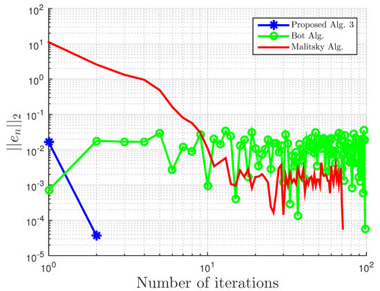
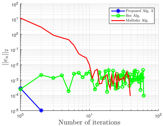
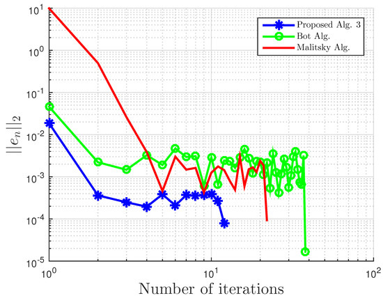
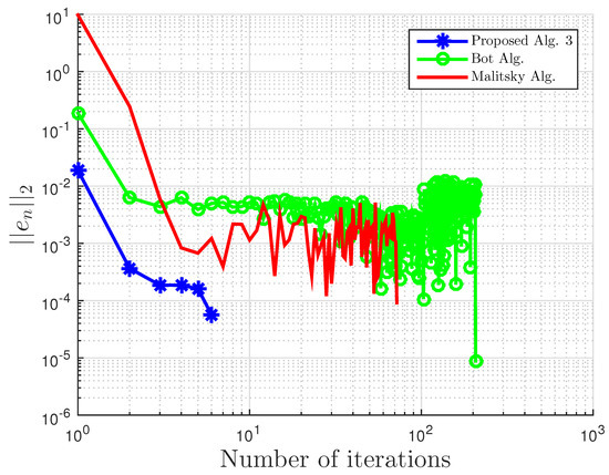
Using this example, we give some comparisons of our proposed Algorithm 3, Algorithm 1 proposed by Boţ et al. in [27] (Bot Alg.), and Algorithm 2 proposed by Malitsky et al. in [28] (Malitsky Alg.) using the residual ${\parallel e_n\parallel }_2:={\parallel x_{n+1}-x_n\parallel }_2\le ϵ$, where $ϵ={10}^{-4}$, as our stopping criterion. For our proposed algorithm, the starting point $x_0$ is chosen randomly with $x_1=(0,\dots ,0)$ and ${\alpha }_n=0.002,$ for Boţ et al., the starting point $x_0=(0,\dots ,0)$ and ${\rho }_n=0.2$, while for Malitsky et al., the starting point $x_0={\overline{x}}_0=(0,\dots ,0)$ with $x_1$ randomly chosen, ${\theta }_0=1,$ and $\overline{\lambda }=1$. All results are reported in Table 1 and Table 2 and Figure 1, Figure 2, Figure 3, Figure 4, Figure 5 and Figure 6.

Table 1. Example 1 comparison: proposed Algorithm 3, Bot Algorithm 1, and Malitsky Algorithm 2 with $\mu =\varphi =0.9$.

	Proposed Algorithm 3		Bot Algorithm 1		Malitsky Algorithm 2
${\mathit{\lambda }}_0$	No. of Iter.	CPU Time	No. of Iter.	CPU Time	No. of Iter.	CPU Time
0.1	2	$5.8318\times {10}^{-3}$	98	0.2590	71	0.1533
1	2	$4.3773\times {10}^{-3}$	61	0.1643	39	0.0826
5	12	$4.0209\times {10}^{-2}$	38	0.1012	22	0.0491
10	6	$1.8319\times {10}^{-2}$	207	0.5764	72	0.1359

Table 2. Example 1: proposed Algorithm 3 with ${\lambda }_0=1$ for different $\mu$ values.

	${\mathit{\lambda }}_0=0.1$	${\mathit{\lambda }}_0=0.3$	${\mathit{\lambda }}_0=0.7$	${\mathit{\lambda }}_0=0.9$
No. of Iter.	6	6	3	2
CPU Time	$2.6506\times {10}^{-2}$	$2.7113\times {10}^{-2}$	$7.1002\times {10}^{-3}$	$4.7982\times {10}^{-3}$

Figure 1. Example 1: $\mu =\varphi =0.9$ and ${\lambda }_0=0.1$. Alg., Algorithm.

Figure 2. Example 1: $\mu =\varphi =0.9$ and ${\lambda }_0=1$.

Figure 3. Example 1: $\mu =\varphi =0.9$ and ${\lambda }_0=5$.

Figure 4. Example 1: $\mu =\varphi =0.9$ and ${\lambda }_0=10$.

Figure 5. Example 1: $\mu =\varphi =0.9$.

Figure 6. Example 1: ${\lambda }_0=1$.

Example 2

(Equilibrium-optimization model). Here, we consider the Nash–Cournot oligopolistic equilibrium model in electricity markets. Given m companies, such that the i-th company possesses $I_i$ generating units, denote by x the power vector, that is each of its j-th entries $x_j$ corresponds to the power generated by unit j. Assume that the price function $p_i$ is an affine decreasing function of $s:={\sum }_{j=1}^N{x}_j$ where N is the number of all generating units. Therefore, $p_i\left(s\right):=\alpha -{\beta }_{i}s$. We can now present the profit of company i as $f_i\left(x\right):=p_i\left(s\right){\sum }_{j\in I_i}{x}_j-{\sum }_{j\in I_i}{c}_j\left(x_j\right)$, where $c_j\left(x_j\right)$ is the cost for generating $x_j$ by generating unit j. Denote by $K_i$ the strategy set of the i-th company i. Clearly, ${\sum }_{j\in I_i}{x}_j\in K_i$ for each i, and the overall strategy set is $C:=K_1\times K_2\times \dots \times K_m$.

The Nash equilibrium concept with regards to the above data is that each company wishes to maximize its profit by choosing the corresponding production level under the presumption that the production of the other companies is a parametric input.

Recall that $x^{*}\in C=K_1\times K_2\times \dots \times K_m$ is an equilibrium point if:

$$f_i\left(x^{*}\right)\ge f_i\left(x^{*}\left[x_i\right]\right)\forall x_i\in K_i,i=1,2,\dots ,m,$$

where the vector $x^{*}\left[x_i\right]$ stands for the vector obtained from $x^{*}$ by replacing $x_i^{*}$ with $x_i$. Define:

$$f(x,y):=\psi (x,y)-\psi (x,x)$$

with:

$$\psi (x,y):=-\sum _{i=1}^n{f}_i\left(x^{*}\left[y_i\right]\right).$$

Therefore, finding a Nash equilibrium point is formulated as:

$$\begin{array}{c}\hfill X^{*}\in C:f(x^{*},x)\ge 0\forall x\in C.\end{array}$$

(43)

Suppose for every j, the cost $c_j$ for production and the environmental fee g are increasingly convex functions. This convexity assumption implies that (43) is equivalent to (see [38]):

$$\begin{array}{c}\hfill x\in C:⟨Bx-a+\nabla \phi \left(x\right),y-x⟩\ge 0\forall y\in C,\end{array}$$

where:

$$\begin{array}{c}a:={(\alpha ,\alpha ,\dots ,\alpha )}^T\hfill \\ B_1=\left(\begin{array}{ccccc}{\beta }_1& 0& 0& \dots & 0\\ 0& {\beta }_2& 0& \dots & 0\\ \dots & \dots & \dots & \dots & \dots \\ 0& 0& 0& 0& {\beta }_m\end{array}\right)B=\left(\begin{array}{ccccc}0& {\beta }_1& {\beta }_1& \dots & {\beta }_1\\ {\beta }_2& 0& {\beta }_2& \dots & {\beta }_2\\ \dots & \dots & \dots & \dots & \dots \\ {\beta }_m& {\beta }_m& {\beta }_m& \dots & {\beta }_m\end{array}\right)\hfill \\ \phi \left(x\right):=x^T{B}_{1}x+\sum _{j=1}^N{c}_j\left(x_j\right).\hfill \end{array}$$

Note that $c_j$ is differentiable convex for every j.

Our proposed scheme is tested with the following cost function:

$$c_j\left(x_j\right)=\frac{1}{2}{x}_j^{T}D{x}_j+d^T{x}_j.$$

The parameters ${\beta }_j$ for all $j=1,\dots ,m$, matrix D, and vector d were generated randomly in the interval $(0,1]$, $[1,40]$, and $[1,40]$, respectively.

The numerical experiments involve the initial points $x_0$ and $x_1$ generated randomly in $[1,40]$ and $m=10$. The stopping role of the algorithm is chosen as ${\parallel e_n\parallel }_2:={\parallel x_{n+1}-x_n\parallel }_2\le ϵ$, where $ϵ={10}^{-4}$. Let us assume that each company has the same lower production bound one and upper production bound 40, that is,

$$K_i:=\{x_i:1\le x_i\le 40\},i=1,\dots ,10.$$

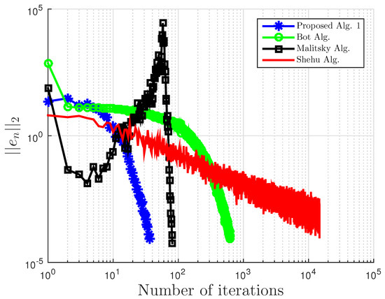
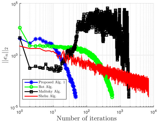
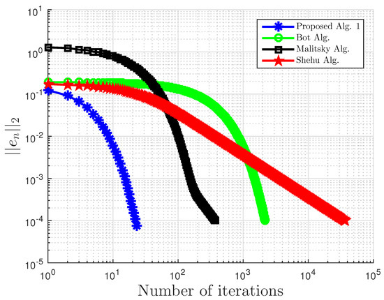
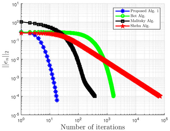
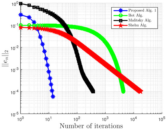
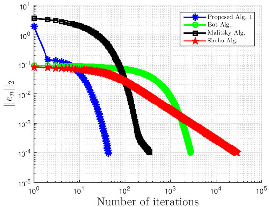
We compare our proposed Algorithm 3 with Algorithm 1 proposed by Boţ et al. in [27] (Bot Alg.), Algorithm 2 proposed by Malitsky et al. in [28] (Malitsky Alg.), and Shehu and Iyiola’s proposed Algorithm 3.2 in [37] (Shehu Alg.). For our proposed algorithm, we choose ${\alpha }_n=0.49,$ for Boţ et al., ${\rho }_n=0.02,$ for Malitsky et al., the starting point $x_0={\overline{x}}_0,$ ${\theta }_0=1,$ and $\overline{\lambda }=1$, while for Shehu and Iyiola, $\rho =1$ and $\sigma =0.5.$ All results are reported in Table 3 and Table 4 and Figure 7, Figure 8, Figure 9, Figure 10, Figure 11 and Figure 12.

Table 3. Example 2 comparison: proposed Algorithm 3, Bot Algorithm 1, Malitsky Algorithm 2, and Shehu Alg. [37] with ${\lambda }_0=1$ and $\mu =\varphi =\gamma$.

	Proposed Algorithm 3		Bot Algorithm 1		Malitsky Algorithm 2		Shehu Alg. [37]
$\mathit{\mu }$	No. of Iter.	CPU Time	No. of Iter.	CPU Time	No. of Iter.	CPU Time	No. of Iter.	CPU Time
0.1	22	$8.7749\times {10}^{-3}$	582	0.1372	33	$8.4833\times {10}^{-3}$	15680	8.7073
0.3	24	$8.8605\times {10}^{-3}$	594	0.1440	47	$9.3949\times {10}^{-3}$	13047	7.2304
0.7	36	$1.8575\times {10}^{-2}$	619	0.1914	81	$1.9522\times {10}^{-2}$	14736	9.8807
0.999	47	$3.9262\times {10}^{-2}$	581	0.3016	1809	0.7438	7048	5.4446

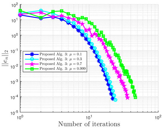
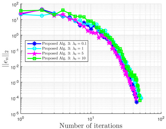
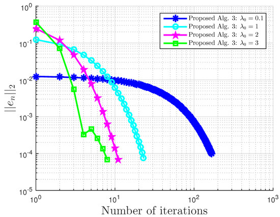
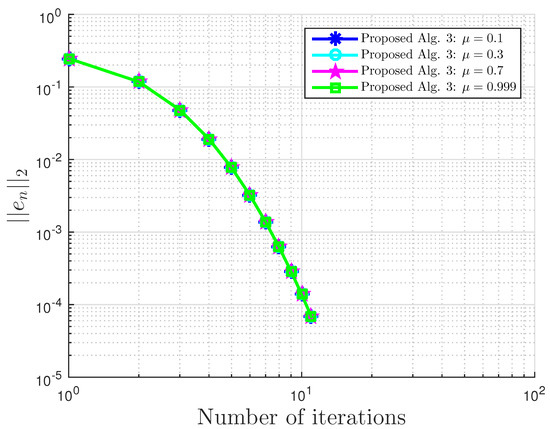
Table 4. Example 2: proposed Algorithm 3 with $\mu =0.999$ for different ${\lambda }_0$ values.

	${\mathit{\lambda }}_0=0.1$	${\mathit{\lambda }}_0=1$	${\mathit{\lambda }}_0=5$	${\mathit{\lambda }}_0=10$
No. of Iter.	45	52	44	50
CPU Time	$2.6624\times {10}^{-2}$	$2.1446\times {10}^{-2}$	$1.7123\times {10}^{-2}$	$1.9696\times {10}^{-2}$

Figure 7. Example 2: $\mu =\varphi =\gamma =0.1$ and ${\lambda }_0=1$.

Figure 8. Example 2: $\mu =\varphi =\gamma =0.3$ and ${\lambda }_0=1$.

Figure 9. Example 2: $\mu =\varphi =\gamma =0.7$ and ${\lambda }_0=1$.

Figure 10. Example 2: $\mu =\varphi =\gamma =0.999$ and ${\lambda }_0=1$.

Figure 11. Example 2: $\lambda =1$.

Figure 12. Example 2: $\mu =0.999$.

Example 3.

This example is taken from [39]. First, generate the following matrices randomly B, S, D in ${\mathbb{R}}^{m\times m}$ where S is skew-symmetric and D is a positive definite diagonal matrix. Then, define the operator A by $A\left(x\right):=Mx+q$ with $M=B{B}^T+S+D$. The symmetric property of S implies that the operator does not arise from an optimization problem, and the positive definiteness of D implies the uniqueness of the solution to the corresponding variational inequality problem.

We choose here $q=0$. Choose random matrix $B\in {\mathbb{R}}^{k\times m}$ and $b\in {\mathbb{R}}^k$ with nonnegative entries, and define the VI feasible set C by $Bx\le b$. Clearly, the origin is in C, and it is the unique solution of the corresponding variational inequality. Projections onto C are computed via the MATLAB routine fmincon, and thus, it is costly. We test the algorithm’s performances (number of iterations and CPU time in seconds) for different m’s and inequality constraints k.

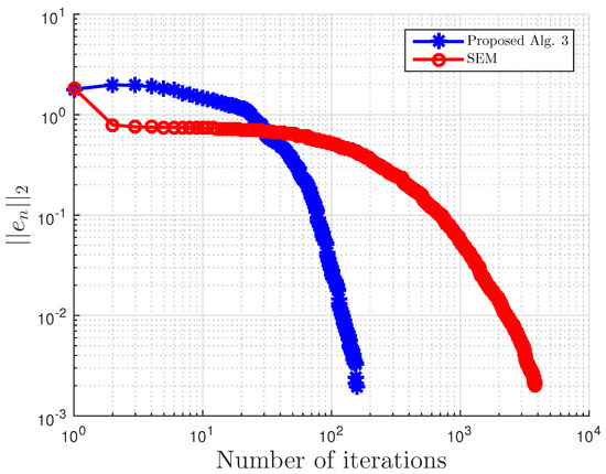
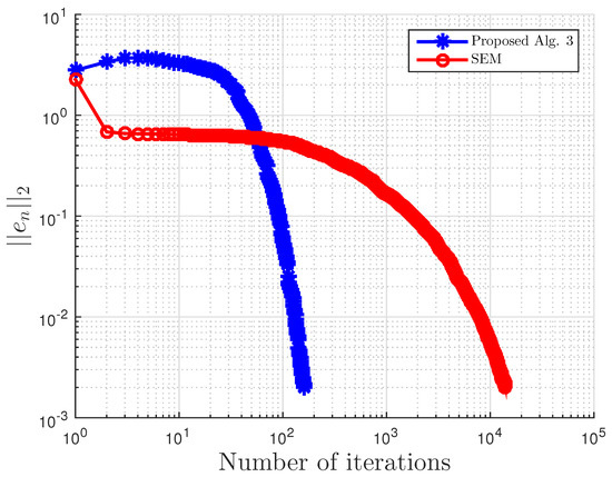
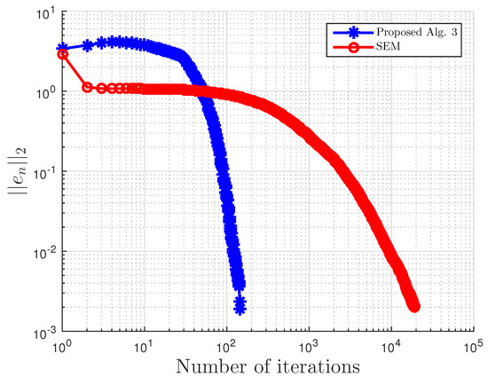
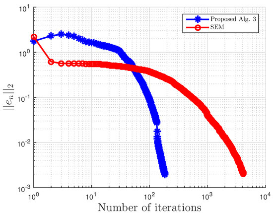
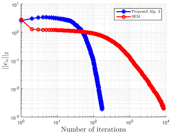
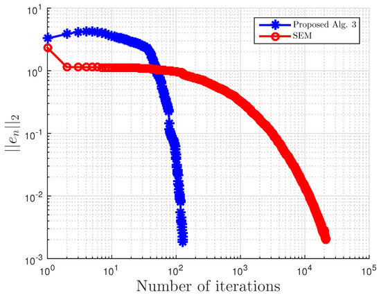
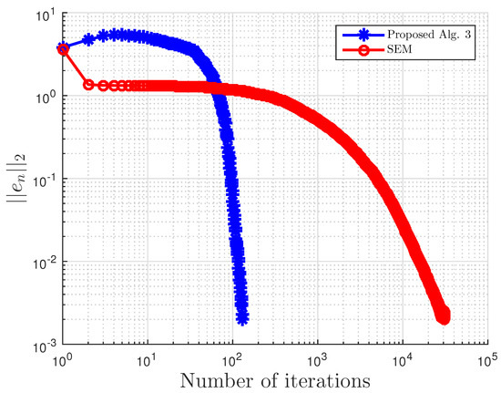
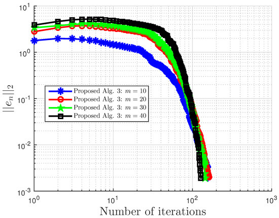
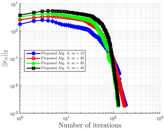
For this example, the stopping criterion is chosen as ${\parallel e_n\parallel }_2:={\parallel x_n\parallel }_2\le ϵ$, where $ϵ=0.002.$ We experiment with different values of k$(30,\mathrm{and}50)$ and m$(10,20,30,\mathrm{and}40)$. We randomly generate vector b and matrices B, S, and D. We choose ${\lambda }_0$ and μ appropriately in Algorithm 3. In (2), $L=\parallel M\parallel$ is used. Algorithm 3 proposed in this paper is compared with the subgradient-extragradient method (SEM) (2). For our proposed algorithm, we choose $\mu =0.999,$ ${\lambda }_0=0.5,$ and ${\alpha }_n=0.499$ while for SEM, $\lambda =\frac{0.125}{4L}.$ All results are reported in Table 5 and Figure 13, Figure 14, Figure 15, Figure 16, Figure 17, Figure 18, Figure 19, Figure 20, Figure 21 and Figure 22.

Table 5. Comparison of proposed Algorithm 3 and the subgradient-extragradient method (SEM) (2) for Example 3.

	$\mathit{m}=10$		$\mathit{m}=20$		$\mathit{m}=30$		$\mathit{m}=40$
$\mathit{k}=30$	Iter.	CPU Time	Iter.	CPU Time	Iter.	CPU Time	Iter.	CPU Time
Proposed Algorithm 3	157	2.7327	162	3.9759	144	4.4950	128	4.8193
SEM (2)	3785	64.8752	13,980	243.9019	18,994	345.3686	30,777	567.8440
	$\mathit{m}=\mathbf{10}$		$\mathit{m}=\mathbf{20}$		$\mathit{m}=\mathbf{30}$		$\mathit{m}=\mathbf{40}$
$\mathit{k}=\mathbf{50}$	Iter.	CPU Time	Iter.	CPU Time	Iter.	CPU Time	Iter.	CPU Time
Proposed Algorithm 3	185	4.0691	173	4.3798	128	4.8817	130	6.2658
SEM (2)	4176	77.6893	8645	150.4267	21,262	381.0991	30,956	561.4559

Figure 13. Example 3: $k=30$ and $m=10$.

Figure 14. Example 3: $k=30$ and $m=20$.

Figure 15. Example 3: $k=30$ and $m=30$.

Figure 16. Example 3: $k=30$ and $m=40$.

Figure 17. Example 3: $k=50$ and $m=10$.

Figure 18. Example 3: $k=50$ and $m=20$.

Figure 19. Example 3: $k=50$ and $m=30$.

Figure 20. Example 3: $k=50$ and $m=40$.

Figure 21. Example 3: $k=30$.

Figure 22. Example 3: $k=50$.

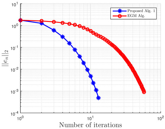
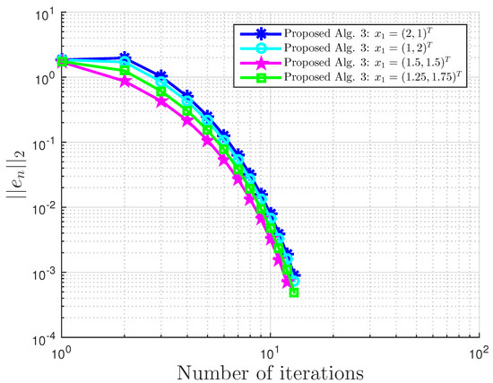
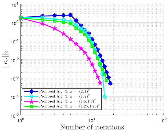
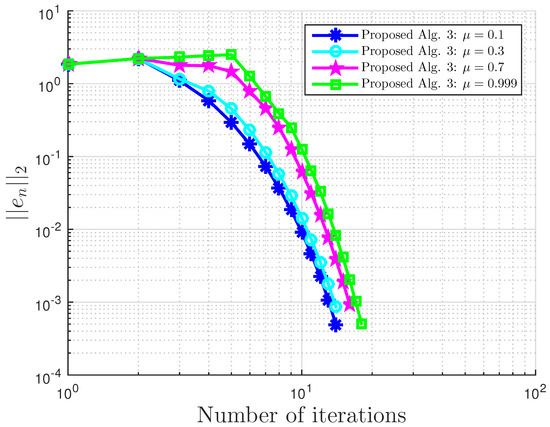
Example 4.

Consider VI(1) with:

$$\begin{array}{c}\hfill A\left(x\right)=\left(\begin{array}{c}0.5x_1{x}_2-2x_2-{10}^7\\ -4x_1+0.1x_2^2-{10}^7\end{array}\right)\end{array}$$

and:

$$C:=\{x\in {\mathbb{R}}^2:{(x_1-2)}^2+{(x_2-2)}^2\le 1\}.$$

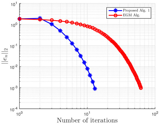
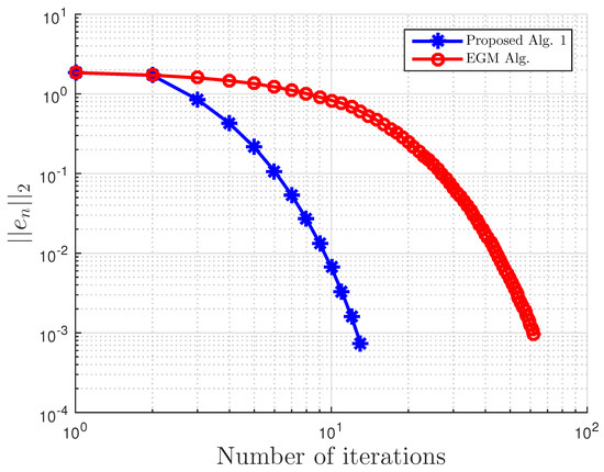
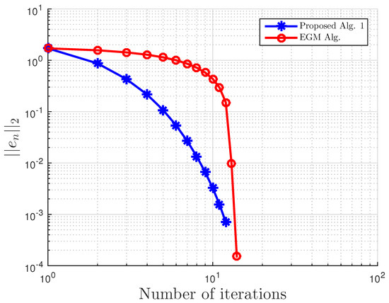
Then, A is not monotone on C, but pseudo-monotone. Furthermore, VI (1) has the unique solution $x^{*}={(2.707,2.707)}^T$. A comparison of our method is made with the extragradient method [16]. We denote the parameter in EGM [16] as ${\lambda }_n^{*}$ to differentiate it from ${\lambda }_n$ in our proposed Algorithm 3. We terminate the iterations if:

$${\parallel e_n\parallel }_2:={\parallel x_n-x^{*}\parallel }_2\le \epsilon$$

with $\epsilon ={10}^{-3}$. In this, our proposed Algorithm 3 is compared with the extragradient method (EGM) in [16]. For our proposed algorithm, we choose $x_0={(1,2)}^T$ and ${\alpha }_n=0.499$, while for EGM, ${\lambda }_n^{*}=0.00000001$. All results are reported in Table 6, Table 7 and Table 8 and Figure 23, Figure 24, Figure 25, Figure 26, Figure 27, Figure 28, Figure 29, Figure 30, Figure 31 and Figure 32.

Table 6. Comparison of proposed Algorithm 3 and the extragradient method (EGM) [16] for Example 4 with ${\lambda }_0=1$ and $\mu =0.1$.

	Proposed Algorithm 3		EGM [16]
${\mathit{x}}_1$	No. of Iter.	CPU Time	No. of Iter.	CPU Time
${(2,1)}^T$	13	$5.9390\times {10}^{-4}$	62	$1.8851\times {10}^{-3}$
${(1,2)}^T$	33	$5.2230\times {10}^{-4}$	62	$1.9666\times {10}^{-3}$
${(1.5,1.5)}^T$	12	$4.7790\times {10}^{-4}$	14	$3.955\times {10}^{-4}$
${(1.25,1.75)}^T$	13	$6.7980\times {10}^{-4}$	58	$1.9138\times {10}^{-3}$

Table 7. Proposed Algorithm 3 for Example 4 with ${\lambda }_0=5$ and $\mu =0.999$.

	Proposed Algorithm 3
${\mathit{x}}_1$	No. of Iter.	CPU Time
${(2,1)}^T$	18	$7.5980\times {10}^{-4}$
${(1,2)}^T$	15	$6.0910\times {10}^{-4}$
${(1.5,1.5)}^T$	13	$5.5840\times {10}^{-4}$
${(1.25,1.75)}^T$	16	$6.9110\times {10}^{-4}$

Table 8. Example 4: proposed Algorithm 3 with $x_1={(2,1)}^T$ for different $\mu$ and ${\lambda }_0$ values.

	${\mathit{\lambda }}_0=5$
	$\mathit{\mu }=\mathbf{0}.\mathbf{1}$	$\mathit{\mu }=\mathbf{0}.\mathbf{3}$	$\mathit{\mu }=\mathbf{0}.\mathbf{7}$	$\mathit{\mu }=\mathbf{0.999}$
No. of Iter.	14	14	16	18
CPU Time	$6.8600\times {10}^{-4}$	$7.1170\times {10}^{-4}$	$8.1080\times {10}^{-4}$	$8.6850\times {10}^{-4}$
	$\mathit{\mu }=\mathbf{0.999}$
	${\mathit{\lambda }}_{\mathbf{0}}=\mathbf{0}.\mathbf{1}$	${\mathit{\lambda }}_{\mathbf{0}}=\mathbf{1}$	${\mathit{\lambda }}_{\mathbf{0}}=\mathbf{5}$	${\mathit{\lambda }}_{\mathbf{0}}=\mathbf{10}$
No. of Iter.	12	18	18	18
CPU Time	$5.6360\times {10}^{-4}$	$9.3920\times {10}^{-4}$	$9.0230\times {10}^{-4}$	$8.9310\times {10}^{-4}$

Figure 23. Example 4: $k=50$ and $m=10$.

Figure 24. Example 4: $k=50$ and $m=20$.

Figure 25. Example 4: $k=50$ and $m=30$.

Figure 26. Example 4: $k=50$ and $m=40$.

Figure 27. Example 4: ${\lambda }_0=1$ and $\mu =0.1$.

Figure 28. Example 4: ${\lambda }_0=5$ and $\mu =0.999$.

Figure 29. Example 4: ${\lambda }_0=5$ and $x_1={(2,1)}^T$.

Figure 30. Example 4: $\mu =0.999$ and $x_1={(2,1)}^T$.

Figure 31. Example 5: ${\lambda }_0=1$, $\mu =0.9$ and $x_1=\frac{1}{12}(t^2-2t+1)$.

Figure 32. Example 5: ${\lambda }_0=1$, $\mu =0.9$ and $x_1=\frac{1}{9}{e}^{t}sin\left(t\right)$.

Example 5.

Consider $H:=L^2\left([0,1]\right)$ and $C:=\{x\in H:\parallel x\parallel \le 2\}$. Define $A:L^2\left([0,1]\right)\to L^2\left([0,1]\right)$ by:

$$A\left(u\right)\left(t\right):=e^{-{\parallel u\parallel }^2}{\int }_0^{t}u\left(s\right)ds,\forall u\in L^2\left([0,1]\right),t\in [0,1].$$

It can also be shown that A is pseudo-monotone, but not monotone on H, Lipschitz continuous with $L=\left(\frac{2}{e}+1\right)\frac{2}{\pi }$, and sequentially weakly-to-weak;y continuous on H (see Example 2.1 of [27]).

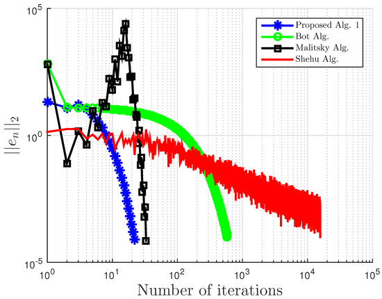
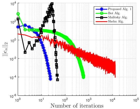
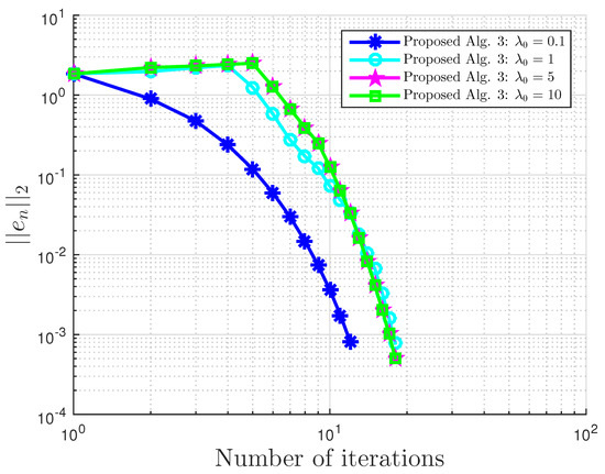
Our proposed Algorithm 3 is compared with Algorithm 1 proposed by Boţ et al. in [27] (Bot Alg.), Algorithm 2 proposed by Malitsky et al. in [28] (Malitsky Alg.), and Shehu and Iyiola’s proposed Algorithm 3.2 in [37] (Shehu Alg.). For our proposed algorithm, we choose $x_0=\frac{1}{9}{e}^{t}sin\left(t\right)$ and ${\alpha }_n=0.49,$ for Boţ et al., ${\rho }_n=0.02,$ for Malitsky et al., ${\theta }_0=1,$ and $\varphi =1.1$, while for Shehu and Iyiola, $\rho =1,$ $\sigma =0.005$, and $\gamma =0.9.$ All algorithms are terminated using the stopping criterion ${\parallel e_n\parallel }_2:={\parallel w_n-y_n\parallel }_2\le \epsilon$ with $\epsilon ={10}^{-4}$. All results are reported in Table 9 and Table 10 and Figure 33, Figure 34, Figure 35 and Figure 36.

Table 9. Example 5 comparison: proposed Algorithm 3, Bot Algorithm 1, Malitsky Algorithm 2, and Shehu Alg. [37] with ${\lambda }_0=1$ and $\mu =0.9$.

	Proposed Algorithm 3		Bot Algorithm 1		Malitsky Algorithm 2		Shehu Alg. [37]
${\mathit{x}}_1$	Iter.	CPU Time	Iter.	CPU Time	Iter.	CPU Time	Iter.	CPU Time
$\frac{1}{12}(t^2-2t+1)$	23	$5.1433\times {10}^{-3}$	2159	0.23341	371	$3.7625\times {10}^{-2}$	37,135	10.8377
$\frac{1}{9}{e}^{t}sin\left(t\right)$	18	$3.2111\times {10}^{-3}$	1681	0.18084	374	$3.9159\times {10}^{-2}$	70,741	32.5843
$\frac{1}{21}{t}^{2}cos\left(t\right)$	14	$2.4545\times {10}^{-3}$	4344	0.48573	373	$3.8413\times {10}^{-2}$	17,741	5.6272
$\frac{1}{7}(3t-2)e^t$	43	$8.7538\times {10}^{-3}$	2774	0.29515	351	$3.7544\times {10}^{-2}$	28,758	7.3424

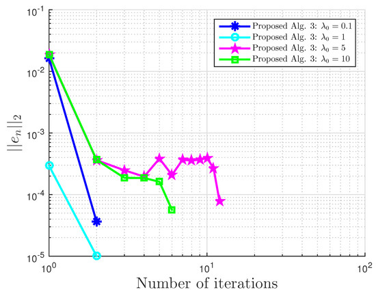
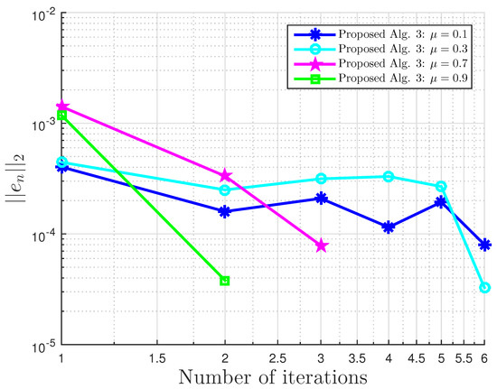
Table 10. Example 5: proposed Algorithm 3 with $x_1=\frac{t^2-2t+1}{12}$ for different $\mu$ and ${\lambda }_0$ values.

	$\mathit{\mu }=0.9$
	${\mathit{\lambda }}_{\mathbf{0}}=\mathbf{0}.\mathbf{1}$	${\mathit{\lambda }}_{\mathbf{0}}=\mathbf{1}$	${\mathit{\lambda }}_{\mathbf{0}}=\mathbf{2}$	${\mathit{\lambda }}_{\mathbf{0}}=\mathbf{3}$
No. of Iter.	167	23	11	8
CPU Time	$3.4828\times {10}^{-2}$	$4.2089\times {10}^{-3}$	$2.2288\times {10}^{-3}$	$1.3899\times {10}^{-3}$
	${\mathit{\lambda }}_{\mathbf{0}}=\mathbf{2}$
	$\mathit{\mu }=\mathbf{0}.\mathbf{1}$	$\mathit{\mu }=\mathbf{0}.\mathbf{3}$	$\mathit{\mu }=\mathbf{0}.\mathbf{7}$	$\mathit{\mu }=\mathbf{0}.\mathbf{999}$
No. of Iter.	11	11	11	11
CPU Time	$2.0615\times {10}^{-3}$	$2.1237\times {10}^{-3}$	$1.9886\times {10}^{-3}$	$2.0384\times {10}^{-3}$

Figure 33. Example 5: ${\lambda }_0=1$, $\mu =0.9$ and $x_1=\frac{1}{21}{t}^{2}cos\left(t\right)$.

Figure 34. Example 5: ${\lambda }_0=1$, $\mu =0.9$ and $x_1=\frac{1}{7}(3t-2)e^t$.

Figure 35. Example 5: $\mu =0.9$.

Figure 36. Example 5: ${\lambda }_0=2$.

5. Discussion

The weak convergence analysis of the reflected subgradient-extragradient method for variational inequalities in real Hilbert spaces is obtained in this paper. We provide and intensive numerical illustration and comparison with related works for several applications such as tomography reconstruction and Nash–Cournot oligopolistic equilibrium models. Our result is one of the few results on the subgradient-extragradient method with the reflected step in the literature. Our next project is to modify our results to bilevel variational inequalities.

References

- Fichera, G. Sul problema elastostatico di Signorini con ambigue condizioni al contorno. Atti Accad. Naz. Lincei VIII Ser. Rend. Cl. Sci. Fis. Mat. Nat. 1963, 34, 138–142. [Google Scholar]
- Fichera, G. Problemi elastostatici con vincoli unilaterali: Il problema di Signorini con ambigue condizioni al contorno. Atti Accad. Naz. Lincei Mem. Cl. Sci. Fis. Mat. Nat. Sez. I VIII Ser. 1964, 7, 91–140. [Google Scholar]
- Stampacchia, G. Formes bilineaires coercitives sur les ensembles convexes. C. R. Acad. Sci. 1964, 258, 4413–4416. [Google Scholar]
- Kinderlehrer, D.; Stampacchia, G. An Introduction to Variational Inequalities and Their Applications; Academic: New York, NY, USA, 1980. [Google Scholar]
- Facchinei, F.; Pang, J.S. Finite-Dimensional Variational Inequalities and Complementarity Problems. Volume I; Springer Series in Operations Research; Springer: New York, NY, USA, 2003. [Google Scholar]
- Facchinei, F.; Pang, J.S. Finite-Dimensional Variational Inequalities and Complementarity Problems. Volume II; Springer Series in Operations Research; Springer: New York, NY, USA, 2003. [Google Scholar]
- Konnov, I.V. Combined Relaxation Methods for Variational Inequalities; Springer: Berlin/Heidelberg, Germany, 2001. [Google Scholar]
- Iusem, A.N. An iterative algorithm for the variational inequality problem. Comput. Appl. Math. 1994, 13, 103–114. [Google Scholar]
- Iusem, A.N.; Svaiter, B.F. A variant of Korpelevich’s method for variational inequalities with a new search strategy. Optimization 1997, 42, 309–321. [Google Scholar] [CrossRef]
- Kanzow, C.; Shehu, Y. Strong convergence of a double projection-type method for monotone variational inequalities in Hilbert spaces. J. Fixed Point Theory Appl. 2018, 20, 51. [Google Scholar] [CrossRef]
- Khobotov, E.N. Modifications of the extragradient method for solving variational inequalities and certain optimization problems. USSR Comput. Math. Math. Phys. 1987, 27, 120–127. [Google Scholar] [CrossRef]
- Maingé, P.E. A hybrid extragradient-viscosity method for monotone operators and fixed point problems. SIAM J. Control Optim. 2008, 47, 1499–1515. [Google Scholar] [CrossRef]
- Marcotte, P. Application of Khobotov’s algorithm to variational inequalities and network equilibrium problems. Inf. Syst. Oper. Res. 1991, 29, 258–270. [Google Scholar] [CrossRef]
- Vuong, P.T. On the weak convergence of the extragradient method for solving pseudo-monotone variational inequalities. J. Optim. Theory Appl. 2018, 176, 399–409. [Google Scholar] [CrossRef]
- Shehu, Y.; Iyiola, O.S. Weak convergence for variational inequalities with inertial-type method. Appl. Anal. 2020, 2020, 1–25. [Google Scholar] [CrossRef]
- Korpelevich, G.M. The extragradient method for finding saddle points and other problems. Ekon. Matematicheskie Metody 1976, 12, 747–756. [Google Scholar]
- Antipin, A.S. On a method for convex programs using a symmetrical modification of the Lagrange function. Ekon. Matematicheskie Metody 1976, 12, 1164–1173. [Google Scholar]
- Censor, Y.; Gibali, A.; Reich, S. The subgradient-extragradient method for solving variational inequalities in Hilbert space. J. Optim. Theory Appl. 2011, 148, 318–335. [Google Scholar] [CrossRef]
- Censor, Y.; Gibali, A.; Reich, S. Strong convergence of subgradient-extragradient methods for the variational inequality problem in Hilbert space. Optim. Methods Softw. 2011, 26, 827–845. [Google Scholar] [CrossRef]
- Censor, Y.; Gibali, A.; Reich, S. Extensions of Korpelevich’s extragradient method for the variational inequality problem in Euclidean space. Optimization 2011, 61, 1119–1132. [Google Scholar] [CrossRef]
- Malitsky, Y.V. Projected reflected gradient methods for monotone variational inequalities. SIAM J. Optim. 2015, 25, 502–520. [Google Scholar] [CrossRef]
- Malitsky, Y.V.; Semenov, V.V. A hybrid method without extrapolation step for solving variational inequality problems. J. Glob. Optim. 2015, 61, 193–202. [Google Scholar] [CrossRef]
- Solodov, M.V.; Svaiter, B.F. A new projection method for variational inequality problems. SIAM J. Control Optim. 1999, 37, 765–776. [Google Scholar] [CrossRef]
- Denisov, S.V.; Semenov, V.V.; Chabak, L.M. Convergence of the modified extragradient method for variational inequalities with non-Lipschitz operators. Cybern. Syst. Anal. 2015, 51, 757–765. [Google Scholar] [CrossRef]
- Yang, J.; Liu, H. Strong convergence result for solving monotone variational inequalities in Hilbert space. Numer. Algorithms 2019, 80, 741–752. [Google Scholar] [CrossRef]
- Thong, D.V.; Hieu, D.V. Modified subgradient-extragradient method for variational inequality problems. Numer. Algorithms 2018, 79, 597–610. [Google Scholar] [CrossRef]
- Boţ, R.I.; Csetnek, E.R.; Vuong, P.T. The forward-backward-forward method from discrete and continuous perspective for pseudomonotone variational inequalities in Hilbert spaces. Eur. J. Oper. Res. 2020, 287, 49–60. [Google Scholar] [CrossRef]
- Malitsky, Y.V. Golden ratio algorithms for variational inequalities. Math. Program. 2020, 184, 383–410. [Google Scholar] [CrossRef]
- Karamardian, S. Complementarity problems over cones with monotone and pseudo-monotone maps. J. Optim. Theory Appl. 1976, 18, 445–454. [Google Scholar] [CrossRef]
- Goebel, K.; Reich, S. Uniform Convexity, Hyperbolic Geometry, and Nonexpansive Mappings; Marcel Dekker: New York, NY, USA, 1984. [Google Scholar]
- Kopecká, E.; Reich, S. A note on alternating projections in Hilbert spaces. J. Fixed Point Theory Appl. 2012, 12, 41–47. [Google Scholar] [CrossRef]
- Cegielski, A. Iterative Methods for Fixed Point Problems in Hilbert Spaces; Lecture Notes in Mathematics; Springer: Berlin/Heidelberg, Germany, 2012. [Google Scholar]
- Cottle, R.W.; Yao, J.C. Pseudo-monotone complementarity problems in Hilbert space. J. Optim. Theory Appl. 1992, 75, 281–295. [Google Scholar] [CrossRef]
- Opial, Z. Weak convergence of the sequence of successive approximations for nonexpansive mappings. Bull. Am. Math. Soc. 1967, 73, 591–597. [Google Scholar] [CrossRef]
- He, Y.R. A new double projection algorithm for variational inequalities. J. Comput. Appl. Math. 2006, 185, 166–173. [Google Scholar] [CrossRef]
- Maingé, P.E. Convergence theorems for inertial KM-type algorithms. J. Comput. Appl. Math. 2008, 219, 223–236. [Google Scholar] [CrossRef]
- Shehu, Y.; Iyiola, O.S. Iterative algorithms for solving fixed point problems and variational inequalities with uniformly continuous monotone operators. Numer. Algorithms 2018, 79, 529–553. [Google Scholar] [CrossRef]
- Yen, L.H.; Muu, L.D.; Huyen, N.T.T. An algorithm for a class of split feasibility problems: Application to a model in electricity production. Math. Methods Oper. Res. 2016, 84, 549–565. [Google Scholar] [CrossRef]
- Harker, P.T.; Pang, J.-S. A damped-Newton method for the linear complementarity problem. In Computational Solution of Nonlinear Systems of Equations, Lectures in Applied Mathematics; Allgower, G., Georg, K., Eds.; AMS: Providence, RI, USA, 1990; Volume 26, pp. 265–284. [Google Scholar]
Publisher’s Note: MDPI stays neutral with regard to jurisdictional claims in published maps and institutional affiliations. |
© 2021 by the authors. Licensee MDPI, Basel, Switzerland. This article is an open access article distributed under the terms and conditions of the Creative Commons Attribution (CC BY) license (http://creativecommons.org/licenses/by/4.0/).