Homotopic Parametric Continuation Method for Determining Stationary States of Chemical Reactors with Dispersion

Abstract

Physical processes occurring in devices with distributed variables and a turbulent tide with a dispersion of mass and heat are often modeled using systems of nonlinear equations. Solving such a system is sometimes impossible in an analytical manner. The iterative methods, such as Newton’s method, are not always sufficiently effective in such cases. In this article, a combination of the homotopy method and the parametric continuation method was proposed to solve the system of nonlinear differential equations. These methods are symmetrical, i.e., the calculations can be made by increasing or decreasing the value of the parameters. Thanks to this approach, the determination of all roots of the system does not require any iterative method. Moreover, when the solutions of the system are close to each other, the proposed method easily determines all of them. As an example of the method use a mathematical model of a non-adiabatic catalytic pseudohomogeneous tubular chemical reactor with longitudinal dispersion was chosen.

1. Introduction

Physical processes and phenomena occurring in devices with distributed variables and a turbulent tide with a dispersion of mass and heat are modeled using systems of differential equations. For stationary states, these are Ordinary Differential Equations (ODE’s). Examples of such apparatuses are tubular chemical reactors with longitudinal dispersion. Systems of ordinary differential equations of the second order are used to describe them [1]. The analytical solution of these equations is impossible due to their non-linearity. Therefore, various types of numerical methods are used to determine stationary solutions of such systems [2,3]. However, not every numerical method is useful and effective; for example, Newton’s iterative method is completely useless when there are so-called multiple stationary states [1]. Determining all states (all solutions) using Newton’s method is practically impossible, especially when these states are located close to each other and there are many of them.

One of the numerical methods that allow for easy determination of all stationary solutions of the system of nonlinear equations is the parametric continuation method. This method does not require any iteration procedures. Moreover, this method allows obtaining a solution by increasing or decreasing the parameter value. For this reason, it can be considered a symmetrical method. It was used, among others, in [1], where the stationary states of the reactor were determined in the given range of the variability of selected control parameters of the apparatus.

If the task is not to determine the stationary states of the reactor in a given range of variability of the control parameter, but the task is to determine these states for the set values of all parameters of the apparatus, then the combination of the parametric continuation method with the homotopy method is perfect. Its idea is to construct a special function dependent on an additional parameter p in such a way that with a continuous change of the value of this parameter from $p=0$, we get all the solutions for $p=1$. In the event that these solutions are ambiguous, the homotopy curve must pass through $p=1$ many times. This means that the curve is then a hysteresis loop, as shown in the corresponding graphs in this paper.

Studies using the homotopy method can be found in the scientific literature, for example, articles [4,5,6,7,8,9,10,11,12,13,14]. However, the parametric continuation method, as used in this paper, was not used there. The method used in the cited literature consists of changing the homotopy parameter p by the assumed increase in $\Delta p$. Then, at each step, the system of equations is solved iteratively using Newton’s method. This is quite inconvenient for two reasons. The first is that iterating the equations at each step significantly increases the computation time. The second, more important, reason is that this method is useless when the system of equations has an ambiguous solution, i.e., it has many roots [11]. The search for each of them is associated with a change of initial values. The homotopy curve must then turn around several times. This means that the increment of $\Delta p$ must change the sign. However, it is difficult to predict when this sign should be changed. The parametric continuation method used in this work is devoid of all these drawbacks. This method has also been described and used in [1,15]. This is described in detail later in this paper.

As an example of the application of the described method, the mathematical model of a non-adiabatic catalytic pseudohomogeneous tubular chemical reactor with longitudinal dispersion was taken. Such a reactor is described by a system of second-order ordinary differential equations with appropriate boundary conditions.

This article is structured as follows. The subject of the work was outlined in the first part. The second part describes the mathematical foundations of the discussed methods. The following sections describe the chemical reactor model and present the results. The last part is the Conclusions.

2. Mathematical Foundations of the Method

The problem concerns the determination of solutions to the following system of equations:

$$\underline{f}\left(\underline{x}\right)=\underline{0}.$$

(1)

Assuming that for $p=0$ $\underline{x}=\underline{x^{*}}$, then the homotopy function takes the form:

$$\underline{F}(\underline{x},p)=\underline{f}\left(\underline{x}\right)+(p-1)\underline{f}\left(\underline{x^{*}}\right)=\underline{0},$$

(2)

where $\underline{x^{*}}$ is any vector, it is obvious that the searched solutions of Equation (1) are found only on the $p=1$ line. To get to this line, Equation (2) should be carried out from point $\underline{x^{*}}$ for $p=0$ to point $\underline{x}$ for $p=1$, which are solutions of the system of Equations (1).

The following parametric continuation method can be used for this purpose:

$$\underline{x_{k+1}}=\underline{x_k}-\underline{\underline{J_k^{-1}}}\underline{w_k}\Delta psign(det\underline{\underline{J_k}}),$$

(3)

$$p_{k+1}=p_k+\Delta psign(det\underline{\underline{J_k}}),$$

(4)

where:

$$\begin{array}{c}\underline{x}=\left\{x_j\right\},\end{array}$$

(5)

$$\begin{array}{c}\underline{\underline{J_{}}}=\left\{\frac{\partial f_i}{\partial x_j}\right\},\end{array}$$

(6)

$$\begin{array}{c}\underline{w}=\left\{f_i\left(\underline{x^{*}}\right)\right\}=const.\end{array}$$

(7)

The sign of the determinant of the Jacobi matrix, $sign(det\underline{\underline{J_k}})$, indicates the direction of changes in the homotopy parameter p.

3. Determination of the Solutions of the Chemical Reactor Model

The method presented above was used to determine the stationary states of a non-adiabatic catalytic tubular chemical reactor with longitudinal dispersion. The model assumes that the gas temperature is equal to the catalyst temperature. This means that we are dealing then with a pseudohomogeneous reactor. Assuming that a single chemical reaction takes place in the reactor, the mathematical model of such an apparatus is written in the form of two second-order differential equations:

Mass balance:

$$\frac{\mathrm{d}\alpha }{\mathrm{d}z}=\frac{1}{P{e}_M}\frac{{\mathrm{d}}^2\alpha }{\mathrm{d}{z}^2}+{\Phi }_1\left(\alpha ,\Theta \right),$$

(8)

Heat balance:

$$\frac{\mathrm{d}\Theta }{\mathrm{d}z}=\frac{1}{P{e}_H}\frac{{\mathrm{d}}^2\Theta }{\mathrm{d}{z}^2}+{\Phi }_2\left(\alpha ,\Theta \right),$$

(9)

where $0\le z\le 1$.

The following boundary conditions are associated with the above equations:

$$\begin{array}{c}\alpha \left(0\right)=\frac{1}{P{e}_M}{\frac{\mathrm{d}\alpha }{\mathrm{d}z}}_{z=0},\end{array}$$

(10)

$$\begin{array}{c}{\frac{\mathrm{d}\alpha }{\mathrm{d}z}}_{z=1}=0,\end{array}$$

(11)

$$\begin{array}{c}\Theta \left(0\right)=\frac{1}{P{e}_H}{\frac{\mathrm{d}\Theta }{\mathrm{d}z}}_{z=0},\end{array}$$

(12)

$$\begin{array}{c}{\frac{\mathrm{d}\Theta }{\mathrm{d}z}}_{z=1}=0.\end{array}$$

(13)

Assuming that a single $A\to B$ type reaction takes place in the reactor, the functions related to reaction kinetics and heat transfer are as follows:

$$\begin{array}{c}{\Phi }_1=Da{(1-\alpha )}^{n}exp\left\{\left(\gamma \frac{\Theta }{\beta +\Theta }\right)\right\},\end{array}$$

(14)

$$\begin{array}{c}{\Phi }_2=\beta {\Phi }_1+\delta ({\Theta }_H-\Theta ).\end{array}$$

(15)

By introducing additional variable definitions:

$$\begin{array}{c}{u}_1=\alpha ,\end{array}$$

(16)

$$\begin{array}{c}{u}_2=\frac{\mathrm{d}\alpha }{\mathrm{d}z},\end{array}$$

(17)

and:

$$\begin{array}{c}{v}_1=\Theta ,\end{array}$$

(18)

$$\begin{array}{c}{v}_2=\frac{\mathrm{d}\Theta }{\mathrm{d}z},\end{array}$$

(19)

a system of four first-order differential equations is obtained:

$$\begin{array}{c}\frac{\mathrm{d}{u}_1}{\mathrm{d}z}=u_2,\end{array}$$

(20)

$$\begin{array}{c}\frac{\mathrm{d}{u}_2}{\mathrm{d}z}=P{e}_M{u}_2-{\Phi }_1(u_1,v_1),\end{array}$$

(21)

$$\begin{array}{c}\frac{\mathrm{d}{v}_1}{\mathrm{d}z}=v_2,\end{array}$$

(22)

$$\begin{array}{c}\frac{\mathrm{d}{v}_2}{\mathrm{d}z}=P{e}_H{v}_2-{\Phi }_2(u_1,v_1),\end{array}$$

(23)

with the appropriate boundary conditions:

$$\begin{array}{c}P{e}_M{u}_1\left(0\right)-u_2\left(0\right)=0,\end{array}$$

(24)

$$\begin{array}{c}{u}_2\left(1\right)=0,\end{array}$$

(25)

$$\begin{array}{c}P{e}_H{v}_1\left(0\right)-v_2\left(0\right)=0,\end{array}$$

(26)

$$\begin{array}{c}{v}_2\left(1\right)=0.\end{array}$$

(27)

It can be shown that the forward integration of the above equations (i.e., from $z=0$ to $z=1$) is numerically unstable. The integration, therefore, has to go backwards (from $z=1$ to $z=0$). The initial values for this integration will, therefore, be: $u_1\left(1\right)$ and $v_1\left(1\right)$, as well as $u_2\left(1\right)=0$ and $v_2\left(1\right)=0$. According to Equation (2), the individual functions of the homotopy can be defined based on the boundary conditions in Equations (24) and (26) as follows:

$$\begin{array}{c}{F}_1[u_1\left(1\right),v_1\left(1\right)]=P{e}_M{u}_1\left(0\right)-u_2\left(0\right)+(p-1)[P{e}_M{u}_1^{*}\left(0\right)-u_2^{*}\left(0\right)]=0,\end{array}$$

(28)

$$\begin{array}{c}{F}_2[u_1\left(1\right),v_1\left(1\right)]=P{e}_H{v}_1\left(0\right)-v_2\left(0\right)+(p-1)[P{e}_H{v}_1^{*}\left(0\right)-v_2^{*}\left(0\right)]=0.\end{array}$$

(29)

The parametric continuation procedure, therefore, takes the following form:

$$\left[\begin{array}{c}{u}_{1,k+1}\left(1\right)\\ v_{1,k+1}\left(1\right)\end{array}\right]=\left[\begin{array}{c}{u}_{1,k}\left(1\right)\\ v_{1,k}\left(1\right)\end{array}\right]-\underline{\underline{J_k^{-1}}}\underline{w_k}\Delta psign(det\underline{\underline{J_k}}),$$

(30)

$$\begin{array}{c}{p}_{k+1}=p_k+\Delta psign(det\underline{\underline{J_k}}),\end{array}$$

(31)

where:

$$\begin{array}{c}\underline{\underline{J_{}}}=\left[\begin{array}{cc}\frac{\partial F_1}{\partial u_1\left(1\right)}& \frac{\partial F_1}{\partial v_1\left(1\right)}\\ \frac{\partial F_2}{\partial u_1\left(1\right)}& \frac{\partial F_2}{\partial v_1\left(1\right)}\end{array}\right],\end{array}$$

(32)

$$\begin{array}{c}\underline{w}=\left[\begin{array}{c}P{e}_M{u}_1^{*}\left(0\right)-u_2^{*}\left(0\right)\\ P{e}_H{v}_1^{*}\left(0\right)-v_2^{*}\left(0\right)\end{array}\right]=const.\end{array}$$

(33)

The adopted calculation method is as follows. Any values of $u_1^{*}\left(1\right)$ and $v_1^{*}\left(1\right)$ and $u_2^{*}\left(1\right)=0$ and $v_2^{*}\left(1\right)=0$ are assumed. As a result of one-time integration of Equations (20)–(23), $u_1^{*}\left(0\right)$ and $v_1^{*}\left(0\right)$ are obtained, which are then used in Equations (28) and (29). These values are constant for the entire calculation process. At the same time, these are the initial values for the continuation procedure, i.e., $u_{1,0}\left(1\right)=u_1^{*}\left(1\right)$ and $v_{1,0}\left(1\right)=v_1^{*}\left(1\right)$. The searched solutions of the reactor model lie on the $p=1$ line. The partial derivatives in the Jacobi matrix, Equation (32), should be determined numerically.

4. Calculation Results

Depending on the values of the model parameters, the reactor has single or multiple stationary states. In this study, these parameters were selected so that the reactor was characterized by more complex solutions, i.e., three states. For example, the following values of the reactor model parameters were adopted: $\gamma =14,\beta =2,n=1.7,P{e}_M=200,P{e}_H=100,Da=0.0435,\delta =3,{\Theta }_H=-0.05$. The results of the calculations are shown in Figure 1. As this figure shows, the tested reactor model has three different solutions, which should be read for $p=1$. This means that the reactor has three different stationary states. It should be noted that for different values of $u_1^{*}\left(1\right)$ and $v_1^{*}\left(1\right)$, a different homotopy curve is obtained. However, they must all intersect at the same point on the line $p=1$.

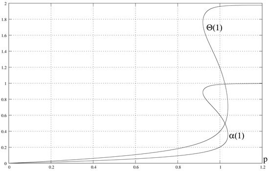
Figure 1. For the assumed parameters, the reactor has three different stationary states.

5. Discussion

Various known numerical methods can be used to solve systems of equations in the form of Equation (1). The simplest of them are iterative methods, which include, e.g., Newton’s method or the Chun-Hui He method [16]. However, these methods require a lot of iterations and thus use a lot of computer time to get the final solutions. Thus, their use becomes ineffective. Moreover, iterative methods cannot cope when the system has ambiguous (multiple) solutions (see Figure 3 in [17]). The approach proposed in this paper is devoid of the above drawbacks.

As for the homotope method, it requires a series of calculations for each value of the p parameter separately. Iterative methods are also used for these calculations, the same as described in the previous paragraph. This approach is, therefore, also numerically time-consuming. It requires many iterative calculations to obtain the final solution. Modifications of the homotope method known from the literature, such as the perturbative homotopy method [18], do not solve this problem. Only using the homotopy method in conjunction with the parametric continuation method causes the final solution to be obtained immediately, regardless of the number of multiple stationary states. Instead of looking for solutions for Equation (2) for successive values of the p parameter, the solution is obtained step by step from Equations (3) and (4). Thus, there is no need to perform any additional iterative calculations.

6. Conclusions

The presented work presents the homotopy method for determining the solutions of the mathematical model of a non-adiabatic catalytic pseudohomogeneous tubular chemical reactor with longitudinal dispersion. Such a model is written by means of second-order differential equations with boundary conditions. The solutions sought are the stationary states of the reactor. The proposed method consists of carrying out homotopy F functions from the homotopy parameter $p=0$ and further along the lines determining the zeroing of these functions. These lines can be obtained using the parametric continuation method. The advantage of this approach is that the determination of the partial derivatives of the function F with respect to the parameter takes place only once for the entire computational process. These derivatives are stored permanently in the vector $\underline{w}$ (Formula ()). The whole computational process does not require any iteration, and all the searched elements are found in one computational process. All this significantly speeds up the calculations and, above all, makes it possible to determine all the elements easily.

According to the homotopy principle, the searched solutions lie only on the $p=1$ line. As a result of the exemplary calculations, the graphs in Figure 1 were obtained. These graphs show that the tested reactor has three different stationary states.

References

- Berezowski, M. The application of the parametric continuation method for determining steady state diagrams in chemical engineering. Chem. Eng. Sci. 2010, 65, 5411–5414. [Google Scholar] [CrossRef] [Green Version]
- Guran, L.; Mitrović, Z.D.; Reddy, G.S.M.; Belhenniche, A.; Radenović, S. Applications of a Fixed Point Result for Solving Nonlinear Fractional and Integral Differential Equations. Fractal Fract. 2021, 5, 211. [Google Scholar] [CrossRef]
- Younis, M.; Fabiano, N.; Fadail, Z.M.; Mitrović, Z.D.; Radenović, S. Some new observations on fixed point results in rectangular metric spaces with applications to chemical sciences. Vojnoteh. Glas./Mil. Tech. Cour. 2021, 69, 8–30. [Google Scholar] [CrossRef]
- Baayen, J.; Becker, B.; van Heeringen, K.J.; Miltenburg, I.; Piovesan, T.; Rauw, J.; den Toom, M.; VanderWees, J. An overview of continuation methods for non-linear model predictive control of water systems. IFAC-PapersOnLine 2019, 52, 73–80. [Google Scholar] [CrossRef]
- Brown, D.A.; Zingg, D.W. Monolithic homotopy continuation with predictor based on higher derivatives. J. Comput. Appl. Math. 2019, 346, 26–41. [Google Scholar] [CrossRef]
- Gallardo-Alvarado, J. An Application of the Newton–Homotopy Continuation Method for Solving the Forward Kinematic Problem of the 3-<u>R</u>RS Parallel Manipulator. Math. Probl. Eng. 2019, 2019, 3123808. [Google Scholar] [CrossRef]
- Gritton, K.S.; Seader, J.; Lin, W.J. Global homotopy continuation procedures for seeking all roots of a nonlinear equation. Comput. Chem. Eng. 2001, 25, 1003–1019. [Google Scholar] [CrossRef]
- Jiménez-Islas, H.; Martínez-González, G.M.; Navarrete-Bolaños, J.L.; Botello-Álvarez, J.E.; Oliveros-Muñoz, J.M. Nonlinear Homotopic Continuation Methods: A Chemical Engineering Perspective Review. Ind. Eng. Chem. Res. 2013, 52, 14729–14742. [Google Scholar] [CrossRef]
- Jiménez-Islas, H.; Calderón-Ramírez, M.; Martínez-González, G.M.; Calderón-Álvarado, M.P.; Oliveros-Muñoz, J.M. Multiple solutions for steady differential equations via hyperspherical path-tracking of homotopy curves. Comput. Math. Appl. 2020, 79, 2216–2239. [Google Scholar] [CrossRef]
- Pan, B.; Ma, Y.; Ni, Y. A new fractional homotopy method for solving nonlinear optimal control problems. Acta Astronaut. 2019, 161, 12–23. [Google Scholar] [CrossRef]
- Rahimian, S.K.; Jalali, F.; Seader, J.; White, R. A new homotopy for seeking all real roots of a nonlinear equation. Comput. Chem. Eng. 2011, 35, 403–411. [Google Scholar] [CrossRef]
- Słota, D.; Chmielowska, A.; Brociek, R.; Szczygieł, M. Application of the Homotopy Method for Fractional Inverse Stefan Problem. Energies 2020, 13, 5474. [Google Scholar] [CrossRef]
- Wang, Y.; Topputo, F. A Homotopy Method Based on Theory of Functional Connections. 2020. Available online: https://arxiv.org/pdf/1911.04899.pdf (accessed on 27 November 2021).
- Wayburn, T.; Seader, J. Homotopy continuation methods for computer-aided process design. Comput. Chem. Eng. 1987, 11, 7–25. [Google Scholar] [CrossRef]
- Berezowski, M. Determination of catastrophic sets of a tubular chemical reactor by two-parameter continuation method. Int. J. Chem. React. Eng. 2020, 18, 20200135. [Google Scholar] [CrossRef]
- Khan, W.A. Numerical simulation of Chun-Hui He’s iteration method with applications in engineering. Int. J. Numer. Methods Heat Fluid Flow 2021. ahead-of-print. [Google Scholar] [CrossRef]
- Berezowski, M. Method of determination of steady-state diagrams of chemical reactors. Chem. Eng. Sci. 2000, 55, 4291–4295. [Google Scholar] [CrossRef]
- He, J.H. Comparison of homotopy perturbation method and homotopy analysis method. Appl. Math. Comput. 2004, 156, 527–539. [Google Scholar] [CrossRef]
Publisher’s Note: MDPI stays neutral with regard to jurisdictional claims in published maps and institutional affiliations. |
© 2021 by the authors. Licensee MDPI, Basel, Switzerland. This article is an open access article distributed under the terms and conditions of the Creative Commons Attribution (CC BY) license (https://creativecommons.org/licenses/by/4.0/).