Exact Closed-Form Solutions of the Motion in Non-Inertial Reference Frames, Using the Properties of Lie Groups SO₃ and SE₃

Abstract

The paper offers a general symbolic method to study the motion in a non-inertial reference frame. In order to achieve this, we use the algebraic and geometric properties of the Lie group of special orthogonal tensors, ${\mathbf{SO}}_3$, and the Lie group of the rigid body displacements, ${\mathbf{SE}}_3$. We obtain a simplified form of the initial value problem that models the non-inertial motion using a tensor instrument introduced in this paper. Thus, the study of the motion in a non-inertial reference frame is transferred into the study of a classical motion in an inertial reference frame. The applications of this method refer to solving the relative motion problem and deriving the straightforward solution to classical theoretical mechanics problems. The motion in a uniform gravitational force field in a rotating reference frame, the motion of a charged particle in non-stationary electric and magnetic fields, the exact solution of the relative rigid body motion in the non-inertial reference frame are studied. Using this symbolic method in studying the motion in a non-inertial reference frame reduces the number of computations. In addition, it offers, in some essential particular cases, exact closed-form coordinate-free analytical solutions.

1. Introduction

The motion in a non-inertial reference frame and in electric and magnetic fields are important tools, both in theoretical problems and practical applications. The present approach offers a new general method to study these aspects. Even though the problems discussed in the paper can be found in classical mechanics textbooks [1,2,3,4,5,6,7,8,9,10,11,12,13,14,15,16,17,18,19,20], they were never solved in all their general aspects. The symbolic tensor instrument presented in this paper simplifies the complex initial value problem that models the motion in a non-inertial reference frame, and was introduced in Reference [21]. It was used to approach several classical and celestial mechanics problems, such as: the Kepler problem in a rotating reference frame [22,23], the Foucault Pendulum-like problem [24], and the spacecraft relative orbital motion problem [25,26,27,28]. The tensor operator is introduced by the Poisson-Darboux equation [29], written in its tensor form [21,22,23,30]. In most situations discussed here, this operator has a closed-form time-explicit formula. It allows to determine explicit or closed form coordinate-free expressions for the relative law of motion and the relative velocity. The motion of a mass particle in a uniform gravitational field in a rotating reference frame, the motion of a charged particle in non-stationary electric and magnetic fields, and the exact solution of the relative rigid body motion in a non-inertial reference frame are studied. The result displayed in Theorems 11 and 12 gives significant insight into the motion of any rigid body with respect to a non-inertial reference frame. A straightforward method to approach its motion is revealed as follows:

(i)

The problem is solved in an inertial frame, that is, our non-inertial frame “frozen” at the initial moment.

(ii)

The solution to the non-inertial problem is obtained by applying a well-defined orthogonal tensor to the solution obtained at the previous step (i).

The core result of the paper offers a meaningful understanding and a natural geometrical interpretation of the motion in a non-inertial reference frame.

The paper is structured as follows: in the second section, a tensor map and a differentiation operator, along with some of their properties, are introduced. In the third section, based on the mathematical instruments previously discussed, we give exact closed-form solutions to two particular types of initial value problems. For each of them, two equivalent solutions are offered. Using these mathematical results, in the fourth and fifth section, we analyze the motion of a mass particle in a uniform gravitational field with respect to a non-inertial reference frame and the motion of a charged particle in non-stationary electric and magnetic fields, respectively. In the sixth section, the motion of a rigid body with respect to a non-inertial reference frame is studied, and an exact closed-form solution is given for this motion. The last section presents the conclusions.

2. Tensorial Considerations

This section introduces the main mathematical instruments used in this paper [31,32]. A tensor map and a vector differential operator will be defined. The following notations are introduced:

• t the time variable;
• $\frac{\mathrm{d}}{\mathrm{d}t}( )=\stackrel{·}{( )}$ the derivative with respect to time;
• ${\mathbf{V}}_3$ the set of free vectors in the three dimensional Euclidean space;
• ${\mathbf{V}}_3^{ℝ}$ the set of functions of real variable, with values in ${\mathbf{V}}_3$;
• ${\mathbf{V}}_3^{{ℝ}_{+}}$ the set of functions of real positive variable, with values in ${\mathbf{V}}_3$;
• ${\mathbf{R}}^T$ the transpose of tensor $\mathbf{R}$;
• ${\mathbf{SO}}_3$ the special orthogonal group of second order tensors:

  $${\mathbf{SO}}_3= \left\{\mathbf{Q}|\mathbf{Q}{\mathbf{Q}}^T=I_3,\hspace{0.33em}\det (\mathbf{Q})=1\right\};$$
• ${\mathbf{SO}}_3^{ℝ}$ the set of functions of real variable, with values in ${\mathbf{SO}}_3$;
• $\tilde{\omega }$ the skew-symmetric tensor associated with the vector $\mathbf{\omega }$;
• ${\mathbf{so}}_3$ the Lie-algebra of skew-symmetric second order tensors:

  $${\mathbf{so}}_3= \left\{\tilde{\omega }|{\tilde{\omega }}^T=-\tilde{\omega }\right\};$$
• ${\mathbf{so}}_3^{ℝ}$ the set of functions of real variable, with values in ${\mathbf{so}}_3$;
• ${\mathbf{so}}_3^{{ℝ}_{+}}$ the set of functions of real positive variable, with values in ${\mathbf{so}}_3$.

2.1. A Tensor Operator

The rotation with arbitrary angular velocity ω is related to proper orthogonal tensor maps of real variable by a tensor initial value problem (IVP), similar to the one from attitude kinematics, which is also referred to as the Poisson-Darboux equation [30,33].

Lemma 1. 

Consider the IVP:

$$\stackrel{.}{\mathbf{Q}}=\mathbf{Q}\tilde{\omega };\hspace{0.33em}\hspace{0.33em}\mathbf{Q}(t_0)=I_3,\hspace{0.33em}\hspace{0.33em}{t}_0\ge 0.$$

(1)

For any continuous map$\tilde{\omega }\in \mathrm{s}{\mathbf{o}}_3^{ℝ}$, there exists a unique solution$\mathbf{Q}\in \mathrm{S}{\mathbf{O}}_3^{ℝ}$  of the problem.

Proof. 

From the existence and uniqueness theorem, it follows that the IVP (1) has a unique solution $\mathbf{Q}=\mathbf{Q}(t)$. One has to prove that Q is in ${\mathbf{SO}}_3^{ℝ}$, meaning that ${\mathbf{Q}}^T\mathbf{Q}=I_3$. We may write $\frac{\mathrm{d}}{\mathrm{d}t}(\mathbf{Q}{\mathbf{Q}}^T)=\stackrel{.}{\mathbf{Q}}{\mathbf{Q}}^T+\mathbf{Q}{\stackrel{.}{\mathbf{Q}}}^T=\mathbf{Q}\tilde{\omega }{\mathbf{Q}}^T-\mathbf{Q}\tilde{\omega }{\mathbf{Q}}^T=0_3$; hence, $\mathbf{Q}{\mathbf{Q}}^T$ is a constant differentiable function that satisfies $(\mathbf{Q}{\mathbf{Q}}^T)(t_0)={\mathbf{I}}_3$. It follows that $\mathbf{Q}{\mathbf{Q}}^T={\mathbf{I}}_3$. Since $\det (\mathbf{Q})$ is also a continuous function which satisfies $\det (\mathbf{Q})\in \{-1,1\}$ and $\det (\mathbf{Q}(t_0))=\det I_3=1$, it results that $\det (\mathbf{Q})=1$. The conclusion is: $\mathbf{Q}\in \mathrm{S}{\mathbf{O}}_3^{ℝ}$. □

Remark 1. 

Lemma 1 is the well-known Poisson-Darboux problem (also named the attitude kinematics equation) (see References [34,35,36,37,38]): determining the rotation tensor when the instantaneous angular velocity is known. The link between the rotation tensor map and the skew-symmetric tensor associated to the angular velocity vector is given by IVP (1).

The solution to IVP (1) will be denoted ${\mathbf{F}}_{\omega }$. The next result presents the properties of this tensor orthogonal map.

Lemma 2. 

The map ${\mathbf{F}}_{\omega }$ satisfies:

• ${\mathbf{F}}_{\omega }$is invertible;
• ${\mathbf{F}}_{\omega }\mathbf{u}\cdot {\mathrm{F}}_{\omega }\mathbf{v}=\mathbf{u}\cdot \mathbf{v},\hspace{0.33em}\hspace{0.33em}(\forall )\mathbf{u},\mathbf{v}\in {\mathbf{V}}_3^{ℝ}$;
• $|{\mathbf{F}}_{\omega }\mathbf{u}|=|\mathbf{u}|,\hspace{0.33em}\hspace{0.33em}(\forall )\mathbf{u}\in {\mathbf{V}}_3^{ℝ}$;
• ${\mathbf{F}}_{\omega }(\mathbf{u}\times \mathbf{v})={\mathrm{F}}_{\omega }\mathbf{u}\times {\mathrm{F}}_{\omega }\mathbf{v},\hspace{0.33em}\hspace{0.33em}(\forall )\mathbf{u},\mathbf{v}\in {\mathbf{V}}_3^{ℝ}$;
• $\frac{\mathrm{d}}{\mathrm{d}t}{\mathrm{F}}_{\omega }\mathbf{u}={\mathrm{F}}_{\omega }(\stackrel{.}{\mathbf{u}}+\omega \times \mathbf{u}),\hspace{0.33em}\hspace{0.33em}(\forall )\mathbf{u}\in {\mathbf{V}}_3^{ℝ}$, differentiable;
• $\frac{{\mathrm{d}}^2}{\mathrm{d}{t}^2}{\mathbf{F}}_{\omega }\mathbf{u}={\mathrm{F}}_{\omega }\left(\ddot{\mathbf{u}}+2\omega \times \stackrel{.}{\mathbf{u}}+\omega \times (\omega \times \mathbf{u})+\stackrel{.}{\omega }\times \mathbf{u}\right),\hspace{0.33em}\hspace{0.33em}(\forall )\mathbf{u}\in {\mathbf{V}}_3^{ℝ}$, differentiable.

The proof of Lemma 2 can be obtained by elementary calculations; therefore, it is omitted.

2.1.1. Comments

1.

The following notation is introduced:

$${({\mathbf{F}}_{\omega })}^{-1}\triangleq {\mathbf{R}}_{-\omega }.$$

(2)

Since ${\mathbf{F}}_{\omega }$ is the solution to IVP (1), it follows that ${\mathbf{R}}_{-\omega }$ is the proper orthogonal tensor map associated to the instantaneous angular velocity $-\omega$; therefore, it obeys the IVP:

$$\left\{\begin{array}{l}\stackrel{.}{\mathbf{R}}+\tilde{\omega }\mathbf{R}=0\\ \mathbf{R}(t_0)=I_3,\hspace{1em}{t}_0\ge 0.\end{array}\right.$$

(3)

2.

When the instantaneous angular velocity ω is an arbitrary continuous vector function, there exists an asymptotical solution to the IVP (3). This solution is known as the Peano-Baker solution, it is obtained by iteration [33,39,40], and it is presented as a limit of infinitesimal integrals:

$${\mathbf{R}}_{-\omega }(t)=I_3+{\displaystyle \sum _{n=1}^{\infty }\frac{1}{n!}}{\displaystyle \underset{t_0}{\overset{t}{\int }}\mathrm{d}{t}_1\dots {\displaystyle \underset{t_0}{\overset{t}{\int }}\mathrm{d}{t}_{n}T[\tilde{\omega }(t_1),\dots ,\tilde{\omega }(t_n)]}},$$

(4)

with

$$T[\tilde{\omega }(t_1),\dots ,\tilde{\omega }(t_n)]\triangleq {(-1)}^n{\displaystyle \sum _{\mathsf{\sigma }\in \mathcal{P}(N)}\left[{\displaystyle \prod _{k=1}^{n-1}\mathsf{\theta }\left(t_{\mathsf{\sigma }(k)}-t_{\mathsf{\sigma }(k+1)}\right)}{\displaystyle \prod _{p=1}^n\tilde{\omega }\left(t_{\mathsf{\sigma }(p)}\right)}\right]},$$

(5)

where

$$\mathsf{\theta }(t)= \left\{\begin{array}{l}0,\hspace{1em}t\le t_0\\ 1,\hspace{1em}>t_0,\end{array}\right.$$

(6)

and $\mathcal{P}(n)$ denotes the group of permutations of the set $\{1,\dots ,n\},\hspace{0.33em}\hspace{0.33em}n\ge 2$.

2.1.2. Remarks

1.

If the angular velocity ω has fixed direction, $\omega =\omega \widehat{\omega }$, with $\omega :{ℝ}_{+}\to ℝ$ and $\widehat{\omega }$ constant unit vector, since $\tilde{\omega }(t_1)\tilde{\omega }(t_2)=\tilde{\omega }(t_2)\tilde{\omega }(t_1),\hspace{0.33em}\hspace{0.33em}(\forall )t_1,t_2\in ℝ$, (also see References [22,23,26]), then, ${\mathbf{R}}_{-\omega }$ has the explicit expression:

$${\mathbf{R}}_{-\omega }(t)=\exp \left(-{\displaystyle \underset{t_0}{\overset{t}{\int }}\tilde{\omega }(s)\mathrm{d}s}\right)=I_3-\sin {\alpha }_{t_0}^t(t)\frac{\tilde{\omega }}{\omega }+[1-\cos {\alpha }_{t_0}^t(t)]{\left(\frac{\tilde{\omega }}{\omega }\right)}^2,$$

(7)

where

$${\alpha }_{\mathsf{\tau }}^t(t)\triangleq {\displaystyle \underset{\mathsf{\tau }}{\overset{t}{\int }}\omega (s)\mathrm{d}s},\hspace{1em}t,\mathsf{\tau }\ge t_0.$$

(8)

2.

If ω is constant, then, ${\mathbf{R}}_{-\omega }$ has the explicit expression:

$${\mathbf{R}}_{-\omega }(t)=\exp \left[-(t-t_0)\tilde{\omega }\right]=I_3-\sin [\omega (t-t_0)]\frac{\tilde{\omega }}{\omega }+\left\{1-\cos [\omega (t-t_0)]\right\}{\left(\frac{\tilde{\omega }}{\omega }\right)}^2.$$

(9)

3.

If the vector ω has a regular precession with angular velocity ${\omega }_1$ around a fixed axis, expressed mathematically as:

$$\omega ={\mathbf{R}}_1{\omega }_0;\hspace{1em}{\omega }_0=\omega (t_0);\hspace{1em}{\mathbf{R}}_1=\exp [(t-t_0){\tilde{\omega }}_1],$$

(10)

then, the IVP (3) has a time–explicit solution [22,28], that can be written as:

$${\mathbf{R}}_{-\omega }(t)=\exp \left[(t-t_0){\tilde{\omega }}_1\right]\exp \left[-(t-t_0)({\tilde{\omega }}_1+{\tilde{\omega }}_0)\right],$$

(11)

and written explicitly as:

$$\begin{array}{cc}{\mathbf{R}}_{-\omega }(t)& = \left\{I_3+\sin [{\omega }_1(t-t_0)]\frac{{\tilde{\omega }}_1}{{\omega }_1}+\left\{1-\cos [{\omega }_1(t-t_0)]\right\}{\left(\frac{{\tilde{\omega }}_1}{{\omega }_1}\right)}^2\right\}\times \\ & \times \left\{I_3-\sin [{\omega }_2(t-t_0)]\frac{{\tilde{\omega }}_2}{{\omega }_2}+\left\{1-\cos [{\omega }_2(t-t_0)]\right\}{\left(\frac{{\tilde{\omega }}_2}{{\omega }_2}\right)}^2\right\},\end{array}$$

(12)

where

$${\omega }_2={\omega }_1+{\omega }_0.$$

(13)

4.

A comprehensive study, together with an exact closed-form solution to the IVP (3) in the general case, may be found in References [21,39].

Remark 2. 

Equations (7), (9) and (12) provide the exact closed form solution to the Poisson-Darboux equation if the vector ω has fixed direction, is constant, and has a regular precession, respectively.

2.2. A Vector Differentiation Operator

A vector differential operator related to the angular velocity ω is introduced. It relates the derivative of a vector valued function in an inertial reference frame to the derivative of the same vector function expressed in a rotating reference frame. As in the regular derivative, it admits an inverse operator, defined within this section. This derivation rule will prove to be useful in the study of the motion with respect to a non-inertial reference frame.

Define the differentiation rule for vector valued functions $( {)}^{\prime }:{\mathbf{V}}_3^{ℝ}\to {\mathbf{V}}_3^{ℝ}$ by:

$$( {)}^{\prime }=\stackrel{.}{( )}+\omega \times ( ).$$

(14)

For any arbitrary vector map $\mathbf{u}:ℝ\to {\mathbf{V}}_3^{ℝ}$, it stands that:

$${\mathbf{u}}^{\prime }=\stackrel{.}{\mathbf{u}}+\omega \times \mathbf{u}.$$

(15)

The next result presents the properties of this operator, as well as the connection with the previously defined tensor valued function ${\mathbf{F}}_{\omega }$.

Lemma 3. 

The following statements hold:

• ${\omega }^{\prime }=\stackrel{.}{\mathbf{\omega }}$;
• $(\mathbf{u}+\mathbf{v}{)}^{\prime }={\mathbf{u}}^{\prime }+{\mathbf{v}}^{\prime },\hspace{1em}(\forall )\mathbf{u},\mathbf{v}\in C^2({\mathbf{V}}_3^{ℝ})$;
• $(\lambda \mathbf{u}{)}^{\prime }=\stackrel{.}{\lambda }{\mathbf{u}}^{\prime }+\lambda {\mathbf{u}}^{\prime },\hspace{1em}(\forall )\mathbf{u}\in C^2({\mathbf{V}}_3^{ℝ}),\hspace{1em}(\forall )\lambda :ℝ\to ℝ$differentiable;
• $(\mathbf{u}\times \mathbf{v}{)}^{\prime }={\mathbf{u}}^{\prime }\times \mathbf{v}+\mathbf{u}\times {\mathbf{v}}^{\prime },\hspace{1em}(\forall )\mathbf{u},\mathbf{v}\in C^2({\mathbf{V}}_3^{ℝ})$;
• ${\mathbf{u}}^{\prime }\cdot \mathbf{v}+\mathbf{u}\cdot {\mathbf{v}}^{\prime }=\stackrel{.}{\mathbf{u}}\cdot \mathbf{v}+\mathbf{u}\cdot \stackrel{.}{\mathbf{v}}=\frac{\mathrm{d}}{\mathrm{d}t}(\mathbf{u}\cdot \mathbf{v}),\hspace{1em}(\forall )\mathbf{u},\mathbf{v}\in C^2({\mathbf{V}}_3^{ℝ})$;
• ${\mathbf{u}}^{″}=\ddot{\mathbf{u}}+2\omega \times \stackrel{.}{\mathbf{u}}+\omega \times (\omega \times \mathbf{u})+\stackrel{.}{\omega }\times \mathbf{u},\hspace{1em}(\forall )\mathbf{u}\in C^2({\mathbf{V}}_3^{ℝ})$;
• $\frac{\mathrm{d}}{\mathrm{d}t}({\mathbf{F}}_{\omega }\mathbf{u})={\mathbf{F}}_{\omega }({\mathbf{u}}^{\prime }),\hspace{0.33em}\hspace{0.33em}(\forall )\mathbf{u}\in C^2({\mathbf{V}}_3^{ℝ})$;
• $\frac{{\mathrm{d}}^2}{\mathrm{d}{t}^2}({\mathbf{F}}_{\omega }\mathbf{u})={\mathbf{F}}_{\omega }({\mathbf{u}}^{″}),\hspace{0.33em}\hspace{0.33em}(\forall )\mathbf{u}\in C^2({\mathbf{V}}_3^{ℝ})$;
• ${\left.{\mathbf{F}}_{\omega }(\mathbf{u})\right|}_{t=t_0}=\mathbf{u}(t_0);\hspace{1em}\hspace{1em}{\left.\frac{\mathrm{d}}{\mathrm{d}t}({\mathbf{F}}_{\omega }\mathbf{u})\right|}_{t=t_0}=\stackrel{.}{\mathbf{u}}(t_0)+\omega (t_0)\times \mathbf{u}(t_0)$.

The proof of Lemma 3 may be achieved by elementary calculations; therefore, it will not be presented here.

The vector differentiation defined in (14) makes the connection between the derivative of a vector referred to a reference frame which rotates with angular velocity ω, denoted with a dot above, and the derivative of the same vector referred to an inertial reference frame, denoted with prime.

The anti-derivation rule associated to the differentiation rule $(\hspace{0.33em}\hspace{0.33em}{)}^{\prime }$ in (14) is presented below.

Lemma 4. 

Consider $\mathbf{b}:ℝ\to {\mathbf{V}}_3^{ℝ}$ $\mathbf{b}=\mathbf{b}(t)$ a continuous vector valued function. The solution to the IVP:

$${\mathbf{u}}^{\prime }=\mathbf{b},\hspace{1em}\mathbf{u}(t_0)={\mathbf{u}}_0$$

(16)

is expressed as:

$$\mathbf{u}={\mathbf{R}}_{-\omega }\left[{\mathbf{u}}_0+{\displaystyle \underset{t_0}{\overset{t}{\int }}{\mathbf{R}}_{-\omega }^T(s)\mathbf{b}(s)\mathrm{d}s}\right],$$

(17)

where ${\mathbf{R}}_{-\omega }$ is defined in (2).

Proof 

Apply the tensor operator ${\mathbf{F}}_{\omega }$ to IVP (16) and take into account point (8.) from Lemma 3. It follows that:

$$\frac{\mathrm{d}}{\mathrm{d}t}({\mathbf{F}}_{\omega }\mathbf{u})={\mathbf{F}}_{\omega }\mathbf{b};\hspace{1em}\hspace{1em}{\left.{\mathbf{F}}_{\omega }\mathbf{u}\right|}_{t=t_0}={\mathbf{u}}_0.$$

(18)

By using point (7.) from Lemma 3, together with the initial conditions from (16), it follows that:

$${\mathbf{F}}_{\omega }\mathbf{u}={\mathbf{u}}_0+{\displaystyle \underset{t_0}{\overset{t}{\int }}{\mathbf{R}}_{-\omega }^T(s)\mathbf{b}(s)\mathrm{d}s}.$$

(19)

Equation (17) is obtained by applying ${\mathbf{R}}_{-\omega }$ to the equality (19). The proof is finalized. □

Remark 3. 

From Lemma 4, it follows that, if a vector map $\mathbf{u}:{ℝ}_{+}\to {\mathbf{V}}_3^{ℝ}$ obeys the IVP

$${\mathbf{u}}^{\prime }=0,\hspace{1em}\mathbf{u}(t_0)={\mathbf{u}}_0,$$

(20)

then, vectoruis the rotation with angular velocity−ωof a constant vector${\mathbf{u}}_0=\mathbf{u}(t_0)$:

$$\mathbf{u}={\mathbf{R}}_{-\omega }{\mathbf{u}}_0.$$

(21)

3. Exact Closed-Form Solutions to Some Vector Differential Equations

In this paragraph the solutions to two IVPs are given; these problems describe the motion of a particle with respect to an inertial and a non-inertial reference frame, respectively.

Consider the first problem:

$$\left\{\begin{array}{l}\stackrel{.}{\mathbf{v}}+\omega \times \mathbf{v}=\mathbf{f}\\ \mathbf{v}(t_0)={\mathbf{v}}_0,\end{array}\right.$$

(22)

where ${\mathbf{v}}_0\in {\mathbf{V}}_3$, $\omega \in {\mathbf{V}}_3^{{ℝ}_{+}}$ is a differentiable vector function, and $\mathbf{f}\in {\mathbf{V}}_3^{{ℝ}_{+}}$ is a continuous vector function. Applying Lemma 4, the unique solution to this problem is obtained:

$$\mathbf{v}={\mathbf{R}}_{-\omega }\left[{\mathbf{v}}_0+{\displaystyle \underset{t_0}{\overset{t}{\int }}{\mathbf{R}}_{-\omega }^T(\mathrm{s})\mathbf{f}(\mathrm{s})\mathrm{d}\mathrm{s}}\right].$$

(23)

In the case where ω has fixed direction, ${\mathbf{R}}_{-\omega }^T={\mathbf{R}}_{\omega }$; the solution of the IVP (22) becomes

$$\mathbf{v}={\mathbf{R}}_{-\omega }{\mathbf{v}}_0+{\mathbf{R}}_{-\omega }{\displaystyle \underset{t_0}{\overset{t}{\int }}{\mathbf{R}}_{\omega }(s)\mathbf{f}(s)\mathrm{d}s}.$$

(24)

From (7) and (24), the following theorem holds:

Theorem 5. 

If ω has fixed direction and $t_0=0$, the solution to the IVP (22) is given by:

$$\mathbf{v}=\frac{{\mathbf{f}}_0\cdot \omega }{{\omega }^2}\omega +\frac{{\mathbf{f}}_1\times \omega }{\omega }+\frac{\omega \times ({\mathbf{f}}_2\times \omega )}{{\omega }^2},$$

(25)

where

$${\mathbf{f}}_k={\gamma }_k^0{\mathbf{v}}_0+{\gamma }_k\otimes \mathbf{f},\hspace{1em}k=\overline{0,2},$$

(26)

with:

$$\left\{\begin{array}{l}{\gamma }_0(t,\mathsf{\tau })=1\\ {\gamma }_1(t,\mathsf{\tau })=\sin [\alpha (t)-\alpha (\mathsf{\tau })]=\sin {\displaystyle \underset{\mathsf{\tau }}{\overset{t}{\int }}\omega (s)\mathrm{d}s}=\sin {\alpha }_{\mathsf{\tau }}^t(t)\\ {\gamma }_2(t,\mathsf{\tau })=\cos [\alpha (t)-\alpha (\mathsf{\tau })]=\cos {\displaystyle \underset{\mathsf{\tau }}{\overset{t}{\int }}\omega (s)\mathrm{d}s}=\cos {\alpha }_{\mathsf{\tau }}^t(t)\\ {\gamma }_k^0(\cdot )\triangleq \gamma (\cdot ,0),\hspace{1em}k=\overline{0,2},\end{array}\right.$$

(27)

and the following notation was used:

$$\alpha (t)\triangleq {\displaystyle \underset{0}{\overset{t}{\int }}\omega (s)\mathrm{d}s},\hspace{1em}t\ge 0.$$

(28)

Remark 4. 

The symbol $\otimes$ denotes the generalized convolution product which, for two functions $a:{ℝ}_{+}\times {ℝ}_{+}\to ℝ$ and $b:{ℝ}_{+}\to ℝ$, is defined as:

$$a\otimes b:{ℝ}_{+}\to ℝ,\hspace{1em}(a\otimes b)(t)\triangleq {\displaystyle \underset{0}{\overset{t}{\int }}a(t,\mathsf{\tau })b(\mathsf{\tau })\mathrm{d}\mathsf{\tau }}.$$

(29)

An equivalent form of the solution to the IVP (22) is presented by the following result:

Theorem 6. 

If ω has fixed direction and $t_0=0$, the solution to the IVP (22) is given by:

$$\mathbf{v}=\frac{\Psi \cdot \omega }{{\omega }^2}\omega +\sin \alpha (t)\frac{\Psi \times \omega }{\omega }+\cos \alpha (t)\frac{\omega \times (\Psi \times \omega )}{{\omega }^2},$$

(30)

where

$$\Psi ={\mathbf{v}}_0+{\displaystyle \underset{0}{\overset{t}{\int }}\frac{\mathbf{f}\cdot \omega }{{\omega }^2}\omega \mathrm{d}\mathsf{\tau }}-{\displaystyle \underset{0}{\overset{t}{\int }}\sin \alpha (\mathsf{\tau })\frac{\mathbf{f}\times \omega }{\omega }\mathrm{d}\mathsf{\tau }}+{\displaystyle \underset{0}{\overset{t}{\int }}\cos \alpha (\mathsf{\tau })\frac{\omega \times (\mathbf{f}\times \omega )}{{\omega }^2}\mathrm{d}\mathsf{\tau }},$$

(31)

and $\alpha (t)$ is given by (28).

The second IVP of interest is:

$$\left\{\begin{array}{l}\ddot{\mathbf{r}}+2\omega \times \stackrel{.}{\mathbf{r}}+\omega \times (\omega \times \mathbf{r})+\stackrel{.}{\omega }\times \mathbf{r}=\mathbf{f}\\ \mathbf{r}(t_0)={\mathbf{r}}_0\\ \stackrel{.}{\mathbf{r}}(t_0)={\mathbf{v}}_0,\end{array}\right.$$

(32)

where ${\mathbf{r}}_0,{\mathbf{v}}_0\in {\mathbf{V}}_3$, $\omega \in {\mathbf{V}}_3^{{ℝ}_{+}}$ is a differentiable vector function, and $\mathbf{f}\in {\mathbf{V}}_3^{{ℝ}_{+}}$ is a continuous vector function. This problem can also be written as:

$$\left\{\begin{array}{l}\frac{\mathrm{d}}{\mathrm{d}t}(\stackrel{.}{\mathbf{r}}+\omega \times \mathbf{r})+\omega \times (\stackrel{.}{\mathbf{r}}+\omega \times \mathbf{r})=\mathbf{f}\\ \mathbf{r}(t_0)={\mathbf{r}}_0\\ \stackrel{.}{\mathbf{r}}(t_0)={\mathbf{v}}_0.\end{array}\right.$$

(33)

Applying Lemma 4 twice, after simple calculations, the solution to (33) is:

$$\mathbf{r}={\mathbf{R}}_{-\omega }\left[{\mathbf{r}}_0+({\mathbf{v}}_0+{\omega }_0\times {\mathbf{r}}_0)(t-t_0)+{\displaystyle \underset{t_0}{\overset{t}{\int }}{\displaystyle \underset{t_0}{\overset{\mathsf{\tau }}{\int }}{\mathbf{R}}_{-\omega }^T(s)\mathbf{f}(s)\mathrm{d}s}\mathrm{d}\mathsf{\tau }}\right],$$

(34)

where we denoted

$$\omega (t_0)\triangleq {\omega }_0.$$

(35)

From the identity

$${\displaystyle \underset{t_0}{\overset{t}{\int }}{\displaystyle \underset{t_0}{\overset{\mathsf{\tau }}{\int }}{\mathbf{R}}_{-\omega }^T(s)\mathbf{f}(s)\mathrm{d}s}\mathrm{d}\mathsf{\tau }}=(t-t_0)\ast {\mathbf{R}}_{-\omega }^T(t)\mathbf{f}(t),$$

(36)

it results that the solution (34) can be written as:

$$\mathbf{r}={\mathbf{R}}_{-\omega }\left[{\mathbf{r}}_0+({\mathbf{v}}_0+{\omega }_0\times {\mathbf{r}}_0)(t-t_0)+[{\mathbf{R}}_{-\omega }^T(t)\mathbf{f}(t)]\ast (t-t_0)\right].$$

(37)

If ω has fixed direction (and, consequently, ${\mathbf{R}}_{-\omega }^T={\mathbf{R}}_{\omega }$), the solution to the IVP (33) is:

$$\mathbf{r}={\mathbf{R}}_{-\omega }\left[{\mathbf{r}}_0+({\mathbf{v}}_0+{\omega }_0\times {\mathbf{r}}_0)(t-t_0)+[{\mathbf{R}}_{\omega }(t)\mathbf{f}(t)]\ast (t-t_0)\right].$$

(38)

Remark 5. 

The symbol $\ast$ denotes the convolution product, which, for two functions $a,b:{ℝ}_{+}\to ℝ$, is defined as:

$$a\ast b:{ℝ}_{+}\to ℝ,\hspace{1em}(a\ast b)(t)\triangleq {\displaystyle \underset{t_0}{\overset{t}{\int }}a(t-\mathsf{\tau })b(\mathsf{\tau })\mathrm{d}\mathsf{\tau }}.$$

(39)

Theorem 7. 

If ω has fixed direction and $t_0=0$, the solution to the IVP (32) is given by

$$\mathbf{r}=\frac{g_0\cdot \omega }{{\omega }^2}\omega +\sin \alpha (t)\frac{g_1\times \omega }{\omega }+\cos \alpha (t)\frac{\omega \times (g_2\times \omega )}{{\omega }^2},$$

(40)

where

$$g_k={\gamma }_k^0\left[{\mathbf{r}}_0+({\mathbf{v}}_0+{\omega }_0\times {\mathbf{r}}_0)t\right]+\left[(t-\mathsf{\tau }){\gamma }_k\right]\otimes \mathbf{f},\hspace{1em}k=\overline{0,2};$$

(41)

${\gamma }_k$and${\gamma }_k^0$are defined in (27),$\alpha (t)$is given by (28), and${\omega }_0\triangleq \omega (0)$.

The following theorem offers an equivalent form of the previous result.

Theorem 8. 

If ω has fixed direction and $t_0=0$, the solution to the IVP (32) is given by

$$\mathbf{r}=\frac{\phi \cdot \omega }{{\omega }^2}\omega +\sin \alpha (t)\frac{\phi \times \omega }{\omega }+\cos \alpha (t)\frac{\omega \times (\phi \times \omega )}{{\omega }^2},$$

(42)

where

$$\phi ={\mathbf{r}}_0+({\mathbf{v}}_0+{\omega }_0\times {\mathbf{r}}_0)t+t\ast \left[\frac{\mathbf{f}\cdot \omega }{{\omega }^2}\omega \right]-t\ast \left[\sin \alpha (t)\frac{\mathbf{f}\times \omega }{\omega }\right]+t\ast \left[\cos \alpha (t)\frac{\omega \times (\mathbf{f}\times \omega )}{{\omega }^2}\right],$$

(43)

and $\alpha (t)$ is given by (28).

4. The Motion of a Particle with Respect to a Non-Inertial Reference Frame

The motion of a particle in the gravitational field of the Earth, considered to be uniform, is described by the following IVP:

$$\left\{\begin{array}{l}\ddot{\mathbf{r}}+2\omega \times \stackrel{.}{\mathbf{r}}+\omega \times (\omega \times \mathbf{r})+\stackrel{.}{\omega }\times \mathbf{r}=g\\ \mathbf{r}(0)={\mathbf{r}}_0\\ \stackrel{.}{\mathbf{r}}(0)={\mathbf{v}}_0,\hspace{1em}{\mathbf{r}}_0,{\mathbf{v}}_0,g\in {\mathbf{V}}_3,\hspace{1em}\omega \in {\mathbf{V}}_3^{{ℝ}_{+}}.\end{array}\right.$$

(44)

In (44), the Coriolis, Euler and centrifugal forces have been taken into account, g is the intensity of the gravitational field, (the gravitational acceleration), $\omega \in {\mathbf{V}}_3^{{ℝ}_{+}}$ is a differentiable vector function with continuous derivative and having fixed direction, $\omega =\omega \cdot \mathrm{u}$, $\left|\mathbf{u}\right|\hspace{0.17em}=1$, $\stackrel{.}{\mathbf{u}}=0$, $\omega :{ℝ}_{+}\to ℝ$. Based on Theorem 8, the following result is obtained:

Theorem 9. 

The solution to the IVP (44) is given by

$$\mathbf{r}=\frac{\phi \cdot \omega }{{\omega }^2}\omega +\sin \alpha (t)\frac{\phi \times \omega }{\omega }+\cos \alpha (t)\frac{\omega \times (\phi \times \omega )}{{\omega }^2},$$

(45)

where

$$\phi ={\mathbf{r}}_0+({\mathbf{v}}_0+{\omega }_0\times {\mathbf{r}}_0)t+\frac{g\cdot \omega }{{\omega }^2}\cdot \frac{t^2}{2}\omega -\frac{g\times \omega }{\omega }t\ast \sin \alpha (t)+\frac{\omega \times (g\times \omega )}{{\omega }^2}t\ast \cos \alpha (t),\hspace{1em}t\ge 0,$$

(46)

$\alpha (t)$ is given by (28), and ${\omega }_0\triangleq \omega (0)$.

Remark 6. 

In the case when $\omega \in {\mathbf{V}}_3$ ($\omega$ is a constant vector), the problem (44) becomes

$$\left\{\begin{array}{l}\ddot{\mathbf{r}}+2\omega \times \stackrel{.}{\mathbf{r}}+\omega \times (\omega \times \mathbf{r})=g\\ \mathbf{r}(0)={\mathbf{r}}_0\\ \stackrel{.}{\mathbf{r}}(0)={\mathbf{v}}_0,\hspace{1em}g,{\mathbf{r}}_0,{\mathbf{v}}_0,\omega \in {\mathbf{V}}_3.\end{array}\right.$$

(47)

In this case, the relation (28) and the convolution products in (46) become:

$$\alpha (t)=\omega t, t\ge 0,$$

(48)

$$t\ast \sin \alpha (t)=\frac{\omega t-\sin \omega t}{{\omega }^2},\hspace{1em}t\ast \cos \alpha (t)=\frac{1-\cos \omega t}{{\omega }^2}.$$

(49)

Replacing (48) and (49) in (46), the solution to the IVP (47) is obtained as:

$$\begin{array}{ll}\mathbf{r}& ={\mathbf{r}}_0+{\mathbf{v}}_{0}t+\frac{\omega \cdot g}{{\omega }^2}\cdot \frac{t^2}{2}\omega -\sin \omega t\frac{\omega \times ({\mathbf{r}}_0^{\ast }+{\mathbf{v}}_{0}t)}{\omega }+(1-\cos \omega t)\frac{\omega \times [\omega \times ({\mathbf{r}}_0^{\ast }+{\mathbf{v}}_{0}t)]}{{\omega }^2}-\\ & -\omega t\sin \omega t\frac{\omega \times (\omega \times {\mathbf{r}}_0^{\ast })}{{\omega }^2}+\omega t\cos \omega t\frac{\omega \times {\mathbf{r}}_0^{\ast }}{\omega },\end{array}$$

(50)

where the following notation was used:

$${\mathbf{r}}_0^{\ast }\triangleq {\mathbf{r}}_0+\frac{g}{{\omega }^2}.$$

(51)

If we put ${\mathbf{v}}_0=0$ in (50), the exact solution of the free fall deviation is obtained:

$$\mathbf{r}={\mathbf{r}}_0+\frac{\omega \cdot g}{{\omega }^2}\cdot \frac{t^2}{2}\omega -(\sin \omega t-\omega t\cos \omega t)\frac{\omega \times {\mathbf{r}}_0^{\ast }}{\omega }+(1-\cos \omega t-\omega t\sin \omega t)\frac{\omega \times (\omega \times {\mathbf{r}}_0^{\ast })}{{\omega }^2}.$$

(52)

If the influence of centrifugal force is neglected [36], the IVP (47) becomes:

$$\left\{\begin{array}{l}\ddot{\mathbf{r}}+2\omega \times \stackrel{.}{\mathbf{r}}=g\\ \mathbf{r}(0)={\mathbf{r}}_0\\ \stackrel{.}{\mathbf{r}}(0)={\mathbf{v}}_0,\hspace{1em}g,{\mathbf{r}}_0,{\mathbf{v}}_0,\omega \in {\mathbf{V}}_3,\end{array}\right.$$

(53)

which is equivalent to the sequence:

$$\left\{\begin{array}{l}\stackrel{.}{\mathbf{v}}+2\omega \times \mathbf{v}=g\\ \mathbf{v}(0)={\mathbf{v}}_0,\hspace{1em}g,{\mathbf{v}}_0,\omega \in {\mathbf{V}}_3\end{array}\right.$$

(54)

and

$$\mathbf{r}={\mathbf{r}}_0+{\displaystyle \underset{0}{\overset{t}{\int }}\mathbf{v}(\mathsf{\tau })\mathrm{d}\mathsf{\tau }}, t\ge 0.$$

(55)

The problem (54) is similar to the problem (22), where ω is replaced by 2ω, and we take into account that $\omega \in {\mathbf{V}}_3$; hence, $\stackrel{.}{\omega }=0$. The solution to (54) is, thus, obtained from (30), as:

$$\begin{array}{ll}\mathbf{v}& =\frac{{\mathbf{v}}_0\cdot \omega }{{\omega }^2}\omega +\frac{g\times \omega }{2{\omega }^2}+\frac{g+2{\mathbf{v}}_0\times \omega }{2\omega }\sin 2\omega t+\\ & +\frac{\omega \times (g+2{\mathbf{v}}_0\times \omega )}{2{\omega }^2}\cos 2\omega t+\frac{\omega \cdot g}{2{\omega }^3}(2\omega t-\sin 2\omega t)\omega .\end{array}$$

(56)

From (55) and (56), the solution to the IVP (53) is:

$$\begin{array}{ll}\mathbf{r}& ={\mathbf{r}}_0+{\mathbf{v}}_{0}t+\frac{g+2{\mathbf{v}}_0\times \omega }{4{\omega }^2}(1-\cos 2\omega t)+\\ & +\frac{\omega \times (g+2{\mathbf{v}}_0\times \omega )}{4{\omega }^3}(\sin 2\omega t-2\omega t)+\frac{\omega \cdot g}{4{\omega }^4}(2{\omega }^2{t}^2+\cos 2\omega t-1)\omega .\end{array}$$

(57)

Remark 7. 

Usually, in approximate calculus, the powers of ω greater than 4 are neglected (in the Taylor series for $\sin 2\omega t$ and $\cos 2\omega t$ only the first two terms are taken into account). One may write:

$$1-\cos 2\omega t\cong 2{\omega }^2{t}^2, \sin 2\omega t-2\omega t\cong -\frac{8{\omega }^3{t}^3}{3!}=-\frac{4{\omega }^3{t}^3}{3}.$$

(58)

The approximate solution to the problem (53) is obtained from (57) as:

$$\mathbf{r}\cong {\mathbf{r}}_0+{\mathbf{v}}_{0}t+g\frac{t^2}{2}+({\mathbf{v}}_0\times \omega )t^2+\frac{g\times \omega }{3}{t}^3+\frac{2}{3}\omega \times (\omega \times {\mathbf{v}}_0)t^3.$$

(59)

Moreover, if we consider ${\omega }^n\cong 0$ for $n\ge 2$, the solution to the problem (53) is:

$$\mathbf{r}\cong {\mathbf{r}}_0+{\mathbf{v}}_{0}t+g\frac{t^2}{2}+({\mathbf{v}}_0\times \omega )t^2+\frac{g\times \omega }{3}{t}^3.$$

(60)

If ${\mathbf{v}}_0=0$, (60) becomes:

$$\mathbf{r}\cong {\mathbf{r}}_0+g\frac{t^2}{2}+\frac{g\times \omega }{3}{t}^3.$$

(61)

Relation (61) obtained by means of “small parameter” methods in References [36,38] is used to explain the deviation to the East of free fall fields in the Earth Northern Hemisphere.

5. The Motion of a Charged Particle in Non-Stationary Electric and Magnetic Fields

Consider a particle which is launched with initial velocity ${\mathbf{v}}_0$ in non-stationary electric and magnetic fields. The IVP satisfied by the velocity of the particle is [41,42]:

$$\left\{\begin{array}{l}m\frac{\mathrm{d}\mathbf{v}}{\mathrm{d}t}=qv\times \mathbf{B}+q\mathbf{E}\\ \mathbf{v}(0)={\mathbf{v}}_0,\hspace{1em}{\mathbf{v}}_0\in {\mathbf{V}}_3,\end{array}\right.$$

(62)

where $\mathbf{v}\in {\mathbf{V}}_3^{{ℝ}_{+}}$, m is the mass, and q—the electric charge of the particle, B—the magnetic induction, $\mathbf{B}\in {\mathbf{V}}_3^{{ℝ}_{+}}$, $\mathbf{B}=\mathbf{B}(t)$ a continuous function, and E—the intensity of the electric field, $\mathbf{E}\in {\mathbf{V}}_3^{{ℝ}_{+}}$, $\mathbf{E}=\mathbf{E}(t)$ a continuous vector function. If we denote

$$\omega \triangleq \frac{q\mathbf{B}}{m} \mathrm{and} \mathbf{e}\triangleq \frac{q\mathbf{E}}{m},$$

(63)

the IVP (62) becomes:

$$\left\{\begin{array}{l}\stackrel{.}{\mathbf{v}}+\omega \times \mathbf{v}=\mathbf{e}\\ \mathbf{v}(0)={\mathbf{v}}_0,\hspace{1em}{\mathbf{v}}_0\in {\mathbf{V}}_3,\end{array}\right.$$

(64)

which, from (23), has the solution:

$$\mathbf{v}={\mathbf{R}}_{-\omega }\left[{\mathbf{v}}_0+{\displaystyle \underset{0}{\overset{t}{\int }}{\mathbf{R}}_{-\omega }^T(s)\mathbf{e}(s)\mathrm{d}s}\right].$$

(65)

In the case where the magnetic field has fixed direction, ${\mathbf{R}}_{-\omega }^T={\mathbf{R}}_{\omega }$ and the relation (65) can be written (see (24)) as:

$$\mathbf{v}={\mathbf{R}}_{-\omega }{\mathbf{v}}_0+{\mathbf{R}}_{-\omega }{\displaystyle \underset{0}{\overset{t}{\int }}{\mathbf{R}}_{\omega }(s)\mathbf{e}(s)\mathrm{d}s}.$$

(66)

Now, applying Theorem 6, the following result is obtained:

Theorem 10. 

The solution of the IVP (62) is given by

$$\begin{array}{ll}\mathbf{v}(t)& =\frac{\left({\mathbf{v}}_0+\frac{q}{m}{\displaystyle \underset{0}{\overset{t}{\int }}\mathbf{E}(\mathsf{\tau })\mathrm{d}\mathsf{\tau }}\right)\cdot \mathbf{B}}{{\mathrm{B}}^2}\mathbf{B}+\frac{\left({\mathbf{v}}_0\sin \alpha (t)+\frac{q}{m}{\displaystyle \underset{0}{\overset{t}{\int }}\mathbf{E}(\mathsf{\tau })\sin {\alpha }_{\mathsf{\tau }}^t(t)\mathrm{d}\mathsf{\tau }}\right)\times \mathbf{B}}{\mathrm{B}}+\\ & +\frac{\mathbf{B}\times \left[\left({\mathbf{v}}_0\cos \alpha (t)+\frac{q}{m}{\displaystyle \underset{0}{\overset{t}{\int }}\mathbf{E}(\mathsf{\tau })\cos {\alpha }_{\mathsf{\tau }}^t(t)\mathrm{d}\mathsf{\tau }}\right)\times \mathbf{B}\right]}{{\mathrm{B}}^2},\end{array}$$

(67)

where ${\alpha }_{\mathsf{\tau }}^t(t)$ was defined in (8).

If the initial position is known as $\mathbf{r}(0)={\mathbf{r}}_0$, the law of motion of the particle can be found from:

$$\mathbf{r}(t)={\mathbf{r}}_0+{\displaystyle \underset{0}{\overset{t}{\int }}\mathbf{v}(\mathsf{\tau })\mathrm{d}\mathsf{\tau }}, t\ge 0.$$

(68)

Particular cases:

1. If $\mathbf{E}(t)=0$, the particle is acted only by the magnetic field. The solution to the IVP (62) becomes (see Remark 3):

$$\mathbf{v}(t)={\mathbf{R}}_{-\omega }{\mathbf{v}}_0.$$

(69)

If the magnetic field has fixed direction, this solution becomes:

$$\mathbf{v}(t)=\frac{{\mathbf{v}}_0\cdot \mathbf{B}(t)}{{\mathrm{B}}^2(t)}\mathbf{B}(t)+\frac{{\mathbf{v}}_0\times \mathbf{B}(t)}{\mathrm{B}(t)}\sin \alpha (t)+\frac{\mathbf{B}(t)\times \left({\mathbf{v}}_0\times \mathbf{B}(t)\right)}{{\mathrm{B}}^2(t)}\cos \alpha (t).$$

(70)

The relation (70) shows that the hodograph of the velocity is a circle located in a plane perpendicular to the fixed direction of the magnetic field. The vector velocity sweeps the surface of a circular cone (Figure 1) with the angular velocity $\overline{\omega }=-\frac{q\mathbf{B}}{m}$.

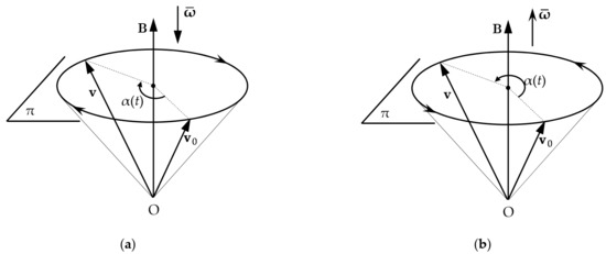
Figure 1. The hodograph of the velocity of a charged particle launched in a magnetic field with fixed direction: (a) Positive charge $q>0$; (b) Negative charge $q<0$.

The law of motion of the particle results from (68):

$$\mathbf{r}(t)={\mathbf{r}}_0+\frac{{\mathbf{v}}_0\cdot \mathbf{B}(t)}{{\mathrm{B}}^2(t)}t\mathbf{B}(t)+\frac{{\mathbf{v}}_0\times \mathbf{B}(t)}{\mathrm{B}(t)}{\displaystyle \underset{0}{\overset{t}{\int }}\sin \alpha (\mathsf{\tau })\mathrm{d}\mathsf{\tau }}+\frac{\mathbf{B}(t)\times \left({\mathbf{v}}_0\times \mathbf{B}(t)\right)}{{\mathrm{B}}^2(t)}{\displaystyle \underset{0}{\overset{t}{\int }}\cos \alpha (\mathsf{\tau })\mathrm{d}\mathsf{\tau }}.$$

(71)

This solution is pointed out in Reference [21].

2. If the electric and the magnetic fields have the same direction, $\mathbf{B}\times \mathbf{E}=0$; the solution (67) of the IVP (62) is in this case given by:

$$\mathbf{v}(t)=\frac{{\mathbf{v}}_0\cdot \mathbf{B}(t)}{{\mathrm{B}}^2(t)}\mathbf{B}(t)+\frac{{\mathbf{v}}_0\times \mathbf{B}(t)}{\mathrm{B}(t)}\sin \alpha (t)+\frac{\mathbf{B}(t)\times \left({\mathbf{v}}_0\times \mathbf{B}(t)\right)}{{\mathrm{B}}^2(t)}\cos \alpha (t)+\frac{q}{m}{\displaystyle \underset{0}{\overset{t}{\int }}\mathbf{E}(\mathsf{\tau })\mathrm{d}\mathsf{\tau }}.$$

(72)

3. If the magnetic field is uniform, $\mathbf{B}\in {\mathbf{V}}_3\Rightarrow \stackrel{.}{\mathbf{B}}=0$; the law of variation of the velocity (67) becomes:

$$\begin{array}{ll}\mathbf{v}(t)& =\frac{\left({\mathbf{v}}_0+\frac{q}{m}{\displaystyle \underset{0}{\overset{t}{\int }}\mathbf{E}(\mathsf{\tau })\mathrm{d}\mathsf{\tau }}\right)\cdot \mathbf{B}}{{\mathrm{B}}^2}\mathbf{B}+\frac{\left({\mathbf{v}}_0\sin \omega t+\frac{q}{m}{\displaystyle \underset{0}{\overset{t}{\int }}\mathbf{E}(\mathsf{\tau })\sin \omega (t-\mathsf{\tau })\mathrm{d}\mathsf{\tau }}\right)\times \mathbf{B}}{\mathrm{B}}+\\ & +\frac{\mathbf{B}\times \left[\left({\mathbf{v}}_0\cos \omega t+\frac{q}{m}{\displaystyle \underset{0}{\overset{t}{\int }}\mathbf{E}(\mathsf{\tau })\cos \omega (t-\mathsf{\tau })\mathrm{d}\mathsf{\tau }}\right)\times \mathbf{B}\right]}{{\mathrm{B}}^2},\end{array}$$

(73)

where we denoted $\omega =\frac{q\mathbf{B}}{m}$. This relation can also be written as:

$$\begin{array}{ll}\mathbf{v}(t)& =\frac{\left({\mathbf{v}}_0+\frac{q}{m}\mathbf{E}(t)\ast 1\right)\cdot \mathbf{B}}{{\mathrm{B}}^2}\mathbf{B}+\frac{\left({\mathbf{v}}_0\sin \omega t+\frac{q}{m}\mathbf{E}(t)\ast \sin \omega t\right)\times \mathbf{B}}{\mathrm{B}}+\\ & +\frac{\mathbf{B}\times \left[\left({\mathbf{v}}_0\cos \omega t+\frac{q}{m}\mathbf{E}(t)\ast \cos \omega t\right)\times \mathbf{B}\right]}{{\mathrm{B}}^2},\end{array}$$

(74)

where $\ast$ represents the convolution product (39).

3.1. Moreover, if the electric field is uniform, $\mathbf{E}\in {\mathbf{V}}_3\Rightarrow \stackrel{.}{\mathbf{E}}=0$; the law of the velocity given by (74) becomes:

$$\begin{array}{ll}\mathbf{v}(t)& =\frac{{\mathbf{v}}_0\cdot \mathbf{B}}{{\mathrm{B}}^2}\mathbf{B}+\frac{\mathbf{E}\times \mathbf{B}}{{\mathrm{B}}^2}+\frac{{\mathbf{v}}_0\times \mathbf{B}+\mathbf{E}}{\mathrm{B}}\sin \omega t+\\ & +\frac{\mathbf{B}\times ({\mathbf{v}}_0\times \mathbf{B}+\mathbf{E})}{{\mathrm{B}}^2}\cos \omega t+\frac{\mathbf{E}\cdot \mathbf{B}}{{\mathrm{B}}^3}(\omega t-\sin \omega t)\mathbf{B},\end{array}$$

(75)

solution also presented in References [21,35].

When $\mathbf{E}\cdot \mathbf{B}\ne 0$, the hodograph of the velocity is a variable pitch helix, wrapped around an elliptic cylinder whose axis of symmetry is parallel to $\mathbf{B}$. If $\mathbf{E}\cdot \mathbf{B}=0$, the hodograph becomes a circle with radius $\frac{|\mathbf{E}+{\mathbf{v}}_0\times \mathbf{B}|}{\mathrm{B}}$, located in a plane perpendicular to $\mathbf{B}$. The vector $\mathbf{v}$ sweeps the surface of a circular cone (Figure 2a); if ${\mathbf{v}}_0\cdot \mathbf{B}=0$, the vertex of the cone belongs to the plane of the circle (Figure 2b).

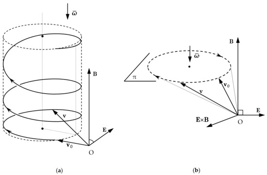
Figure 2. The hodograph of the velocity of a charged particle (q > 0) launched in uniform magnetic and electric fields: (a) The case $\mathbf{E}\cdot \mathbf{B}\ne 0$; (b) The case $\mathbf{E}\cdot \mathbf{B}=0$.

If the electric and magnetic fields are uniform, the acceleration of the charged particle $a=\stackrel{.}{\mathbf{v}}$ is obtained from (64), as the solution of the IVP:

$$\left\{\begin{array}{l}\stackrel{.}{\mathbf{a}}+\omega \times \mathbf{a}=0\\ \mathbf{a}(0)={\mathbf{a}}_0,\hspace{1em}{\mathbf{a}}_0\in {\mathbf{V}}_3,\end{array}\right.$$

(76)

where

$${\mathbf{a}}_0=\mathbf{e}-\omega \times {\mathbf{v}}_0\in {\mathbf{V}}_3.$$

(77)

It results that:

$$\mathbf{a}={\mathbf{R}}_{-\omega }{\mathbf{a}}_0={\mathbf{R}}_{-\omega }(\mathbf{e}-\omega \times {\mathbf{v}}_0).$$

(78)

It results that the force that acts at the particle has constant magnitude and performs a uniform precession around the magnetic field lines (Figure 3) with the angular velocity $\overline{\omega }=-\frac{q\mathbf{B}}{m}$.

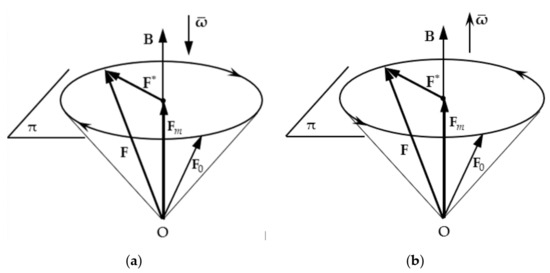
Figure 3. The force that acts at a charged particle launched in uniform electric and magnetic fields: (a) Positive charge $q>0$; (b) Negative charge $q<0$.

3.2. Suppose that the magnetic field is uniform and the intensity of the electric field has fixed direction and its variation with respect to time is $\mathbf{E}(t)=\mathbf{E}\sin ({\omega }_{0}t+\alpha )$, with $\stackrel{.}{\mathbf{E}}=0$, ${\omega }_0>0$, $\alpha \in [0,2\pi )$. In this case, (74) becomes:

$$\begin{array}{ll}\mathbf{v}(t)& =\frac{\left({\mathbf{v}}_0+\frac{q}{m}\mathbf{E}\sin ({\omega }_{0}t+\alpha )\ast 1\right)\cdot \mathbf{B}}{{\mathrm{B}}^2}\mathbf{B}+\frac{\left({\mathbf{v}}_0\sin \omega t+\frac{q}{m}\mathbf{E}\sin ({\omega }_{0}t+\alpha )\ast \sin \omega t\right)\times \mathbf{B}}{\mathrm{B}}+\\ & +\frac{\mathbf{B}\times \left[\left({\mathbf{v}}_0\cos \omega t+\frac{q}{m}\mathbf{E}\sin ({\omega }_{0}t+\alpha )\ast \cos \omega t\right)\times \mathbf{B}\right]}{{\mathrm{B}}^2}.\end{array}$$

(79)

The convolution products in (79) are:

$$\sin ({\omega }_{0}t+\alpha )\ast 1=\frac{1}{{\omega }_0}[\cos \alpha -\cos ({\omega }_{0}t+\alpha )],$$

(80)

$$\sin ({\omega }_{0}t+\alpha )\ast \sin \omega t=\left\{\begin{array}{l}\frac{\sin \left(\frac{\omega +{\omega }_0}{2}t\right)\cos \left(\frac{\omega -{\omega }_0}{2}t-\alpha \right)}{\omega +{\omega }_0}-\frac{\sin \left(\frac{\omega -{\omega }_0}{2}t\right)\cos \left(\frac{\omega +{\omega }_0}{2}t+\alpha \right)}{\omega -{\omega }_0},\mathrm{if} {\omega }_0\ne \pm \omega ,\\ -\frac{1}{2\omega }[\omega t\cos (\omega t+\alpha )-\sin \omega t\cos \alpha ],\mathrm{if} {\omega }_0=\omega ,\\ \hspace{0.33em}\hspace{0.33em}\hspace{0.17em}\frac{1}{2\omega }[\omega t\cos (\omega t-\alpha )-\sin \omega t\cos \alpha ],\mathrm{if} {\omega }_0=-\omega ,\end{array}\right.$$

(81)

and

$$\sin ({\omega }_{0}t+\alpha )\ast \cos \omega t=\left\{\begin{array}{l}-\frac{\sin \left(\frac{\omega +{\omega }_0}{2}t\right)\sin \left(\frac{\omega -{\omega }_0}{2}t-\alpha \right)}{\omega +{\omega }_0}+\frac{\sin \left(\frac{\omega -{\omega }_0}{2}t\right)\sin \left(\frac{\omega +{\omega }_0}{2}t+\alpha \right)}{\omega -{\omega }_0},\mathrm{if} {\omega }_0\ne \pm \omega ,\\ \hspace{0.33em}\hspace{0.33em}\hspace{0.17em}\frac{1}{2\omega }[\omega t\sin (\omega t+\alpha )+\sin \omega t\sin \alpha ],\mathrm{if} {\omega }_0=\omega ,\\ -\frac{1}{2\omega }[\omega t\sin (\omega t-\alpha )-\sin \omega t\sin \alpha ],\mathrm{if} {\omega }_0=-\omega ,\end{array}\right.$$

(82)

respectively. Replacing (80), (81), and (82) into (79), the velocity of the particle is obtained in each case, as follows:

$$\begin{array}{ll}\mathbf{v}(t)& =\frac{{\mathbf{v}}_0\cdot \mathbf{B}}{{\mathrm{B}}^2}\mathbf{B}+\frac{{\mathbf{v}}_0\times \mathbf{B}}{{\mathrm{B}}^2}\sin \omega t+\frac{\mathbf{B}\times ({\mathbf{v}}_0\times \mathbf{B})}{{\mathrm{B}}^2}\cos \omega t+\frac{\mathbf{E}\cdot \mathbf{B}}{{\mathrm{B}}^3}\cdot \frac{\omega }{{\omega }_0}[\cos \alpha -\cos ({\omega }_{0}t+\alpha )]+\\ & +\frac{\omega }{{\mathrm{B}}^2}\left[\frac{\sin \left(\frac{\omega +{\omega }_0}{2}t\right)\cos \left(\frac{\omega -{\omega }_0}{2}t-\alpha \right)}{\omega +{\omega }_0}-\frac{\sin \left(\frac{\omega -{\omega }_0}{2}t\right)\cos \left(\frac{\omega +{\omega }_0}{2}t+\alpha \right)}{\omega -{\omega }_0}\right]\mathbf{E}\times \mathbf{B}-\\ & -\frac{\omega }{{\mathrm{B}}^3}\left[\frac{\sin \left(\frac{\omega +{\omega }_0}{2}t\right)\sin \left(\frac{\omega -{\omega }_0}{2}t-\alpha \right)}{\omega +{\omega }_0}-\frac{\sin \left(\frac{\omega -{\omega }_0}{2}t\right)\sin \left(\frac{\omega +{\omega }_0}{2}t+\alpha \right)}{\omega -{\omega }_0}\right]\mathbf{B}\times (\mathbf{E}\times \mathbf{B}),\end{array}$$

(83)

if ${\omega }_0\ne \pm \omega$,

$$\begin{array}{ll}\mathbf{v}(t)& =\frac{{\mathbf{v}}_0\cdot \mathbf{B}}{{\mathrm{B}}^2}\mathbf{B}+\frac{{\mathbf{v}}_0\times \mathbf{B}}{{\mathrm{B}}^2}\sin \omega t+\frac{\mathbf{B}\times ({\mathbf{v}}_0\times \mathbf{B})}{{\mathrm{B}}^2}\cos \omega t+\frac{\mathbf{E}\cdot \mathbf{B}}{{\mathrm{B}}^3}[\cos \alpha -\cos ({\omega }_{0}t+\alpha )]+\\ & +\frac{\mathbf{E}\times \mathbf{B}}{2{\mathrm{B}}^2}[\omega t\cos (\omega t-\alpha )-\sin \omega t\cos \alpha ]-\frac{\mathbf{B}\times (\mathbf{E}\times \mathbf{B})}{2{\mathrm{B}}^3}\hspace{0.17em}[\omega t\sin (\omega t-\alpha )-\sin \omega t\sin \alpha ],\end{array}$$

(84)

if ${\omega }_0=\omega$, and

$$\begin{array}{ll}\mathbf{v}(t)& =\frac{{\mathbf{v}}_0\cdot \mathbf{B}}{{\mathrm{B}}^2}\mathbf{B}+\frac{{\mathbf{v}}_0\times \mathbf{B}}{{\mathrm{B}}^2}\sin \omega t+\frac{\mathbf{B}\times ({\mathbf{v}}_0\times \mathbf{B})}{{\mathrm{B}}^2}\cos \omega t+\frac{\mathbf{E}\cdot \mathbf{B}}{{\mathrm{B}}^3}[\cos \alpha -\cos ({\omega }_{0}t+\alpha )]-\\ & -\frac{\mathbf{E}\times \mathbf{B}}{2{\mathrm{B}}^2}[\omega t\cos (\omega t+\alpha )-\sin \omega t\cos \alpha ]-\frac{\mathbf{B}\times (\mathbf{E}\times \mathbf{B})}{2{\mathrm{B}}^3}\hspace{0.17em}[\omega t\sin (\omega t+\alpha )+\sin \omega t\sin \alpha ],\end{array}$$

(85)

if ${\omega }_0=-\omega$.

After finding the velocity of the particle in each of these cases, the law of motion can be easily determined by (68).

6. Exact Solution of the Rigid Body Motion in Non-Inertial Reference Frame

The pose of a rigid body with respect to a reference frame is given by an element of the special group of the displacements of the rigid body [34,37], denoted $\mathbf{S}{\mathbf{E}}_3$:

$$g=\left[\begin{array}{rr}\hfill \mathbf{Q}& \hfill \mathbf{r}\\ \hfill 0& \hfill 1\end{array}\right].$$

(86)

In (86), $\mathbf{Q}\in {\mathbf{SO}}_3$ determines the orientation (the attitude) of the rigid body with respect to the chosen reference frame, and $\mathbf{r}\in {\mathbf{V}}_3$ is the position vector of the origin of the frame attached to the rigid body. The motion of the rigid body with respect to a reference frame is given by a curve $\mathbf{g}(t)\in \mathbf{S}{\mathbf{E}}_3^{ℝ}$, where t is the variable time. This leads to the following form of the parametric equations of the motion of a rigid body:

$$\left\{\begin{array}{l}\mathbf{Q}=\mathbf{Q}(t)\in {\mathbf{SO}}_3^{ℝ}\\ \mathbf{r}=\mathbf{r}(t)\in {\mathbf{V}}_3^{ℝ}.\end{array}\right.$$

(87)

If the origin of the frame attached to the rigid body is located at the center of mass of the body, the IVP that determines the motion of the rigid body is:

$$\left\{\begin{array}{l}\ddot{\mathbf{r}}+2{\omega }_c\times \stackrel{.}{\mathbf{r}}+{\omega }_c\times ({\omega }_c\times \mathbf{r})+{\stackrel{.}{\omega }}_c\times \mathbf{r}+{\mathbf{a}}_c=\mathbf{f}\\ \mathbf{r}(t_0)={\mathbf{r}}_0\\ \stackrel{.}{\mathbf{r}}(t_0)={\mathbf{v}}_0,\hspace{1em}{\mathbf{r}}_0,{\mathbf{v}}_0\in {\mathbf{V}}_3,\hspace{1em}{\omega }_c\in {\mathbf{V}}_3^{{ℝ}_{+}},\end{array}\right.$$

(88)

$$\left\{\begin{array}{l}\stackrel{.}{\mathbf{Q}}=\tilde{\omega }\mathbf{Q}\\ \stackrel{.}{\omega }+{\stackrel{.}{\omega }}_c=\mathbf{Q}{J}^{-1}[\mathsf{\tau }-{\mathbf{Q}}^T(\omega +{\omega }_c)\times J{\mathbf{Q}}^T(\omega +{\omega }_c)]+\omega \times {\omega }_c\\ \omega (t_0)={\omega }_0,\hspace{1em}{\omega }_0\in {\mathbf{V}}_3\\ \mathbf{Q}(t_0)={\mathbf{Q}}_0,\hspace{1em}{\mathbf{Q}}_0\in \mathrm{s}{\mathbf{O}}_3.\end{array}\right.$$

(89)

In (88) $\mathbf{r}\in {\mathbf{V}}_3^{ℝ}$ is the position vector of the center of mass of the rigid body with respect to the non-inertial reference frame (NIRF), ${\omega }_c$ is the instantaneous angular velocity of the NIRF, ${\mathbf{a}}_c$ is the acceleration of the origin of the NIRF, and $\mathbf{F}=\frac{\mathcal{R}}{m}$, where $\mathcal{R}$ is the resultant of the forces which act at the center of mass. The vectors ${\mathbf{R}}_0\in {\mathbf{V}}_3$ and ${\mathbf{V}}_0\in {\mathbf{V}}_3$ represent the initial position and the initial velocity of the center of mass with respect to the NIFR, respectively.

In (89), the tensor $\mathbf{Q}\in \mathbf{S}{\mathbf{O}}_3^{ℝ}$ gives the attitude of the rigid body in relation with the NIRF, ω is the instantaneous angular velocity of the rigid body in relation with the NIRF, τ is the resulting torque of the forces applied on the rigid body in relation with its mass center, J is the inertia tensor of the rigid body in relation with its mass center, ${\omega }_0$ is the angular velocity of the rigid body with respect to the NIRF at the moment $t_0$, and ${\mathbf{Q}}_0$ is the orientation of the rigid body with respect to the NIRF at the moment $t_0$.

Let ${\mathbf{R}}_{-{\omega }_c}$ be the unique solution of the IVP:

$$\left\{\begin{array}{l}\stackrel{.}{\mathbf{R}}+{\tilde{\omega }}_c\mathbf{R}=0\\ \mathbf{R}(t_0)=I_3.\end{array}\right.$$

(90)

Theorem 11. 

The solution to the IVP (88) is obtained by applying the tensor ${\mathbf{R}}_{-{\omega }_c}^{}$ to the problem:

$$\left\{\begin{array}{l}\ddot{\mathbf{r}}={\mathbf{R}}_{-{\omega }_c}^T(\mathbf{f}-{\mathbf{a}}_c)\\ \mathbf{r}(t_0)={\mathbf{r}}_0\\ \stackrel{.}{\mathbf{r}}(t_0)={\mathbf{v}}_0+{\omega }_c(t_0)\times {\mathbf{r}}_0.\end{array}\right.$$

(91)

Proof. 

Taking into account the differentiation rule (14), the differential equation in the IVP (88) can be written as:

$${\mathbf{r}}^{″}=\mathbf{f}-{\mathbf{a}}_c.$$

(92)

Applying ${\mathbf{F}}_{\omega }$ to Equation (92), we obtain ${\mathbf{F}}_{{\omega }_c}{\mathbf{r}}^{″}={\mathbf{F}}_{{\omega }_c}(\mathbf{f}-{\mathbf{a}}_c)$, or, from point (8.) of Lemma 3:

$$\frac{{\mathrm{d}}^2}{\mathrm{d}{t}^2}({\mathbf{F}}_{{\omega }_c}\mathbf{r})={\mathbf{F}}_{{\omega }_c}(\mathbf{f}-{\mathbf{a}}_c).$$

(93)

The conclusion of the theorem is proved if we now replace r with $\mathbf{r}\to {\mathbf{F}}_{\omega }\mathbf{r}$. □

In what follows, we give a representation theorem for the tensor $\mathbf{Q}\in {\mathbf{SO}}_3^{ℝ}$, which parameterizes the rotation of the rigid body around its center of mass; this motion is recovered from the IVP (89).

Theorem 12. 

The solution to the IVP (89) results by applying${\mathbf{R}}_{-{\omega }_c}$ to the solution of the Euler fixed point classic problem:

$$\left\{\begin{array}{l}{\stackrel{.}{\mathbf{Q}}}_{\ast }={\mathbf{Q}}_{\ast }{\tilde{\omega }}_{\ast }\\ J{\stackrel{.}{\omega }}_{\ast }+{\omega }_{\ast }\times J{\omega }_{\ast }={\tau }_{\ast }\\ {\omega }_{\ast }(t_0)={\mathbf{Q}}_0^T({\omega }_0+{\omega }_c(t_0))\\ {\mathbf{Q}}_{\ast }(t_0)={\mathbf{Q}}_0.\end{array}\right.$$

(94)

Proof. 

In (89), consider the following change of variable:

$${\omega }_{\ast }={\mathbf{Q}}^T(\omega +{\omega }_c).$$

(95)

It leads to ${\stackrel{.}{\omega }}_{\ast }={\stackrel{.}{\mathbf{Q}}}^T(\omega +{\omega }_c)+{\mathbf{Q}}^T(\stackrel{.}{\omega }+{\stackrel{.}{\omega }}_c)=-{\mathbf{Q}}^T\tilde{\omega }(\omega +{\omega }_c)+{\mathbf{Q}}^T(\stackrel{.}{\omega }+{\stackrel{.}{\omega }}_c)$, which is equivalent with ${\stackrel{.}{\omega }}_{\ast }={\stackrel{.}{\mathbf{Q}}}^T({\omega }_c\times \omega +\stackrel{.}{\omega }+{\stackrel{.}{\omega }}_c)$, or

$${\omega }_c\times \omega +\stackrel{.}{\omega }+{\stackrel{.}{\omega }}_c=\mathbf{Q}{\stackrel{.}{\omega }}_{\ast }.$$

(96)

After some calculation, from (95), (96), and (89), it results that

$$\left\{\begin{array}{l}J{\stackrel{.}{\omega }}_{\ast }+{\omega }_{\ast }\times J{\omega }_{\ast }={\tau }_{\ast }\\ {\omega }_{\ast }(t_0)={\mathbf{Q}}_0^T({\omega }_0+{\omega }_c(t_0)),\end{array}\right.$$

(97)

where ${\tau }_{\ast }={\mathbf{Q}}^T\tau$ is the in-body torque related to the center of mass in the body frame of the rigid body.

The problem (97) is a Euler fixed point classic problem. For any $\mathbf{Q}\in \mathbf{S}{\mathbf{O}}_3^{ℝ}$, the solution of (97) is obtained from:

$$\left\{\begin{array}{l}\stackrel{.}{\mathbf{Q}}=\tilde{\omega }\mathbf{Q}\\ \mathbf{Q}(t_0)={\mathbf{Q}}_0.\end{array}\right.$$

(98)

From (95), it results that $\mathbf{Q}{\omega }_{\ast }=\omega +{\omega }_c$. Applying the operator ∼, this relation becomes ${\widetilde{\mathbf{Q}\omega }}_{\ast }=\tilde{\omega }+{\tilde{\omega }}_c\iff \mathbf{Q}{\tilde{\omega }}_{\ast }{\mathbf{Q}}^T=\stackrel{.}{\mathbf{Q}}{\mathbf{Q}}^T+{\tilde{\omega }}_c$. After right multiplying the last expression by Q, we obtain the IVP:

$$\left\{\begin{array}{l}\stackrel{.}{\mathbf{Q}}=\mathbf{Q}{\tilde{\omega }}_{\ast }-{\tilde{\omega }}_c\mathbf{Q}\\ \mathbf{Q}(t_0)={\mathbf{Q}}_0.\end{array}\right.$$

(99)

Considering now $\mathbf{Q}={\mathbf{R}}_{-{\omega }_c}{\mathbf{Q}}_{\ast }$, the theorem is proved. □

7. Conclusions

The paper presents a new general method for studying motion in a non-inertial reference frame, using the properties of the Lie groups ${\mathbf{SO}}_3$ and $\mathbf{S}{\mathbf{E}}_3$. This method is based on proper orthogonal and skew-symmetric tensor valued functions, introduced by the Poisson-Darboux equation and an appropriately defined differentiation operator, as a function of the instantaneous angular velocity of the non-inertial reference frame. Three applications are presented: the motion in a gravitational force field with respect to a rotating reference frame, the motion of a charged particle in non-stationary electric and magnetic fields, and the exact solution of the rigid body motion in the non-inertial reference frame. The results are closed-form and coordinate-free.

References

- Levi Civita, T.; Amaldi, U. Lezioni di Mecanica Razionale; Nicola Zanichelli: Bologna, Italy, 1926. [Google Scholar]
- Arnold, V. Les Méthodes Mathématiques de la Mécanique Classique; Éd. Mir: Moscow, Russia, 1976. [Google Scholar]
- Arya, A.P. Introduction to Classical Mechanics, 2nd ed.; Prentice Hall International: Hoboken, NJ, USA, 1998. [Google Scholar]
- French, A.P. Newtonian Mechanics; Norton: New York, NY, USA, 1971. [Google Scholar]
- Feynman, R.P.; Leighton, R.B.; Sands, M. The Feynman Lectures on Physics, Vol. 1: Mainly Mechanics, Radiation, and Heat; Addison-Wesley: Reading, UK, 1963. [Google Scholar]
- Barger, V.; Olsson, M. Classical Mechanics: A Modern Perspective, 2nd ed.; McGraw Hill: New York, NY, USA, 1995. [Google Scholar]
- Corben, H.C.; Stehle, P. Classical Mechanics, 2nd ed.; Dover: New York, NY, USA, 1994. [Google Scholar]
- Fetter, L.A.; Walecka, J.D. Theoretical Mechanics of Particles and Continua; Dover: New York, NY, USA, 2013. [Google Scholar]
- Fowles, G.R.; Cassiday, G.L. Analytical Dynamics, 7th ed.; Thompson Brooks/Cole: Belmont, Japan, 2005. [Google Scholar]
- Hand, L.N.; Finch, J.D. Analytical Mechanics; Cambridge University Press: Cambridge, UK, 1998. [Google Scholar]
- Hestenes, D. New Foundations for Classical Mechanics, 2nd ed.; Springer: Dordrecht, The Netherlands, 1999. [Google Scholar] [CrossRef]
- José, J.V.; Saletan, E.J. Classical Dynamics. A Contemporary Approach; Cambridge University Press: Cambridge, UK, 1998. [Google Scholar] [CrossRef]
- Thornton, S.T.; Marion, J.B. Classical Dynamics of Particles and Systems, 5th ed.; Brooks/Cole—Thompson Learning: Belmont, Japan, 2004. [Google Scholar]
- Teodorescu, P.P. Mechanical Systems, Classical Models, Volume I: Particle Mechanics; Springer: Dordrecht, The Netherlands, 2007. [Google Scholar] [CrossRef]
- Teodorescu, P.P. Mechanical Systems, Classical Models, Volume II: Mechanics of Discrete and Continuous Systems; Springer: Dordrecht, The Netherlands, 2009. [Google Scholar] [CrossRef]
- Deriglazov, A. Classical Mechanics. Hamiltonian and Lagrangian Formalism, 2nd ed.; Springer International: Berlin/Heidelberg, Germany, 2017. [Google Scholar] [CrossRef]
- Strauch, D. Classical Mechanics. An Introduction; Springer: Berlin/Heidelberg, Germany, 2009. [Google Scholar] [CrossRef]
- Benacquista, M.J.; Romano, J.D. Classical Mechanics; Springer International: Berlin/Heidelberg, Germany, 2018. [Google Scholar] [CrossRef]
- Awrejcewicz, J. Classical Mechanics. Kinematics and Statics; Springer: New York, NY, USA, 2012. [Google Scholar] [CrossRef]
- Ilisie, V. Lectures in Classical Mechanics. With Solved Problems and Exercises; Springer International: Berlin/Heidelberg, Germany, 2020. [Google Scholar] [CrossRef]
- Condurache, D. New Symbolic Procedures in the Study of Dynamical Systems. Ph.D. Thesis, Gheorghe Asachi Technical University of Iasi, Iasi, Romania, 1995. [Google Scholar]
- Condurache, D.; Martinuși, V. Kepler’s Problem in Rotating Reference Frames. Part I: Prime Integrals. Vectorial Regularization. J. Guid. Control Dyn. 2007, 30, 192–200. [Google Scholar] [CrossRef]
- Condurache, D.; Martinuși, V. Kepler’s Problem in Rotating Reference Frames. Part II: Relative Orbital Motion. J. Guid. Control Dyn. 2007, 30, 201–213. [Google Scholar] [CrossRef]
- Condurache, D.; Martinuși, V. Foucault Pendulum-like problems: A tensorial approach. Int. J. Non Linear Mech. 2008, 43, 743–760. [Google Scholar] [CrossRef][Green Version]
- Condurache, D.; Martinuși, V. Exact Solution to the Relative Orbital Motion in Eccentric Orbits. Sol. Syst. Res. 2009, 43, 41–52. [Google Scholar] [CrossRef]
- Condurache, D.; Martinuși, V. Relative Spacecraft Motion in a Central Force Field. J. Guid. Control Dyn. 2007, 30, 873–876. [Google Scholar] [CrossRef]
- Condurache, D.; Martinuși, V. Exact Solution to the Relative Orbital Motion in a Central Force Field. In Proceedings of the 2nd IEEE/AIAA International Symposium on Systems and Control in Aerospace and Astronautics, Shenzhen, China, 10–12 December 2008. [Google Scholar] [CrossRef]
- Condurache, D.; Martinuși, V. A Quaternionic Exact Solution to the Relative Orbital Motion Problem. J. Guid. Control Dyn. 2010, 30, 201–213. [Google Scholar] [CrossRef]
- Darboux, G. Leçons sur la Théorie Générale des Surfaces et les Applications Géométriques du Calcul Infinitésimal, Volume 1; Gauthier-Villars: Paris, France, 1887. [Google Scholar]
- Condurache, D. Poisson-Darboux Problem’s Extended in Dual Lie Algebra. Adv. Astronaut. Sci. 2018, 162, 3345–3364. [Google Scholar]
- Zhilin, P.A. A New Approach to the Analysis of Free Rotation of Rigid Bodies. ZAMM 1996, 76, 187–204. [Google Scholar] [CrossRef]
- Itskov, M. Tensor Algebra and Tensor Analysis for Engineering with Applications to Continuum Mechanics; Springer: New York, NY, USA, 2009. [Google Scholar] [CrossRef]
- Fasano, A.; Marmi, S. Analytical Mechanics: An Introduction; Oxford University Press: Oxford, UK, 2013. [Google Scholar]
- Angeles, J. Fundamentals of Robotic Mechanical Systems. Theory, Methods, and Algorithms, 4th ed.; Springer: New York, NY, USA, 2014. [Google Scholar] [CrossRef]
- Landau, L.; Lifchitz, E. Mécanique; Éd. Mir: Moscow, Russia, 1981. [Google Scholar]
- Arnold, V.I.; Kozlov, V.; Neishtadt, A. Mathematical Aspects of Classical and Celestial Mechanics, 3rd ed.; Springer: New York, NY, USA, 2006. [Google Scholar] [CrossRef]
- Marsden, J.E.; Ratiu, T.S. Introduction to Mechanics and Symmetry, 2nd ed.; Springer: New York, NY, USA, 1999. [Google Scholar] [CrossRef]
- Goldstein, H.; Safko, J.L.; Poole, C.P. Classical Mechanics, 3rd ed.; Pearson: Harlow, UK, 2002. [Google Scholar]
- Martinuși, V. Lagrangian and Hamiltonian Formulations in Relative Orbital Dynamics. Applications to Spacecraft Formation Flying and Satellite Constellations. Ph.D. Thesis, Technical University Gheorghe Asachi, Iasi, Romania, 2010. [Google Scholar]
- Gantmacher, F.R. The Theory of Matrices; Chelsea Pub. Co.: New York, NY, USA, 1959. [Google Scholar]
- Artsimovitch, L.A.; Loukianov, S. Mouvements des Particules Chargées Dans des Champs Électriques et Magnétiques; Éditions Mir: Moscow, Russia, 1975. [Google Scholar]
- Krall, N.A.; Trivelpiece, A.W. Principles of Plasma Physics; McGraw-Hill: New York, NY, USA, 1973. [Google Scholar]
Publisher’s Note: MDPI stays neutral with regard to jurisdictional claims in published maps and institutional affiliations. |
© 2021 by the authors. Licensee MDPI, Basel, Switzerland. This article is an open access article distributed under the terms and conditions of the Creative Commons Attribution (CC BY) license (https://creativecommons.org/licenses/by/4.0/).