Exponentiated Generalized Inverted Gompertz Distribution: Properties and Estimation Methods with Applications to Symmetric and Asymmetric Data

Abstract

In this article, a new four-parameter lifetime model called the exponentiated generalized inverted Gompertz distribution is studied and proposed. The newly proposed distribution is able to model the lifetimes with upside-down bathtub-shaped hazard rates and is suitable for describing the negative and positive skewness. A detailed description of some various properties of this model, including the reliability function, hazard rate function, quantile function, and median, mode, moments, moment generating function, entropies, kurtosis, and skewness, mean waiting lifetime, and others are presented. The parameters of the studied model are appreciated using four various estimation methods, the maximum likelihood, least squares, weighted least squares, and Cramér-von Mises methods. A simulation study is carried out to examine the performance of the new model estimators based on the four estimation methods using the mean squared errors (MSEs) and the bias estimates. The flexibility of the proposed model is clarified by studying four different engineering applications to symmetric and asymmetric data, and it is found that this model is more flexible and works quite well for modeling these data.

1. Introduction

In reliability analysis and life testing situations, we can define the times of occurrence of events under study as the “survival times” or “failure times” or “lifetimes”. The events under study may be the death of an individual, health code compliance, development of disease symptoms, and failure of a device. In almost all applied sciences and fields, such as life testing problems, medical and biological sciences, environmental studies, economics, engineering, insurance and finance, amongst others, statisticians and researchers are interested in the analysis and modeling of real lifetime data using the statistical distributions. Due to the importance and usefulness of statistical distributions in predicting and describing the real-world phenomena in these fields, there has been great attention in developing and finding more flexible models over the last decades [1]. Extending the exponential distribution by introducing the Gompertz (G) distribution. It is a very popular and widely used lifetime model due to its wide applicability in a lot of fields, such as biology, demography, computer and marketing sciences, actuaries, and gerontology. Furthermore, it has been widely used in survival analysis describing human deaths, growth models, and preparing the actuarial tables. An influential characteristic of the G distribution, which decreases its usefulness and flexibility, is that it only has an increasing failure rate. Therefore, some extensions or modifications of the G distribution are proposed and studied in the statistical literature to provide more flexibility in lifetime modeling; for example, see [2,3,4,5,6,7,8]. Ref [9] studied and proposed a two-parameter lifetime probability distribution, which is called the inverted Gompertz (IG) distribution, with a hazard rate function, which is an upside-down bathtub-shaped curve. The cumulative distribution function (CDF) and the probability density function (PDF) of the random variable $Y$ that has the IG with the two parameters $\alpha >0$ and $\beta >0$ are given, respectively, as

$$G\left(y\right)=e^{-\frac{\alpha }{\beta }\left({\mathrm{e}}^{\frac{\beta }{y}}-1\right)}; y>0; \alpha , \beta >0$$

(1)

and

$$g\left(y\right)=\frac{\alpha }{y^2}{e}^{\frac{\beta }{y}} e^{-\frac{\alpha }{\beta }\left(e^{\frac{\beta }{y}}-1\right)}; y>0; \alpha , \beta >0.$$

(2)

If we put $\alpha =1$ in Equations (1) and (2), we will get the CDF and PDF of the Adaptable (A) distribution studied by [10]. In the last few years, many various generalizations have received increased interest in the literature, for example [11,12,13,14,15,16,17,18,19,20,21,22,23]. Ref [17] introduced a new class of univariate distributions, which is considered as a generalization of the exponentiated type distributions, and mentioned its structural and statistical properties. They defined the exponentiated generalized (EG) class of distributions whose CDF and PDF are obtained, respectively, by

$$F\left(x\right)={\left[1-{\left(1-G\left(x\right)\right)}^{\gamma }\right]}^{\theta }$$

(3)

and

$$f\left(x\right)=\gamma \theta g\left(x\right){\left(1-G\left(x\right)\right)}^{\gamma -1}{\left[1-{\left(1-G\left(x\right)\right)}^{\gamma }\right]}^{\theta -1},$$

(4)

where $G\left(x\right)$ and $g\left(x\right)$ represent the CDF and PDF of the baseline random variable. Further, $\gamma >0$ and $\theta >0$ are two supplementary shape parameters that make the skewness more flexible if it is compared with the baseline model. In this paper, the so-called exponentiated generalized inverted Gompertz distribution, abbreviated to EGIG, with four parameters, is proposed by substituting from Equations (1) and (2) into Equations (3) and (4). This model is capable of modeling the failure rates characterized by an upside-down bathtub-shaped curve and is appropriate for describing the positive and negative skewness. Moreover, the EGIG model has some lifetime sub-models, such as the IG, A, and exponentiated generalized A (EGA) distribution, which extends the A distribution. Finally, the suggested model is suitable to prescribe symmetric and asymmetric data numerically.

Our paper is classified as follows: Section 2 introduces the EGIG distribution. In Section 3, some essential and fundamental statistical characteristics of the EGIG are presented. Four various estimation methods are studied to determine the EGIG parameters in Section 4. The goodness of the EGIG estimators is assessed by a simulation study in Section 5. Four real data sets from engineering are analyzed, and the results are compared to some well-known distributions in Section 6. Finally, a brief conclusion is presented for the results in Section 7.

2. Exponentiated Generalized Inverted Gompertz Distribution

Assume $X$ to be a non-negative random variable that has the $\mathrm{EGIG}$ with the parameters vector $\Omega =\left(\alpha , \beta , \gamma , \theta \right)$, say $X\sim \mathrm{EGIG}\left(\Omega \right)$, if the CDF of $X$ is given by

$$F\left(x\right)={\left[1-{\left(1-e^{-\frac{\alpha }{\beta }\left(e^{\frac{\beta }{x}}-1\right)}\right)}^{\gamma }\right]}^{\theta }; x>0; \alpha , \beta , \gamma , \theta >0.$$

(5)

The PDF of the EGIG is found by

$$f\left(x\right)=\frac{\alpha \gamma \theta }{x^2}{e}^{\frac{\beta }{x}}{e}^{-\frac{\alpha }{\beta }\left(e^{\frac{\beta }{x}}-1\right)}{\left(1-e^{-\frac{\alpha }{\beta }\left(e^{\frac{\beta }{x}}-1\right)}\right)}^{\gamma -1}{\left[1-{\left(1-e^{-\frac{\alpha }{\beta }\left(e^{\frac{\beta }{x}}-1\right)}\right)}^{\gamma }\right]}^{\theta -1}; x>0; \alpha , \beta , \gamma , \theta >0$$

(6)

where the parameter $\beta$ is the scale parameter and the three parameters $\alpha , \gamma$, and $\theta$ are the shape parameters that make the EGIG more useful and flexible. Setting $\gamma =\theta =1$ in Equations (5) and (6), we will obtain the CDF and PDF of the IG model. Furthermore, if we put $\alpha =\gamma =\theta =1$ in these equations, we will get the CDF and PDF of the A model. Finally, if we substitute $\alpha =1$ into Equations (5) and (6), we will obtain the CDF and PDF of a new distribution, which can be named “exponentiated generalized A (EGA) distribution”. This confirms the fact that the new model extends the IG, A, and EGA distributions. The reliability function of $X$ is obtained by

$$R\left(x\right)=1-{\left[1-{\left(1-e^{-\frac{\alpha }{\beta }\left(e^{\frac{\beta }{x}}-1\right)}\right)}^{\gamma }\right]}^{\theta }.$$

(7)

The failure rate function (HRF) of $X$ and its reversed HRF are expressed by

$$h\left(x\right)=\frac{\frac{\alpha \gamma \theta }{x^2}{e}^{\frac{\beta }{x}}{e}^{-\frac{\alpha }{\beta }\left(e^{\frac{\beta }{x}}-1\right)}{\left(1-e^{-\frac{\alpha }{\beta }\left(e^{\frac{\beta }{x}}-1\right)}\right)}^{\gamma -1}{\left[1-{\left(1-e^{-\frac{\alpha }{\beta }\left(e^{\frac{\beta }{x}}-1\right)}\right)}^{\gamma }\right]}^{\theta -1}}{1-{\left[1-{\left(1-e^{-\frac{\alpha }{\beta }\left(e^{\frac{\beta }{x}}-1\right)}\right)}^{\gamma }\right]}^{\theta }}$$

(8)

and

$$r\left(x\right)=\frac{\frac{\alpha \gamma \theta }{x^2}{e}^{\frac{\beta }{x}}{e}^{-\frac{\alpha }{\beta }\left(e^{\frac{\beta }{x}}-1\right)}{\left(1-e^{-\frac{\alpha }{\beta }\left(e^{\frac{\beta }{x}}-1\right)}\right)}^{\gamma -1}}{1-{\left(1-e^{-\frac{\alpha }{\beta }\left(e^{\frac{\beta }{x}}-1\right)}\right)}^{\gamma }}.$$

(9)

Figure 1 represents the graphical performance of the HRF and PDF for EGIG with various choices of $\alpha$, $\beta$, $\gamma ,$ and $\theta$. It is obvious that the HRF has an upside-down bathtub-shaped curve, and the PDF is unimodal-shaped.

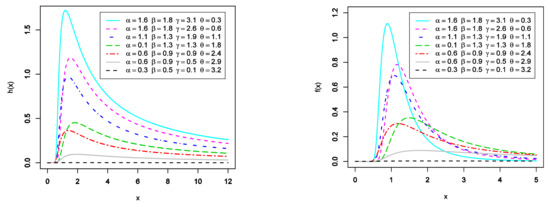
Figure 1. The plots of HRF (left panel) and PDF (right panel) for EGIG with different choices of $\alpha$, $\beta$, $\gamma$, and $\theta$.

3. Statistical and Mathematical Properties of EGIG

3.1. The Quantile Function and Median

We will derive, in this subsection, the quantile function and median for the new model. Assume $X\sim \mathrm{EGIG}\left(\Omega \right)$, then the quantile $x_q$ of the EGIG is given as follows

$$x_q=\frac{\beta }{\ln \left\{1-\frac{\beta }{\alpha } ln\left(1-{\left(1-q^{\frac{1}{\theta }}\right)}^{\frac{1}{\gamma }}\right)\right\}};0<q<1 .$$

(10)

Setting $q=\frac{1}{2}$ in Equation (10) to get the median of the EGIG as follows

$$Med\left(X\right)=\frac{\beta }{\ln \left\{1-\frac{\beta }{\alpha } ln\left(1-{\left(1-{\left(\frac{1}{2}\right)}^{\frac{1}{\theta }}\right)}^{\frac{1}{\gamma }}\right)\right\}}$$

(11)

3.2. The Mode

Assume $X\sim \mathrm{EGIG}\left(\Omega \right)$, then we can solve the following non-linear equation for $x$ to find the mode of $X$.

$$\alpha e^{\frac{\beta }{x}}\left\{\frac{\gamma \left(\theta -1\right)}{e^{\frac{\alpha }{\beta }\left(e^{\frac{\beta }{x}}-1\right)}\left[{\left(1-e^{-\frac{\alpha }{\beta }\left(e^{\frac{\beta }{x}}-1\right)}\right)}^{1-\gamma }-1\right]+1}+\left(1-\frac{\gamma -1}{e^{\frac{\alpha }{\beta }\left(e^{\frac{\beta }{x}}-1\right)}-1}\right)\right\}-2x-\beta =0.$$

(12)

We can use some numerical methods to conclude the solution of the above equation.

3.3. The $r\mathrm{th}$ Moment

The $r\mathrm{th}$ moment of $X\sim \mathrm{EGIG}\left(\Omega \right)$ is found by

$${\mu }^{\left(r\right)}=E\left(x^r\right)=\underset{0}{\overset{\infty }{{\displaystyle \int }}}{x}^{r}f\left(x\right)dx.$$

(13)

Substitute from Equation (6) into Equation (13), and we will obtain the $r\mathrm{th}$ moment as follows

$$\begin{array}{cc}{\mu }^{\left(r\right)}& ={\displaystyle {\displaystyle \sum }_{\ell =0}^{\theta -1}{\displaystyle \sum }_{k=0}^{\gamma \left(\ell +1\right)-1}{\displaystyle \sum }_{i=0}^{\infty }{\displaystyle \sum }_{j=0}^i{\displaystyle \sum }_{m=0}^{\infty }}\left(\begin{array}{c}\theta -1\\ \ell \end{array}\right)\left(\begin{array}{c}\gamma \left(\ell +1\right)-1\\ k\end{array}\right)\hfill \\ & \times \frac{{\left(-1\right)}^{i+j+k+\ell +1}{\left(k+1\right)}^i{\left(1+i\right)}^m{\alpha }^{i+1}{\beta }^{r-i-1}{j}^{r-m-1}\gamma \theta \mathsf{\Gamma }\left(m-r+1\right)}{j!m!\left(i-j\right)!}.\hfill \end{array}$$

(14)

3.4. The Moment Generating Function

Assume $X\sim \mathrm{EGIG}\left(\Omega \right)$, then the moment generating function of the EGIG can be obtained as

$$M_X\left(t\right)=E\left(e^{tx}\right)={\displaystyle \sum }_{r=0}^{\infty }\frac{t^r}{r!}{{\displaystyle \int }}_0^{\infty }{x}^{r}f\left(x;\Omega \right)dx={\displaystyle \sum }_{r=0}^{\infty }\frac{t^r}{r!}{\mu }^{\left(r\right)}$$

(15)

Substitute from Equation (14) into Equation (15), we conclude that

$$\begin{array}{cc}{M}_X\left(t\right)& ={\displaystyle {\displaystyle \sum }_{r=0}^{\infty }{\displaystyle \sum }_{\ell =0}^{\theta -1}{\displaystyle \sum }_{k=0}^{\gamma \left(\ell +1\right)-1}{\displaystyle \sum }_{i=0}^{\infty }{\displaystyle \sum }_{j=0}^i{\displaystyle \sum }_{m=0}^{\infty }}\left(\begin{array}{c}\theta -1\\ l\end{array}\right)\left(\begin{array}{c}\gamma \left(\ell +1\right)-1\\ k\end{array}\right)\hfill \\ & \times \frac{{\left(-1\right)}^{i+j+k+\ell +1}{\left(k+1\right)}^i{\left(1+i\right)}^m{\alpha }^{i+1}{\beta }^{r-i-1}{j}^{r-m-1}\gamma \theta t^r\mathsf{\Gamma }\left(m-r+1\right)}{r!j!m!\left(i-j\right)!}.\hfill \end{array}$$

(16)

3.5. Probability-Weighted Moment

The expectation of a specific function of $X$, which is used to appreciate the parameters of a certain distribution that has no explicit formula for its inverse form is called the probability-weighted moment (PWM). The PWM of $X$ whose CDF $F\left(x\right)$, say ${\xi }_{s,r}$, is determined by

$${\xi }_{s,r}=E\left(x^s{F}^r\left(x\right)\right)=\underset{0}{\overset{\infty }{{\displaystyle \int }}}{x}^s{F}^r\left(x\right)f\left(x\right)dx.$$

(17)

If $X\sim \mathrm{EGIG}\left(\Omega \right)$, then the PWM ${\xi }_{s,r}$ is found by

$$\begin{array}{cc}{\xi }_{s,r}& ={\displaystyle {\displaystyle \sum }_{\ell =0}^{\theta \left(r+1\right)-1}{\displaystyle \sum }_{k=0}^{\gamma \left(\ell +1\right)-1}{\displaystyle \sum }_{i=0}^{\infty }{\displaystyle \sum }_{j=0}^i{\displaystyle \sum }_{m=0}^{\infty }}\left(\begin{array}{c}\theta \left(r+1\right)-1\\ l\end{array}\right)\left(\begin{array}{c}\gamma \left(\ell +1\right)-1\\ k\end{array}\right)\hfill \\ & \times \frac{{\left(-1\right)}^{i+j+k+\ell +1}{\left(k+1\right)}^i{\left(1+i\right)}^m{\alpha }^{i+1}{\beta }^{s-i-1}{j}^{s-m-1}\gamma \theta \mathsf{\Gamma }\left(m-s+1\right)}{j!m!\left(i-j\right)!}\hfill \end{array}$$

(18)

3.6. Entropy Function and $\rho$ -Entropy

The entropy function is a measure of variability for the uncertainty related to $X$ whose PDF $f\left(x\right)$. It plays a fundamental role in computer science, engineering, and others. The Rényi entropy of $X$, say $I_{\rho }\left(X\right)$, is determined using

$$I_{\rho }\left(X\right)=\frac{1}{1-\rho }log\underset{0}{\overset{\infty }{{\displaystyle \int }}}{f}^{\rho }\left(x\right)dx, \rho \in \left]0, \infty \right[-\left\{1\right\}.$$

(19)

If $X\sim \mathrm{EGIG}\left(\Omega \right)$, then $I_{\rho }\left(X\right)$ is obtained by

$$\begin{array}{cc}{I}_{\rho }\left(X\right)& =\frac{1}{1-\rho }log\left\{{\displaystyle {\displaystyle \sum }_{\ell =0}^{\rho \left(\theta -1\right)}{\displaystyle \sum }_{k=0}^{\gamma \left(\ell +\rho \right)-\rho }{\displaystyle \sum }_{i=0}^{\infty }{\displaystyle \sum }_{j=0}^i{\displaystyle \sum }_{m=0}^{\infty }}\left(\begin{array}{c}\rho \left(\theta -1\right)\\ l\end{array}\right)\left(\begin{array}{c}\gamma \left(\ell +\rho \right)-\rho \\ k\end{array}\right)\right.\hfill \\ & \times \left.\frac{{\left(-1\right)}^{i+j+k+\ell +1}{\left(\rho +k\right)}^i{\left(\rho +i\right)}^m{\alpha }^{\rho +i}{\beta }^{-2\rho -i+1}{j}^{-2\rho -m+1}{\gamma }^{\rho }{\theta }^{\rho } \mathsf{\Gamma }\left(2\rho +m-1\right)}{j!m!\left(i-j\right)!}\right\}\hfill \end{array}$$

(20)

Further, the $\rho -$entropy of $X$, say $H_{\rho }\left(X\right)$, takes the formula

$$H_{\rho }\left(X\right)=\frac{1}{1-\rho }log\left[1-\left(1-\rho \right)I_{\rho }\left(X\right)\right]$$

(21)

3.7. Skewness and Kurtosis

We can use the quantiles of the EGIG distribution given in Equation (10) to examine the effect of $\gamma$ and $\theta$ (shape parameters) on the skewness ($S_k$) and the kurtosis ($K_u$). The Bowley skewness proposed by [24] is determined by

$$S_k=\frac{q\left(0.75\right)+q\left(0.25\right)-2q\left(0.5\right)}{q\left(0.75\right)-q\left(0.25\right)}.$$

(22)

Furthermore, the Moors kurtosis proposed by [25] is determined by

$$K_u=\frac{q\left(0.375\right)+q\left(0.875\right)-q\left(0.625\right)-q\left(0.125\right)}{q\left(0.75\right)-q\left(0.25\right)},$$

(23)

where $q\left(.\right)$ represents the quantiles of $X$. Figure 2 illustrates the plots of $K_u$ and $S_k$ for various choices of $\gamma$ as $\alpha =1.5$ and $\beta =0.5$. It shows that the EGIG is suitable for modeling the negative and positive skewness, and also both $S_k$ and $K_u$ are sensitive to the shape parameters $\gamma$ and $\theta$.

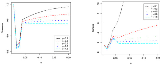
Figure 2. The plots of $S_k$ (left panel) and the plots of $K_u$ (right panel) for the EGIG model.

3.8. Mean Time to Failure

Assume $X\sim \mathrm{EGIG}\left(\Omega \right)$, then the mean time to failure of $X$, say $MTTF$, is given using

$$MTTF={{\displaystyle \int }}_0^{\infty }xf\left(x;\Omega \right)dx={\mu }^{\left(1\right)}.$$

Substitute from Equation (14), as $=1$, to obtain

$$\begin{array}{cc}MTTF& ={\displaystyle {\displaystyle \sum }_{\ell =0}^{\theta -1}{\displaystyle \sum }_{k=0}^{\gamma \left(\ell +1\right)-1}{\displaystyle \sum }_{i=0}^{\infty }{\displaystyle \sum }_{j=0}^i{\displaystyle \sum }_{m=0}^{\infty }}\left(\begin{array}{c}\theta -1\\ l\end{array}\right)\left(\begin{array}{c}\gamma \left(\ell +1\right)-1\\ k\end{array}\right)\hfill \\ & \times \frac{{\left(-1\right)}^{i+j+k+\ell +1}{\left(k+1\right)}^i{\left(1+i\right)}^m{\alpha }^{i+1}{\beta }^{-i}{j}^{-m}\gamma \theta \mathsf{\Gamma }\left(m\right)}{j!m!\left(i-j\right)!}\hfill \end{array}$$

(24)

3.9. Mean Residual and Waiting Lifetimes

The mean residual lifetime (MRL), say $M_r\left(t\right)$, can be obtained by the formula

$$M_r\left(t\right)=E\left(T-t\left|T>t\right.\right).$$

If $T\sim \mathrm{EGIG}\left(\Omega \right)$, then the MRL of $T$ is found by

$$\begin{array}{cc}{M}_r\left(t\right)& =\frac{1}{R\left(t\right)}{{\displaystyle \int }}_t^{\infty }R\left(x\right)dx\hfill \\ & =\frac{1}{1-F\left(t\right)}\left[{\mu }^{\left(1\right)}-t+{\displaystyle {\displaystyle \sum }_{\ell =0}^{\theta }{\displaystyle \sum }_{k=0}^{\gamma \ell }{\displaystyle \sum }_{i=0}^{\infty }{\displaystyle \sum }_{j=0}^i}\left(\begin{array}{c}\theta \\ l\end{array}\right)\left(\begin{array}{c}\gamma l\\ k\end{array}\right)\frac{{\left(-1\right)}^{i+j+k+\ell }{k}^i{\alpha }^i{\beta }^{-i}}{j!\left(i-j\right)!}{{\displaystyle \int }}_0^t{e}^{\frac{\left(i-j\right)\beta }{x}}dx\right]\hfill \\ & =\frac{1}{1-F\left(t\right)}\left[{\mu }^{\left(1\right)}-t+{\displaystyle {\displaystyle \sum }_{\ell =0}^{\theta }{\displaystyle \sum }_{k=0}^{\gamma \ell }{\displaystyle \sum }_{i=0}^{\infty }{\displaystyle \sum }_{j=0}^i{\displaystyle \sum }_{m=0}^{\infty }}\left(\begin{array}{c}\theta \\ l\end{array}\right)\left(\begin{array}{c}\gamma l\\ k\end{array}\right)\frac{{\left(-1\right)}^{i+j+k+\ell }{k}^i{\alpha }^i{\beta }^{m-i}{(i-j)}^m{t}^{1-m}}{j!m!\left(i-j\right)!\left(1-m\right)}\right]\hfill \end{array}$$

(25)

Furthermore, the mean inactive (waiting) lifetime (MWT), say $M_w\left(t\right),$ can be obtained by the formula

$$M_w\left(t\right)=E\left(t-T\left|T\le t\right.\right).$$

If $T\sim \mathrm{EGIG}\left(\Omega \right)$, then the MWT of $T$ is found by

$$\begin{array}{cc}{M}_w\left(t\right)& =\frac{1}{F\left(t\right)}\underset{0}{\overset{t}{{\displaystyle \int }}}F\left(x\right)dx\hfill \\ & =\frac{1}{F\left(t\right)}{\displaystyle {\displaystyle \sum }_{\ell =0}^{\theta }{\displaystyle \sum }_{k=0}^{\gamma \ell }{\displaystyle \sum }_{i=0}^{\infty }{\displaystyle \sum }_{j=0}^i{\displaystyle \sum }_{m=0}^{\infty }}\left(\theta l\right)\left(\gamma lk\right)\frac{{\left(-1\right)}^{i+j+k+\ell }{k}^i{\alpha }^i{\beta }^{m-i}{(i-j)}^m{t}^{1-m}}{j!m!\left(i-j\right)!\left(1-m\right)}\hfill \end{array}$$

(26)

4. Parameter Estimation

The new model parameters will be estimated in this section, using four various estimation methods to illustrate how different estimators of the EGIG model perform for some parameter combinations and various sample sizes. The estimation methods used here are: the maximum likelihood, least squares, weighted least squares, and Cramér-von Mises methods.

4.1. Maximum Likelihood Estimation (MLE)

Suppose that $x_1,x_2,\dots , x_n$ is a randomly selected sample of size $n$ from $\mathrm{EGIG}\left(\Omega \right)$, thus maximum likelihood estimators (MLEs) of the EGIG parameters $\widehat{\alpha }, \widehat{\beta }, \widehat{\gamma }$, and $\widehat{\theta }$ are found by maximizing the log-likelihood function

$$\begin{array}{cc}L\left(\Omega \right)& =nln\left(\mathsf{\alpha }\gamma \theta \right)-2{\displaystyle {\displaystyle \sum }_{i=1}^n}\ln \left(x_i\right)+\beta {\displaystyle {\displaystyle \sum }_{i=1}^n}\frac{1}{x_i}-\frac{\alpha }{\beta }{\displaystyle {\displaystyle \sum }_{i=1}^n}\left(e^{\frac{\beta }{x_i}}-1\right)\hfill \\ & +\left(\gamma -1\right){\displaystyle {\displaystyle \sum }_{i=1}^n}\ln \left(1-e^{\frac{-\alpha }{\beta }\left(e^{\frac{\beta }{x_i}}-1\right)}\right)+\left(\theta -1\right){\displaystyle {\displaystyle \sum }_{i=1}^n}\ln \left[1-{\left(1-e^{\frac{-\alpha }{\beta }\left(e^{\frac{\beta }{x_i}}-1\right)}\right)}^{\gamma }\right]\hfill \end{array}$$

(27)

The normal equations of $L\left(\Omega \right)$ can be obtained if we derive the first partial derivatives of $L\left(\Omega \right)$ for $\alpha , \beta , \gamma ,$ and $\theta$ and equating it to zero as follows

$$\frac{n}{\widehat{\gamma }}+{\displaystyle \sum }_{i=1}^n\ln \left(1-e^{\frac{-\widehat{\alpha }}{\widehat{\beta }}\left(e^{\frac{\widehat{\beta }}{x_i}}-1\right)}\right)=0,$$

(28)

$$\frac{n}{\widehat{\theta }}+{\displaystyle \sum }_{i=1}^n\ln \left[1-{\left(1-e^{\frac{-\widehat{\alpha }}{\widehat{\beta }}\left(e^{\frac{\widehat{\beta }}{x_i}}-1\right)}\right)}^{\widehat{\gamma }}\right]=0,$$

(29)

$$\begin{array}{l}\frac{n}{\widehat{\alpha }}-\frac{1}{\widehat{\beta }}{\displaystyle {\displaystyle \sum }_{i=1}^n}\left(e^{\frac{\widehat{\beta }}{x_i}}-1\right)+\frac{\left(\widehat{\gamma }-1\right)}{\widehat{\beta }}{\displaystyle {\displaystyle \sum }_{i=1}^n}\frac{e^{\frac{\widehat{\beta }}{x_i}}-1}{e^{\frac{\widehat{\alpha }}{\widehat{\beta }}\left(e^{\frac{\widehat{\beta }}{x_i}}-1\right)}-1}\\ -\frac{\widehat{\gamma }\left(\widehat{\theta }-1\right)}{\widehat{\beta }}{\displaystyle {\displaystyle \sum }_{i=1}^n}\frac{\left(e^{\frac{\widehat{\beta }}{x_i}}-1\right)e^{\frac{-\widehat{\alpha }}{\widehat{\beta }}\left(e^{\frac{\widehat{\beta }}{x_i}}-1\right)}{\left(1-e^{\frac{-\widehat{\alpha }}{\widehat{\beta }}\left(e^{\frac{\widehat{\beta }}{x_i}}-1\right)}\right)}^{\widehat{\gamma }-1}}{1-{\left(1-e^{\frac{-\widehat{\alpha }}{\widehat{\beta }}\left(e^{\frac{\widehat{\beta }}{x_i}}-1\right)}\right)}^{\widehat{\gamma }}}=0\end{array}$$

(30)

and

$$\begin{array}{l}{\displaystyle {\displaystyle \sum }_{i=1}^n}\frac{1}{x_i}-\frac{\widehat{\alpha }}{\widehat{\beta }}{\displaystyle {\displaystyle \sum }_{i=1}^n}\frac{1}{x_i}{e}^{\frac{\widehat{\beta }}{x_i}}+\frac{\widehat{\alpha }}{{\widehat{\beta }}^2}{\displaystyle {\displaystyle \sum }_{i=1}^n}\left(e^{\frac{\widehat{\beta }}{x_i}}-1\right)+\frac{\widehat{\alpha }\left(\widehat{\gamma }-1\right)}{{\widehat{\beta }}^2}{\displaystyle {\displaystyle \sum }_{i=1}^n}\frac{\left(\frac{\widehat{\beta }}{x_i}-1\right)e^{\frac{\widehat{\beta }}{x_i}}+1}{e^{\frac{\widehat{\alpha }}{\widehat{\beta }}\left(e^{\frac{\widehat{\beta }}{x_i}}-1\right)}-1}\\ -\frac{\widehat{\alpha }\widehat{\gamma }\left(\widehat{\theta }-1\right)}{{\widehat{\beta }}^2}{\displaystyle {\displaystyle \sum }_{i=1}^n}\frac{\left[\left(\frac{\widehat{\beta }}{x_i}-1\right)e^{\frac{\widehat{\beta }}{x_i}}+1\right]e^{\frac{-\widehat{\alpha }}{\widehat{\beta }}\left(e^{\frac{\widehat{\beta }}{x_i}}-1\right)}{\left(1-e^{\frac{-\widehat{\alpha }}{\widehat{\beta }}\left(e^{\frac{\widehat{\beta }}{x_i}}-1\right)}\right)}^{\widehat{\gamma }-1}}{1-{\left(1-e^{\frac{-\widehat{\alpha }}{\widehat{\beta }}\left(e^{\frac{\widehat{\beta }}{x_i}}-1\right)}\right)}^{\widehat{\gamma }}}=0.\end{array}$$

(31)

Some numerical methods can be used to solve the non-linear system of equations given in Equations (28)–(31) to find the MLEs ($\widehat{\alpha }, \widehat{\beta }, \widehat{\gamma }, \widehat{\theta })$.

4.2. Least Squares Estimation (LSE)

Suppose that $x_{\left(1\right)},x_{\left(2\right)},\dots , x_{\left(n\right)}$ is the order statistics of the random sample with size $n$ taken from $\mathrm{EGIG}\left(\Omega \right)$, thus the least square estimators (LSEs) of the EGIG parameters are appreciated by minimizing the function

$$\begin{array}{cc}S\left(\alpha , \beta ,\gamma , \theta \right)& ={\displaystyle \sum }_{i=1}^n{\left[F\left(x_{\left(i\right)}\left|\alpha , \beta ,\gamma , \theta \right.\right)-\frac{i}{n+1}\right]}^2\hfill \\ & ={\displaystyle \sum }_{i=1}^n{\left[{\left(1-{\left(1-e^{-\frac{\alpha }{\beta }\left(e^{\frac{\beta }{x}}-1\right)}\right)}^{\gamma }\right)}^{\theta }-\frac{i}{n+1}\right]}^2.\hfill \end{array}$$

(32)

for $\alpha , \beta , \gamma ,$ and $\theta$. The LSEs ($\widehat{\alpha }, \widehat{\beta }, \widehat{\gamma }, \widehat{\theta })$ are found by solving the non-linear system of equations, which can be obtained by deriving the first partial derivatives of $S\left(\alpha , \beta ,\gamma , \theta \right)$ for $\alpha , \beta , \gamma ,$ and $\theta$ and equating it to zero.

4.3. Weighted Least Squares Estimation (WLSE)

Suppose that $x_{\left(1\right)},x_{\left(2\right)},\dots , x_{\left(n\right)}$ is the order statistics of a random sample with size $n$ taken from $\mathrm{EGIG}\left(\Omega \right)$, thus the weighted least square estimators (WLSEs) of EGIG parameters can be found by minimizing, for $\alpha , \beta , \gamma ,$ and $\theta$, the function

$$\begin{array}{cc}W\left(\alpha , \beta ,\gamma , \theta \right)& ={\displaystyle {\displaystyle \sum }_{i=1}^n}\frac{{\left(n+1\right)}^2\left(n+2\right)}{i\left(n-i+1\right)}{\left[F\left(x_{\left(i\right)}\left|\alpha , \beta ,\gamma , \theta \right.\right)-\frac{i}{n+1}\right]}^2\hfill \\ & ={\displaystyle {\displaystyle \sum }_{i=1}^n}\frac{{\left(n+1\right)}^2\left(n+2\right)}{i\left(n-i+1\right)}{\left[{\left(1-{\left(1-e^{-\frac{\alpha }{\beta }\left(e^{\frac{\beta }{x}}-1\right)}\right)}^{\gamma }\right)}^{\theta }-\frac{i}{n+1}\right]}^2.\hfill \end{array}$$

(33)

If we derive the first partial derivatives of $W\left(\alpha , \beta ,\gamma , \theta \right)$ for $\alpha , \beta , \gamma ,$ and $\theta$ and equate it to zero, we will obtain a non-linear system of equations that are solved numerically to compute the WLSEs ($\widehat{\alpha }, \widehat{\beta }, \widehat{\gamma }, \widehat{\theta }).$

4.4. Cramér-Von Mises Estimation (CVME)

Suppose that $x_{\left(1\right)},x_{\left(2\right)},\dots , x_{\left(n\right)}$ is the order statistics of the random sample with size $n$ taken from $\mathrm{EGIG}\left(\Omega \right)$, thus the Cramér-von Mises estimators (CVMEs) of the EGIG parameters are found if we minimize the function

$$\begin{array}{cc}C\left(\alpha , \beta ,\gamma , \theta \right)& =\frac{1}{12n}+{\displaystyle \sum }_{i=1}^n{\left[F\left(x_{\left(i\right)}\left|\alpha , \beta ,\gamma , \theta \right.\right)-\frac{2i-1}{2n}\right]}^2\hfill \\ & =\frac{1}{12n}+{\displaystyle \sum }_{i=1}^n{\left[{\left(1-{\left(1-e^{-\frac{\alpha }{\beta }\left(e^{\frac{\beta }{x}}-1\right)}\right)}^{\gamma }\right)}^{\theta }-\frac{2i-1}{2n}\right]}^2.\hfill \end{array}$$

(34)

for $\alpha , \beta , \gamma ,$ and $\theta$. If we derive the first partial derivatives of $C\left(\alpha , \beta ,\gamma , \theta \right)$ for $\alpha , \beta , \gamma ,$ and $\theta$ and equate it to zero, we will obtain a non-linear system of equations that are solved numerically to compute the CVMEs ($\widehat{\alpha }, \widehat{\beta }, \widehat{\gamma }, \widehat{\theta }).$

5. Simulation Results

A simulation study will be implemented, in this section, to appreciate the performance of the MLEs, LSEs, WLSEs, and CVMEs by using two different metrics: mean squared errors (MSEs) and the bias estimates. Our main goal is to see that the estimated MSEs and biases should be near to zero when n is sufficiently large in the case of the four estimation techniques. Two simulation studies are accomplished here and are summarized as follows:

5.1. Simulation Study 1

The first simulation performed is repeated n = 300 times. The sample sizes used here are $n=20, 50, 100, 150, 200, 250,$ and $300$. The parameter values are $(\alpha$, $\beta$, $\gamma$, $\theta )=\left(1.1, 4.2, 3.5, 0.9\right).$ Figure 3 displays the simulation results, which verify that the estimated MSEs and biases decrease when the sample sizes $n$ are increased. That is, the MLE, LSE, WLSE, and CVME approaches can be used effectively to estimate the model parameters for different sample size. This confirms the consistency property for the MLEs, LSEs, WLSEs, and CVMEs when n grows.

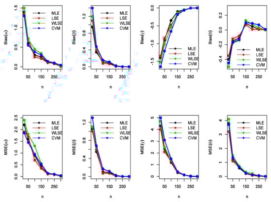
Figure 3. The MSEs and bias estimates of the EGIG for some values of $n$ when $(\alpha$, $\beta$, $\gamma$, $\theta )=\left(1.1, 4.2, 3.5, 0.9\right).$

5.2. Simulation Study 2

As in the first simulation, the simulation replication number was n = 300. The sample sizes used are: $n=20, 50, 100, 150, 200, 250 ,$ and $300$. The parameter values are $(\alpha$, $\beta$, $\gamma$, $\theta )=\left(1.5, 6.1, 3.8, 0.8\right).$ Figure 4 gives the simulation results, which verify the same result obtained with the first simulation. This indicates that the MLE, LSE, WLSE, and CVME approaches perform quite well in estimating the EGIG model parameters.

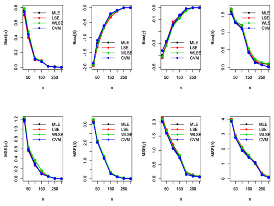
Figure 4. The MSEs and bias estimates of the EGIG for some values of $n$ when $(\alpha$, $\beta$, $\gamma$, $\theta )=\left(1.5, 6.1, 3.8, 0.8\right).$

6. Data Analysis

The empirical importance of the EGIG model is illustrated and discussed in this section, using four different applications to complete actual and upper record data. Our model is compared here with nine other various competitive lifetime models; namely, inverted Weibull (IW), exponentiated generalized inverted Weibull (EGIW), inverted exponential (IE), inverted Rayleigh (IR), inverted flexible Weibull (IFW), exponentiated inverted flexible Weibull (EIFW), A, EGA, and IG distributions. The fitted distributions are compared using some different criteria, such as the log-likelihood values (–L), Anderson-Darling (A*) statistic and Cramér-von Mises (W*) statistic. In addition to the Kolmogorov-Smirnov (KS) statistic, the corresponding p-values are also computed. The MLEs, LSEs, WLSEs, CVMEs, KS, and their p-values will be obtained for the EGIG to compare the four estimation methods with each set of data. Finally, the likelihood ratio test (LRT) is conducted here to examine if the fitting using EGIG is statistically superior to the fitting by the models A, IG, and EGA with the complete data sets.

6.1. Data Set I

The real data mentioned here are studied in [26], and they give the strength of glass for a sample of thirty-one aircraft windows. These data are listed below.

18.83	20.8	21.657	23.03	23.23	24.05	24.321	25.5	25.52	25.8	26.69
26.77	26.78	27.05	27.67	29.9	31.11	33.2	33.73	33.76	33.89	34.76
35.75	35.91	36.98	37.08	37.09	39.58	44.045	45.29	45.381

The MLEs, K-S, corresponding p-values, and the goodness of fit measures are mentioned in Table 1 for all fitted distributions. We find that the EGIG model with the four-parameters $\alpha ,$ $\beta ,$ $\gamma ,$ and $\theta$ has the lowest K-S value and the highest p-value. Furthermore, the goodness of fit measures –L, A*, and W* are the smallest for the EGIG model. This means that the EGIG appears to be a highly competitive lifetime model to the first data set when it is compared with the other nine various lifetime models.

Table 1. The MLEs, K-S, p-values, –L, A*, and W* values for the first data set.

Statistics	Models
	IW	EGIW	IE	IR	IFW	EIFW	A	EGA	IG	EGIG
$\widehat{\alpha }$	4.46 $\times {10}^6$	34.756	29.215	810.504	61.167	2.376	125.662	––	1.249	64.009
$\widehat{\beta }$	4.655	0.637	––	––	0.086	0.164	––	9.526	119.762	63.247
$\widehat{\gamma }$	––	94.688	––	––	––	81.512	––	3.909	––	37.998
$\widehat{\theta }$	––	3.759	––	––	––	––	––	1.95$\times {10}^5$	––	0.18
K-S	0.146	0.124	0.477	0.325	0.146	0.136	0.162	0.145	0.139	0.123
p-value	0.482	0.678	<0.001	0.002	0.479	0.567	0.354	0.485	0.538	0.690
–L	105.323	104.102	137.262	118.201	104.963	104.141	107.95	105.615	107.884	103.286
W*	0.083	0.077	0.074	0.075	0.078	0.074	0.122	0.085	0.118	0.056
A*	0.503	0.407	0.392	0.403	0.467	0.397	0.804	0.521	0.778	0.309

Figure 5 shows the nonparametric Kernel density estimation (KDE) plot, the box plot, the total time test (TTT) plot, and the quantile–quantile (Q–Q) plot. The initial shape of data set I can be explored by the KDE plot, and it is noted that the KDE plot for data set I appears to be nearly symmetric. The extreme values of data set I can be explored by the box plot, and it is noted that no extreme values were found, and the Q–Q plot emphasizes this result. The empirical HRF of data set I can be explored by the TTT plot, and it is noted that the empirical HRF appears to be monotonically increasing. Figure 6 gives the estimated PDF, probability–probability (P–P) plot, estimated CDF, and estimated survival function (SF) for the first data set. Table 2 presents the MLE, LSE, WLSE, and CVM estimators, K-S test statistic and the p-values for the EGIG, and it is found that the WLSE method is the best one to estimate the EGIG parameters because it has the smallest K-S value and the largest p-value. Figure 7 introduces the estimated PDFs, estimated CDFs, and the estimated SFs for the first data set using the estimators in Table 2. The values of the LRT ($\mathsf{\Lambda }$), degree of freedom ($d.f$), and the corresponding p-values for the first data set are presented in Table 3. According to the p-values, it is clear that the null hypothesis ($H_0$) is rejected at $\alpha =0.05$.

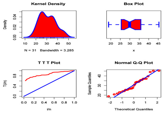
Figure 5. The KDE plot, box plot, TTT plot, and Q–Q plot for the data set I.

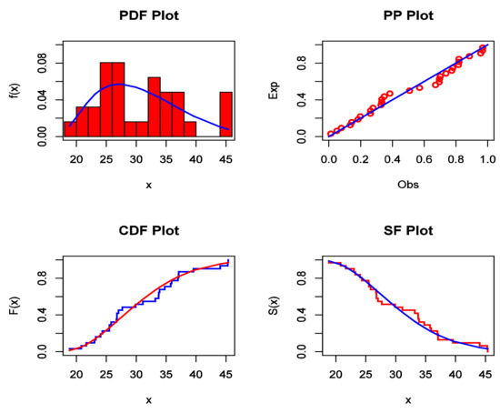
Figure 6. The estimated PDF, P–P plot, estimated CDF, and estimated SF for data set I.

Table 2. The MLE, LSE, WLSE and CVM estimators, KS, and p-values for data set I.

Method	$\widehat{\mathit{\alpha }}$	$\widehat{\mathit{\beta }}$	$\widehat{\mathit{\gamma }}$	$\widehat{\mathit{\theta }}$	K-S	p-Value
MLE	64.009	63.247	37.998	0.180	0.123	0.690
LSE	94.141	54.489	63.339	0.145	0.094	0.945
WLSE	91.462	55.085	63.959	0.147	0.090	0.963
CVM	89.188	56.341	64.313	0.149	0.098	0.929

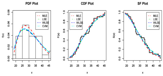
Figure 7. The estimated PDFs, the estimated CDFs, and the estimated SFs for data I.

Table 3. The LRT, $d.f$, and p-values for data set I.

Models	Null Hypothesis $({\mathit{H}}_0)$	$\mathit{\Lambda }$	$\mathit{d}.\mathit{f}$	p-Value
A	$\alpha =\gamma =\theta =1$ or $x_1,x_2,\dots ,x_n~A\left(\beta \right)$	9.328	3	0.025
IG	$\gamma =\theta =1$ or $x_1,x_2,\dots ,x_n~IG\left(\alpha , \beta \right)$	9.196	2	0.010
EGA	$\alpha =1$ or $x_1,x_2,\dots ,x_n~EGA\left(\beta , \gamma , \theta \right)$	4.658	1	0.031

6.2. Data Set II

This data is presented by [27] and they describes the tiredness lifetime of 101 6061-T6 aluminum coupons. It is given as

70	90	96	97	99	100	103	104	104	105	107	152
112	113	114	114	114	116	119	120	120	120	121	174
124	128	128	129	129	130	130	130	131	131	131	109
134	134	134	134	134	136	136	137	138	138	138	124
142	142	142	142	144	144	145	146	148	148	149	132
157	157	157	158	159	162	163	163	164	166	166	141
109	124	132	142	156	212	112	124	133	142	157	155
108	121	131	139	151	168	108	123	131	139	151	196
170	108	124	132	141

Table 4 gives the MLEs, K-S, p-values, and the goodness of fit measures for the mentioned models. The EGIG model has the highest p-value and the lowest K-S value, and also the goodness of fit measures are the smallest for it. This means that EGIG is the best lifetime model to represent the second data set than the nine tested models. Figure 8 gives the KDE plot, the box plot, the TTT plot, and the Q–Q plot. The initial shape of data set II can be explored by the KDE plot, and it is noted that the KDE plot for data set II appears to be nearly symmetric. The extreme values of data set II can be explored by the box plot, and it is noted that some extreme values were found, and the Q–Q plot emphasizes this result. The empirical HRF of data set II can be explored by the TTT plot, and it is noted that the empirical HRF appears to be monotonically increasing.

Table 4. The MLEs, K-S, p-values, –L, A*, and W* values for the second data set.

Statistics	Models
	IW	EGIW	IE	IR	IFW	EIFW	A	EGA	IG	EGIG
$\widehat{\alpha }$	3.28$\times {10}^{10}$	106.236	129.933	1.64$\times {10}^4$	295.466	78.792	705.55	––	7.435	469.618
$\widehat{\beta }$	5.051	0.935	––	––	0.021	0.039	––	94.472	501.775	175.869
$\widehat{\gamma }$	––	11.981	––	––	––	58.724	––	3.041	––	258.604
$\widehat{\theta }$	––	77.271	––	––	––	––	––	6.17$\times {10}^5$	––	0.375
K-S	0.133	0.125	0.506	0.403	0.139	0.113	0.366	0.186	0.206	0.067
p-value	0.055	0.085	< 0.001	< 0.001	0.039	0.153	< 0.001	0.002	< 0.001	0.749
–L	475.186	466.602	595.547	530.197	476.101	465.265	517.597	482.509	494.448	458.896
W*	0.432	0.299	0.121	0.172	0.437	0.238	1.204	0.491	0.803	0.089
A*	2.493	1.694	0.689	0.975	2.548	1.349	7.025	2.851	4.707	0.593

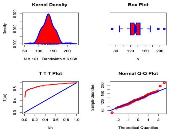
Figure 8. The KDE plot, box plot, TTT plot, and Q–Q plot for data set II.

Figure 9 introduces the estimated PDF, the P–P plot, estimated CDF and estimated SF for data II. Table 5 presents the MLE, LSE, WLSE, and CVM estimators, K-S test statistic, and the p-values for the EGIG, and it is found that the WLSE method is the best one to estimate the EGIG parameters because it has the lowest K-S value and the largest p-value. Figure 10 gives the estimated PDFs, estimated CDFs, and the estimated SFs for data set II using the estimators in Table 5. The values of LRT, $d.f,$ and the p-values for data set II are given in Table 6. Based on the p-values, the null hypotheses are rejected at $\alpha =0.05.$

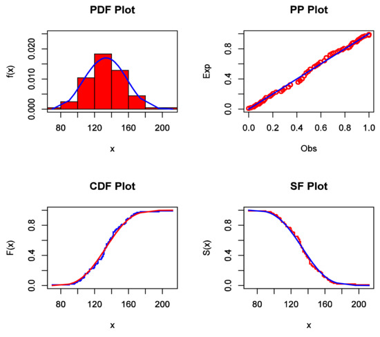
Figure 9. The estimated PDF, P–P plot, estimated CDF, and estimated SF for data set II.

Table 5. The MLE, LSE, WLSE, and CVM estimators, K-S, and p-values for data set II.

Method	$\widehat{\mathit{\alpha }}$	$\widehat{\mathit{\beta }}$	$\widehat{\mathit{\gamma }}$	$\widehat{\mathit{\theta }}$	K-S	p-Value
MLE	469.618	175.869	258.604	0.375	0.067	0.749
LSE	515.696	121.802	225.434	0.632	0.057	0.897
WLSE	397.808	172.611	141.765	0.529	0.057	0.904
CVM	490.022	134.638	218.369	0.600	0.072	0.666

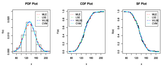
Figure 10. The estimated PDFs, the estimated CDFs, and the estimated SFs for data set II.

Table 6. The LRT, $d.f,$ and p-values for data set II.

Models	Null Hypothesis $({\mathit{H}}_0)$	$\mathit{\Lambda }$	$\mathit{d}.\mathit{f}$	p-Value
A	$\alpha =\gamma =\theta =1$ or $x_1,x_2,\dots ,x_n~A\left(\beta \right)$	117.402	3	0.0
IG	$\gamma =\theta =1$ or $x_1,x_2,\dots ,x_n~IG\left(\alpha , \beta \right)$	71.104	2	0.0
EGA	$\alpha =1$ or $x_1,x_2,\dots ,x_n~EGA\left(\beta , \gamma , \theta \right)$	47.226	1	0.0

6.3. Data Set III

The actual data introduced here are offered by [28] and they represents the simulated strengths for a sample of 63 glass fibers. These data are given as

1.014	1.081	1.082	1.185	1.223	1.248	1.267	1.271	1.748
1.288	1.292	1.304	1.306	1.355	1.361	1.364	1.379	3.197
1.481	1.484	1.501	1.506	1.524	1.526	1.535	1.541	1.276
1.602	1.666	1.670	1.684	1.691	1.704	1.731	1.735	1.459
1.867	1.876	1.878	1.910	1.916	1.972	2.012	2.456	1.581
1.278	1.460	1.591	1.800	1.286	1.476	1.593	1.806	1.757
1.272	1.409	1.568	1.747	2.592	1.275	1.426	1.579	4.121

The MLEs, K-S, p-values, and the goodness of fit statistics are listed for all tested models in Table 7. The EGIG model has the highest p-value and the lowest K-S value, and also the goodness of fit statistics are the smallest for it. This confirms that EGIG is the best lifetime model to represent the third data set among the tested models. The KDE plot, the box plot, the TTT plot, and the Q–Q plot are presented in Figure 11. The initial shape of data set III can be explored by the KDE plot, and it is noted that the KDE plot for data set III appears to be asymmetrically right-skewed with a heavy tail. The extreme values of data set III can be explored by the box plot, and it is noted that some extreme values were found, and the Q–Q plot emphasizes this result. The empirical HRF of data set III can be explored by the TTT plot, and it is noted that the empirical HRF appears to be monotonically increasing. Figure 12 shows the estimated PDF, P–P plot, estimated CDF, and estimated SF for the current data. Table 8 introduces the MLE, LSE, WLSE, and CVM estimators, K-S test statistic, and the p-values for EGIG, and it is found that the LSE method is the best one to estimate the EGIG parameters because the LSE method has the lowest K-S value, and also the highest p-value. Figure 13 gives the estimated PDFs, estimated CDFs, and the estimated SFs for data set III using the estimators in Table 8. The values of LRT, $d.f,$ and the p-values for data set III are introduced in Table 9, and it is obvious that $H_0$ is rejected at $\alpha =0.05.$ From Table 7, we notice that the value of W* for the EGA model (0.059) is smaller than the value of W* for EGIG model (0.061). Moreover, the p-value for the EGA model mentioned in Table 9 is more than $0.05$, this means that $H_0$ is not rejected with this model. This result confirms that the EGA model is also suitable to describe data set III as well as our proposed model.

Table 7. The MLEs, K-S, p-values, –L, A*, and W* values for the third data set.

Statistics	Models
	IW	EGIW	IE	IR	IFW	EIFW	A	EGA	IG	EGIG
$\widehat{\alpha }$	6.498	1.161	1.526	2.233	3.732	4.169	2.111	––	0.032	0.495
$\widehat{\beta }$	5.438	3.529	––	––	1.869	1.666	––	1.54	7.583	3.761
$\widehat{\gamma }$	––	1.731	––	––	––	0.544	––	6.249	––	3.656
$\widehat{\theta }$	––	8.139	––	––	––	––	––	7.331	––	1.461
K-S	0.077	0.071	0.468	0.36	0.082	0.084	0.521	0.069	0.101	0.068
p-value	0.819	0.889	<0.001	<0.001	0.756	0.739	<0.001	0.904	0.508	0.916
–L	20.064	19.879	92.805	53.381	20.618	20.593	63.322	19.913	22.809	19.706
W*	0.071	0.062	0.126	0.087	0.079	0.081	0.063	0.059	0.138	0.061
A*	0.533	0.488	0.982	0.709	0.61	0.616	0.514	0.482	0.928	0.469

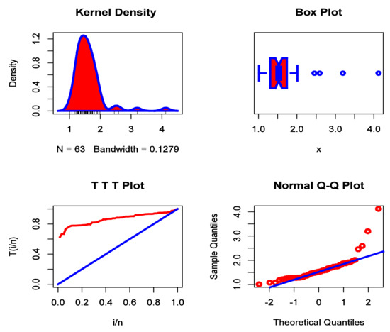
Figure 11. The KDE plot, box plot, TTT plot, and Q–Q plot for data set III.

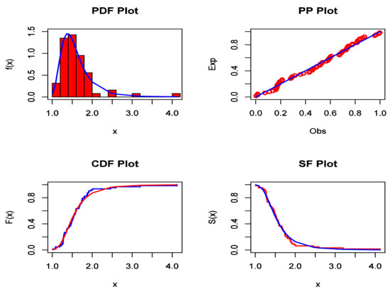
Figure 12. The estimated PDF, P–P plot, estimated CDF, and the estimated SF for data set III.

Table 8. The MLE, LSE, WLSE, and CVM estimators, KS, and p-values for data set III.

Method	$\widehat{\mathit{\alpha }}$	$\widehat{\mathit{\beta }}$	$\widehat{\mathit{\gamma }}$	$\widehat{\mathit{\theta }}$	K-S	p-Value
MLE	0.495	3.761	3.656	1.461	0.068	0.916
LSE	0.596	3.278	4.339	1.999	0.067	0.927
WLSE	0.847	2.722	5.856	2.369	0.075	0.866
CVM	0.589	3.300	4.363	2.031	0.072	0.898

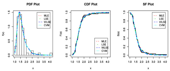
Figure 13. The estimated PDFs, the estimated CDFs, and the estimated SFs for data set III.

Table 9. The LRT, $d.f,$ and p-values for data set III.

Models	Null Hypothesis $({\mathit{H}}_0)$	$\mathit{\Lambda }$	$\mathit{d}.\mathit{f}$	p-Value
A	$\alpha =\gamma =\theta =1$ or $x_1,x_2,\dots ,x_n~A\left(\beta \right)$	87.232	3	0.0
IG	$\gamma =\theta =1$ or $x_1,x_2,\dots ,x_n~IG\left(\alpha , \beta \right)$	6.206	2	0.045
EGA	$\alpha =1$ or $x_1,x_2,\dots ,x_n~EGA\left(\beta , \gamma , \theta \right)$	0.414	1	0.519

6.4. Data Set V (Upper Record Data)

In some applications, such as meteorology, seismology, economics, and athletic events, the record values have an extensive importance. The upper record value can be defined as the value that is bigger than all observed values yet. If $x_1,x_2,\dots , x_n$ is a random sample from $\mathrm{EGIG}\left(\Omega \right)$ and $X=\left\{X_{U\left(1\right)},X_{U\left(2\right)}, \dots ,X_{U\left(n\right)}\right\}$ are the upper record values taken from it, then the likelihood function of $X$ is obtained by the formula (see [29])

$${\ell }_{reco.}=f\left(x_{U\left(n\right)};\Omega \right){\displaystyle \prod }_{i=1}^{n-1}\frac{f\left(x_{U\left(i\right)}, \Omega \right)}{R\left(x_{U\left(i\right)}, \Omega \right)}, 0\le x_{U\left(1\right)}<x_{U\left(2\right)}<\dots <x_{U\left(n\right)}<\infty .$$

(35)

Substituting from Equations (6) and (7) into Equation (35), the $L\left(\Omega \right)$ of $X$ will be

$$\begin{array}{cc}L\left(\Omega \right)=& nln\left(\mathsf{\alpha }\gamma \theta \right)-\ln \left(x_{U\left(n\right)}^2\right)+\frac{\beta }{x_{U\left(n\right)}}-\frac{\alpha }{\beta }\left(e^{\frac{\beta }{x_{U\left(n\right)}}}-1\right)+\left(\gamma -1\right)\ln \left(1-e^{\frac{-\alpha }{\beta }\left(e^{\frac{\beta }{x_{U\left(n\right)}}}-1\right)}\right)\hfill \\ & +\left(\theta -1\right)\ln \left[1-{\left(1-e^{\frac{-\alpha }{\beta }\left(e^{\frac{\beta }{x_{U\left(n\right)}}}-1\right)}\right)}^{\gamma }\right]-{\displaystyle \sum }_{i=1}^{n-1}\ln \left(x_{U\left(i\right)}^2\right)+\beta {\displaystyle \sum }_{i=1}^{n-1}\frac{1}{x_{U\left(i\right)}}-\frac{\alpha }{\beta }{\displaystyle \sum }_{i=1}^{n-1}\left(e^{\frac{\beta }{x_{U\left(i\right)}}}-1\right)\hfill \\ & +\left(\gamma -1\right){\displaystyle \sum }_{i=1}^{n-1}\ln \left(1-e^{\frac{-\alpha }{\beta }\left(e^{\frac{\beta }{x_{U\left(i\right)}}}-1\right)}\right)+\left(\theta -1\right){\displaystyle \sum }_{i=1}^{n-1}\ln \left[1-{\left(1-e^{\frac{-\alpha }{\beta }\left(e^{\frac{\beta }{x_{U\left(i\right)}}}-1\right)}\right)}^{\gamma }\right]\hfill \\ & -{\displaystyle \sum }_{i=1}^{n-1}\ln \left\{1-{\left[1-{\left(1-e^{\frac{-\alpha }{\beta }\left(e^{\frac{\beta }{x_{U\left(i\right)}}}-1\right)}\right)}^{\gamma }\right]}^{\theta }\right\}.\hfill \end{array}$$

(36)

By differentiating Equation (36) for $\alpha , \beta , \gamma ,$ and $\theta$ and equating it to zero, we will obtain a non-linear system of equations that are solved numerically to find $\widehat{\alpha }, \widehat{\beta }, \widehat{\gamma },$ and $\widehat{\theta }.$ The record data studied here are mentioned by [30] and represents the lifetimes to breakdown for a sample of 11 electric isolating fluids exposed to 30 kilovolts. The data considered here are 2.836, 3.120, 3.045, 5.169, 4.934, 4.970, 3.018, 3.770, 5.272, 3.856, and 2.046. The upper record values of these data are 2.836, 3.120, 5.169, and 5.272. The MLEs, –L, KS, and p-values for the A, IG, EGA, and EGIG distributions are listed in Table 10. The EGIG has the smallest –L and K-S values and the largest p-value, and this result confirms that the EGIG fits data set V better than the A, IG and EGA models.

Table 10. The MLEs, –L, K-S, and p-values for data set V.

Models	MLEs	–L	K-S	p-Value
A	$\widehat{\alpha }=7.136$	7.592	0.687	0.046
IG	$\widehat{\alpha }=2.82\times {10}^{-3}, \widehat{\beta }=26.399$	3.25	0.513	0.285
EGA	$\widehat{\beta }=9.598, \widehat{\gamma }=4.062, \widehat{\theta }=0.655$	2.992	0.479	0.319
EGIG	$\widehat{\alpha }=1.409, \widehat{\beta }=13.086, \widehat{\gamma }=4.178, \widehat{\theta }=0.112$	2.873	0.469	0.341

7. Conclusions

This article studied and proposed a lifetime model with four parameters, shortly EGIG, which is considered as an extension to the inverted Gompertz distribution. The EGIG is capable of modeling the lifetimes with upside-down bathtub-shaped HRF and is suitable to describe the negative and positive skewness in addition to the symmetric data sets. Furthermore, the EGIG is convenient for testing the goodness of fit of three special sub-models, the A, IG, and EGA models. Some distributional properties of the EGIG are derived and discussed, such as the PDF, CDF, SF, HRF, reversed HRF, quantile function and median, moments (PWMs), entropy function, MWT and MRL, and others. The parameters of the EGIG are estimated by using four various estimation methods. A simulation study is carried out to examine and study the performance of the MLEs, LSEs, WLSEs, and CVMEs according to both the MSEs and biases. The simulation results supported that the four estimation methods performed quite well when estimating the EGIG parameters. The empirical significance of the EGIG model is clarified using three complete data sets, symmetric and asymmetric, from engineering and it is compared with nine other various competitive lifetime models. The EGIG model can be used quite effectively to give better fits than the nine other tested lifetime models. Moreover, our model is compared with the A, IG, and EGA models for the upper record data. Finally, we hope that the suggested model (EGIG) will serve a lot of applications in reliability, engineering, and others.

References

- Gompertz, B. On the nature of the function expressive of the law of human mortality, and on a new mode of determining the value of life contingencies. Philos. Trans. R. Soc. Lond. 1825, 115, 513–583. [Google Scholar]
- Read, C.B. Gompertz distribution. Encyclopedia of Statistical Sciences; Wiley: New York, NY, USA, 1983. [Google Scholar]
- Franses, P.H. Fitting a Gompertz curve. J. Oper. Res. Soc. 1994, 45, 109–113. [Google Scholar] [CrossRef]
- Chen, Z. Parameter estimation of the Gompertz population. Biom. J. 1997, 39, 117–124. [Google Scholar] [CrossRef]
- Wu, J.W.; Lee, W.C. Characterization of the mixtures of Gompertz distributions by conditional expectation of order statistics. Biom. J. 1999, 41, 371–381. [Google Scholar] [CrossRef]
- El-Gohary, A.; Alshamrani, A.; Al-Otaibi, A.N. The generalized Gompertz distribution. Appl. Math. Model. 2013, 37, 13–24. [Google Scholar] [CrossRef] [Green Version]
- Jafari, A.; Saeid, T.; Morad, A. The beta-Gompertz distribution. Colomb. J. Stat. (Rev. Colomb. De Estad.) 2014, 37, 139–156. [Google Scholar] [CrossRef] [Green Version]
- Khan, M.S.; Robert, K.; Irene, L.H. Transmuted Gompertz distribution: Properties and estimation. Pak. J. Stat. 2016, 32, 161–182. [Google Scholar]
- Eliwa, M.S.; El-Morshedy, M.; Ibrahim, M. Inverse Gompertz distribution: Properties and different estimation methods with application to complete and censored data. Ann. Data Sci. 2019, 6, 321–339. [Google Scholar] [CrossRef]
- Alshenawy, R. A new one parameter distribution: Properties and estimation with applications to complete and type II censored data. J. Taibah Univ. Sci. 2020, 14, 11–18. [Google Scholar] [CrossRef] [Green Version]
- El-Morshedy, M.; El-Faheem, A.A.; El-Dawoody, M. Kumaraswamy inverse Gompertz distribution: Properties and engineering applications to complete, type-II right censored and upper record data. PLoS ONE 2020, 15(12), e0241970. [Google Scholar] [CrossRef]
- Cordeiro, G.M.; de Castro, M. A new family of generalized distributions. J. Stat. Comput. Simul. 2011, 81, 883–898. [Google Scholar] [CrossRef]
- Zografos, K.; Balakrishnan, N. On families of beta-and generalized gamma-generated distributions and associated inference. Stat. Methodol. 2009, 6, 344–362. [Google Scholar] [CrossRef]
- Alexander, C.; Cordeiro, G.M.; Ortega, E.M.M.; Sarabia, J.M. Generalized beta generated distributions. Comput. Stat. Data Anal. 2012, 56, 1880–1897. [Google Scholar] [CrossRef]
- Ristic, M.M.; Balakrishnan, N. The Gamma-exponentiated Exponential Distribution. J. Stat. Comput. Simul. 2012, 82, 1191–1206. [Google Scholar] [CrossRef]
- Amini, M.; MirMostafaee, S.M.T.K.; Ahmadi, J. Log-gamma-generated families of distributions. Statistics 2012, 48, 913–932. [Google Scholar] [CrossRef]
- Alzaatreh, A.; Lee, C.; Famoye, F. A new method for generating families of continuous distributions. Metron 2013, 71, 63–79. [Google Scholar] [CrossRef] [Green Version]
- Cordeiro, G.M.; Ortega, E.M.M.; da Cunha, D.C.C. The exponentiated generalized class of distributions. J. Data Sci. 2013, 11, 1–27. [Google Scholar] [CrossRef]
- El-Bassiouny, A.H.; El-Morshedy, M. The univarite and multivariate generalized slash student distribution. Int. J. Math. Its Appl. 2015, 3, 35–47. [Google Scholar]
- Tahir, M.H.; Cordeiro, G.M.; Alzaatreh, A.; Mansoor, M.; Zubair, M. The logistic-X family of distributions and its applications. Commun. Stat.-Theory Methods 2016, 45, 7326–7349. [Google Scholar] [CrossRef] [Green Version]
- Eliwa, M.S.; El-Morshedy, M.; Afify, A.Z. The odd Chen generator of distributions: Properties and estimation methods with applications in medicine and engineering. J. Natl. Sci. Found. 2020, 48, 1–23. [Google Scholar] [CrossRef]
- Zaidi, S.M.; Sobhi, M.M.A.; El-Morshedy, M.; Afify, A.Z. A new generalized family of distributions: Properties and applications. AIMS Math. 2020, 6, 456–476. [Google Scholar] [CrossRef]
- Altun, E.; Korkmaz, M.C.; El-Morshedy, M.; Eliwa, M.S. The extended gamma distribution with regression model and applications. AIMS Math. 2021, 6, 2418–2439. [Google Scholar] [CrossRef]
- Kenney, J.; Keeping, E. Mathematics of Statistics, 3rd ed; Van Nostrand Company: Canada, 1962; Volume 1. [Google Scholar]
- Moors, J.J.A. A quantile alternative for kurtosis. J. R. Stat. Soc. Ser. D (Stat.) 1988, 37, 25–32. [Google Scholar] [CrossRef] [Green Version]
- Fuller, E.J.; Frieman, S.; Quinn, J.; Quinn, G.; Carter, W. Fracture mechanics approach to the design of glass aircraft windows: A case study. SPIE Proc. 1994, 2286, 419–430. [Google Scholar]
- Birnbaum, Z.W.; Saunders, S.C. Estimation for a family of life distributions with applications to fatigue. J. Appl. Probab. 1969, 6, 328–347. [Google Scholar] [CrossRef]
- Mahmoud, M.R.; Mandouh, R.M. On the transmuted fréchet distribution. J. Appl. Sci. Res. 2013, 9, 5553–5561. [Google Scholar]
- Arnold, B.C.; Balakrishnan, N.; Nagaraja, H.N. Records; John Wiley: New York, NY, USA, 1998. [Google Scholar]
- Lawless, J.F. Statistical Models and Methods for Lifetime Data, 2nd ed.; Wiley: New York, NY, USA, 1982. [Google Scholar]
Publisher’s Note: MDPI stays neutral with regard to jurisdictional claims in published maps and institutional affiliations. |
© 2021 by the authors. Licensee MDPI, Basel, Switzerland. This article is an open access article distributed under the terms and conditions of the Creative Commons Attribution (CC BY) license (https://creativecommons.org/licenses/by/4.0/).