Abstract
A two-dimensional numerical model for solving the Navier–Stokes equations was developed to investigate the local scour around a submarine pipeline with a spoiler. Both the suspended load and the bed load were considered in the present numerical model. The focus of the present study is to investigate the effects of the spoiler length on the hydrodynamic forces on the pipeline and the spoiler as well as the local scour around the submarine pipeline. The corresponding numerical results show that the mean drag coefficients of the pipeline and the spoiler increase with the increase of the spoiler length. As for the mean lift coefficient, a general decreasing trend with the increasing spoiler length is observed for the pipeline. However, the mean lift coefficient of the spoiler first increases and then decreases with the increasing spoiler length. In addition, it is found that a larger spoiler length leads to a deeper scour depth, and an empirical equation was proposed for predicting the non-dimensional scour depth of submarine pipelines with non-dimensional spoiler length based on the numerical results.
1. Introduction
Submarine pipelines, the lifeline of the offshore petroleum engineering, are widely used in recent decades. When a pipeline is laid on an erodible seabed, the presence of the pipeline will change the flow structures around it, resulting in an amplification effect on the bed shear stress. When the bed shear stress is larger than the threshold shear stress of the sediment, the sediment beneath and around the pipeline will be taken away by the flow, then local scour occurs. The pipeline may lose its on-bottom stability and experience the resultant failure due to the local scour. Hence, it is important to study the features of the local scour around submarine pipelines and develop design solutions to protect pipelines induced by the local scour accordingly.
Many researchers have carried out various studies on different aspects of the local scour around submarine pipelines. Two methods are generally employed in these studies: physical experiments and numerical simulations. Research work [1] found that the local scour depth beneath the submarine pipelines increases first with the increase of the incoming flow velocity until the local scour depth attains its maximum value at a certain flow velocity. After that, the local scour depth decreases with the further increase in the incoming flow velocity [1]. This flow velocity, at which the local scour depth reaches its maxima, is defined as the critical velocity [1]. Through an experimental study, it is pointed out that both the diameter of the pipeline and the incoming flow velocity have significant effects on the local scour around submarine pipelines [2]. Another experimental study on local scouring of submarine pipelines with various initial burial depths was carried out by [3] and it is found that the equilibrium scouring depth decreases with the increase of the non-dimensional burial depth (i.e., the ratio between the initial burial depth and the pipeline diameter). According to the experimental results of [4], the local scour problem can be divided into two categories: namely the clear water scour (θ < θcr0) and the dynamic bed scour (θ > θcr0) (θ is the Shields parameter; θcr0 is the critical Shields parameter). For these two scouring types, further experimental studies were carried out by [5] under steady current conditions. The results show that in the case of the clear water scour, the scour depth approximately increases monotonously with the increase of the shields parameter. The maximum scour depth occurs when θ = θcr0. For the case of the dynamic bed scouring problem, the variation of the scour depth with the Shields parameter becomes non-linear. It is found that the scour depth first decreases with the Shields parameter and then increases with its further increase. However, the scour depth stays approximately constant and is independent on the increasing Shields parameter.
In addition to experimental studies, numerical simulations are also a powerful method to study the local scour around pipelines. Local scour around submarine pipelines under steady currents was investigated by [6] using a potential flow model. It was found that the potential model is able to predict the maximum scour depth beneath the pipeline reasonably. However, the simulation results associated with the scour profile around the pipeline are significantly different from the experimental measurements. Further examinations showed that the potential model cannot capture the vortex shedding behind the pipeline, and thus leads to this discrepancy between the potential solutions and the experimental results [7]. To resolve the problem mentioned above, a viscous flow model solving the Navier–Stokes equations was developed [8]. In the work conducted by [8], a concept of bottom shear stress balance was introduced to simulate the equilibrium profile of local scour. The corresponding results show that the simulated equilibrium scour profiles were consistent with the experimental observations. However, the development of the local scour with time was not captured properly by this viscous flow model. Subsequently, a new local scour model was developed by [9]. Similar to the work of [8], the Navier–Stokes equations were also solved to obtain the detailed flow structure, while the seabed change induced by the local scour is achieved by solving the equation of the sediment mass conservation by considering both the suspended load and the bed load. The corresponding results showed that the newly developed numerical model is capable of describing the development of scour profiles over time, and then the validated numerical model was used to simulate the local scour around a sagging pipeline at different sagging speeds. After that, further numerical studies were carried out to investigate the local scour around a vibrating pipeline under the action of unidirectional flow [10,11].
However, fewer research results, considering the numerical study of the local scour around submarine pipelines under wave actions, are available in the literature. Representative research is the numerical study considering an oscillatory flow developed by [12]. In this numerical model, the wave motion is simplified into an oscillatory flow and the effect of the free water surface on the local scour of a pipeline is ignored. Comparing the numerical results and the experimental measurements in [13], it is shown that the simplified oscillatory flow model is able to give reasonable predictions of local scour around the pipeline. However, it should be noted here that when the wave non-linearity is significant, the ignorance of the free water surface may result in large errors, as the oscillatory flow model assumes a strictly horizontal symmetry of the water particle motion. This assumption is no longer valid when the symmetry is broken due to, e.g., the significant wave non-linear features or waves propagating on an uneven seabed. For these problems, the numerical model, which can consider the effect of wave free surface, should be used, for example the work conducted by [14], which investigates the effect of the free water surface on the local scour around a submarine pipeline. After that, the local scour around submarine pipelines under various wave and seabed slope conditions was further investigated in [15]. The numerical results of the equilibrium scour depth agree well with those calculated by the empirical formula proposed by [13] when KC < 8, while there is a discrepancy between the results calculated by the numerical model and the empirical formula when KC ≥ 8; a larger value is obtained by the numerical model. The KC number here is defined as KC = UT/D with U being the amplitude of the wave velocity, T being the wave period and D being the pipeline diameter.
A so-called phenomenon of the self-burial may occur in which the pipeline is buried by the sediments moved from beneath the pipeline by the local scour. Obviously, the self-burial would enhance the on-bottom stability of the submarine pipelines. Thus, lots of methods were developed in attempt to promote the local scour, hence, triggering the self-burial. The spoiler, a vertical plate placed on top of a pipeline, has been developed to increase the local scour. In addition, the spoiler can protect the submarine pipeline by avoiding the damages from human activities such as fishing gear. Numerical simulations were performed to study the flow field around a pipeline with a spoiler near a rigid bed using ANSYS [16]. The result showed that the k-ω turbulence model works well at simulating this complex flow field. An experiment was conducted to study the scour depth for a submarine pipeline with a spoiler [17]. The experimental results revealed that the scour depth beneath a submarine pipeline is dependent on the spoiler length. Both experimental and numerical studies were carried out to investigate the self-burial mechanism of a pipeline with a spoiler in a steady current in [18]. It is found that this is mainly due to the fact that the projected area is increased by the spoiler.
In general, for the problem of local sediment scour around submarine pipelines under the action of a flow (e.g., flow current or waves), researchers have obtained abundant research results through experimental and/or numerical methods. However, for the local scour of submarine pipelines with a spoiler, the related numerical analysis is rather limited (at least to the authors’ best knowledge). Hence, numerical simulations were conducted to identify the effects of the spoiler length on the local scour around submarine pipelines and the corresponding hydrodynamic forces, so as to provide a scientific basis and technical reference for the design, construction and safe service of such submarine pipelines.
2. Materials and Methods
2.1. Numerical Model
2.1.1. Flow Governing Equations
The Reynolds-averaged Navier–Stokes (RANS) equations for an incompressible viscous Newtonian fluid from an arbitrary Lagrangian–Eulerian (ALE) point of view can be written in the following form:
where, ui is the velocity component corresponding to the xi direction (u1 = u, u2 = v, x1 = x, x2 = y), and ujm is the velocity of the moving grids corresponding to the xi directions. It should be mentioned here that the movement of the computational grids is induced by the change of the seabed profile due to the local scour. Time is t, p is the pressure, ρ is the fluid density, and υ is the fluid kinematic viscosity coefficient. Sij is the mean strain rate tensor, which is defined as follows:
The last term in Equation (2) is the Reynolds stress, defined as υt(∂ui/∂xj + ∂uj/∂xi) + 2kδij/3, where, υt is the turbulent eddy viscosity, k is the turbulence kinetic energy, and δij is the Kronecker operator. In the present study, the above flow equations are closed using the Shear Stress Transport (SST) k-ω two-equations turbulence model [19,20], which has been proven to be well qualified for simulating the flow structure with a significant adverse pressure gradient. The convective-transport equations for the SST k-ω turbulence model are:
where, k is the turbulence kinetic energy, and its specific dissipation rate is defined as ω.
The definitions of the other relevant variables in the above equations and the values of the constants can be found in the work of [19,20].
2.1.2. Sediment Transport Model
The seabed change induced by the local scour around the submarine pipeline can be described by the following seabed deformation equations:
where yb is the seabed elevation, λs is the porosity of the sediment, qb is the bed load transport rate (obtained by Equation (12)), and qs is the suspended load transport rate, which can be obtained by:
where ys is the height of the free water surface. For the steady current with a symmetry boundary condition imposed on the top of the computational domain, ys equals to the water depth d, c is the concentration of sediment, and ya = 2.0d50 is a reference height of the boundary between suspended and bed load transports, with d50 being the median particle size of the sediment.
The concentration of the sediment c is obtained by the following equation for the diffusion of the suspended mass concentration:
where σc (=1 in this paper) is the Schmidt number of the turbulence, and wsj is the settling velocity of sediment particles. In the x direction, ws1 = 0.0; in the y direction, ws2 is calculated based on the formula developed by [21]:
where m = 5.0, and ws0 is given according to the formula proposed by [21,22]:
where D* is the dimensionless sediment grain size, which is defined as:
where s is the ratio of the sediment density ρs to the fluid density ρ, and g is the acceleration due to gravity.
The bed load transport rate qb was calculated using the following equation developed by [23]:
where the parameter T0 is defined as:
where τ0 is the bottom bed shear stress, θ = τ0/gd50/(ρs-ρ) is the Shields parameter, and θcr is the critical Shields parameter, which is defined as:
where α is the local topographic slope of a seabed, ψ is the sediment rest angle, and θcr0 can be obtained by the empirical formula recommended by [23,24].
2.1.3. Boundary Conditions
For the inlet boundary, the conditions of u = U, v = V = 0 and ∂p/∂n = 0 are imposed, where n is the unit outward normal vector. For the case of the turbulence model at the inlet boundary, the following additional boundary conditions are used at in inlet: k = (0.005Uav)2 and ω = 0.16k0.5/(0.018d) with Uav = (u2 + v2)0.5 being the magnitude of the fluid velocity and d being the water depth. The no-slip boundary conditions are adopted on the surface of the pipeline, i.e., u = 0, v = 0 and ∂p/∂n = 0. The turbulence energy k is set to be zero on the pipeline surface, and ω = 6Δ/υ with Δ being the distance of the first layer meshes adjacent to the pipeline surface to the pipeline surface. The velocities at the outlet are described as ∂ui/∂t + χ∂ui/∂x = 0, where χ is the spatial averaged flow velocity, and the boundary conditions for k and ω are similar to the boundary condition for the fluid velocity at the outlet boundary. Meanwhile, a relative pressure p = 0 is imposed along the outflow boundary for the pressure equation. For the top boundary, a symmetry boundary condition, namely ∂u/∂y = 0, v = 0, and ∂p/∂y = 0, is employed to reduce the size of the computational domain, thus the consequent number of computational meshes. The similar symmetry boundary conditions are also used for the turbulent model, namely ∂k/∂n = 0 and ∂ω/∂n = 0 at the top boundary. To save the computational time, the standard wall function is introduced on the seabed. The first layer of mesh nodes is located at a distance Δ1 away from the seabed, where the logarithmic wall function is applied:
where uτ is the friction velocity, κ is the Karman constant with κ = 0.41, and Δb is the bed roughness which is evaluated as Δb = d50/12. It should be noted here that in the application of the above-mentioned standard wall function, the boundary layer should be able to achieve a state of complete development, and the distribution of the horizontal fluid velocity associated with the water depth should satisfy the logarithmic law, as described by Equation (16). For the SST k-ω model, the turbulent energy k and its specific dissipation rate ω on the first layer of mesh nodes are given as:
where Cu is an empirical coefficient with its value being 0.09.
The boundary condition for the sediment concentration Equation (8) is applied at a reference height (ya = 2.0d50) above the seabed, which is evaluated according to the following equation:
A Streamline Upwind Petrov–Galerkin Finite Element Method (SUPG-FEM) was employed to solve the governing equations mentioned above. The details of the above numerical method can refer to the work of [25] and will not be repeated here. The seabed profile will change with the development of local scour around the submarine pipeline, leading to a moving boundary condition. In the present study, the ALE method was introduced to capture the moving boundary and update the computational meshes at each time step. This method has been proven to be capable of simulating the scour problems, and the details of the ALE method can be seen in our previous work by considering local scour around a submarine pipeline under different wave conditions [14].
2.1.4. Computational Domain and Meshes
Figure 1 gives the sketch of the computational domain in which a submarine pipeline with a diameter of D = 1.0 m is placed on the seabed. A spoiler is placed on the top surface of the submarine pipeline; its length is defined as L. The water depth d is set to be 20 D. The total length of the computational domain is 60 D. A symmetry distribution of the inlet and outlet boundaries is set up in the present numerical model as shown in Figure 1. The distances from the inlet boundary and the outlet boundary to the center of the pipeline are both 30 D.
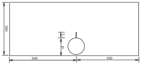
Figure 1.
Sketch of the computational domain.
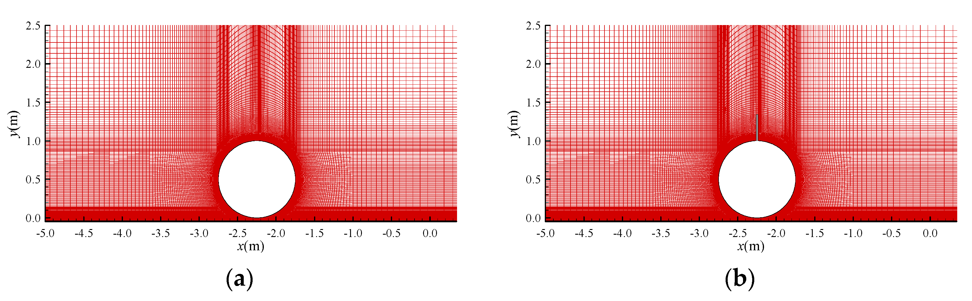
The four-node quadrilateral finite element is used to discretize the computational domain. Figure 2 shows the computational meshes used for the two scenarios considered in the present study, i.e., a smooth pipeline and a pipeline with a spoiler with its length L = 0.33 D. To ensure both the accuracy and the computational efficiency, denser meshes are adopted around the pipelines and coarser meshes are used in the area far away from the pipelines.
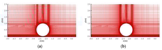
Figure 2.
Two typical meshes around the pipelines: (a) meshes around a smooth pipeline; (b) meshes around a pipeline with a spoiler.
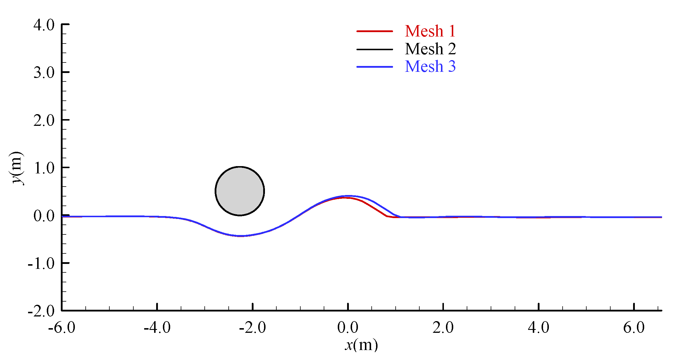
In order to test the mesh convergence, three meshes with various resolutions are used for investigating the local scour around a smooth pipeline; 120, 240 and 360 grids are adopted on the surface of the pipeline, defined as Mesh 1, Mesh 2 and Mesh 3, respectively. The total node numbers in Mesh 1, Mesh 2 and Mesh 3 are 40,116, 58,968 and 68,278, respectively, and the corresponding element numbers are 39,616, 58,356 and 67,636, respectively. Figure 3 gives the scour profile around the pipeline at t = 3000 s. For this time instant, the local scour attains its equilibrium profile. From the comparisons shown in Figure 3, it can be seen that the scour profiles calculated with the Mesh 2 and Mesh 3 are almost the same. Therefore, the Mesh 2 is adopted in this study in order to save the computational resource and time hereafter.
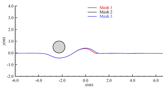
Figure 3.
Scour profile around the pipeline under the three different meshes.
2.2. Validation of the Numerical Model
In this section, the numerical model is validated by comparing the scour profiles with the published experimental data [6]. In the experiment, the local scour around a submarine pipeline in a steady current was studied. In the present numerical simulations, the parameters are consistent with the experimental parameters, as shown in Table 1.

Table 1.
Calculation parameters.
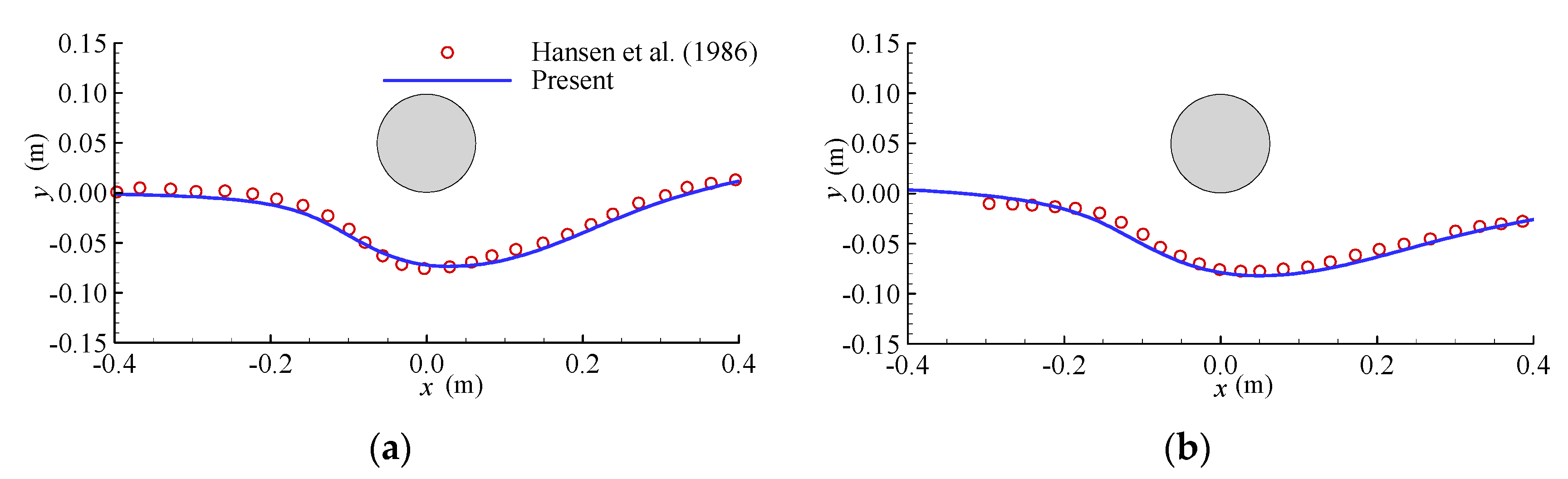
From the comparison of the results shown in the Figure 4, it can be seen that the present numerical results agree well with the experimental results, indicating that the numerical model established by the present study can reliably predict the development process of the local scour and the scour profile around the submarine pipeline. Hence, the validated model can then be used to study the local scour around a pipeline with a spoiler in the following section.
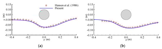
Figure 4.
Scour profile around a pipeline under a steady current at two different instants: (a) t = 30 min and (b) t = 217 min.
In addition, it can also be seen from Figure 4 that there is a difference between the morphology of the scour hole around the pipeline at t = 30 min and that at t = 217 min. The seabed slope behind the pipeline becomes flatter after a longer time as shown in Figure 4b. This is mainly due to the shedding of vortices in the wake zone of the pipeline. This phenomenon cannot be correctly captured by the potential flow model due to the assumption of irrotational flow, as indicated previously.
3. Results
It is well recognized that the spoiler has a significant effect on the local scour around a pipeline. Hence, this section investigates the local scour around submarine pipelines with different spoiler lengths. The parameters used in the numerical simulation are: the water depth d = 20 m, the pipeline diameter D = 1.0 m, the median particle of the sediment d50 = 0.58 mm and the length of the spoiler L = 0.11 m, 0.22 m and 0.33 m. Table 2 gives the details of these parameters.
Table 2.
Parameters for the numerical setup.
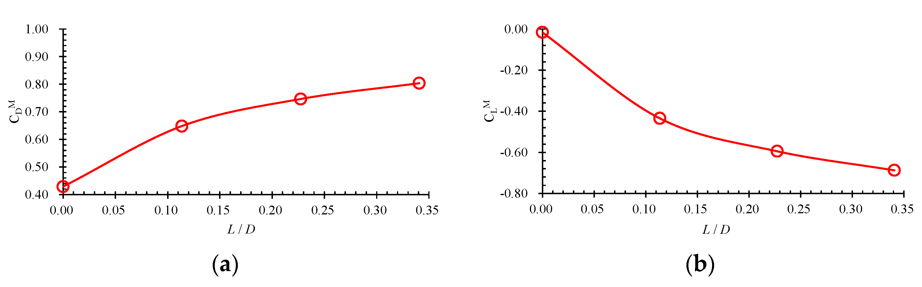
Figure 5 shows the variations of the mean drag and the lift force coefficients (CDM and CLM, respectively) of the submarine pipeline with respect to the spoiler length. In the present study, the time-dependent drag and lift coefficients, defined as CD(t) and CL(t), respectively, are defined as follows [26]:
where, FD(t) and FL(t) are the total drag and lift forces, respectively, and θ0 is an angle in the counterclockwise direction, measured from the positive direction of the x axis to the line that connects the center of the pipeline and a certain point on the pipeline surface. The definition of the coordinate origin can be seen in Figure 2. Re = ŪD/υ is the Reynolds number, and ω’ is the local vorticity, defined as ω’ = ∂v/∂x-∂u/∂y. Then, the mean drag and lift coefficients can be expressed as:
where Δt = t2−t1 is the time period in which the time histories of the drag and the lift coefficients are stable.
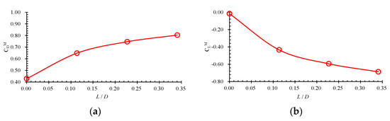
Figure 5.
Mean hydrodynamic coefficients of the pipeline: (a) mean drag coefficient, (b) mean lift coefficient.
It can be seen from Figure 5a that the mean drag coefficient on the pipeline increases with the increase of the spoiler length. In addition, it seems that the effect of the spoiler length on the mean drag coefficients becomes weak with the increasing spoiler length, reflecting by the decreasing slope of line as shown in Figure 5a. However, an opposite trend is observed for the mean lift coefficient. With an increasing spoiler length, the lift coefficient decreases accordingly, as shown in Figure 5b.
Figure 6 gives the variations of the mean hydrodynamic coefficients (represented by CDSM for the drag coefficient and CLSM for the lift coefficient, respectively) on the spoiler versus the spoiler length. It should be mentioned here that the spoiler length is used to define the Reynolds number when calculating the time-dependent hydrodynamic coefficients on the spoiler. It can be seen from Figure 6a that the mean drag coefficient on the spoiler increases with the increase of the spoiler length. Similar to the results shown in Figure 5a, the effect of the spoiler length on the mean drag coefficients of the spoiler becomes weak with the increasing spoiler length. However, the mean lift coefficient is found to increase with the increasing spoiler length and attains its maximum value at approximately L/D = 0.11. After that, the lift coefficient decreases with the further increase of the spoiler length.
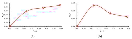
Figure 6.
Mean hydrodynamic coefficients of the spoiler: (a) mean drag coefficient, (b) mean lift coefficient.
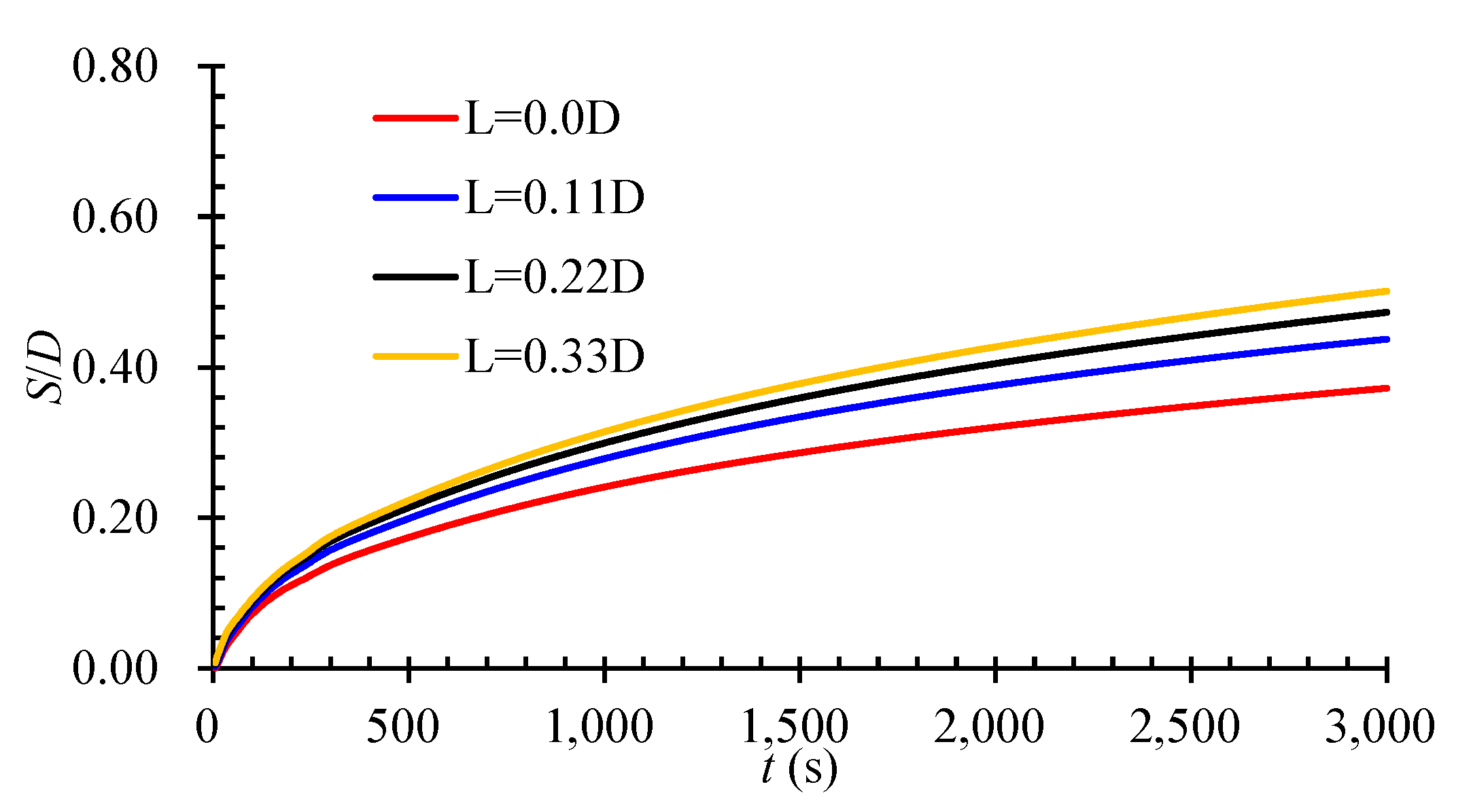
Figure 7 gives the time history of the scour depth beneath the pipeline with different spoiler lengths. It can be seen that the scour depth beneath the pipeline increases very fast when the time t < 500 s. After that, the scour depth increases with a lower speed. It is also found that the spoiler with a longer length leads to a deeper scour hole at the same time instant. For the pipeline without a spoiler, the scour depth beneath the pipeline at t = 3000 s is about 0.44 D, while for the pipeline with a spoiler length L = 0.33 D, the scour depth at t = 3000 s is approximately 0.57 D. The scour depth increases about 30% at t = 3000 s when the spoiler length increases from 0.0 D to 0.33 D.
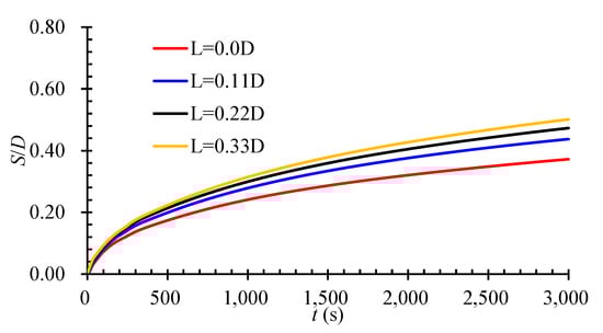
Figure 7.
Time history of scour depth beneath the pipeline.
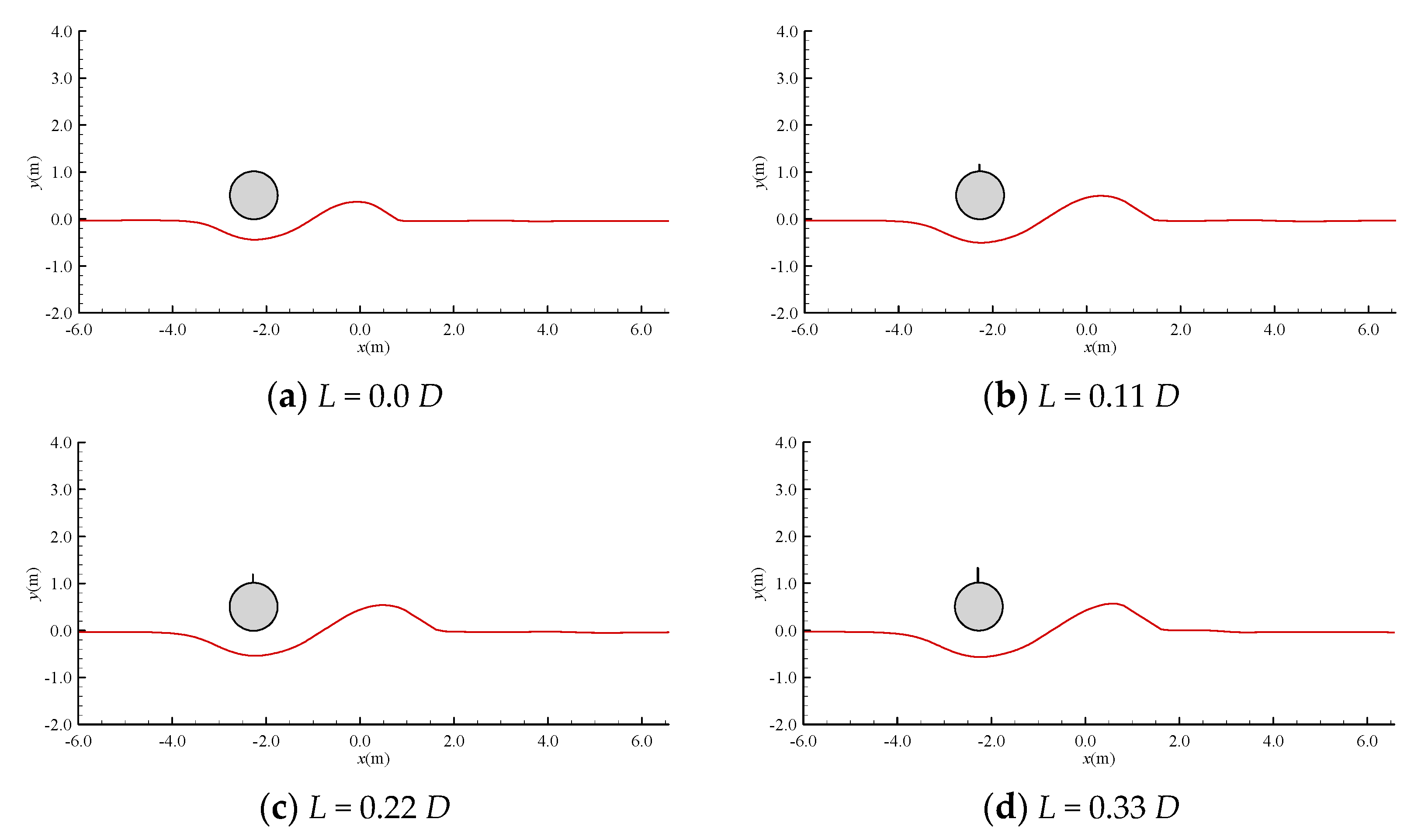
Figure 8 shows the numerical results of the local scour profile around the pipeline without and with a spoiler at t = 3000 s. It can be seen that although the scour profile does not change much for a pipeline with and without a spoiler, the scour range and the scour depth increase with the increase of the spoiler length.
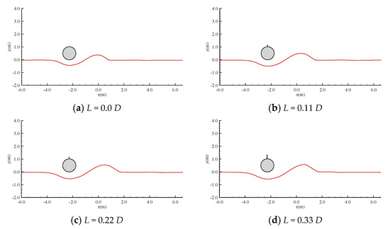
Figure 8.
The local scour profile around the pipeline without and with a spoiler at t = 3000 s.
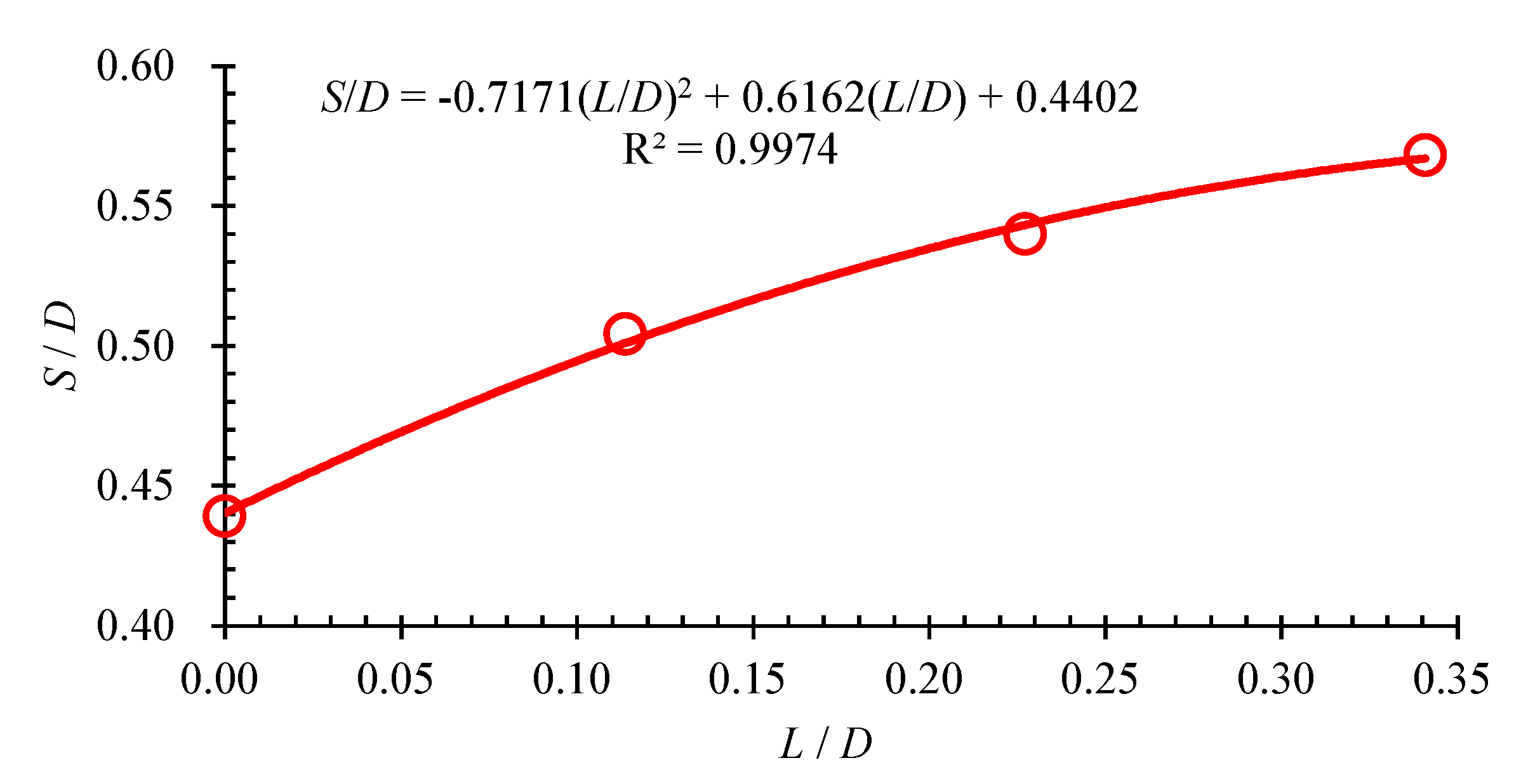
From the above discussion, it confirms that the spoiler length has a significant effect on the scour depth. To identify the detailed relationship, Figure 9 shows the dependence of the non-dimensional scour depth (S/D) on the non-dimensional spoiler length (L/D). The corresponding results shown in Figure 9 confirm again that a spoiler with a larger length leads to a deeper scour depth beneath the pipeline. This observation is consistent with the results given by Lee et al. [18], who found that a longer spoiler leads to a deeper scour depth with L/D = 0, 0.3 and 0.5, respectively. Based on the present numerical results, a quadratic polynomial function relationship is found between the scour depth and the spoiler length as follows:
S/D = −0.7171(L/D)2 + 0.6162(L/D) + 0.4402
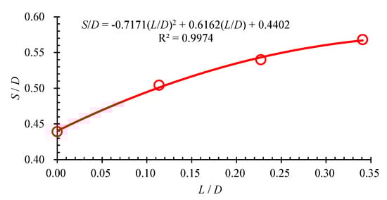
Figure 9.
Dependence of the scour depth beneath the pipeline on the spoiler length.
Further examination shows that the correlation coefficient is R2 = 0.9974, demonstrating that the scour depth is highly correlating to the spoiler length.
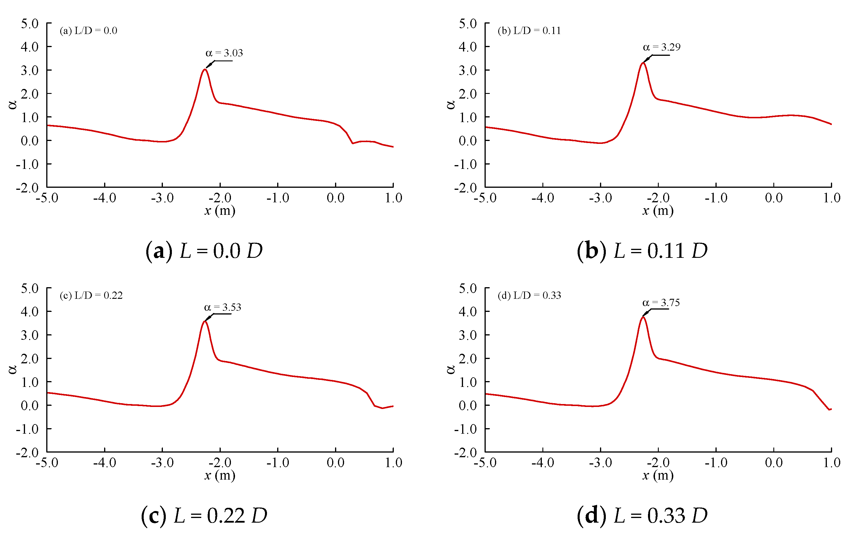
For further understanding the effect of the spoiler on the local scour around the submarine pipeline, Figure 10 presents the numerical results with respect to the distribution of the maximum amplification factor of the bed shear stress under different spoiler lengths. The amplification factor of the bed shear stress is defined as α = τ/τ0 with τ being the bed shear stress around the submarine pipeline and τ0 being the bed shear stress for the undisturbed flow. In the present study, the bed shear stress was calculated according to Equation (16). The horizontal velocity corresponding to the first layer of mesh nodes located at a distance Δ1 away from the seabed can be obtained, then the friction velocity uτ and the bed shear stress τ = ρuτ2 can also be determined.
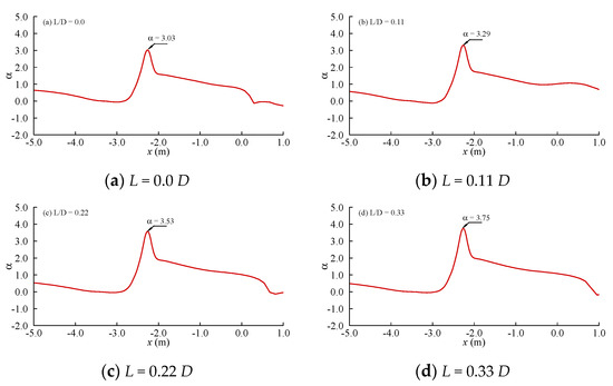
Figure 10.
The distribution of the maximum amplification factor of the bed shear stress under different spoiler lengths.
In the present study, the maximum amplification factor of the bed shear stress is presented, because the vertical scour rate is highly dependent on this variable [27]. It can be seen from Figure 10 that the profiles of the amplification factor α are very similar for different spoiler lengths. For α beneath the submarine pipeline, it is clearly shown that a longer spoiler leads to a larger α. The amplification factor α associated with L/D = 0.33 is 23.8% larger than that corresponding to L/D = 0.0. As reported by [27], the vertical scour rate (represented by ξ) of a submarine pipeline can be estimated by the relationship ξ ∞ A(ατ0-τcr)B, where A and B are two positive constant parameters and τcr is the critical shear stress. The above-mentioned parameters/variables can be obtained through apparent erosion rate measurements [28]. This relationship demonstrates that a larger bed shear stress will lead to a larger vertical scour rate ξ. This claim can be confirmed by the results shown in Figure 7. In Figure 7, it is found that the scour rate (reflected by the slopes of the lines) increases with the increase of the spoiler length. It has been known that the scour depth of a submarine pipeline is determined by both the vertical scour rate ξ and the time scale T*. As for the non-dimensional time scale, an empirical formula T* = 0.02θ−3/5 was proposed by [29] for both the steady currents and waves. The corresponding empirical formula suggests that T* is only governed by the incoming flow conditions. Based on the above analysis, it is concluded that the scour depth of the submarine pipeline with a spoiler is mainly controlled by the vertical scour rate ξ. The results shown in Figure 10 demonstrate that the pipeline with a longer spoiler corresponds to a faster vertical scour rate ξ, this results in a deeper scour depth as shown in Figure 9.
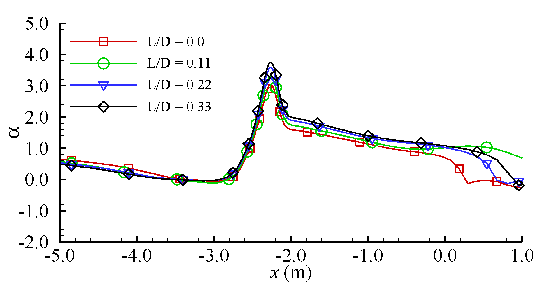
For a clear comparison, Figure 11 combines the plots shown in Figure 10 into one. Figure 12 presents the results of the maximum amplification factor of the bed shear stress α beneath the pipeline with respect to L/D.
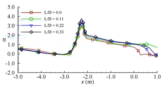
Figure 11.
The maximum amplification factor of the bed shear stress.
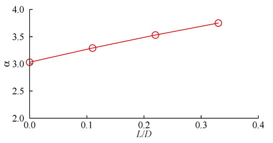
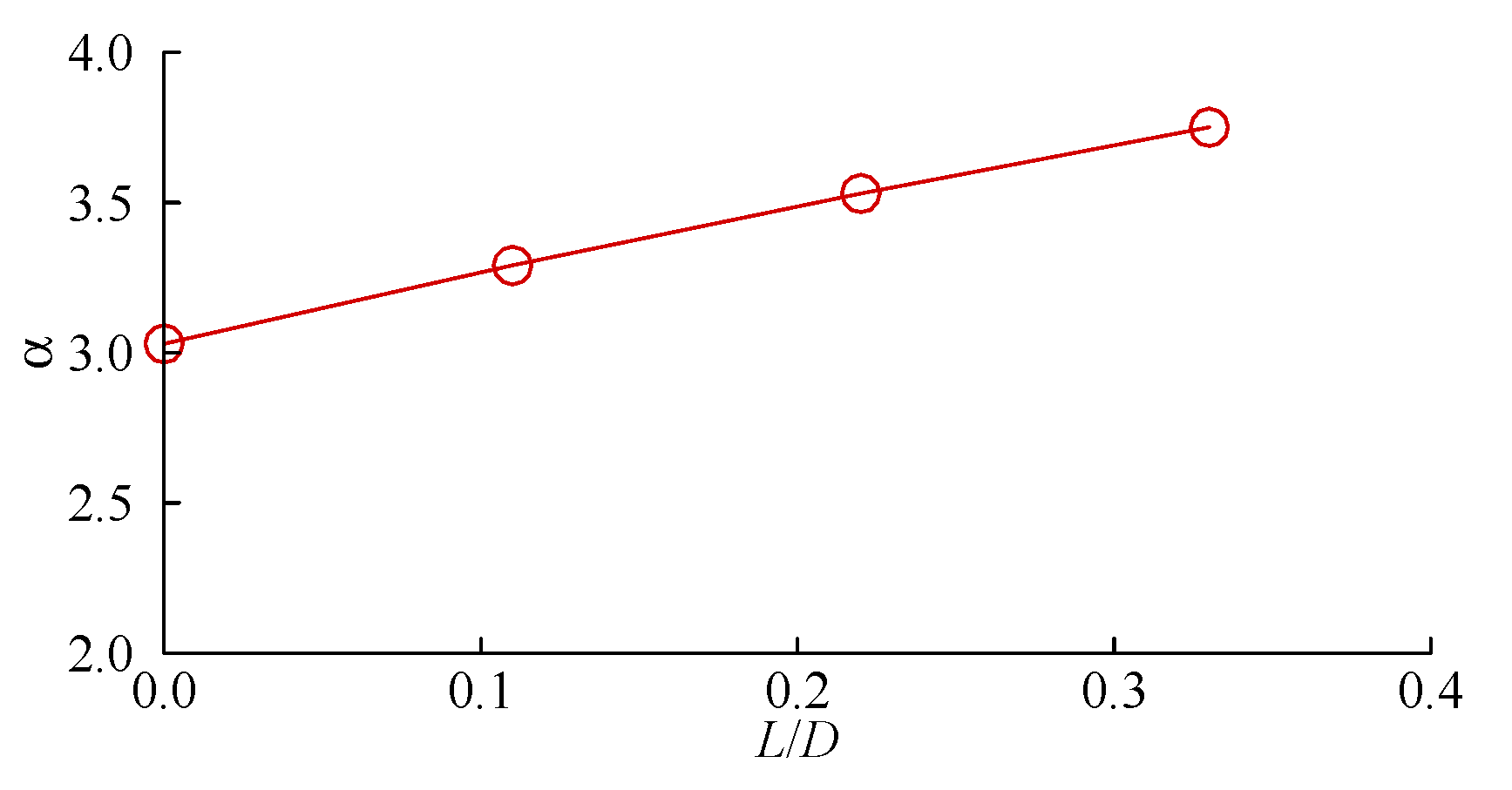
Figure 12.
The maximum amplification factor of the bed shear stress versus L/D.
It is found from Figure 12 that the maximum amplification factor of the bed shear stress α almost monotonously increases with the increase of the spoiler length.
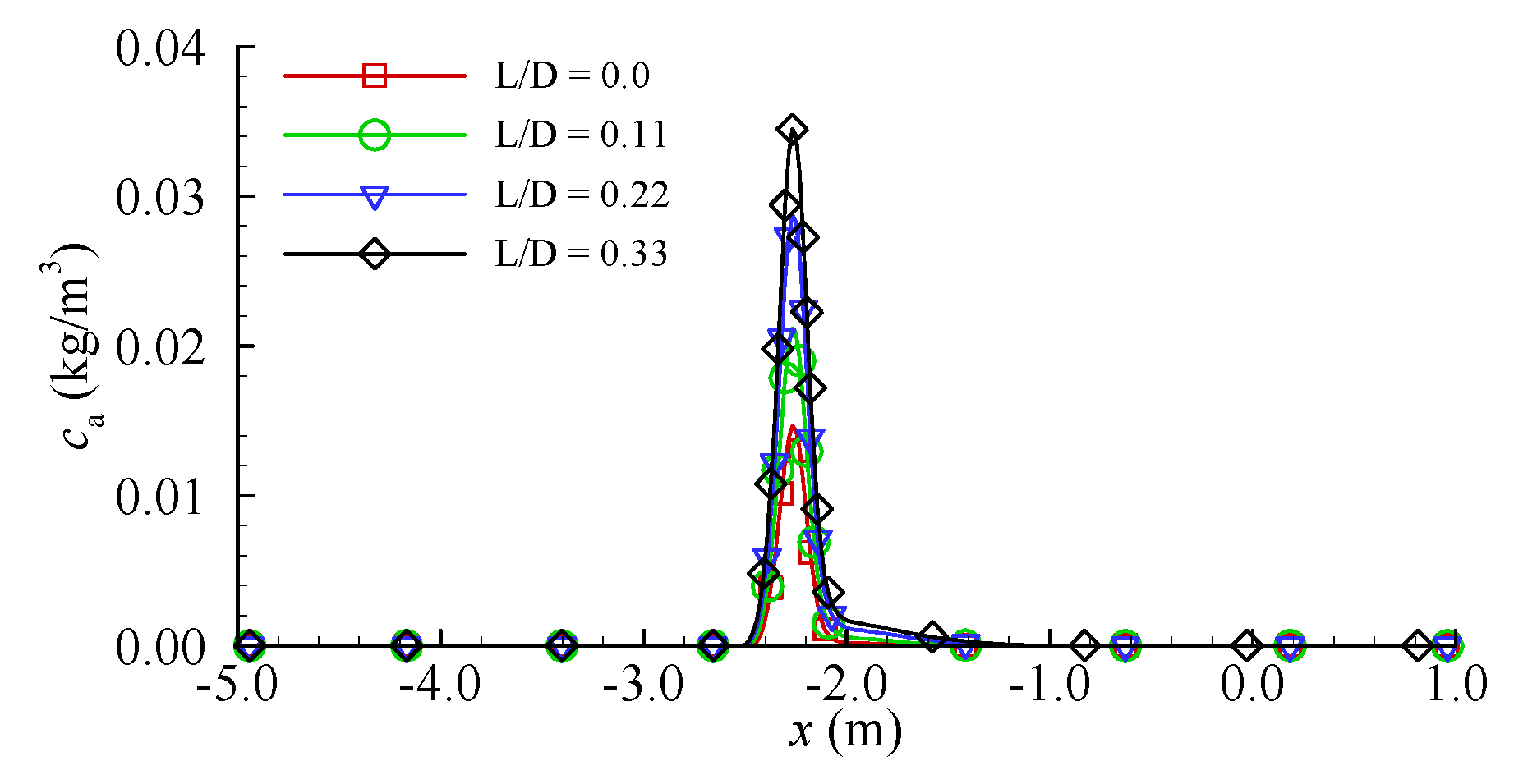
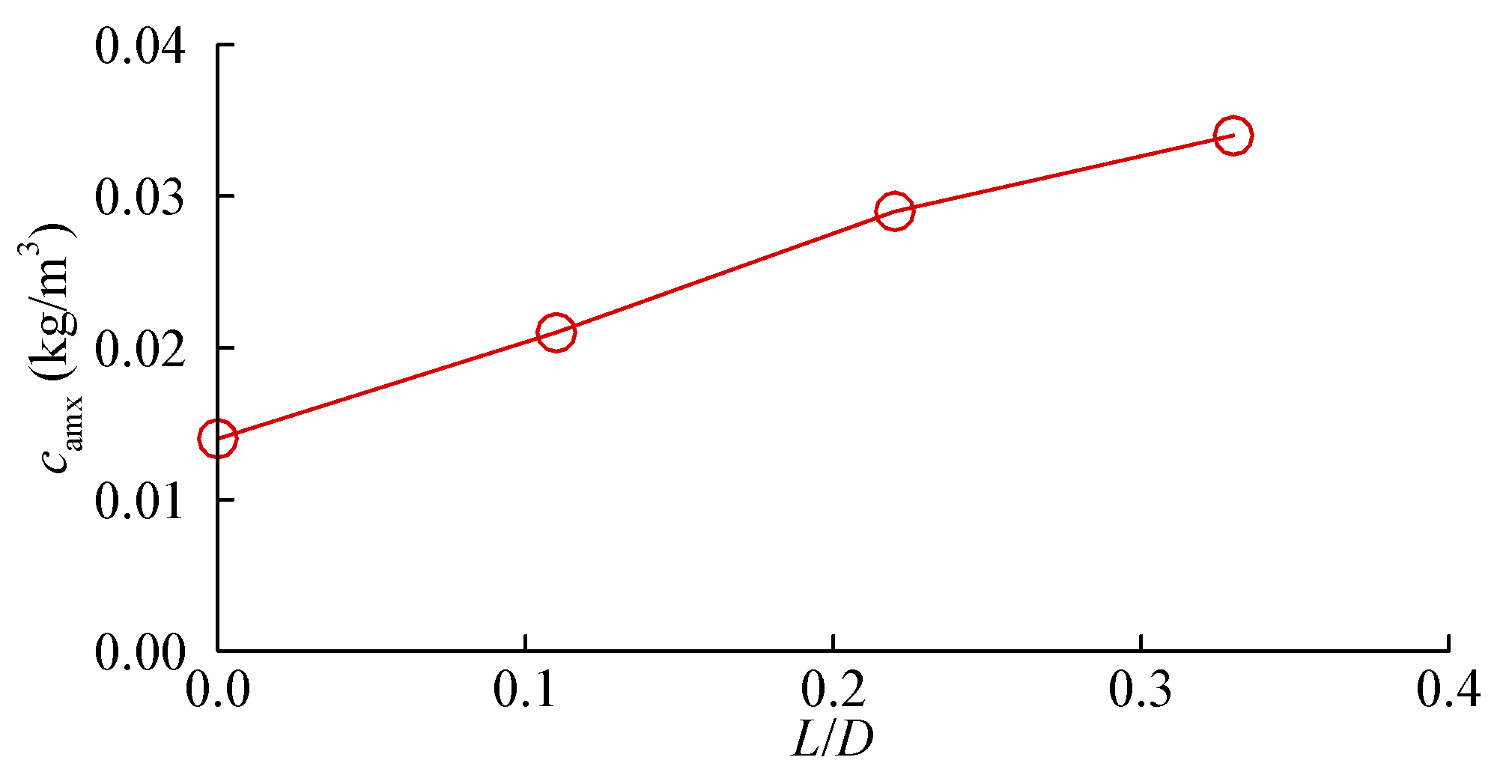
The concentration of the sediment particles is another factor affecting the scour depth. Figure 13 presents the numerical results the sediment concentration at a height 2.0d50 above the seabed based on Equation (18), these results are obtained at the time instant when the amplification factor of the bed shear stress achieves its maximum. Figure 14 gives the dependence of the maximum sediment concentration beneath the pipeline on the spoiler length.
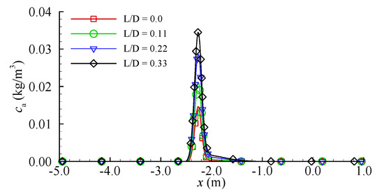
Figure 13.
The distribution of the sediment concentration under different spoiler lengths.

Figure 14.
The relationship between the sediment concentration beneath the submarine pipeline and the spoiler length.
It is observed from Figure 13 that the maximum sediment concentration occurs beneath the pipeline, and the pipeline with a longer spoiler is associated with a larger value of the sediment concentration. It is believed that this will result in a larger suspended load transport rate and the resultant deeper scour depth as shown in Figure 9. As for the distribution of the sediment concentration away from the pipeline, the corresponding values are approximately zero, because the Shields parameter θ is smaller than 0.045 at this time according to Equation (18). Similar to the results shown in Figure 12, the results shown in Figure 14 demonstrate that the maximum sediment concentration beneath the pipeline increases linearly with the increase of the spoiler length.
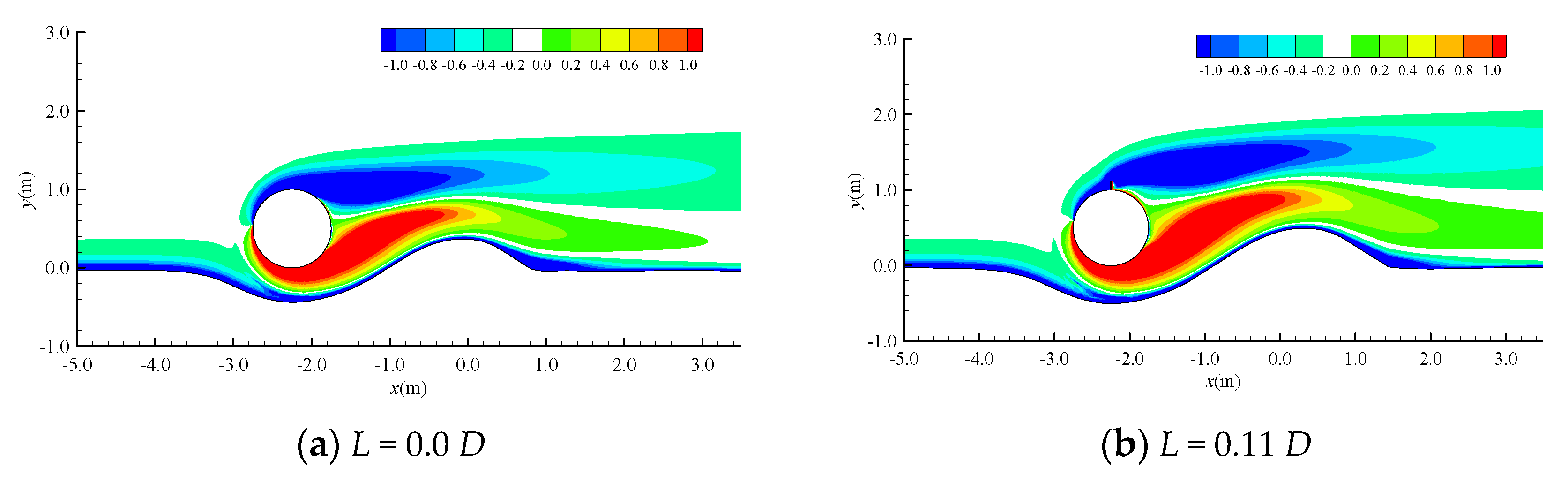
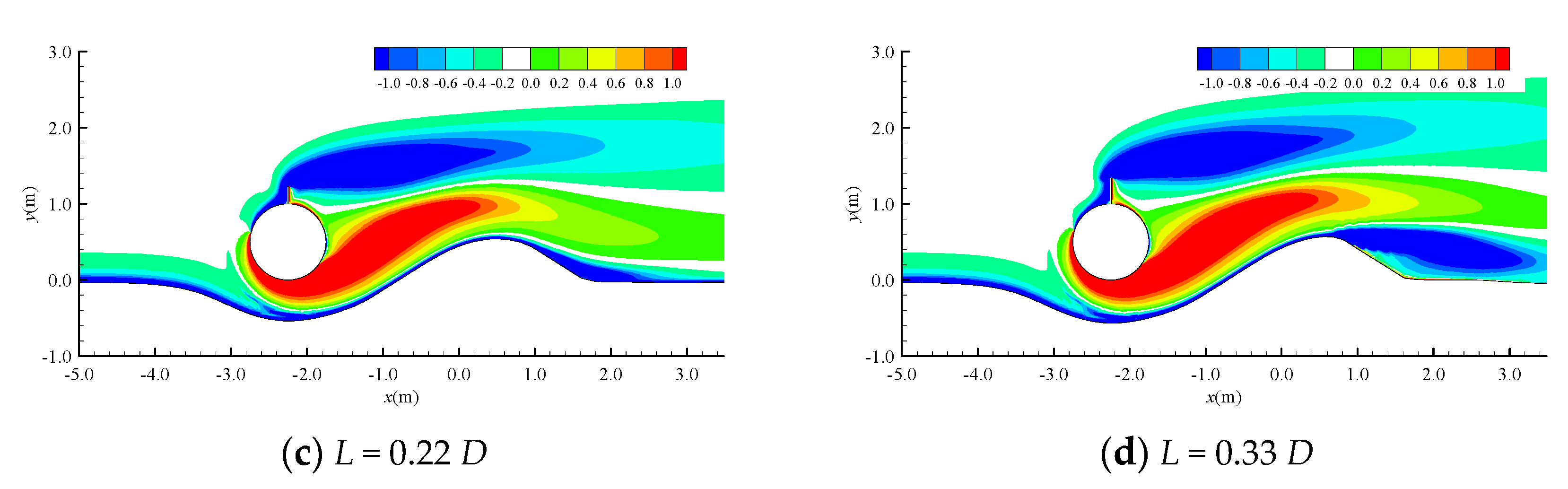
It is believed that the distribution of the vorticity (defined as ω’ = ∂v/∂x - ∂u/∂y, with its unit being 1/s) plays an important role in the local scour around the submarine pipeline. To support the above claim, Figure 15 shows the contour of the vorticity around the pipeline at t = 3000 s. It can be seen that the distributions of the vorticity are very similar for L = 0.0 D, 0.11 D, 0.22 D, 0.33 D, and this results in similar scour profiles around the pipeline. However, the length of the vortices behind the pipeline increases with the increasing spoiler length. The longer vortices cover a wider range of the seabed, and then impose a stronger shear effect on the seabed. This results in a larger scour range for the case with a larger spoiler length as shown in Figure 8.
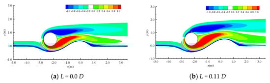

Figure 15.
Contour of the vorticity around the pipeline, the unit for the vorticity is 1/s.
4. Conclusions
A two-dimensional numerical model was developed to investigate the local scour around a submarine pipeline with a spoiler. The model is validated by comparing with the benchmarking published experimental data. In this study, the effects of the spoiler length on the scour depth, the time history of the local scour beneath the pipeline, the scour profile and the hydrodynamic coefficients on the pipeline were investigated using the validated model. Based on the numerical results, the main conclusions are summarized as follows:
- (1)
- The mean drag coefficients of the submarine pipeline and the spoiler increase with the increase of the spoiler length. It is also observed that the effect of the spoiler length on the mean drag coefficients becomes less pronounced with the increasing spoiler length for both the pipeline and the spoiler.
- (2)
- The mean lift coefficient of the pipeline decreases with the increasing spoiler length, while those on the spoiler show a different trend; the mean lift coefficients first increase with the increasing spoiler length and then decrease with its further increase. The maximum lift coefficient of the spoiler occurs at approximately L/D = 0.11.
- (3)
- The length of the spoiler has an important effect on the scour depth. The corresponding numerical results show that an increasing spoiler length generally leads to a deeper scour depth and a wider scour range. The scour depth with L/D = 0.33 is approximately 30% larger than that with L/D = 0. Further examination shows that the vortex behind a submarine pipeline with a longer spoiler becomes more longer, illustrated by the vorticity. The elongated vortex has a stronger interaction with the seabed, resulting in a deeper scour depth and a wider scour range.
- (4)
- The submarine pipeline with a longer spoiler corresponds to a larger amplification factor of the bed shear stress and a larger value of the sediment concentration beneath the pipeline, which contribute to the deeper scour depth.
Author Contributions
Conceptualization, C.Z. and J.L.; methodology, G.T.; software, G.T.; validation, J.W.; formal analysis, C.Z., J.L. and J.W.; investigation, G.T.; resources, J.W.; data curation, J.L.; writing—original draft preparation, J.W.; writing—review and editing, C.Z., J.L. and G.T.; visualization, G.T.; supervision, J.L.; project administration, C.Z.; funding acquisition, J.L. All authors have read and agreed to the published version of the manuscript.
Funding
This research was funded by the Science and Technology Project of ENERGY CHINA with grant number: GSKJ2-W01-2019.
Institutional Review Board Statement
Not applicable.
Informed Consent Statement
Informed consent was obtained from all subjects involved in the study.
Data Availability Statement
Not applicable.
Conflicts of Interest
The authors declare no conflict of interest.
Abbreviations
| ANSYS | Large general finite element analysis software |
| ALE | Arbitrary Lagrangian–Eulerian |
| RANS | Reynolds-averaged Navier–Stokes |
| SST | Shear Stress Transport |
| SUPG-FEM | The Streamline Upwind Petrov–Galerkin Finite Element Method |
| c | The concentration of the sediment |
| Cu | An empirical coefficient with its value being 0.09 |
| Ca | The boundary condition for the sediment concentration |
| CDM | The mean drag force coefficient |
| CLM | The mean lift force coefficient |
| CD(t) | The time-dependent drag coefficient |
| CL(t) | The time-dependent lift coefficient |
| CDSM | Mean drag coefficient |
| CLSM | Mean lift coefficient |
| d | Water depth |
| d50 | The median particle size of the sediment |
| D | Diameter of the submarine pipeline |
| D* | Dimensionless sediment grain size |
| FD(t) | The total drag forces |
| FL(t) | The total lift forces |
| k | The turbulence kinetic energy |
| KC | Keulegan–Carpenter number |
| L | The length of the spoiler |
| m | Constant parameter for calculating settling velocity of sediment |
| n | The unit outward normal vector |
| p | Pressure |
| qb | The bed load transport rate |
| qs | The suspended load transport rate |
| Re | The Reynolds number |
| R2 | The correlation coefficient |
| s | The ratio of the sediment density ρs to the fluid density ρ |
| S | The scour depth |
| Sij | The mean strain rate tensor |
| t | Time |
| T | Period of the wave motion |
| T0 | The parameter for estimating the bed load transport rate |
| T* | Time scale for local scour |
| uτ | The friction velocity |
| ui | Velocity component |
| ujm | The velocity of the moving grids |
| U | The amplitude of wave velocity |
| Ū | Deep averaged flow velocity |
| Uav | The magnitude of the fluid velocity |
| wsj | The settling velocity of sediment particle |
| ws0 | The settling velocity of sediment considering concentration |
| ya | Height above seabed |
| yb | The bottom bed elevation |
| ys | The height of the water free surface |
| Δ | The distance of the first layer meshes adjacent to the pipeline to the pipeline surface |
| Δ1 | Distance between the first layer mesh nodes and the seabed |
| Δt | The time period |
| Δb | The bed roughness |
| xi | Coordinates |
| α | Amplification factor of the bed shear stress |
| ρ | Fluid density |
| υ | The fluid kinematic viscosity coefficient |
| ξ | the vertical scour rate of a submarine pipeline |
| υt | The turbulent eddy viscosity |
| ω | Specific dissipation rate of the turbulence kinetic energy |
| ω′ | Vorticity |
| α | The local topographic slope of a seabed |
| δij | The Kronecker operator |
| κ | The Karman constant |
| λs | The porosity of the sediment |
| σc | The Schmidt number of the turbulence |
| τ | The bed shear stress |
| τcr | The critical shear stress |
| τ0 | The bed shear stress for the undisturbed flow |
| χ | The spatial averaged flow velocity |
| ψ | The sediment rest angle |
| θ | The Shields parameter |
| θ0 | the angle in the counterclockwise direction |
| θcr | The critical Shields parameter considering the local seabed slope |
| θcr0 | The critical Shields parameter |
References
- Breusers, H.N.C. Local Scour Near Offshore Structures; Delft Hydraulics Laboratory: Delft, The Netherlands, 1972; Publication No. 105. [Google Scholar]
- Kjeldsen, S.P.; Gjorsvik, C.; Bringaker, K.G.; Jacobsen, J. Local scour near offshore pipelines. In Proceedings of the Second International Conference on Port and Ocean Engineering Under Arctic Conditions (POAC), Reykjavik, Iceland, 27–30 August 1973; pp. 308–331. [Google Scholar]
- Bijker, E.W.; Leeuwestein, W. Interaction between pipelines and the seabed under the influence of waves and currents. In Seabed Mechanics; Denness, B., Ed.; Springer Science and Business M edia LLC: Dordrecht, The Netherlands, 1984; pp. 235–242. [Google Scholar]
- Ibrahim, A.; Nalluri, C. Scour prediction around marine pipelines. In Proceedings of the 5th International Symposium on Offshore Mechanics and Arctic Engineering, Tokyo, Japan, 13–18 April 1986; pp. 679–684. [Google Scholar]
- Sumer, B.M.; Fredsøe, J. The mechanics of Scour in the Marine Environment; World Scientific: Singapore, 2002. [Google Scholar]
- Hansen, E.A.; Fredsøe, J.; Mao, Y. Two dimensional scour below pipelines. In Proceedings of the 5th International Symposium on Offshore Mechanics and Arctic Engineering, Tokyo, Japan, 13–18 April 1986; pp. 670–678. [Google Scholar]
- Li, F.J.; Cheng, L. Numerical model for local scour under offshore pipelines. J. Hydraul. Eng. 1999, 125, 400–406. [Google Scholar] [CrossRef]
- Li, F.J.; Cheng, L. Prediction of lee-wake scouring of pipelines in currents. J. Waterw. Port Coast. Ocean Eng. 2001, 127, 106–112. [Google Scholar] [CrossRef]
- Li, F.J.; Cheng, L. Modelling of local scour below a sagging pipeline. Coast. Eng. 2003, 45, 189–210. [Google Scholar]
- Liu, M.M.; Jin, X.; Wang, L.; Yang, F.; Tang, J.B. Numerical investigation of local scour around a vibrating pipeline under steady currents. Ocean Eng. 2021, 221, 108546. [Google Scholar] [CrossRef]
- Zhao, M.; Cheng, L. Numerical investigation of local scour below a vibrating pipeline under steady currents. Coast. Eng. 2010, 57, 397–406. [Google Scholar] [CrossRef]
- Liang, D.F.; Cheng, L. Numerical model for wave-induced scour below a submarine pipeline. J. Waterw. Port Coast. Ocean Eng. 2005, 131, 193–202. [Google Scholar] [CrossRef]
- Sumer, B.M.; Fredsøe, J. Scour below pipelines in waves. J. Waterw. Port Coast. Ocean Eng. 1990, 116, 307–323. [Google Scholar] [CrossRef]
- Liu, M.M.; Lu, L.; Teng, B.; Zhao, M.; Tang, G.Q. Numerical modeling of local scour and forces for submarine pipeline under surface waves. Coast. Eng. 2016, 116, 275–288. [Google Scholar] [CrossRef]
- Liu, M.M. Numerical investigation of local scour around submerged pipeline in shoaling conditions. Ocean Eng. 2021, 234, 109258. [Google Scholar] [CrossRef]
- Öner, A.A. Numerical investigation of flow around a pipeline with a spoiler near a rigid bed. Adv. Mech. Eng. 2016, 8, 1–13. [Google Scholar] [CrossRef] [Green Version]
- Yang, L.P.; Shi, B.; Guo, Y.K.; Wen, X.Y. Calculation and experiment on scour depth for submarine pipeline with a spoiler. Ocean Eng. 2012, 55, 191–198. [Google Scholar] [CrossRef]
- Lee, W.D.; Jo, H.J.; Kim, H.S.; Kang, M.J.; Jung, K.H.; Hur, D.S. Experimental and numerical investigation of self-burial mechanism of pipeline with spoiler under steady flow conditions. J. Mar. Sci. Eng. 2019, 7, 456. [Google Scholar] [CrossRef] [Green Version]
- Menter, F.R. Two-equation eddy-viscosity turbulence models for engineering applications. AIAA J. 1994, 32, 1598–1605. [Google Scholar] [CrossRef] [Green Version]
- Menter, F.R.; Kuntz, M.; Langtry, R. Ten years of industrial experience with the SST turbulence model. Turbul. Heat Mass Transf. 2003, 4, 625–632. [Google Scholar]
- Richardson, J.F.; Zaki, W.N. Sedimentation and fluidization: Part I. Trans. Inst. Chem. Eng. 1954, 32, 35–53. [Google Scholar]
- Soulsby, R. Dynamics of Marine Sands; Tomas Telford: London, UK, 1997. [Google Scholar]
- Van Rijn, L.C. Mathematical Modeling of Morphological Processes in the Case of Suspended Sediment Transport. Ph.D. Thesis, Delft University of Technology, Delft, The Netherlands, 1978. [Google Scholar]
- Soulsby, R.; Whitehouse, R. Threshold of sediment motion in coastal environments. In Proceedings of the Combined Australasian Coastal Engineering and Ports Conference, Christchurch, New Zealand; 1997; pp. 149–154. Available online: https://search.informit.org/doi/abs/10.3316/INFORMIT.929741720399033 (accessed on 1 September 2021).
- Zhao, M.; Cheng, L.; Teng, B.; Dong, G.H. Hydrodynamic forces on dual cylinders of different diameters in steady currents. J. Fluids Struct. 2007, 23, 59–83. [Google Scholar] [CrossRef]
- Tang, G.Q.; Chen, C.Q.; Zhao, M.; Lu, L. Numerical simulation of flow past twin near-wall circular cylinders in tandem arrangement at low Reynolds number. Water Sci. Eng. 2015, 8, 315–325. [Google Scholar] [CrossRef] [Green Version]
- Draper, S.; Yao, W.D.; Cheng, L.; Tom, J.; An, H.W. Estimating the rate of scour propagation along a submarine pipeline in time-varying currents and in fine grained sediment. In Proceedings of the ASME 2018 37th International Conference on Ocean, Offshore and Arctic Engineering, Madrid, Spain, 17–22 June 2018. [Google Scholar]
- Mohr, M.; Draper, S.; Cheng, L.; White, D.J. Predicting the rate of scour beneath subsea pipelines in marine sediments under steady flow conditions. Coast. Eng. 2016, 110, 111–126. [Google Scholar] [CrossRef]
- Fredsøe, J.; Sumer, B.M.; Arnskov, M. Time scale for wave/current scour below pipelines. Int. J. Offshore Polar Eng. 1992, 2, 13–17. [Google Scholar]


Publisher’s Note: MDPI stays neutral with regard to jurisdictional claims in published maps and institutional affiliations. |
© 2021 by the authors. Licensee MDPI, Basel, Switzerland. This article is an open access article distributed under the terms and conditions of the Creative Commons Attribution (CC BY) license (https://creativecommons.org/licenses/by/4.0/).