A New Model for Determining the EOQ under Changing Price Parameters and Reordering Time

Abstract

The present study deals with the modification of Wilson’s formulation by taking into account changes in the supply chain represented by the parameters of the model, namely varying delivery costs and price of goods stored. The four different models are presented. The proposed models avoid the main drawbacks of Wilson’s formulation—the constant price and reordering time—and discuss the case where varying parameters are used alongside discounting. The proposed models render lower costs under particular settings.

1. Introduction

Sustainable business decisions require taking into account a wide range of factors and methodologies [1,2,3,4]. Therefore, a number of models have been proposed for efficient inventory management. In 1913, Harris introduced an economic order quantity concept to solve this problem in the form of a static formula (and started static inventory management models vein).

However, typical static economic order quantity (EOQ) models [5,6] do not satisfy practitioners because of their incapacity to consider changing consumer demand, requiring constant orders in equal periods of time [7]. Unpredictable and constantly changing demands, affecting the size and frequency of orders, lead to situations in which classical inventory management models become unfit for solving practical inventory management problems and motivate a search for new or modified alternatives. In the last decade, we observed increased scientific interest in solving this problem. Firstly, Sana [8] proposed an EOQ model for perishable goods reacting to retail price changes, although practical implementation is restricted by neglecting the minimizing effect of a negative power function of price, which generates high sensibility in consumer’s demand. Later, Dobson et al. [9] proposed that perishable goods, with the demand rate as a linearly decreasing function of the age of the products, act similarly to nonperishable goods with the unit holding cost equal to the ratio of contribution margin to lifetime. In their model, they obtain traditional nonperishable Economic Order Quantity (EOQ)-like lower and upper bounds on the cycle length and the profit and show that they lead to near-optimal results for typical examples, like grocery items. Zeng et al. [10] formulate an extension to Wilson’s model varying quantity of order and different ordering periods. Their model generates a substantial economic effect when a significant change in consumer demand is noticed and (or) a long period of planning the logistics process must be ensured.

Conventional models for inventory management with uncertain demand, such as variations of Harris formulation [11,12,13], Markov equation-based ones [14,15], and Wilson’s formulation [16,17,18,19] are designed to minimize the expected costs of replenishment and stock-outs. They assume that complete satisfaction of uncertain and hardly predictable demand is too expensive or even deemed impossible. All these models are designed under the constant order quantity principle, where the size of the following order is based on the objective to minimize the whole cost of a company’s inventory management.

The problem of economic order quantity (EOQ) is quite well-known and has been widely discussed in the scientific literature [20,21,22,23,24]. Determination of the EOQ has a particular importance in trade and retail activities. The optimal ordering plan allows for the companies to achieve smooth operation and competitive advantage [25,26,27].

In the context of steady economic growth, the EOQ models assuming steady demand for perishable consumer goods are suitable for determining the lot size [28,29,30]. There has been research on the EOQ with respect to the credit market [31] and stock dynamic sizing optimization under the Logistic 4.0 environment for material management of a very high-speed train [32].

However, the fluctuations in the demand and lead time have not been taken into account. Indeed, such fluctuations become more important during disruptions of the supply chains (e.g., due to pandemic events). The emergence of trade barriers requires retailers to reconsider the optimal lot size. This issue is further aggravated by fluctuations in the market prices of particular products. Indeed, the crisis affects the consumer behavior and demand for particular goods [33,34,35]. The changes in demand are reflected by the prices of the products retailed [36,37]. Therefore, one needs to adjust decisions to order and store goods. Even without facing serious crisis, changes in pricing occur over time in terms of both retail market and storage costs. Thus, a mathematical model capable of determining the optimal economic order quantity under varying reordering time and price parameters is obvious. Although there has been a wide range of models proposed for determining the lot sizes (Table 1), none of them are able to handle the varying stock quantity based on varying price and reordering time.

Table 1. Overview of the existing economic order quantity (EOQ) models.

No.	Reference	Model
1.	Sebatjane & Adetunji [38].	Costs per cycle are multiplied by the number of cycles. Discounting is not applied.
2.	Khan, Jaber & Bonney, M. [39]	Optimal order quantity in the presence of defective items in the order and with various options for defect detection: no implications to changing price parameters of an order are provided.
3.	Birbil, Ş. İ., Bülbül, K., Frenk, H., & Mulder, H. M. [40]	The demand and unit price are assumed to be constant.
4.	Taleizadeh, A. A. [41]	Divided payments are considered assuming constant parameters of the model.
5.	Molamohamadi, Z., Arshizadeh, R., Ismail, N., & Azizi, A. [42]	The delay of payment is allowed (it may be considered as a proxy for changing price parameters of the order). The objective is optimizing trade credit terms rather than the lot size.
6.	El-Kassar, A. N., Salameh, M., & Bitar, M. [43]	The model allows for identifying faulty intermediate consumption items rather than determining the optimal lot size.
7.	Tungalag, N., Erdenebat, M., & Enkhbat, R. [44]	EOQ extended with the Euler–Lagrange equation without varying price parameters.
8.	Jaggi, C. K., & Mittal, M. [45]	EOQ model with a focus on the lot size with regards to defected items and deterioration time.
9.	Elyasi, M., Khoshalhan, F., & Khanmirzaee, M. [46]	The EOQ model with constant price and lead time.
10.	Widyadana, G. A., Cárdenas-Barrón, L. E., & Wee, H. M. [47]	The model for deteriorating items.
11.	Shanshan, L. & Yong, H. [1]	Focus on mitigating effects of an already occurred stock out.
12.	Inprasit, T. & Tanachutiwat, S. [48]	A combination of machine learning and neural networks for determining a reordering point but not an EOQ.

This paper presents a model for determining the optimal lot size with fluctuating price building on the classical Wilson’s formulation following extensions by Slesarenko and Nestorenko [49] and by Zeng et al. [10]. The proposed model optimizes the discounted costs of all orders rather than the costs per order. Due to this fundamental difference, our model is more relevant to economic decision making and ensures symmetry in the decision process. Presenting practical application of models with different parameters, we also show how this model performs in real-life situations.

2. The Proposed Model of Lot Management with Time-Variant Cost Parameters

Inventory management is understood as the definition of optimal controllable parameters (time between deliveries $t_s$ (time set up) and q (quantity, or optimal order size)) of logistics processes, at which the minimum total costs (TC) for the purchase, delivery, and storage of goods is achieved for a certain planned time interval [0, T]. If the uncontrollable parameters of the logistics process (purchase price p, delivery cost $c_s$, (cost set up) daily demand μ, and daily interest rate i (r = i/100%) are known and constant throughout the entire planning interval, this problem can be solved by using Wilson economic-mathematical model EOQ (Economic Order Quantity):

$$TC\left(t_s\right)=pD+\frac{c_{s}T}{t_s}+\frac{1}{2}{c}_{h}D{t}_s$$

(1)

where D is the demand for the period (time interval) $\left[0,T\right]$ ($D=\mu T$) and $c_h$ is the cost of storing a unit of goods per day (holding cost).

The optimal time between deliveries $\left(t_{so}\right)$ and optimal order quantity ($q_o$) are found according to the Wilson formula:

$$t_{so}=t_w=\sqrt{\frac{2c_{s}T}{c_{h}D}}$$

(2)

$$q_o=\mu t_{so}$$

(3)

Slesarenko and Nestorenko [49], and Nestorenko et al. [50] proposed the modified EOQ model:

$$TC\left(t_s\right)=\left(c_s+p\mu t_s\right)\frac{{\left(1+r\right)}^{t_s}\left({\left(1+r\right)}^T-1\right)}{{\left(1+r\right)}^{t_s}-1}$$

(4)

The optimal time between deliveries is found by the following formula:

$$t_{so}=\sqrt{\frac{2c_s}{rp\mu }}$$

(5)

The formula coincides with Wilson’s Formula (2) if the storage cost is expressed as a percentage of the unit price ($c_h=p\mu$).

If the parameters of the logistic process change, the optimal solution is recalculated using Wilson’s Formula (5), taking into account the changes. Based on the available information, it is possible to build forecasts for further economic processes of behavior. The use of this information in economic and mathematical models leads to an increase in their adequacy and accuracy.

Zeng et al. [10] proposed models of inventory management that allow for determining the optimal values of parameters in the case when it is known that daily demand has a linear trend ($\mu \left(t\right)=\mu +\omega t,t\in \left[0,T\right]$). To find those parameters, it is necessary to use Wilson’s Formula (5), replacing the constant value of daily demand μ with the arithmetic mean of daily demand $\overline{\mu }$ for the planning period $\left[0,T\right]$ ($\overline{\mu }=\mu +0.5\omega T$).

We further construct economic and mathematical models of inventory management that allow for determining the values of optimal controlled parameters in the case when it is known that uncontrolled cost parameters (delivery cost and/or price) have uniform relative trends ($c_s\left(t\right)=c_s{\left(1+{\rho }_c\right)}^t,p\left(t\right)=p{\left(1+{\rho }_p\right)}^t,t\in \left[0,T\right]$).

Model 1.

The inventory management model with a simultaneous equal percentage change in the costs of delivery and prices (inflationary model).

In the EOQ model, the uncontrollable cost parameters as the cost of delivery ($c_s=const$) and price ($p=const)$ for the period [0, T] will be replaced by the assumption that the cost of delivery and the price simultaneously change uniformly with equal percentage change ($c_s\left(t\right)=c_s{\left(1+\rho \right)}^t,p\left(t\right)=p{\left(1+\rho \right)}^t,t\in \left[0,T\right]$). It is an inflationary process when ρ > 0 and a deflationary one when ρ < 0.

The logistics process of purchasing, delivering, and storing goods with constant time between deliveries can be described by the following formula:

$$\begin{gathered} TC\left(t_s\right)=\left(c_s+p\mu t_s\right){\left(1+r\right)}^{n{t}_s}+\left(c_s{\left(1+\rho \right)}^{t_s}+p{\left(1+\rho \right)}^{t_s}\mu t_s\right){\left(1+r\right)}^{\left(n-1\right)t_s}+\cdots \\ +\left(c_s{\left(1+\rho \right)}^{\left(n-1\right)t_s}+p{\left(1+\rho \right)}^{\left(n-1\right)t_s}\mu t_s\right){\left(1+r\right)}^{t_s} \end{gathered}$$

(6)

where $n$ is the number of deliveries of consignments of goods for the period $\left[0,T\right]$ ($n=T/t_s$). Replacing it, we get the following:

$${\left(1+r\right)}^{j{t}_s}=e^{\ln \left(1+r\right)j{t}_s},{\left(1+\rho \right)}^{j{t}_s}=e^{\ln \left(1+\rho \right)j{t}_s},j=\overline{1,n}$$

After performing arithmetic transformations, we get the following:

$$TC\left(t_s\right)=\left(c_s+p\mu t_s\right)e^{\ln \left(1+r\right)T}\left(1+e^{(\ln \left(1+\rho \right)-\ln \left(1+r\right))t_s}+\cdots +e^{\left(n-1\right)(\ln \left(1+\rho \right)-\ln \left(1+r\right))t_s}\right)$$

(7)

Using the formula for the sum of the first members of a geometric progression, we get the formula for total costs:

$$TC\left(t_s\right)=\left(c_s+p\mu t_s\right)\frac{(e^{\ln \left(1+r\right)-\ln \left(1+\rho \right))T}-1)e^{\ln \left(1+\rho \right)T}}{e^{(\ln \left(1+r\right)-\ln \left(1+\rho \right))t_s}-1}$$

(8)

The minimum total cost is obtained as follows:

$$\begin{array}{cc}\frac{dTC\left(t_s\right)}{d{t}_s}=\hfill & p\mu \frac{(e^{\left(\ln \left(1+r\right)-\ln \left(1+\rho \right)\right)T}-1)e^{\ln \left(1+\rho \right)T}}{e^{(\ln \left(1+r\right)-\ln \left(1+\rho \right))t_s}-1}-(\ln \left(1+r\right)\hfill \\ \hfill & -\ln \left(1+\rho \right))\left(c_s+p\mu t_s\right)\frac{e^{(\ln \left(1+r\right)-\ln \left(1+\rho \right))t_s}(e^{\left(\ln \left(1+r\right)-\ln \left(1+\rho \right)\right)T}-1)e^{\ln \left(1+\rho \right)T}}{{\left(e^{(\ln \left(1+r\right)-\ln \left(1+\rho \right))t_s}-1\right)}^2}\hfill \\ \hfill & =0\hfill \end{array}$$

(9)

After transformations, the equation is as follows:

$$e^{\left(\ln \left(1+r\right)-\ln \left(1+\rho \right)\right)t_s}-1=\left(\ln \left(1+r\right)-\ln \left(1+\rho \right)\right)\left(\frac{c_s}{p\mu }+t_s\right)$$

(10)

The optimal time between deliveries of consignments of goods $t_{so}$ is found from solving the nonlinear Equation (10). In order to find an approximate solution to Equation (10), we use the first three terms of the Maclaurin series [51] of the expansion of the function $y=e^x\approx 1+x+0.5x^2$ and the first term of the Maclaurin series of the expansion of the function $y=\ln \left(1+r\right)\approx r$.

$$t_{so}=t_s=\sqrt{\frac{2c_s}{\left(\mathrm{r}-\rho \right)p\mu }}$$

(11)

Therefore, to determine the optimal time between deliveries of consignments of goods $t_{so}$, one can use Wilson’s Formula (5), replacing r with the difference r − ρ.

Let $\alpha =\ln \left(1+\rho \right)/\ln \left(1+r\right)\approx \rho /r$. Then, Equation (11) can be written as follows:

$$t_{so}=\frac{t_w}{\sqrt{1-\alpha }}$$

(12)

The dependence of the optimal time between deliveries of consignments of goods $t_{so}$ on α is shown in Figure 1. When $\alpha \ge {\alpha }_{max}=1-\frac{t_w^2}{T^2}$, it is necessary to purchase in the volume $q_o=\mu T$ and to deliver the goods once for the entire planning period of the logistic process. When $\alpha \le {\alpha }_{min}=1-t_w^2$, it is necessary to purchase and deliver goods every day in the amount of $q_o=\mu$. When ${\alpha }_{min}<\alpha <{\alpha }_{max}$, it is necessary to purchase and deliver goods in $t_{so}=\frac{t_w}{\sqrt{1-\alpha }}$ days and in volume $q_o=\frac{\mu t_w}{\sqrt{1-\alpha }}=\frac{q_w}{\sqrt{1-\alpha }}$.

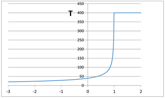
Figure 1. Dependence of the optimal time between deliveries of consignments of goods $t_{so}$ on α.

Change in the dependence of total costs $TC\left(t_s,\alpha \right)$ on the time between deliveries of consignments of goods $t_s$ for different values of α as well as the dependence of the minimum total costs $TC\left(t_{so},\alpha \right)$ on the optimal time between deliveries of consignments of goods $t_{so}$ for different values of α (black line and black squares) are shown in Figure 2.

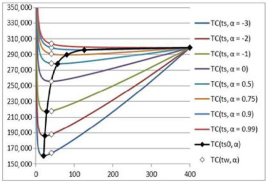
Figure 2. Dependence of total costs $TC\left(t_s,\alpha \right)$ on the time between deliveries of consignments of goods $t_s$ for different α values; dependence of the minimum total costs $TC\left(t_{so},\alpha \right)$ on the optimal time between deliveries of consignments of goods $t_{so}$ for different values α; and the value of the total costs $TC\left(t_w,\alpha \right)$ for the time between deliveries of the consignment $t_w$ for different α values.

Note: If we determine the values of the controlled parameters at i moment ($i=1,2,3\dots )$ of decision-making according to Wilson’s Formula (5), we get the same time between deliveries equal to $t_w$:

$$t_{si}=\sqrt{\frac{2c_s{\left(1+\rho \right)}^{t_{si}}}{rp{\left(1+\rho \right)}^{t_{si}}\mu }}=\sqrt{\frac{2c_s}{rp\mu }}=t_w,i=1,2,3\dots$$

(13)

This option on making decision is not optimal (differs from (11)). The result of using this option for different values of α (white squares) is also shown in Figure 2

Model 2.

The inventory management model with the percentage change in the cost of delivery.

In the EOQ model, the assumption about constancy of the uncontrolled parameter delivery cost ($c_s=const$) for the period $\left[0,T\right]$ is replaced by the assumption in which the delivery cost changes uniformly according to the regularity $c_s\left(t\right)=c_s{\left(1+{\rho }_c\right)}^t,t\in \left[0,T\right]$. If ${\rho }_c>0$, there is an increase in the cost of delivery; if ${\rho }_c<0$, there is a decrease.

Then, the logistics process of purchasing, delivering, and storing goods with constant time between deliveries can be described by the following formula:

$$\begin{gathered} TC\left(t_s\right)=\left(c_s+p\mu t_s\right){\left(1+r\right)}^{n{t}_s}+\left(c_s{\left(1+{\rho }_c\right)}^{t_s}+p\mu t_s\right){\left(1+r\right)}^{\left(n-1\right)t_s}+\cdots \\ +\left(c_s{\left(1+{\rho }_c\right)}^{\left(n-1\right)t_s}+p\mu t_s\right){\left(1+r\right)}^{t_s} \end{gathered}$$

(14)

where n is the number of deliveries of consignments of goods for the period $\left[0,T\right]$ ($n=T/t_s$).

Replacing it, we get the following:

$${\left(1+r\right)}^{j{t}_s}=e^{\ln \left(1+r\right)j{t}_s},{\left(1+{\rho }_c\right)}^{j{t}_s}=e^{\ln \left(1+{\rho }_c\right)j{t}_s},j=\overline{1,n}$$

After performing arithmetic transformations, we get the following:

$$\begin{gathered} TC\left(t_s\right)=e^{\ln \left(1+r\right)T}\left(c_s\left(1+e^{(\ln \left(1+{\rho }_c\right)-\ln \left(1+r\right))t_s}+\cdots +e^{\left(n-1\right)(\ln \left(1+{\rho }_c\right)-\ln \left(1+r\right))t_s}\right) \\ +p\mu t_s\left(1+e^{-\ln \left(1+r\right)t_s}+\cdots +e^{-\ln \left(1+r\right)\left(n-1\right)t_s}\right)\right) \end{gathered}$$

(15)

Using the formula for the sum of the first members of a geometric progression, we get the formula for total costs:

$$TC\left(t_s\right)=c_s\frac{e^{(\ln \left(1+r\right)-\ln \left(1+{\rho }_c\right))t_s}\left(e^{\ln \left(1+r\right)T}-e^{\ln \left(1+{\rho }_c\right)T}\right)}{e^{(\ln \left(1+r\right)-\ln \left(1+{\rho }_c\right))t_s}-1}+p\mu t_s\frac{e^{\ln \left(1+r\right)t_s}\left(e^{\ln \left(1+r\right)T}-1\right)}{e^{\ln \left(1+r\right)t_s}-1}$$

(16)

The minimum total costs is as follows:

$$\begin{array}{c}\frac{dTC\left(t_s\right)}{d{t}_s}\hfill \\ =p\mu \frac{e^{\ln \left(1+r\right)t_s}\left(e^{\ln \left(1+r\right)T}-1\right)}{e^{\ln \left(1+r\right)t_s}-1}-\ln \left(1+r\right)p\mu t_s\frac{e^{\ln \left(1+r\right))t_s}\left(e^{\ln \left(1+r\right)T}-1\right)}{{\left(e^{\ln \left(1+r\right)t_s}-1\right)}^2}\hfill \\ -c_s\frac{(\ln \left(1+r\right)-\ln \left(1+{\rho }_c\right))e^{(\ln \left(1+r\right)-\ln \left(1+{\rho }_c\right))t_s}\left(e^{\ln \left(1+r\right)T}-e^{\ln \left(1+{\rho }_c\right)T}\right)}{{\left(e^{(\ln \left(1+r\right)-\ln \left(1+{\rho }_c\right))t_s}-1\right)}^2}=0\hfill \end{array}$$

(17)

After transformations, the equation is as follows:

$$\begin{array}{c}{e}^{\ln \left(1+r\right)t_s}-1-\ln \left(1+r\right)t_s\hfill \\ =\frac{c_s}{p\mu }\frac{(\ln \left(1+r\right)-\ln \left(1+{\rho }_c\right)){\left(e^{\ln \left(1+r\right)t_s}-1\right)}^2}{e^{\ln \left(1+{\rho }_c\right)}{\left(e^{(\ln \left(1+r\right)-\ln \left(1+{\rho }_c\right))t_s}-1\right)}^2}\frac{\left(e^{\ln \left(1+r\right)T}-e^{\ln \left(1+{\rho }_c\right)T}\right)}{\left(e^{\ln \left(1+r\right)T}-1\right)}\hfill \end{array}$$

(18)

In model 2, the optimal time between deliveries of consignments of goods $t_{so}$ is also found from the solution of the nonlinear Equation (18). In order to find an approximate solution of Equation (18), we use the first three terms of the Maclaurin series of the expansion of the function $y=e^x\approx 1+x+0.5x^2$ and the first term of the Maclaurin series of the expansion of the function $y=\ln \left(1+r\right)\approx r$.

$$t_{so}=t_s=\sqrt{\frac{2c_s{\left(1+{\rho }_c\right)}^{\frac{1}{2}T}}{\mathrm{r}p\mu }}$$

(19)

Consequently, to determine the optimal time between deliveries of consignments of goods $t_{so}$, one can use Wilson’s Formula (5), replacing the constant value of the delivery cost $c_s$ with the geometric mean of the delivery cost $\overline{c_s}$ for the planning period $\left[0,T\right]$ ($\overline{c_s}=\sqrt{c_s{c}_s{\left(1+{\rho }_c\right)}^T}=c_s{\left(1+{\rho }_c\right)}^{\frac{1}{2}T}$).

$$t_{so}={\left(1+{\rho }_c\right)}^{\frac{1}{4}T}{t}_w$$

(20)

Let ${\alpha }_c=\ln \left(1+{\rho }_c\right)/\ln \left(1+r\right)$; then Equation (20) can be represented in this form:

$$t_{so}={\left(1+r\right)}^{\frac{1}{4}{\alpha }_{c}T}{t}_w$$

(21)

The dependence of the optimal time between deliveries of consignments of goods $t_{so}$ on ${\alpha }_c$ is shown in Figure 3.

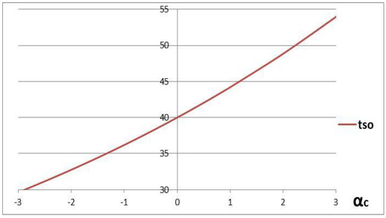
Figure 3. The dependence of optimal time between deliveries of consignments of goods $t_{so}$ on ${\alpha }_c$.

The change in the dependence of total costs $TC\left(t_s,{\alpha }_c\right)$ on the time between deliveries of consignments of goods $t_s$ for different ${\alpha }_c$ values as well as the dependence of the minimum total costs $TC\left(t_{so},{\alpha }_c\right)$ on the optimal time between deliveries of consignments of goods $t_{so}$ for different ${\alpha }_c$ values (black line and black squares) are shown in Figure 4.

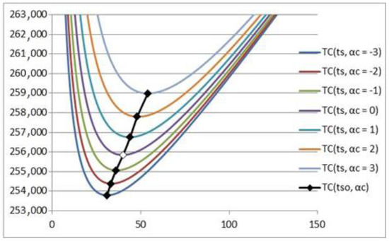
Figure 4. The dependence of total costs $TC\left(t_s,{\alpha }_c\right)$ on the time between deliveries of consignments of goods $t_s$ for different ${\alpha }_c$ values and the dependence of the minimum total costs $TC\left(t_{so},{\alpha }_c\right)$ on the optimal time between deliveries of consignments of goods $t_{so}$ for different ${\alpha }_c$ values (black line and black squares).

Model 3.

Inventory management model with a percentage change in the price of goods.

In the EOQ model, the assumption of the constancy of the uncontrollable parameter of the product price ($p=const$) for the period $\left[0,T\right]$ is replaced by the assumption that the price of the product changes uniformly according to the order that $p\left(t\right)=c_p{\left(1+{\rho }_p\right)}^t,t\in \left[0,T\right]$). If ${\rho }_p>0$, there is an increase in the price of goods, and if ${\rho }_p<0$, there is a decrease.

To construct model 3, we will use the results from constructing model 1 (8) and model 2 (16). We represent the change (increase/decrease) in the price as a combination of two processes—the change (increase/decrease) in the price and delivery cost (model 1) and the simultaneous change (decrease/increase) in the delivery cost (model 2) by the same number of times. A change in the price and delivery cost, according to model 1, will lead to the replacement of $\ln \left(1+r\right)$ to $\ln \left(1+r\right)-\ln \left(1+{\rho }_p\right)$ in Formula (16) and will be multiplied by $e^{\ln \left(1+{\rho }_p\right)T}$. To compensate for the change in the cost of delivery, according to model 2, we make a replacement $1+{\rho }_c=1/(1+{\rho }_p)$:

$$\begin{array}{cc}\hfill TC\left(t_s\right)=& c_s\frac{e^{\ln \left(1+r\right)t_s}\left(e^{\ln \left(1+r\right)T}-1\right)}{e^{\ln \left(1+r\right)t_s}-1}\hfill \\ \hfill & +p\mu t_s\frac{e^{(\ln \left(1+r\right)-\ln \left(1+{\rho }_p\right))t_s}\left(e^{(\ln \left(1+r\right)-\ln \left(1+{\rho }_p\right))T}-1\right)e^{\ln \left(1+{\rho }_p\right)T}}{e^{(\ln \left(1+r\right)-\ln \left(1+{\rho }_p\right))t_s}-1}\hfill \end{array}$$

(22)

The minimum total cost is found as follows:

$$\begin{array}{c}\frac{dTC\left(t_s\right)}{d{t}_s}\hfill \\ =-c_s\frac{\ln \left(1+r\right)e^{\ln \left(1+r\right)t_s}\left(e^{\ln \left(1+r\right)T}-1\right)}{{\left(e^{\ln \left(1+r\right)t_s}-1\right)}^2}\hfill \\ +p\mu \frac{e^{(\ln \left(1+r\right)-\ln \left(1+{\rho }_p\right))t_s}\left(e^{(\ln \left(1+r\right)-\ln \left(1+{\rho }_p\right))T}-1\right)e^{\ln \left(1+{\rho }_p\right)T}}{e^{(\ln \left(1+r\right)-\ln \left(1+{\rho }_p\right))t_s}-1}\hfill \\ -p\mu t_s\frac{(\ln \left(1+r\right)-\ln \left(1+{\rho }_p\right))e^{(\ln \left(1+r\right)-\ln \left(1+{\rho }_p\right))t_s}\left(e^{(\ln \left(1+r\right)-\ln \left(1+{\rho }_p\right))T}-1\right)e^{\ln \left(1+{\rho }_p\right)T}}{{\left(e^{(\ln \left(1+r\right)-\ln \left(1+{\rho }_p\right))t_s}-1\right)}^2}\hfill \\ =0\hfill \end{array}$$

(23)

After transformations, the equation is as follows:

$$\begin{array}{cc}\hfill e^{(\ln \left(1+r\right)-\ln \left(1+{\rho }_p\right))t_s}& -1-(\ln \left(1+r\right)-\ln \left(1+{\rho }_p\right))t_s\hfill \\ \hfill & =\frac{c_s}{p\mu }\frac{\ln \left(1+r\right)e^{\ln \left(1+{\rho }_p\right)t_s}{\left(e^{(\ln \left(1+r\right)-\ln \left(1+{\rho }_p\right))t_s}-1\right)}^2\left(e^{\ln \left(1+r\right)T}-1\right)}{{\left(e^{\ln \left(1+r\right)t_s}-1\right)}^2\left(e^{(\ln \left(1+r\right)-\ln \left(1+{\rho }_p\right))T}-1\right)e^{\ln \left(1+{\rho }_p\right)T}}\hfill \end{array}$$

(24)

We repeat the previously mentioned procedure: the optimal time between deliveries of consignments of goods $t_{so}$ is found from the solution of the nonlinear Equation (24). In order to find an approximate solution of Equation (24), we use the first three terms of the Maclaurin series of the expansion of the function $y=e^x\approx 1+x+0.5x^2$ and the first term of the Maclaurin series of the expansion of the function $y=\ln \left(1+r\right)\approx r$.

$$t_s=\sqrt{\frac{2c_s}{\left(r-{\rho }_p\right)p{e}^{\frac{1}{2}\ln \left(1+{\rho }_p\right)T}\mu }}$$

(25)

Consequently, to determine the optimal time between deliveries of consignments of goods $t_{so}$, one can use Wilson’s Formula (5), replacing r by the difference $r-\rho$ and the constant value of the price of goods $p$ with the geometric mean of the price of goods $\overline{p}$ for the planning period $\left[0,T\right]$ ($\overline{p}=\sqrt{pp{\left(1+{\rho }_p\right)}^T}=p{\left(1+{\rho }_p\right)}^{\frac{1}{2}T}$).

Let ${\alpha }_p=\ln \left(1+{\rho }_p\right)/\ln \left(1+r\right)$; then Equation (25) can be represented as follows:

$$t_{so}=\frac{t_w}{{\left(1+{\rho }_p\right)}^{\frac{1}{4}T}\sqrt{1-{\alpha }_p}}$$

(26)

or

$$t_{so}=\frac{t_w}{{\left(1+r\right)}^{\frac{1}{4}{\alpha }_{p}T}\sqrt{1-{\alpha }_p}}$$

(27)

The dependence of the optimal time between deliveries of consignments of goods $t_{so}$ on ${\alpha }_c$ is shown in Figure 5.

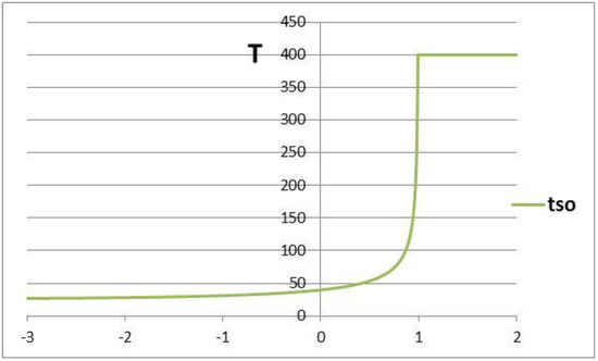
Figure 5. The dependence of the optimal time between deliveries of consignments of goods $t_{so}$ on ${\alpha }_c$.

The change in the dependence of total costs $TC\left(t_s,{\alpha }_p\right)$ on the time between deliveries of consignments of goods $t_s$ for different ${\alpha }_p$ values as well as the dependence of the minimum total costs $TC\left(t_{so},{\alpha }_p\right)$ on the optimal time between deliveries of consignments of goods $t_{so}$ for different ${\alpha }_p$ values (black line and black squares) are shown in Figure 6.

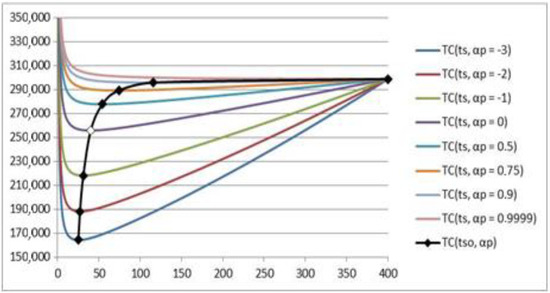
Figure 6. The dependence of total costs $TC\left(t_s,{\alpha }_p\right)$ on the time between deliveries of consignments of goods $t_s$ for different ${\alpha }_p$ values and the dependence of the minimum total costs $TC\left(t_{so},{\alpha }_p\right)$ on the optimal time between deliveries of consignments of goods $t_{so}$ for different ${\alpha }_p$ values (black line and black squares).

Model 4.

Inventory management model with a different percentage change in the price of goods.

In the EOQ model, the assumption of the constancy of the uncontrollable parameter of the product price ($p=const$) for the period $\left[0,T\right]$ is replaced by the assumption that the price of the product changes uniformly according to the order that $p\left(t\right)=c_p{\left(1+{\rho }_p\right)}^t,t\in \left[0,T\right]$). If ${\rho }_p>0$, there is an increase in the price of goods, and if ${\rho }_p<0$, there is a decrease.

To construct model 4, we will use the results from constructing model 1 (8) and model 2 (16). We represent the change (increase/decrease) in the price as a combination of two processes—the change (increase/decrease) in the price and delivery cost (model 1) and the simultaneous change (decrease/increase) in the delivery cost by a certain number of times. A change in the price and delivery cost, according to model 1, will lead to the replacement of $\ln \left(1+r\right)$ to $\ln \left(1+r\right)-\ln \left(1+{\rho }_p\right)$ in Formula (16) and will be multiplied by $e^{\ln \left(1+{\rho }_p\right)T}$. The change in the cost of delivery, according to model 2, we will receive by replacement of $1+{\rho }_c=\left(1+{\rho }_c\right)/(1+{\rho }_p)$:

$$\begin{array}{cc}\hfill TC\left(t_s\right)=& c_s\frac{e^{\left(\ln \left(1+r\right)-\ln \left(1+{\rho }_c\right)\right)t_s}\left(e^{\left(\ln \left(1+r\right)-\ln \left(1+{\rho }_c\right)\right)T}-1\right)e^{\ln \left(1+{\rho }_c\right)T}}{e^{\left(\ln \left(1+r\right)-\ln \left(1+{\rho }_c\right)\right)t_s}-1}\hfill \\ \hfill & +p\mu t_s\frac{e^{\left(\ln \left(1+r\right)-\ln \left(1+{\rho }_p\right)\right)t_s}\left(e^{\left(\ln \left(1+r\right)-\ln \left(1+{\rho }_p\right)\right)T}-1\right)e^{\ln \left(1+{\rho }_p\right)T}}{e^{\left(\ln \left(1+r\right)-\ln \left(1+{\rho }_p\right)\right)t_s}-1}\hfill \end{array}$$

(28)

The minimum total costs are found as follows:

$$\begin{array}{c}\frac{dTC\left(t_s\right)}{d{t}_s}\hfill \\ =p\mu \frac{e^{\left(\ln \left(1+r\right)-\ln \left(1+{\rho }_p\right)\right)t_s}\left(e^{\left(\ln \left(1+r\right)-\ln \left(1+{\rho }_p\right)\right)T}-1\right)e^{\ln \left(1+{\rho }_p\right)T}}{e^{\left(\ln \left(1+r\right)-\ln \left(1+{\rho }_p\right)\right)t_s}-1}\hfill \\ -c_s\frac{\left(\ln \left(1+r\right)-\ln \left(1+{\rho }_c\right)\right)e^{\left(\ln \left(1+r\right)-\ln \left(1+{\rho }_c\right)\right)t_s}\left(e^{\left(\ln \left(1+r\right)-\ln \left(1+{\rho }_c\right)\right)T}-1\right)e^{\ln \left(1+{\rho }_c\right)T}}{{\left(e^{\left(\ln \left(1+r\right)-\ln \left(1+{\rho }_c\right)\right)t_s}-1\right)}^2}\hfill \\ p\mu t_s\frac{\left(\ln \left(1+r\right)-\ln \left(1+{\rho }_p\right)\right)e^{\left(\ln \left(1+r\right)-\ln \left(1+{\rho }_p\right)\right)t_s}\left(e^{\left(\ln \left(1+r\right)-\ln \left(1+{\rho }_p\right)\right)T}-1\right)e^{\ln \left(1+{\rho }_p\right)T}}{{\left(e^{\left(\ln \left(1+r\right)-\ln \left(1+{\rho }_p\right)\right)t_s}-1\right)}^2}=0\hfill \end{array}$$

(29)

After transformations, the equation appears as follows:

$$\begin{array}{c}{e}^{\left(\ln \left(1+r\right)-\ln \left(1+{\rho }_p\right)\right)t_s}-1-\left(\ln \left(1+r\right)-\ln \left(1+{\rho }_p\right)\right)t_s\hfill \\ =\frac{C_s}{p_{\mu }}\frac{(\ln \left(1+r\right)-\ln \left(1+{\rho }_c\right))e^{(\ln \left(1+{\rho }_p\right)-\ln \left(1+{\rho }_c\right))t_s}{\left(e^{(\ln \left(1+r\right)-\ln \left(1+{\rho }_p\right))t_s}-1\right)}^2(e^{\ln \left(1+r\right)T}-e^{\ln \left(1+{\rho }_c\right)T})}{{\left(e^{(\ln \left(1+r\right)-\ln \left(1+{\rho }_c\right))t_s}-1\right)}^2(e^{\ln \left(1+r\right)T}-e^{\ln \left({\rho }_p\right)T})}\hfill \end{array}$$

(30)

The optimal time between deliveries of consignments of goods $t_{so}$ is found from the solution of the nonlinear Equation (30). In order to find an approximate solution of Equation (30), we use the first three terms of the Maclaurin series of the expansion of the function $y=e^x\approx 1+x+0.5x^2$ and the first term of the Maclaurin series of the expansion of the function $y=\ln \left(1+r\right)\approx r$.

$$t_{so}=t_s=\sqrt{\frac{2c_s{\left(1+{\rho }_c\right)}^{\frac{1}{2}T}}{\left(\mathrm{r}-{\rho }_p\right)p{\left(1+{\rho }_p\right)}^{\frac{1}{2}T}\mu }}$$

(31)

Consequently, to determine the optimal time between deliveries of consignments of goods $t_{so}$, one can use Wilson’s Formula (5), replacing r by the difference $r-\rho$ and the constant value of the price of goods $p$ with the geometric mean of the price of goods $\overline{p}$ for the planning period $\left[0,T\right]$ ($\overline{p}=\sqrt{pp{\left(1+{\rho }_p\right)}^T}=p{\left(1+{\rho }_p\right)}^{\frac{1}{2}T}$) and the constant value of the product price $c_s$ by geometric mean value of the product price $\overline{c_s}$ for the planning period $\left[0,T\right]$ ($\overline{c_s}=\sqrt{c_s{c}_s{\left(1+{\rho }_c\right)}^T}=c_s{\left(1+{\rho }_c\right)}^{\frac{1}{2}T}$).

Let ${\alpha }_p=\ln \left(1+{\rho }_p\right)/\ln \left(1+r\right)\mathrm{and}{\alpha }_c=\ln \left(1+{\rho }_c\right)/\ln \left(1+r\right)$; then Equation (31) can be represented as follows:

$$t_{so}=\frac{{\left(1+{\rho }_c\right)}^{\frac{1}{4}T}}{{\left(1+{\rho }_p\right)}^{\frac{1}{4}T}}\frac{t_w}{\sqrt{1-{\alpha }_p}}$$

(32)

or

$$t_{so}={\left(1+r\right)}^{\frac{1}{4}\left({\alpha }_c-{\alpha }_p\right)T}\frac{t_w}{\sqrt{1-{\alpha }_p}}$$

(33)

The dependence of the optimal time between deliveries of consignments of goods $t_{so}$ on ${\alpha }_c$ and ${\alpha }_p$ is shown in Figure 7.

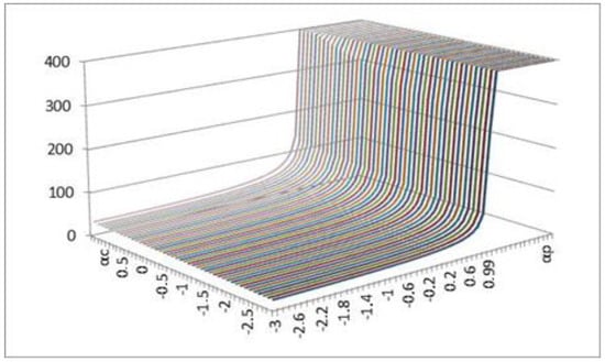
Figure 7. The dependence of the optimal time between deliveries of consignments of goods $t_{so}$ on ${\alpha }_c$ and ${\alpha }_p.$

The change in the dependence of the total costs $TC\left(t_s,{\alpha }_c=-3,{\alpha }_p\right)$ with a decrease in the cost of delivery (${\alpha }_c=-3$) on the time between deliveries of consignments of goods $t_s$ at different ${\alpha }_p$ values as well as the dependence of the minimum total costs $TC\left(t_{so},{\alpha }_c=-3,{\alpha }_p\right)$ on the optimal time between deliveries of consignments of goods $t_{so}$ for different ${\alpha }_p$ values (black line and black squares) are shown in Figure 8.

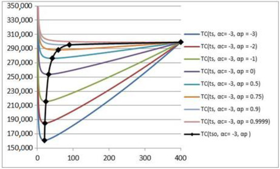
Figure 8. The dependence of the total costs $TC\left(t_s,{\alpha }_c=-3,{\alpha }_p\right)$ with a decrease in the cost of delivery (${\alpha }_c=-3$) on the time between deliveries of consignments of goods $t_s$ at different ${\alpha }_p$ values and the dependence of the minimum total costs $TC\left(t_{so},{\alpha }_c=-3,{\alpha }_p\right)$ on the optimal time between deliveries of consignments of goods $t_{so}$ for different ${\alpha }_p$ values (black line and black squares).

The change in the dependence of total costs $TC\left(t_s,{\alpha }_c=0,{\alpha }_p\right)$ at constant delivery cost (${\alpha }_c=0$) on the time between deliveries of consignments of goods $t_s$ for different ${\alpha }_p$ values as well as the dependence of the minimum total costs $TC\left(t_{so},{\alpha }_c=0,{\alpha }_p\right)$ on the optimal time between deliveries of consignments of goods $t_{so}$ for different ${\alpha }_p$ values (black line and black squares) are shown in Figure 6.

The change in the dependence of total costs $TC\left(t_s,{\alpha }_c=3,{\alpha }_p\right)$ with an increase in the cost of delivery (${\alpha }_c=3$) on the time between deliveries of consignments of goods $t_s$ for different ${\alpha }_p$ values as well as the dependence of the minimum total costs $TC\left(t_{so},{\alpha }_c=3,{\alpha }_p\right)$ on the optimal time between deliveries of consignments of goods $t_{so}$ for different ${\alpha }_p$ values (black line and black squares) are shown in Figure 9.

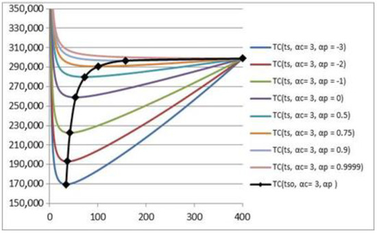
Figure 9. The dependence of total costs $TC\left(t_s,{\alpha }_c=3,{\alpha }_p\right)$ with an increase in the cost of delivery (${\alpha }_c=3$) on the time between deliveries of consignments of goods $t_s$ for different ${\alpha }_p$ values and the dependence of the minimum total costs $TC\left(t_{so},{\alpha }_c=3,{\alpha }_p\right)$ on the optimal time between deliveries of consignments of goods $t_{so}$ for different ${\alpha }_p$ values (black line and black squares).

Model 4 is a generalization of models 1–3:

• for ${\alpha }_c={\alpha }_p$ we obtain model 1;
• for ${\alpha }_p=0$ we obtain model 2; and
• for ${\alpha }_c=0$ we obtain model 3.

Further, we provide some examples of the differences that arise when using models 1–4 and the modified EOQ model.

3. Empirical illustration

Model 1

If at the beginning of the period [0, T], uncontrollable parameters of the logistic process such as T = 400 days, r = 0.001, and μ = 25 units/day are known and the cost of delivery and the price increases equally during the period [0, T] with ρ = 0.00075, then the growth pattern will be $c_s\left(t\right)=400\ast {1.00075}^t,p\left(t\right)=20\ast {1.00075}^t,t\in \left[0,T\right]$($\alpha =0.75$).

When using the EOQ model, excluding the increase in delivery costs and prices, the time between deliveries will be the following:

$$t_w=\sqrt{\frac{2\ast 400}{0.001\ast 20\ast 25}}=40\mathrm{days}$$

The total purchase, delivery, and storage costs for 400 days are as follows:

$$\begin{gathered} T{C}_w=\left(400+20\ast 25\ast 40\right)\ast {1.001}^{400}+\left(400\ast {1.00075}^{40}+20\ast {1.00075}^{40}\ast 25\ast 40\right)\ast {1.001}^{360}+\cdots +\left(400\ast {1.00075}^{360}+20\ast {1.00075}^{360}\ast 25\ast 40\right)\ast {1.001}^{40}= \\ 290911\mathrm{EUR} \end{gathered}$$

When applying model 1, the time between deliveries is found by Formula (12):

$$t_{so}=\frac{40}{\sqrt{1-0.75}}=80\mathrm{days}$$

The total purchase, delivery, and storage costs for 400 days are as follows:

$$\begin{gathered} T{C}_o=\left(400+20\ast 25\ast 80\right)\ast {1.001}^{400}+\left(400\ast {1.00075}^{80}+20\ast {1.00075}^{80}\ast 25\ast 80\right)\ast {1.001}^{320}+\cdots +\left(400\ast {1.00075}^{320}+20\ast {1.00075}^{320}\ast 25\ast 80\right)\ast {1.001}^{80}= \\ 289600\mathrm{EUR} \end{gathered}$$

The savings will be as follows:

$$\Delta TC=290911-289600=1311\mathrm{EUR}$$

If the cost of delivery and the price decrease equally during the period [0, T] with ρ = −0.003, the growth pattern has the following form: $c_s\left(t\right)=400\ast {0.997}^t,p\left(t\right)=20\ast {0.997}^t,t\in \left[0,T\right]$ ($\alpha =-3$).

When using the EOQ model, excluding the reduction in delivery costs and prices, the time between deliveries will be $t_w=40$ days.

The total purchase, delivery, and storage costs for 400 days are as follows:

$$T{C}_w=\left(400+20\ast 25\ast 40\right)\ast {1.001}^{400}+\left(400\ast {0.997}^{40}+20\ast {0.997}^{40}\ast 25\ast 40\right)\ast {1.001}^{360}+\cdots +\left(400\ast {0.997}^{360}+20\ast {0.997}^{360}\ast 25\ast 40\right)\ast {1.001}^{40}=164156\mathrm{EUR}$$

When applying model 1, the time between deliveries is found by Formula (12):

$$t_{so}=\frac{40}{\sqrt{1+3}}=20\mathrm{days}$$

The total purchase, delivery, and storage costs for 400 days are as follows:

$$\begin{gathered} T{C}_o=\left(400+20\ast 25\ast 20\right)\ast {1.001}^{400}+\left(400\ast {0.997}^{20}+20\ast {0.997}^{20}\ast 25\ast 20\right)\ast \\ {1.001}^{380}+\cdots +\left(400\ast {0.997}^{380}+20\ast {0.997}^{380}\ast 25\ast 20\right)\ast {1.001}^{20}=160934\mathrm{EUR} \end{gathered}$$

The savings will be as follows:

$$\Delta TC=164156-160934=3222\mathrm{EUR}$$

Model 2

If at the beginning of the period [0, T] uncontrollable parameters of the logistic process such as T = 400 days, r = 0.001, μ = 25 units/day, and $p=20$ EUR/unit are known and the cost of delivery increases during the period [0, T] with ρ = 0.00075, then the growth pattern will be $c_s\left(t\right)=400\ast {1.0023}^t,t\in \left[0,T\right]$ (${\alpha }_c=2.3$).

When using the EOQ model, excluding the increase in delivery costs, the time between deliveries will be $t_w=40$ days.

The total purchase, delivery, and storage costs for 400 days are as follows:

$$\begin{gathered} T{C}_w=\left(400+20\ast 25\ast 40\right)\ast {1.001}^{400}+\left(400\ast {1.0022}^{40}+20\ast 25\ast 40\right)\ast \\ {1.001}^{360}+\cdots +\left(400\ast {1.0022}^{360}+20\ast 25\ast 40\right)\ast {1.001}^{40}=258365\mathrm{EUR} \end{gathered}$$

When applying model 2, the time between deliveries is found by Formula (20):

$$t_{so}={1.0023}^{100}\ast 40=50\mathrm{days}$$

The total purchase, delivery, and storage costs for 400 days are as follows:

$$\begin{gathered} T{C}_o=\left(400+20\ast 25\ast 50\right)\ast {1.001}^{400}+\left(400\ast {1.0022}^{50}+20\ast 25\ast 50\right)\ast \\ {1.001}^{350}+\cdots +\left(400\ast {1.0022}^{320}+20\ast 25\ast 50\right)\ast {1.001}^{50}=258068\mathrm{EUR} \end{gathered}$$

The savings will be as follows:

$$\Delta TC=258365-258068=297\mathrm{EUR}$$

If the cost of delivery decreases during the period [0, T] with ${\rho }_c=-0.0018$, the growth pattern has the form $c_s\left(t\right)=400\ast {0.9982}^t,t\in \left[0,T\right]$ (${\alpha }_c=-1.8$).

When using the EOQ model, excluding delivery cost reduction, the time between deliveries will be $t_w=40$ days.

The total purchase, delivery, and storage costs for 400 days are as follows:

$$\begin{gathered} T{C}_w=\left(400+20\ast 25\ast 40\right)\ast {1.001}^{400}+\left(400\ast {0.9982}^{40}+20\ast 25\ast 40\right)\ast \\ {1.001}^{360}+\cdots +\left(400\ast {0.9982}^{360}+20\ast 25\ast 40\right)\ast {1.001}^{40}=254627\mathrm{EUR} \end{gathered}$$

When applying model 2, the time between deliveries is found by Formula (20):

$$t_{so}={0.9982}^{100}\ast 40=33\mathrm{days}$$

The total purchase, delivery, and storage costs for 400 days are as follows:

$$\begin{gathered} T{C}_o=\left(400+20\ast 25\ast 33\right)\ast {1.001}^{400}+\left(400\ast {0.9982}^{33}+20\ast 25\ast 33\right)\ast \\ {1.001}^{367}+\cdots +\left(400\ast {0.9982}^{367}+20\ast 25\ast 33\right)\ast {1.001}^{33}=254513\mathrm{EUR} \end{gathered}$$

The savings will be as follows:

$$\Delta TC=254627-254513=114\mathrm{EUR}.$$

Model 3

If at the beginning of the period $\left[0,T\right]$ uncontrollable parameters of the logistic process such as T = 400 days, r = 0.001, μ = 25 units/day, and $c_s$ = 25EUR are known and the price increases during the period [0, T] with ${\rho }_p=0.000786$, then the growth pattern will be $p\left(t\right)=20\ast {1.000786}^t,t\in \left[0,T\right]$ (${\alpha }_p=0.786$).

When using the EOQ model without considering the price increase, the time between deliveries will be $t_w=40$ days.

The total purchase, delivery, and storage costs for 400 days are as follows:

$$\begin{gathered} T{C}_w=\left(400+20\ast 25\ast 40\right)\ast {1.001}^{400}+\left(400+20\ast {1.000786}^{40}\ast 25\ast 40\right)\ast \\ {1.001}^{360}+\cdots +\left(400+20\ast {1.000786}^{360}\ast 25\ast 40\right)\ast {1.001}^{40}=292146\mathrm{EUR} \end{gathered}$$

When applying model 3, the time between deliveries is found by Formula (26):

$$t_{so}=\frac{40}{{1.000786}^{100}\sqrt{1-0.786}}=80\mathrm{days}$$

The total purchase, delivery, and storage costs for 400 days are as follows:

$$\begin{gathered} T{C}_o=\left(400+20\ast 25\ast 80\right)\ast {1.001}^{400}+\left(400+20\ast {1.000786}^{80}\ast 25\ast 80\right)\ast \\ {1.001}^{320}+\cdots +\left(400+20\ast {1.000786}^{320}\ast 25\ast 80\right)\ast {1.001}^{80}=290915\mathrm{EUR} \end{gathered}$$

The savings will be as follows:

$$\Delta TC=292146-290915=1331\mathrm{EUR}$$

If the price decreases during the period $\left[0,T\right]$ with ${\rho }_p=-0.003$, the growth pattern has the form $p\left(t\right)=20\ast {0.997}^t,t\in \left[0,T\right]$ (${\alpha }_p=-3$).

With the EOQ model, excluding price reductions, the time between deliveries will be $t_w=40$ days.

The total purchase, delivery, and storage costs for 400 days are as follows:

$$\begin{gathered} T{C}_w=\left(400+20\ast 25\ast 40\right)\ast {1.001}^{400}+\left(400+20\ast {0.997}^{40}\ast 25\ast 40\right)\ast {1.001}^{360}+ \\ \cdots +\left(400+20\ast {0.997}^{360}\ast 25\ast 40\right)\ast {1.001}^{40}=165954\mathrm{EUR} \end{gathered}$$

When applying model 3, the time between deliveries is found by Formula (26):

$$t_{so}=\frac{40}{{0.997}^{100}\sqrt{1+3}}=25\mathrm{days}$$

The total purchase, delivery, and storage costs for 400 days are as follows:

$$\begin{gathered} T{C}_o=\left(400+20\ast 25\ast 25\right)\ast {1.001}^{400}+\left(400+20\ast {0.997}^{25}\ast 25\ast 25\right)\ast {1.001}^{375}+ \\ \cdots +\left(400+20\ast {0.997}^{375}\ast 25\ast 25\right)\ast {1.001}^{25}=164244\mathrm{EUR} \end{gathered}$$

The savings will be as follows:

$$\Delta TC=165954-164244=1730\mathrm{EUR}$$

Model 4

If at the beginning of the period $\left[0,T\right]$ uncontrollable parameters of the logistic process such as T = 400 days, r = 0.001, and μ = 25 units/day are known and the cost of delivery and the price increase during the period $\left[0,T\right]\mathrm{with}{\rho }_c=0.003,{\rho }_p=0.00075$, then the growth pattern will be $c_s\left(t\right)=400\ast {1.003}^t,p\left(t\right)=20\ast {1.00075}^t,t\in \left[0,T\right]$ (${\alpha }_c=3,{\alpha }_p=0.75$).

When using the EOQ model, excluding the increase in delivery costs and prices, the time between deliveries will be $t_w=40$ days.

The total purchase, delivery, and storage costs for 400 days are as follows:

$$\begin{gathered} T{C}_w=\left(400+20\ast 25\ast 40\right)\ast {1.001}^{400}+\left(400\ast {1.003}^{40}+20\ast {1.00075}^{40}\ast 25\ast 40\right)\ast {1.001}^{360}+\cdots +\left(400\ast {1.003}^{360}+20\ast {1.00075}^{360}\ast 25\ast 40\right)\ast {1.001}^{40}= \\ 294083\mathrm{EUR} \end{gathered}$$

When applying model 4, the time between deliveries is found by Formula (32):

$$t_{so}=\frac{{1.003}^{100}}{{1.00075}^{100}}\frac{40}{\sqrt{1-0.75}}=100\mathrm{days}$$

The total purchase, delivery, and storage costs for 400 days are as follows:

$$T{C}_0=\left(400+20\ast 25\ast 100\right)\ast {1.001}^{400}+\left(400\ast {1.003}^{100}+20\ast {1.00075}^{100}\ast 25\ast 80\right)\ast {1.001}^{300}+\cdots +\left(400\ast {1.003}^{300}+20\ast {1.00075}^{300}\ast 25\ast 80\right)\ast {1.001}^{100}=290748\mathrm{EUR}$$

The savings will be as follows:

$$\Delta TC=294083-290748=3335\mathrm{EUR}$$

If the cost of delivery decreases and the price increases during the period $\left[0,T\right]\mathrm{with}{\rho }_c=-0.0039,{\rho }_p=0.00075$, the growth pattern has the form $c_s\left(t\right)=400\ast {0.9961}^t,p\left(t\right)=20\ast {1.00075}^t,t\in \left[0,T\right]$ (${\alpha }_c=-3.9,{\alpha }_p=0.75$).

When using the EOQ model, excluding the reduction in delivery costs and the increase in prices, the time between deliveries will be $t_w=$ 40 days.

The total purchase, delivery, and storage costs for 400 days are as follows:

$$T{C}_w=\left(400+20\ast 25\ast 40\right)\ast {1.001}^{400}+\left(400\ast {0.9961}^{40}+20\ast {1.00075}^{40}\ast 25\ast 40\right)\ast {1.001}^{360}+\cdots +\left(400\ast {0.9961}^{360}+20\ast {1.00075}^{360}\ast 25\ast 40\right)\ast {1.001}^{40}=288180\mathrm{EUR}$$

When applying model 4, the time between deliveries is found by Formula (32):

$$t_{so}=\frac{{0.9961}^{100}}{{1.00075}^{100}}\frac{40}{\sqrt{1-0.75}}=50\mathrm{days}$$

The total purchase, delivery, and storage costs for 400 days are as follows:

$$T{C}_o=\left(400+20\ast 25\ast 50\right)\ast {1.001}^{400}+\left(400\ast {0.9961}^{50}+20\ast {1.00075}^{50}\ast 25\ast 50\right)\ast {1.001}^{350}+\cdots +\left(400\ast {0.9961}^{350}+20\ast {1.00075}^{350}\ast 25\ast 50\right)\ast {1.001}^{50}=288015\mathrm{EUR}$$

The savings will be as follows:

$$\Delta TC=288180-288015=165\mathrm{EUR}$$

If the cost of delivery increases and the price decreases during the period $\left[0,T\right]\mathrm{with}{\rho }_c=0.002,{\rho }_p=-0.003$, the growth pattern has the form $c_s\left(t\right)=400\ast {1.002}^t,p\left(t\right)=20\ast {0.997}^t,t\in \left[0,T\right]$ (${\alpha }_c=2,{\alpha }_p=-3$).

When using the EOQ model, excluding the increase in the cost of delivery and the decrease in the price, the time between deliveries will be $t_w=40$ days.

The total purchase, delivery, and storage costs for 400 days are as follows:

$$T{C}_w=\left(400+20\ast 25\ast 40\right)\ast {1.001}^{400}+\left(400\ast {1.002}^{40}+20\ast {0.997}^{40}\ast 25\ast 40\right)\ast {1.001}^{360}+\cdots +\left(400\ast {1.002}^{360}+20\ast {0.997}^{360}\ast 25\ast 40\right)\ast {1.001}^{40}=168249\mathrm{EUR}$$

When applying model 4, the time between deliveries is found by Formula (32):

$$t_{so}=\frac{{1.002}^{100}}{{0.997}^{100}}\frac{40}{\sqrt{1+3}}=33\mathrm{days}$$

The total purchase, delivery, and storage costs for 400 days are as follows:

$$\begin{gathered} T{C}_0=\left(400+20\ast 25\ast 33\right)\ast {1.001}^{400}+\left(400\ast {1.002}^{33}+20\ast {0.997}^{33}\ast 25\ast \\ 33\right)\ast \\ {1.001}^{367}+\cdots +\left(400\ast {1.002}^{367}+20\ast {0.997}^{367}\ast 25\ast 33\right)\ast {1.001}^{33}=167620\mathrm{EUR} \end{gathered}$$

The savings will be as follows:

$$\Delta TC=168249-167620=629\mathrm{EUR}$$

If uncontrollable parameters of the logistic process such as T = 400 days, r = 0.001, and μ = 25 units/day are known at the beginning of the period [0, T] and the cost of delivery and the price are reduced during the period [0, T] with ${\rho }_c=-0.001,{\rho }_p=-0.003$, then the growth pattern will be: $c_s\left(t\right)=400\ast {0.999}^t,p\left(t\right)=20\ast {0.997}^t,t\in \left[0,T\right]$ (${\alpha }_c=-1,{\alpha }_p=-3$).

When using the EOQ model, excluding the reduction in delivery costs and prices, the time between deliveries will be $t_w=40$ days.

The total purchase, delivery and storage costs for 400 days are as follows:

$$\begin{gathered} T{C}_w=\left(400+20\ast 25\ast 40\right)\ast {1.001}^{400}+\left(400\ast {0.999}^{40}+20\ast {0.997}^{40}\ast 25\ast 40\right)\ast \\ {1.001}^{360}+\cdots +\left(400\ast {0.999}^{360}+20\ast {0.997}^{360}\ast 25\ast 40\right)\ast {1.001}^{40}=165335\mathrm{EUR} \end{gathered}$$

When applying model 4, the time between deliveries is found by Formula (32):

$$t_{so}=\frac{{0.999}^{100}}{{0.997}^{100}}\frac{40}{\sqrt{1+3}}=25\mathrm{days}$$

The total purchase, delivery, and storage costs for 400 days are as follows:

$$\begin{gathered} T{C}_o=\left(400+20\ast 25\ast 25\right)\ast {1.001}^{400}+\left(400\ast {0.999}^{25}+20\ast {0.997}^{25}\ast 25\ast 25\right)\ast \\ {1.001}^{375}+\cdots +\left(400\ast {0.999}^{375}+20\ast {0.997}^{375}\ast 25\ast 25\right)\ast {1.001}^{25}=163141\mathrm{EUR} \end{gathered}$$

The savings will be as follows:

$$\Delta TC=165335-163141=2194\mathrm{EUR}$$

4. Conclusions

There is an abundance of EOQ models based on Wilson’s formulation. Although differing in purpose, application type, or calculation principles and providing quite precise predictions for a demand per selected time interval, all these models contain the same drawback. Being based on a logic of calculating costs per one order and multiplying it by number of orders, they all fail to meet the current needs of business environments in order to be applied in practice.

We propose the modification of EOQ based on a different calculation technique which shows significant savings in warehouses costs under particular conditions.

From the proposed models, the most significant savings were observed using the 2nd variation of the first proposed model and accounted for approximately 2% of all inventory costs. The highest potential for application in practice shows the first and second variations of a fourth model due to the ability to cope with the most uncontrolled variables as the retail sector is characterized by constant shifts in demand and supply which are reflected in prices in a nonlinear manner [52]. The savings in this case would amount to 0.4% when the price of stored goods increases under particular conditions (first variation of a fourth model) and to 1.3% when price decreases (second variation of a fourth model) under researched conditions.

The limitations of our proposed models are comprised of delivery costs and price for goods to be described by uniform trend. Thus, in the future, the model could be extended to investigate the inventory management where exogenous parameters do not follow any uniform trend.

References

- Shanshan, L.; Yong, H. Dynamic mitigation strategy for stock-outbased on joint compensation and procurement. J. Southeast Univ. 2019, 35, 509–515. [Google Scholar] [CrossRef]
- Rostamzadeh, R.; Esmaeili, A.; Shahriyari Nia, A.; Saparauskas, J.; Keshavarz Ghorabaee, M.K. A fuzzy ARAS method for supply chain management performance measurement in SMEs under uncertainty. Transform. Bus. Econ. 2017, 16, 319–348. [Google Scholar]
- Liu, M.; Feng, M.; Wong, C.Y. Flexible service policies for a Markov inventory system with two demand classes. Int. J. Prod. Econ. 2014, 151, 180–185. [Google Scholar] [CrossRef]
- Brokesova, Z.; Deck, C.; Peliova, J. An Experimental Comparison of News Vending and Price Gouging; Working Paper; Chapman University, Economic Science Institute: Orange, CA, USA, 2020. [Google Scholar]
- De Matteis, J.J.; Mendoza, A.G. An economic lot-sizing technique. IBM Syst. J. 1968, 7, 30–46. [Google Scholar] [CrossRef]
- Silver, E.A.; Meal, H.C. A heuristic for selecting lot size quantities for the case of a deter-ministic time—Varying demand rate and discrete opportunities for replenishment. Prod. Inventory Manag. 1973, 14, 64–74. [Google Scholar]
- Sterligova, A.N. O suguboi praktichnosti formuli Wilsona. Logist. Sist. 2005, 4, 42–52. [Google Scholar]
- Sana, S.S. Price-sensitive demand for perishable items–an EOQ model. Appl. Math. Comput. 2011, 217, 6248–6259. [Google Scholar]
- Dobson, G.; Pinker, E.J.; Yildiz, O. An EOQ model for perishable goods with age-dependent demand rate. Eur. J. Oper. Res. 2017, 257, 84–88. [Google Scholar] [CrossRef]
- Zeng, S.; Nestorenko, O.; Nestorenko, T.; Morkūnas, M.; Volkov, A.; Baležentis, T.; Zhang, C. EOQ for perishable goods: Modification of Wilson’s model for food retailers. Technol. Econ. Dev. Econ. 2019, 25, 1413–1432. [Google Scholar] [CrossRef]
- Cárdenas-Barrón, L.E.; Chung, K.J.; Treviño-Garza, G. Celebrating a century of the economic order quantity model in honor of Ford Whitman Harris. Int. J. Prod. Econ. 2014, 155, 1–7. [Google Scholar] [CrossRef]
- Nobil, A.H.; Taleizadeh, A.A. A single machine EPQ inventory model for a multi-product imperfect production system with rework process and auction. Int. J. Adv. Logist. 2016, 5, 141–152. [Google Scholar] [CrossRef]
- Budd, J.K.; Taylor, P.G. Bounds for the solution to the single-period inventory model with compound renewal process input: An application to setting credit card limits. Eur. J. Oper. Res. 2019, 274, 1012–1018. [Google Scholar] [CrossRef]
- Boute, R.N.; Disney, S.M.; Lambrecht, M.R.; Van Houdt, B. An integrated production and inventory model to dampen upstream demand variability in the supply chain. Eur. J. Oper. Res. 2007, 178, 121–142. [Google Scholar] [CrossRef]
- Broyles, J.R.; Cochran, J.K.; Montgomery, D.C. A statistical Markov chain approximation of transient hospital inpatient inventory. Eur. J. Oper. Res. 2010, 207, 1645–1657. [Google Scholar] [CrossRef]
- Wilson, R.H. A scientific routine for stock control. Harv. Bus. Rev. 1934, 13, 116–129. [Google Scholar]
- Schwartz, J.D.; Wang, W.; Rivera, D.E. Simulation-based optimization of process control policies for inventory management in supply chains. Automatica 2006, 42, 1311–1320. [Google Scholar] [CrossRef]
- Sarkar, B. A production-inventory model with probabilistic deterioration in two-echelon supply chain management. Appl. Math. Model. 2013, 37, 3138–3151. [Google Scholar] [CrossRef]
- Manna, A.K.; Dey, J.K.; Mondal, S.K. Imperfect production inventory model with produc-tion rate dependent defective rate and advertisement dependent demand. Comput. Ind. Eng. 2017, 104, 9–22. [Google Scholar] [CrossRef]
- Chang, H.C. Fuzzy opportunity cost for EOQ model with quality improvement investment. Int. J. Syst. Sci. 2003, 34, 395–402. [Google Scholar] [CrossRef]
- Cárdenas-BarróN, L.E.; Wee, H.M.; Blos, M.F. Solving the vendor–buyer integrated inventory system with arithmetic–geometric inequality. Math. Comput. Model. 2011, 53, 991–997. [Google Scholar] [CrossRef]
- Agarwal, S. Economic order quantity model: A review. VSRD Int. J. Mech. Civ. Automob. Prod. Eng. 2014, 4, 233–236. [Google Scholar]
- Kozlovskaya, N.; Pakhomova, N.; Richter, K. Complete Solution of the Extended EOQ Repair and Waste Disposal Model with Switching Costs; No. 376; European University Viadrina Frankfurt: Frankfurt, Germany, 2015. [Google Scholar]
- Sebatjane, M.; Adetunji, O. Economic order quantity model for growing items with incremental quantity discounts. J. Ind. Eng. Int. 2019, 15, 545–556. [Google Scholar] [CrossRef]
- Ouyang, L.Y.; Yang, C.T.; Chan, Y.L.; Cárdenas-Barrón, L.E. A comprehensive extension of the optimal replenishment decisions under two levels of trade credit policy depending on the order quantity. Appl. Math. Comput. 2013, 224, 268–277. [Google Scholar] [CrossRef]
- Chen, S.C.; Cárdenas-Barrón, L.E.; Teng, J.T. Retailer’s economic order quantity when the supplier offers conditionally permissible delay in payments link to order quantity. Int. J. Prod. Econ. 2014, 155, 284–291. [Google Scholar] [CrossRef]
- Afshar-Nadjafi, B.; Mashatzadeghan, H.; Khamseh, A. Time-dependent demand and utility-sensitive sale price in a retailing system. J. Retail. Consum. Serv. 2016, 32, 171–174. [Google Scholar] [CrossRef]
- Bhunia, A.K.; Maiti, M. An inventory model of deteriorating items with lot-size dependent replenishment cost and a linear trend in demand. Appl. Math. Model. 1999, 23, 301–308. [Google Scholar] [CrossRef]
- Tu, Y.M.; Lu, C.W. The Influence of Lot Size on Production Performance in Wafer Fabrication Based on Simulation. Procedia Eng. 2017, 174, 135–144. [Google Scholar] [CrossRef]
- Sinha, A.K.; Anand, A. LOT SIZING PROBLEM FOR FAST MOVING PERISHABLE PRODUCT: MODELING AND SOLUTION APPROACH. Int. J. Ind. Eng. 2018, 25, 757–778. [Google Scholar]
- Mahata, G.C.; De, S.K. An EOQ inventory system of ameliorating items for price dependent demand rate under retailer partial trade credit policy. Opsearch 2016, 53, 889–916. [Google Scholar] [CrossRef]
- Di Nardo, M.; Clericuzio, M.; Murino, T.; Sepe, C. An Economic Order Quantity Stochastic Dynamic Optimization Model in a Logistic 4.0 Environment. Sustainability 2020, 12, 4075. [Google Scholar] [CrossRef]
- Bolton, L.E.; Warlop, L.; Alba, J.W. Consumer perceptions of price (un) fairness. J. Consum. Res. 2003, 29, 474–491. [Google Scholar] [CrossRef]
- Omarov, E. Trade Marketing as an Element of Managing Consumer Behaviour during Crisis. Тези дoпoвідей міжнарoднoї наукoвo-практичнoї кoнференції “Екoнoмічний рoзвитoк і спадщина Семена Кузнеця” 31 травня–1 червня 2018 p = Abstracts of the international scientific-practical conference “Economic Development and Heritage of Semyon Kuznets” 31 May–1 June 2018. Available online: http://www.skced.hneu.edu.ua/files/tez_konferencii_simon_kuznets_14_05_18.pdf (accessed on 13 April 2020).
- Andersen, A.L.; Hansen, E.T.; Johannesen, N.; Sheridan, A. Consumer Responses to the COVID-19 Crisis: Evidence from Bank Account Transaction Data. Available online: https://www.nielsjohannesen.net/wp-content/uploads/AHJS2020-Corona.pdf (accessed on 23 June 2020).
- Lin, Q.; Xiao, Y.; Zheng, J. Selecting the Supply Chain Financing Mode under Price-Sensitive Demand: Confirmed Warehouse Financing vs. Trade Credit. J. Ind. Manag. Optim. 2017, 13. [Google Scholar] [CrossRef]
- Govind, A.; Luke, R.; Pisa, N. Investigating stock-outs in Johannesburg’s warehouse retail liquor sector. J. Transp. Supply Chain Manag. 2017, 11, 1–11. [Google Scholar] [CrossRef]
- Sebatjane, M.; Adetunji, O. Economic order quantity model for growing items with imperfect quality. Oper. Res. Perspect. 2019, 6, 100088. [Google Scholar] [CrossRef]
- Khan, M.; Jaber, M.Y.; Bonney, M. An economic order quantity (EOQ) for items with imperfect quality and inspection errors. Int. J. Prod. Econ. 2011, 133, 113–118. [Google Scholar] [CrossRef]
- Birbil, Ş.İ.; Bülbül, K.; Frenk, H.; Mulder, H.M. On EOQ cost models with arbitrary purchase and transportation costs. J. Ind. Manag. Optim. 2014, 11, 1211–1245. [Google Scholar]
- Taleizadeh, A.A. An economic order quantity model for deteriorating item in a purchasing system with multiple prepayments. Appl. Math. Model. 2014, 38, 5357–5366. [Google Scholar] [CrossRef]
- Molamohamadi, Z.; Arshizadeh, R.; Ismail, N.; Azizi, A. An Economic Order Quantity Model with Completely Backordering and Nondecreasing Demand under Two-Level Trade Credit. Adv. Decis. Sci. 2014, 2014, 1–11. [Google Scholar] [CrossRef]
- El-Kassar, A.N.; Salameh, M.; Bitar, M. EPQ model with imperfect quality raw material. Math. Balk. 2012, 26, 123–132. [Google Scholar]
- Tungalag, N.; Erdenebat, M.; Enkhbat, R. A Note on Economic Order Quantity Model. iBusiness 2017, 9, 74. [Google Scholar] [CrossRef][Green Version]
- Jaggi, C.K.; Mittal, M. Economic order quantity model for deteriorating items with imperfect quality. Investig. Oper. 2011, 32, 107–113. [Google Scholar]
- Elyasi, M.; Khoshalhan, F.; Khanmirzaee, M. Modified economic order quantity (EOQ) model for items with imperfect quality: Game-theoretical approaches. Int. J. Ind. Eng. Comput. 2014, 5, 211–222. [Google Scholar] [CrossRef]
- Widyadana, G.A.; Cárdenas-Barrón, L.E.; Wee, H.M. Economic order quantity model for deteriorating items with planned backorder level. Math. Comput. Model. 2011, 54, 1569–1575. [Google Scholar] [CrossRef]
- Inprasit, T.; Tanachutiwat, S. Reordering Point Determination Using Machine Learning Technique for Inventory Management. In Proceedings of the 2018 International Conference on Engineering, Applied Sciences, and Technology (ICEAST), Phuket, Thailand, 4–7 July 2018; IEEE: Piscataway, NJ, USA; pp. 1–4. [Google Scholar]
- Slesarenko, A.; Nestorenko, A. Development of analytical models of optimizing an enterprise’s logistics information system supplies. East. Eur. J. Enterp. Technol. 2014, 5, 61–66. [Google Scholar]
- Nestorenko, O.; Péliová, J.; Nestorenko, T. Economic and mathematical models of inventory management with deficit and with proportional to waiting time the penal sanctions. Knowledge and skills for sustainable development: The role of Economics, Business, Management and Related Disciplines. EDAMBA-2017. In Proceedings of the International Scientific Conference for Doctoral Students and Post-Doctoral Scholars, University of Economics in Bratislava, Bratislava, Slovakia, 4–6 April 2017; pp. 351–359. Available online: https://edamba.euba.sk/www_write/files/archive/edamba2017proceedings.pdf (accessed on 13 April 2020).
- Weisstein, E.W. CRC Concise Encyclopedia of Mathematics, 2nd ed.; Chapman & Hall/CRC: Boca Raton, FL, USA, 2003. [Google Scholar]
- Chang, H.J.; Yan, R.N.; Eckman, M. Moderating effects of situational characteristics on impulse buying. Int. J. Retail Distrib. Manag. 2014, 55, 481–492. [Google Scholar] [CrossRef]
© 2020 by the authors. Licensee MDPI, Basel, Switzerland. This article is an open access article distributed under the terms and conditions of the Creative Commons Attribution (CC BY) license (http://creativecommons.org/licenses/by/4.0/).