Efficiency of Cluster Validity Indexes in Fuzzy Clusterwise Generalized Structured Component Analysis

Abstract

Fuzzy clustering has been broadly applied to classify data into K clusters by assigning membership probabilities of each data point close to K centroids. Such a function has been applied into characterizing the clusters associated with a statistical model such as structural equation modeling. The characteristics identified by the statistical model further define the clusters as heterogeneous groups selected from a population. Recently, such statistical model has been formulated as fuzzy clusterwise generalized structured component analysis (fuzzy clusterwise GSCA). The same as in fuzzy clustering, the clusters are enumerated to infer the population and its parameters within the fuzzy clusterwise GSCA. However, the identification of clusters in fuzzy clustering is a difficult task because of the data-dependence of classification indexes, which is known as a cluster validity problem. We examined the cluster validity problem within the fuzzy clusterwise GSCA framework and proposed a new criterion for selecting the most optimal number of clusters using both fit indexes of the GSCA and the fuzzy validity indexes in fuzzy clustering. The criterion, named the FIT-FHV method combining a fit index, FIT, from GSCA and a cluster validation measure, FHV, from fuzzy clustering, performed better than any other indices used in fuzzy clusterwise GSCA.

1. Introduction

Statistical inference is a method where researchers make an inference on a population via statistical analysis, assuming the population as a homogeneous group would be invalid if there are heterogeneous subpopulations. To avoid such invalid inference, it is required to identify homogeneous subpopulations that hold the statistical inference as an internal validation. That is, it is required to examine the heterogeneity of the population correctly to understand data better, to utilize data more precisely, and to derive the valid inference through data analysis for the population. In this study, we investigate the identification of heterogeneous subpopulations via fuzzy clustering in inferential statistics. In general, we would not have census data for statistics. That is, we may not observe a heterogeneity of a population but infer the heterogeneity via data analysis using a sample indicating a discrepancy among heterogeneous subgroups if it exists. Although such discrepancy can be examined, it has often been looked over by saying that the discrepancy is a sampling error, which may cause a serious problem in inferential statistics. In the statistics field of structural equation modeling (SEM) that examines the associations and directionalities among variables, researchers have contemplated the heterogeneity and developed a statistical method, called mixture modeling [1]. In this study, we narrow down our scope to generalized structured component analysis (GSCA; [2]) as a component-based structural equation modeling. In GSCA, fuzzy clustering has been utilized to classify a heterogeneity of a population when the indicators (observed variables) of clusters were ordinal or continuous variables [3], which is called fuzzy clusterwise GSCA. Analogous to the latent class analysis in a factor-based SEM, fuzzy clusterwise GSCA was also extended to categorical indicators [4]. Although the algorithm of the fuzzy clusterwise GSCA performs well in classifying and characterizing the heterogeneity, it is still unanswered (or need to be developed) in finding the optimal number of clusters, which is often called a cluster validity problem.

To validate the number of clusters in fuzzy clusterwise GSCA, the modified partition coefficient (MPC) and the normalized classification entropy (NCE) were proposed [5] and have been used so far [2]. However, there was no study conducted to examine the efficiency of such cluster validity indexes in fuzzy clusterwise GSCA. Although there were several studies including Wang and Zhang [6] that examined the efficiency in cluster validity measures, it was limited to unsupervised classification, fuzzy clustering, instead of fuzzy clusterwise GSCA. In this study, we (1) review cluster validity measures that were introduced from the previous studies (e.g, [7]), (2) examine the efficiency in seven indexes selected for fuzzy clusterwise GSCA, and (3) propose selection criteria as the result of a simulation study that fits best for fuzzy clusterwise GSCA, named the FIT-FHV method combining a fit index, FIT, from GSCA and a cluster validation measure, FHV, from fuzzy clustering. The resulting outcomes would be applicable to the other structural equation mixture modeling such as latent profile analysis and growth mixture curve modeling [1].

2. Theoretical Backgrounds

2.1. GSCA Model Specification

As stated earlier, GSCA is a component-based approach of SEM. Different from factor-based SEM, GSCA consists of three sub-models: measurement, structural, and weighted relation models. The first two of these models are the same as the factor-based SEM, also known as the linear structural relations model [8], while the weighted relation model defines a latent variable as a weighted composite (or component) of indicators in a way that is unique in component-based analyses. Utilizing the same notations as Hwang and Takane [2], we can write these sub-models in the matrix form as follows:

$$\begin{array}{cc}\mathrm{Measurement\; model}:\hfill & z=C^T\gamma +ϵ,\hfill \\ \mathrm{Structural\; model}:\hfill & \gamma =B^T\gamma +\zeta ,\hfill \\ \mathrm{Weighted\; relation\; model}:\hfill & \gamma =W^{T}z,\hfill \end{array}$$

where z is a J by 1 vector of observed variables, $\gamma$ is a P by 1 vector of latent variables that are unobserved variables but defined by observed variables, C is a P by J matrix of loadings indicating the associations between z and $\gamma$, B is a P by P matrix of path coefficients between latent variables in $\gamma$, W is a J by P matrix of component weights that define $\gamma$ by z, $ϵ$ is a J by 1 vector of the residuals of z, and $\zeta$ is a P by 1 vector of the residuals of $\gamma$. The superscript T denotes a transpose matrix (see further discussion of SEM in [2]).

2.2. Estimation of GSCA

GSCA estimates model parameters, including weights (W), path coefficients(B), and loadings (C), by minimizing the sum of squares of the residuals, $e_i$, i.e., consistently minimizing a single least square criterion defined by

$$\varphi =\sum _{i=1}^N{e}_i^T{e}_i=\sum _{i=1}^N(V^T{z}_i-A^T{W}^T{z}_i)$$

(1)

where $A=\left[\begin{array}{c}{C}^T\\ B^T\end{array}\right]$, $V=\left[\begin{array}{c}I\\ W^T\end{array}\right]$, and N is the sample size. To maintain consistent scaling for the indicators and latent variables, both the indicators and the latent variables must be standardized in GSCA.

2.3. Optimal Scaling for Categorical Variables

Hwang and Takane [9] extended GSCA to include categorical indicators, making it possible to apply GSCA to qualitative data such as nominal and categorical data. They proposed their new method nonlinear GSCA. In the same paper, they resolved the linearity issue afflicting least square methods by applying the same optimal scaling method used by other researchers and reported in the item response theory literature (see, for example, [10]). In nonlinear GSCA, each indicator, $z_j$, where $j=1,\cdots ,J$, is transformed by $s_j=\omega \left(z_j\right)$, where $\omega$ depends on the measurement characteristics of the variable, $z_j$. This requires an additional step in the estimation of GSCA but, just as in conventional GSCA, nonlinear GSCA is implemented by minimizing the following criterion:

$$\varphi =SS(SV-SWA)$$

(2)

with respect to, W, A, and S, where $S=\left[\begin{array}{c}{s}_j\end{array}\right]$, subject to the restrictions that, $diag\left({\left(SW\right)}^{T}SW\right)=I,s_j^T{s}_j=1$, $s_j=\omega \left(z_j\right)$, and $SS$ stands for sum of squares. This criterion is minimized by alternating two phases [11]. The first of these phases is identical to the alternating least square estimation procedure used for updating model parameters (W and A) in the conventional GSCA for quantitative data. The second is an optimal scaling phase in which qualitative data are transformed to quantitative data S in such a way that they agree maximally with their model predictions while at the same time preserving the measurement characteristics of the data. In practice, variables in the original data matrix Z may consist of a mix of different measurement characteristics; for example, some variables are nominal, others are ordinal, and yet others are numerically defined, as explained in Young [12].

2.4. Fuzzy Clustering Algorithm

Hwang and Takane [2] described how to utilize fuzzy clustering in GSCA for continuous data, which is called fuzzy clusterwise GSCA. Briefly, to estimate the memberships for the heterogeneous subgroups, we can estimate the membership parameters, by minimizing the residual sums of their squares weighted by $u_{ki}^m$:

$$\varphi =\sum _{k=1}^K\sum _{i=1}^N{u}_{ki}^m·SS(V_k^{{}^{\prime }}{z}_i-A_k^{{}^{\prime }}{W}_k^{{}^{\prime }}{z}_i)$$

(3)

with respect to $u_{ki}^m$, subject to the probabilistic condition, ${\sum }_{k=1}^K{u}_{ki}^m=1$. The exponent, m, is referred to as the fuzzifier. The m becomes fuzzier in boundary as it gets larger, but it is less fuzzier, or harder, as it approaches 1. In this study, we consider $m=2$ that is the most popular choice [13].

2.5. Fuzzy Clusterwise GSCA for Latent Class Analysis

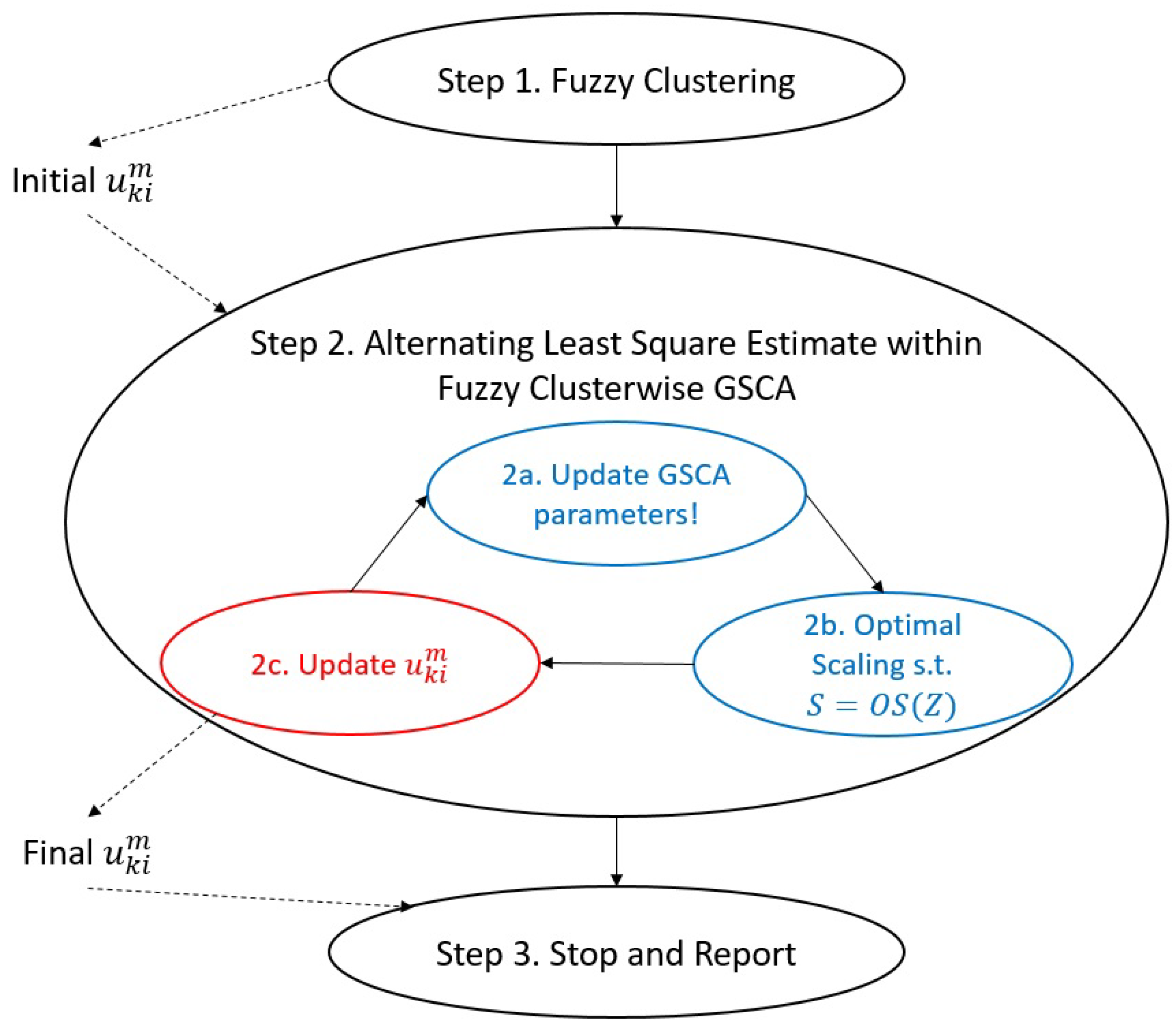
Ryoo, Park, and Kim [4] applied fuzzy clusterwise GSCA to binary or ordinal observed data by combining optimal scaling with the fuzzy clustering algorithm to identify heterogeneous subgroups. The model provided is similar as latent class analysis (LCA), a factor-based model identifying heterogeneous subgroups under binary or ordinal observed data. The algorithm depicted in Figure 1 starts with fuzzy clustering in Step 1, which gives initial membership probability, $u_{ki}^m$. In step 2, after estimating the parameters of GSCA and applying the optimal scaling, $s_j=\omega \left(z_j\right)$, we also update the $u_{ki}^m$. This alternating process will be repeated until the parameters converge. When all parameters were estimated in Step 3, we utilize the parameters to define the characteristics of clusters and assign the membership based on posterior probabilities, $u_{ki}^m$.

It should be noted that, due to the nature of the difference between component-based LCA, i.e., fuzzy clusterwise GSCA for discrete data, and factor-based LCA, there is no one-to-one correspondence between the membership assignments in component-based LCA and factor-based LCA. One of the reasons causing the discrepancy would be estimation methods. That is, the fuzzy clustering GSCA identifies the distances from the centroids, whereas factor-based LCA relies on the likelihood function. Thus, instead of competing with each other, it is reasonable to suggest that researchers select one of the approaches, either fuzzy clustering GSCA for discrete data or factor based LCA, following Hwang, Takane, and Jung [14], who discussed the conceptual difference between two approaches, namely the component-based SEM and the factor-based SEM, respectively, for such cases.

2.6. Model Evaluation

For the overall model evaluation in fuzzy clusterwise GSCA, FIT and AFIT indices were used to evaluate fitted GSCA models (see [2] for more details). FIT and AFIT are interpreted as the variance explained by the fitted model, like R squared and adjusted R squared, in regression analysis. Thus, for the larger FIT and AFIT, the more of the variance is explained. In this study, we mainly focus on model evaluation to enumerate the optimal number of clusters (or latent classes) indicating the heterogeneity of the population given. Accordingly, two additional model evaluation tools used in fuzzy clusterwise GSCA, modified partition coefficient (MPC), and normalized classification entropy (NCE), are our interest as well. For MPC and NCE, the smaller the better. These indexes are somewhat limited to be used in the fuzzy clustering context. Therefore, we will extend model evaluation tools for fuzzy clusterwise GSCA by employing cluster validity indexes known in fuzzy clustering ([6,15]).

3. Method

To enumerate the clusters in fuzzy clustering, many indexes have been used but can be classified based on two criteria: compactness (intra-cluster consistency) and separation (inter-cluster consistency) [6]. However, not all of the indexes can also be used in fuzzy clusterwise GSCA because fuzzy clusterwise GSCA accounts for not only distance from the centroids but also characteristics of each cluster identified by observed indicators via the probabilities of occurring the event associated with the indicator. In addition, fuzzy clusterwise GSCA accounts for the effects of covariates and/or grouping variables as statistical modeling, which is called latent class regression ([16,17,18]). Thus, cluster validation indexes dealing with various structures in fuzzy clusterwise GSCA should be considered. In the section, we review cluster validity indexes that have been used within fuzzy clustering with two validity index categories: using the membership values only and using both the membership values and the dataset ([6,15]). Moreover, we also review two indexes, MPC and NCE, that have been used in fuzzy clusterwise GSCA. Overall, we selected eight index candidates, two model fit indexes, and six cluster validity indexes that can be used for enumerating the optimal number of clusters within fuzzy clusterwise GSCA.

3.1. Cluster Validity Indexes

To find the optimal number of clusters using the membership probability and the data given, we consider the following six indexes. Although Wang and Zhang [6] listed more than 20 indexes, we did not list all of them (1) because they said there is no dominating index in the study using both empirical and simulated datasets and (2) because not all the indexes work in fuzzy clusterwise GSCA. Let N and C be sample size and number of clusters in the formulae below:

(a)

Dave’s modified partition coefficient (MPC; [15]): Using partition coefficient defined by $PC=\frac{1}{N}{\sum }_{k=1}^C{\sum }_{i=1}^N{u}_{ki}^{2}andPC\in \left[\frac{1}{C},1\right]$, Dave defined the MPC, also known as fuzzy performance index (FPI), as

$$MPC=1-\frac{C·(1-PC)}{C-1},$$

(4)

where C is the number of clusters. As a modification of the bias of PC such that there is a monotonic tendency [15], MPC performs well with a criterion—the larger the better.

(b)

Bezdek’s normalized classification entropy (NCE; [19]): Using partition entropy $\left(PE=-\frac{1}{N}{\sum }_{k=1}^C{\sum }_{i=1}^N{u}_{ki}log{u}_{ki}\right)$, Bezdek defined the NCE as

$$NCE=\frac{PE}{logC},$$

(5)

which is also recommended by Roubens [5]. The criterion that smaller is better is applied in the NCE. Based on the partition entropy, Bezdek [13] also defined the normalized partition entropy (NPE) as

$$NPE=\frac{N·PE}{N-C}.$$

(6)

The same criterion as in the NCE is applied to NPE.

(c)

Chen and Linkens’ validity index (CLVI; [20]): They defined the CLVI as

$$CLVI=\frac{1}{N}\sum _{i=1}^N\underset{k}{max}\left(u_{ki}\right)-\frac{1}{C^{*}}\sum _{k=1}^{C-1}\sum _{l=k+1}^C\left[\frac{1}{N}\sum _{i=1}^{N}min(u_{ki},u_{li})\right]$$

(7)

where $C^{*}={\sum }_{i=1}^{C-1}k$. An optimal cluster number C is obtained at the max of CLVI. The first term indicates the compactness within a cluster while the second term indicates the separation between clusters. When the first term is larger and the second term is lower, the clusters are compact as well as clearly separable from the other clusters. Thus, the larger the CLVI is, the better.

(d)

Fukuyama and Sugeno proposed an index (FS; [21]):

$$\begin{array}{cc}\hfill FS& =J_m(u,v)-K_m(u,v)\hfill \\ \hfill & =\sum _{k=1}^C\sum _{i=1}^N{u}_{ki}^m\left|\right|x_i-v_k{\left|\right|}^2-\sum _{k=1}^C\sum _{i=1}^N{u}_{ki}^m\left|\right|v_k-\overline{v}{\left|\right|}^2,\hfill \end{array}$$

(8)

where $\overline{v}={\sum }_{k=1}^C\frac{v_k}{C}$. The first term describes both the fuzziness in each cluster and the compactness of data, and the second term describes the fuzziness of the clusters with the distance of centroids from the grand mean of the data. We can find an optimal C at $\underset{2\le C\le N-1}{min}FS$.

(e)

Gath and Geva’s fuzzy hypervolume validity index (FHV; [22]): They defined the FHV as

$$FHV=\sum _{k=1}^C{\left[det\left(F_k\right)\right]}^2,$$

(9)

where $F_k=\frac{{\sum }_{i=1}^N{u}_{ki}^m(x_i-v_k){(x_i-v_k)}^T}{{\sum }_{i=1}^N{u}_{ki}^m}$. The matrix $F_k$ denotes the fuzzy covariance matrix of cluster k, and $det\left(F_k\right)$ is the determinant of the matrix $F_k$. The smaller the FHV value is the better and, thus, we find an optimal C at $\underset{2\le C\le N-1}{min}FHV$.

3.2. Holistic Approach to Enumerate the Number of Clusters

In fuzzy clustering, the literature on finding the optimal number of clusters indicated that there is no dominant index outperforming [6]. Rather, the efficiency of indexes would be dependent on data distribution [15]. Although fuzzy clustering GSCA does include more model specification than fuzzy clustering, it is likely to hold similar property in model evaluation. In this study, we are not only examining the efficiency of indexes but also investigating a holistic criterion that performs well and in a stable manner.

3.3. Simulation Design

To examine the efficiency of cluster validation indexes: FIT, AFIT, FPI, NCE, NPE, CLVI, FS, and FHV, five variables were considered in this simulation:

• three levels of sample size (N),
• three levels of the number of latent classes/clusters (K),
• two levels of the number of indicators (V),
• three levels of prevalence of the cluster membership (T), and
• three levels of error rate in the cluster structure (ER).

In total, 162 $(=3\times 3\times 2\times 3\times 3)$ simulation conditions were employed, and they are summarized in

Table 1. Study conditions for the simulation.

Variable	Number of Conditions	Condition
Sample size (N)	3	200, 500, and 1000
Number of cluster (K)	3	2, 4, and 6
Number of indicators (V)	2	6 and 9
Prevalence of	3	(T1) Equally clustered:
cluster membership (T)		${\lambda }_k=\frac{1}{K}$ where $1\le k\le K$
		(T2) One cluster has large proportion:
		${\lambda }_1=0.6$ and ${\lambda }_k=\frac{0.4}{K-1}$ where $1\le k\le K$
		(T3) One cluster has small proportion:
		${\lambda }_1=0.1$ and ${\lambda }_k=\frac{0.9}{K-1}$ where $1\le k\le K$
Error rates (ER)	3	5%, 10%, and 15%

. Based on the simulation conditions, 100 responses were generated and, then, we fitted fuzzy clusterwise GSCA into the response data. The current study designed the simulation conditions based on the previously conducted simulation studies in component-based latent class analysis including [23,24].

3.3.1. Sample Size

Three levels of sample size were used in the simulation study: 200, 500, and 1000, representing small, medium, and large samples. Brusco et al. [23] investigated the cases with relatively small sample sizes (100, 200, and 400); however, the fit indices of their study were not distinguishable depending on the sample sizes. Thus, the current study explored the broader range of sample sizes.

3.3.2. The Number of Classes/Clusters

Two, four, and six classes were investigated to examine the efficiency of cluster validation indexes, which covers most of results from latent class analysis. Previous studies ([23,24]) considered two additional numbers of classes, 3 and 5, so that it covers all the cases from 2 to 6. However, the cases of 3 and 5 did not give any additional trend in the examination of the efficiency. Thus, we exclude the cases in this study.

3.3.3. The Number of Indicators

The number of indicators and response patterns adapted from the previous studies ([23,24]) was applied in this study. The response patterns in

Table 2. Response patterns for combinations of the number of classes (K) and the number of item indicators (V).

Number of Cluster	Number of Indicators (V = 6)	Number of Indicators (V = 9)
K = 2	(1, 1, 1, 1, 0, 0)	(1, 1, 1, 1, 1, 1, 0, 0, 0)
	(0, 0, 1, 1, 1, 1)	(0, 0, 0, 1, 1, 1, 1, 1, 1)
K = 4	(1, 1, 1, 1, 0, 0)	(1, 1, 1, 1, 1, 1, 0, 0, 0)
	(0, 0, 1, 1, 1, 1)	(0, 0, 0, 1, 1, 1, 1, 1, 1)
	(0, 0, 0, 0, 1, 1)	(0, 0, 0, 0, 0, 0, 1, 1, 1)
	(1, 1, 0, 0, 0, 0)	(1, 1, 1, 0, 0, 0, 0, 0, 0)
K = 6	(1, 1, 1, 1, 0, 0)	(1, 1, 1, 1, 1, 1, 0, 0, 0)
	(0, 0, 1, 1, 1, 1)	(0, 0, 0, 1, 1, 1, 1, 1, 1)
	(0, 0, 0, 0, 1, 1)	(0, 0, 0, 0, 0, 0, 1, 1, 1)
	(1, 1, 0, 0, 0, 0)	(1, 1, 1, 0, 0, 0, 0, 0, 0)
	(0, 0, 1, 1, 0, 0)	(0, 0, 0, 1, 1, 1, 0, 0, 0)
	(1, 1, 0, 0, 1, 1)	(1, 1, 1, 0, 0, 0, 1, 1, 1)

were directly used to generate data under the aforementioned conditions of sample sizes and the number of classes. For example, when sample size is 200 and samples are equally clustered in two classes, the response of the first 100 samples with six indicators is $(1,1,1,1,0,0)$, and the next response of 100 samples is $\left(0,0,1,1,1,1\right)$, assuming there is no error rate.

3.3.4. Prevalence of Class Membership

There are three different types of prevalence, T1, T2, and T3 in Table 1. The first one (T1) is equally clustered, given the number of classes. The second possible prevalence (T2) is that one class has a dominant number of examinees (60%) and the other classes have equally clustered within the leftover (40%). For example, for $K=4$, the first cluster (C1), the second cluster (C2), the third cluster (C3), and the fourth cluster (C4) consist of 60%, 13.3%, 13.3%, and 13.3%, respectively. Lastly, we considered the case where one group has a small proportion. For example, for $K=6$, C1, C2, C3, C4, C5, and C6 consist of 18%, 18%, 18%, 18%, 18%, and 10%. The details of formulas are presented in Table 1. These study conditions follow Brusco et al. [23].

3.3.5. Error Rates

All samples within a class would not have the exact same response patterns but, instead, the variations of the responses generated were determined by three levels of error rates: 5%, 10%, and 15%. As the higher error rates, such as 20% or 30%, caused poor cluster recovery in a previous study [24], the current study used relatively low error rates, following Brusco et al. [23]. Once an error rate is determined, the samples with the error rate were randomly selected and one of the indicator responses was manipulated as follows: If the original response was 0, it was changed to 1 and vice versa. Selection of indicators manipulated was also random.

Once the data were generated, we estimated the generated responses with different assigned cluster numbers in order to evaluate how many clusters would be best given each study condition. When the true number of clusters was 2 and 4, we fitted fuzzy clusterwise GSCA using a R package, gscaLCA [25], with 2-solution to 4-solution and 2-solution to 6-solution, respectively. When a true number of clusters was 6, we fitted fuzzy clusterwise GSCA with 4-solution to 8-solution.

4. Results

After fitting a fuzzy clusterwise GSCA into 100 replications for each condition (total of 162 conditions), we examined the efficiency of 8 cluster validity indexes, FIT, AFIT, MPC, NCE, NPE, CLVI, FS, and FHV. In this section, we summarized the results of (1) $K=4$ and $N=500$ and (2) $K=6$ and $N=200$ representing the medium number of clusters and the medium number of sample size and the large number of clusters and a small number of sample size. The first case informs the trend of our findings from the 162 conditions, which allows us to formulate our findings as well as propose a holistic criterion. The latter case informs the stability of our findings because the case is most vulnerable due to the complexity in the clusters and the sample variation from the small sample.

4.1. FIT-FHV Method

As Wang W. et al. [6,15] pointed out, any single index was not sufficient enough to identify the true number of clusters due to the dependency of data distribution in the efficiency. However, when the model evaluation tools in GSCA were controlled, it was clear that a holistic search performs well in identifying the true number of clusters.

Table 3. Simulation results of $K=4$, $N=500$, $V=6$ items, and $ER=15\%$.

T	# of Clusters	FIT	AFIT	MPC	NCE	NPE	CLVI	FS	FHV
	C = 2	0.999	0.999	0.478	0.579	0.403	0.616	14,398.987	40.668
	C = 3	0.996	0.996	0.847	0.159	0.176	0.884	16,516.787	71.985
T1	C = 4	0.997	0.997	0.568	0.395	0.552	0.697	−744.482	22.694
	C = 5	0.783	0.766	0.682	0.282	0.458	0.780	−5009.347	18.840
	C = 6	0.820	0.803	0.751	0.212	0.384	0.831	−6074.661	41.356
	C = 2	0.996	0.996	0.838	0.210	0.146	0.901	27,725.400	36.559
	C = 3	0.996	0.995	0.656	0.343	0.379	0.773	20,992.742	43.942
T2	C = 4	0.995	0.995	0.706	0.273	0.382	0.802	11,024.970	28.450
	C = 5	0.883	0.874	0.648	0.287	0.466	0.762	−1184.398	22.112
	C = 6	0.920	0.912	0.733	0.211	0.383	0.825	−7349.990	15.296
	C = 2	0.999	0.999	0.520	0.541	0.377	0.657	15,769.265	42.760
	C = 3	0.998	0.998	0.817	0.201	0.222	0.861	5193.876	27.043
T3	C = 4	0.995	0.994	0.792	0.203	0.284	0.852	363.110	13.909
	C = 5	0.791	0.776	0.833	0.156	0.254	0.881	−3904.634	10.771
	C = 6	0.856	0.843	0.863	0.126	0.228	0.904	−7034.518	18.275

summarized the result of $K=4$, $N=500$, $V=6$ items, and $ER=15\%$ over all three types of distributions, $T=1,2,$ and 3. Note that the symbol, C, in Table 3 is the number of clusters used for the estimation.

FIT and AFIT performed similarly and indicated a big drop after C reaches the true number of cluster K. More than 0.2 were dropped at $C=5$ in T1 and T3 while more than 0.1 was dropped at $C=5$ in T2. However, both FIT and AFIT did not show any discrepancy for $C=2$, $C=3$, and $C=4$ (true number of clusters). Although FHV showed small values when $C=4$, there were several cases indicating lower values ($C\ge 4$). Interestingly, none of the FHV values for $C\le 3$ were lower than the FHV of $C=4$. Thus, we found that the smallest FHV indicates the true number of clusters if we consider the index FHV within the range of C whose FIT and AFIT’s values are stable and high. Let us call this holistic criterion as a FIT-FHV method. Only 11 conditions out of 162 simulation conditions did not follow the FIT-FHV criterion. However, those 11 conditions were associated with a small sample size of $N=200$ where we rarely fit the fuzzy clusterwise GSCA into such relatively small data.

FS would be an index to be considered similar in the FIT-FHV method, but FS indicated a monotonicity, which was a drawback in the traditional measures of partition coefficient (PC) and partition entropy (PE) shown in [15]. Thus, it requires further investigation regarding the index FS. MPC, NCE, NPE, and CLVI indicated neither the true number of clusters nor any consistency in the selection.

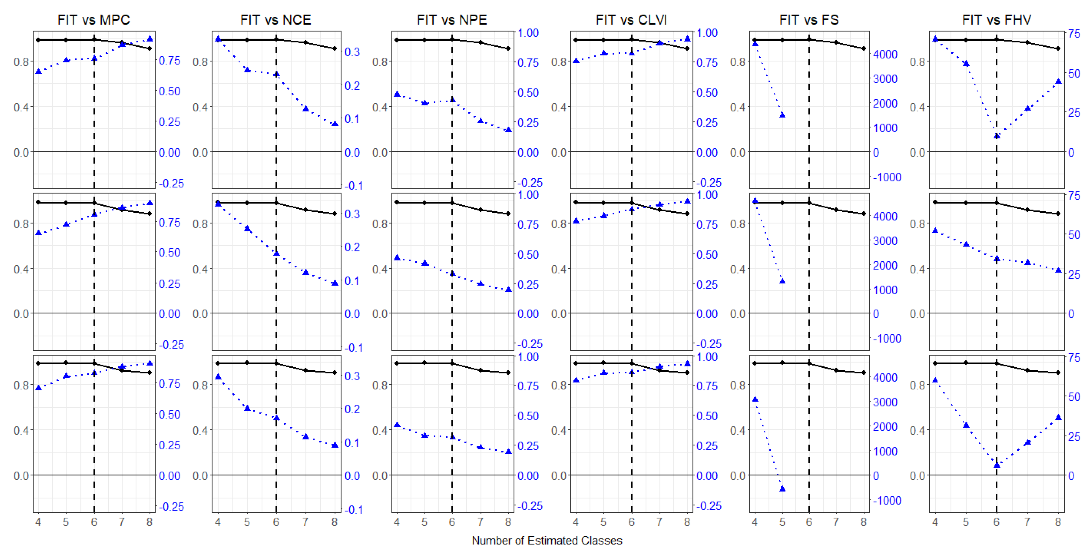
The property of the FIT-FHV criterion was also observed in Figure 2. Six indexes (blue) were plotted with the profile of FIT (black), where the first row indicates the equally clustered (T1), the second and third row describe the one cluster that has a large proportion (T2), and one cluster has a small proportion (T3) condition, respectively. The profile of FIT clearly showed the big drop when $C>K$. If we considered $C\le K$, FHV was the smallest number when $C=K$. Again, FS could also be considered, but the range of values were relatively large from negative to positive. The FIT-FHV method worked well for larger samples, $N=1000$, larger indicators, $V=9$, and smaller ER such as 5% and 10%.

4.2. Stability of the FIT-FHV Method

Furthermore, we examined the stability of the FIT-FHV method by exploring the most vulnerable condition such that $K=6$ and $N=200$ (

Table 4. Simulation results of $K=6$, $N=200$, $V=6$ items, and $ER=15\%$.

T	# of Clusters	FIT	AFIT	MPC	NCE	NPE	CLVI	FS	FHV
	C = 4	0.980	0.977	0.648	0.335	0.474	0.757	4360.678	70.794
	C = 5	0.981	0.977	0.741	0.243	0.401	0.818	1459.266	55.370
T1	C = 6	0.988	0.985	0.758	0.231	0.426	0.820	−2711.276	9.458
	C = 7	0.962	0.950	0.867	0.127	0.255	0.904	−3627.897	26.785
	C = 8	0.911	0.877	0.913	0.081	0.175	0.937	−4281.379	43.793
	C = 4	0.982	0.979	0.651	0.326	0.461	0.769	4563.684	51.954
	C = 5	0.971	0.965	0.720	0.252	0.416	0.813	1278.064	43.150
T2	C = 6	0.971	0.963	0.804	0.177	0.327	0.869	−2523.121	34.236
	C = 7	0.912	0.884	0.859	0.121	0.243	0.907	−4044.144	31.770
	C = 8	0.882	0.836	0.897	0.089	0.192	0.932	−4714.370	26.868
	C = 4	0.988	0.986	0.704	0.293	0.414	0.791	3051.090	59.722
	C = 5	0.990	0.988	0.804	0.198	0.327	0.851	−591.218	31.221
T3	C = 6	0.989	0.986	0.829	0.170	0.314	0.859	−3049.061	5.911
	C = 7	0.927	0.903	0.883	0.113	0.229	0.905	−3481.078	20.337
	C = 8	0.906	0.869	0.908	0.088	0.190	0.927	−3957.682	35.981

). Compared with the previous condition, the case of $K=6$ and $N=200$ has two additional clusters but only 200 samples. Although the drops in FIT and AFIT were not bigger than the previous case, we observed the drops in each T. Based on the C selected from the FIT criterion, we easily identified the true number of clusters by examining the FHV values. The FIT-FHV method worked well even in the most vulnerable condition in the simulation study.

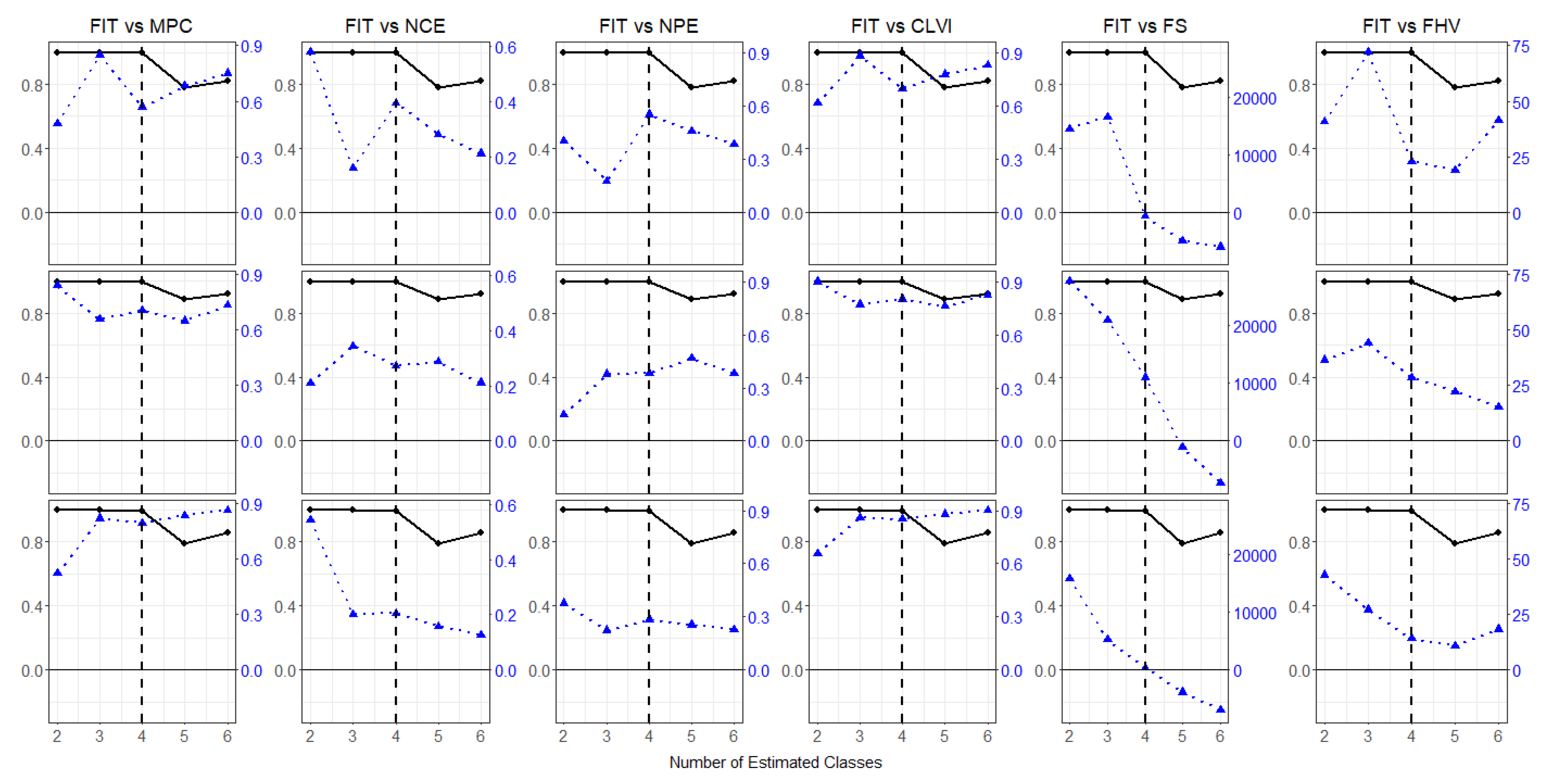
Figure 3 indicated that MPC, NCE, NPE, CLVI, and FS may work for a criterion, similar to the FIT-FHV method. However, all of the five fit indexes showed monotonicity. Again, FS indicated more severe negative values as C increased. Thus, we would conclude that the FIT-FHV method outperforms in identifying the true number of clusters in this simulation.

4.3. Prevalence of Clusters When C Is Assumed to be the Optimal Number of Clusters

In fuzzy clusterwise GSCA, it is also of importance that the selected number of clusters, by the FIT-FHV method, consists of similar proportions as in the true population.

Table 5. Prevalence of $K=4$, $N=500$, $V=6$ items, and $ER=15\%$.

T	# of Clusters	C = 1	C = 2	C = 3	C = 4	C = 5	C = 6
	C = 2	96.28	3.72
	C = 3	53.39	46.60	0.01
T1	C = 4	38.73	29.21	18.78	13.28
	C = 5	31.48	25.67	22.36	19.36	1.13
	C = 6	29.38	25.22	22.04	19.08	3.21	1.07
	C = 2	99.71	0.29
	C = 3	71.94	20.78	7.28
T2	C = 4	64.86	16.95	13.86	4.33
	C = 5	55.93	18.16	14.80	9.69	1.42
	C = 6	53.03	16.88	14.48	11.34	2.64	1.62
	C = 2	91.52	8.48
	C = 3	37.72	33.55	28.74
T3	C = 4	35.34	32.15	28.27	4.24
	C = 5	34.71	30.80	26.74	6.69	1.07
	C = 6	33.50	29.02	26.08	8.00	2.40	1.00

and

Table 6. Prevalence of $K=6$, $N=200$, $V=6$ items, and $ER=15\%$.

T	# of Clusters	C = 1	C = 2	C = 3	C = 4	C = 5	C = 6	C = 7	C = 8
	C = 4	50.98	29.86	15.56	3.61
	C = 5	37.09	24.22	17.86	13.53	7.31
T1	C = 6	23.31	19.28	17.15	15.12	13.62	11.54
	C = 7	19.32	17.28	15.93	14.99	13.77	12.98	5.75
	C = 8	17.62	16.20	15.31	14.68	13.84	12.94	6.34	3.08
	C = 4	63.70	21.00	10.47	4.85
	C = 5	57.73	17.92	11.46	7.93	4.97
T2	C = 6	53.02	13.29	10.73	9.23	7.86	5.88
	C = 7	52.21	11.55	9.65	8.53	7.47	6.65	3.95
	C = 8	51.93	10.43	8.94	8.13	7.41	6.59	4.07	2.53
	C = 4	44.52	26.87	17.92	10.70
	C = 5	31.09	20.82	18.28	16.19	13.63
T3	C = 6	23.05	19.88	17.91	16.22	14.80	8.16
	C = 7	20.59	18.64	17.37	16.08	14.70	8.96	3.67
	C = 8	19.65	17.66	16.74	15.82	14.57	9.09	4.22	2.27

summarized the proportions for the two conditions aforementioned. For the case of $K=4$ and $N=500$, T1, T2, and T3 should consist of $(25\%,25\%,25\%,25\%)$, $(60\%,13.3\%,13.3\%,13.3\%)$, and $(30\%,30\%,30\%,10\%)$. In T1, all of the Cs except $C=4$ included a very small proportion at the last cluster. In practice, it is hard to characterize a group with such a small proportion. On the other hand, the case of $C=4$ included 13.38% that was much smaller than 25% but was not comparable with the others. In T2, the true dominant group consists of 60% and we found that the cases of $C\ge 4$ held a close proportion. However, the last two groups of $C=5$ and $C=6$ were 1.42% and 1.62%, respectively. Such lower prevalence rates would not be meaningful. These results indicate that the FIT-FHV method works well. In T3, the true last cluster should consist of 10%, which may indicate that $C=2$ is a good proxy. However, its FHV was always higher than $C=4$, which means that the classification would hold weak compactness (intra-cluster consistency). It is clear that $C=4$ in T3 was closer to the true prevalence than $C=3$ (not identifying the fourth cluster), $C=5$ (too low prevalence in the last cluster), and $C=6$ (too low prevalence in the last two clusters).

Even though we consider the most vulnerable case of $K=6$ and $N=200$, the same trend as in the case of $K=4$ and $K=500$ was observed. For the case of $K=6$ and $N=200$, T1, T2, and T3 should consist of $(16.7\%,16.7\%,16.7\%,16.7\%,16.7\%,16.7\%)$, $(60\%,8\%,8\%,8\%,8\%,8\%)$, and $(18\%,18\%,18\%,18\%,18\%,10\%)$. In T1, all of the Cs except $C=6$ included a very small proportion at the last cluster. On the other hand, the case of $C=6$ included 11.54% that was much smaller than 16.7% but was not comparable with the others. In T2, where the true dominant cluster consists of 60%, we found that the cases of $C\le 6$ held close proportions to the true ones. However, the second groups of $C=4$ and $C=5$ were relatively higher than 8% as 21.00% and 17.39%, respectively. Thus, it would not be meaningful. In T3, where the true last group consists of 10%, the results may indicate that $C=4$ is good proxy. However, its FHV was always higher than $C=6$, which means that the classification would hold weak compactness (intra-cluster consistency). Overall, $C=K$ approximates the true prevalences.

4.4. Real World Application in the Field of Public Health

To investigate the applicability of the proposed FIT-FHV method in a real world data, we fitted fuzzy clusterwise GSCA into Add Health data [26]. The Add Health data used in this study consists of five indicators which are dichotomous responses. For the detailed explanations of Add Health data, please refer to the package gscaLCA [4]. The sample size of the data are 5114, but we explored the smaller sample sizes cases corresponding to the sample sizes used in the simulation study. For the smaller sample sizes (250, 500, and 1000), we randomly selected observations out of the entire samples. For each sample size data, we fitted fuzzy clusterwise GSCA over the number of clusters from 2 to 8.

The fit indexes to determine the optimal number of clusters were summarized in

Table 7. FIT Indexes of empirical data analysis results.

Sample Sizes	# of Clusters	FIT	AFIT	MPC	NCE	NPE	CLVI	FS	FHV
N = 250	C = 2	0.9924	0.9920	0.226	0.824	0.576	0.421	3843.301	40.657
	C = 3	0.9811	0.9797	0.522	0.506	0.562	0.669	2533.668	28.853
	C = 4	0.9771	0.9747	0.559	0.458	0.646	0.665	1013.757	25.313
	C = 5	0.9606	0.9551	0.792	0.209	0.343	0.868	1364.492	33.586
	C = 6	0.9361	0.9252	0.730	0.261	0.478	0.787	−427.198	15.310
	C = 7	0.9364	0.9234	0.817	0.172	0.345	0.865	−584.003	21.159
	C = 8	0.9474	0.9348	0.941	0.054	0.117	0.960	−2022.800	19.674
N = 500	C = 2	0.9973	0.9973	0.338	0.728	0.507	0.532	4369.003	22.563
	C = 3	0.9937	0.9935	0.574	0.464	0.513	0.720	4115.353	31.469
	C = 4	0.9887	0.9881	0.597	0.424	0.593	0.678	−884.863	18.487
	C = 5	0.9791	0.9778	0.736	0.264	0.430	0.802	−3310.829	11.697
	C = 6	0.9721	0.9699	0.783	0.213	0.386	0.833	−3623.326	10.524
	C = 7	0.9699	0.9671	0.922	0.076	0.150	0.947	−4895.632	22.753
	C = 8	0.9727	0.9698	0.898	0.097	0.205	0.918	−8078.892	2.895
N = 1000	C = 2	0.9987	0.9986	0.306	0.761	0.529	0.529	9036.031	22.017
	C = 3	0.9961	0.9960	0.577	0.463	0.510	0.709	6404.905	27.542
	C = 4	0.9949	0.9948	0.617	0.404	0.562	0.700	−6839.396	9.283
	C = 5	0.9870	0.9865	0.746	0.251	0.407	0.803	−7828.256	9.667
	C = 6	0.9859	0.9854	0.801	0.195	0.352	0.851	−4721.540	15.512
	C = 7	0.9854	0.9847	0.856	0.136	0.266	0.892	−12,560.950	9.850
	C = 8	0.9850	0.9842	0.899	0.095	0.198	0.917	−15,097.641	2.638
N = 5114	C = 2	0.9997	0.9997	0.318	0.750	0.520	0.533	50,391.382	22.212
	C = 3	0.9993	0.9993	0.540	0.500	0.550	0.669	28,373.742	21.772
	C = 4	0.9983	0.9983	0.668	0.342	0.475	0.760	−3925.974	17.109
	C = 5	0.9976	0.9975	0.747	0.251	0.405	0.808	−39,992.537	9.340
	C = 6	0.9974	0.9974	0.805	0.191	0.343	0.848	−42,944.767	10.994
	C = 7	0.9974	0.9974	0.993	0.009	0.018	0.995	−37,415.660	20.548
	C = 8	0.9966	0.9966	0.905	0.088	0.183	0.930	−76,661.158	5.493

. The results showed that there were drops regarding FIT and AFIT at $C=5$ regardless of the sample sizes. Although the drops of FIT and AFIT were not very distinguishable in the large sample size 5114, compared to the small sample size cases, they were still noticeable within the result of sample size 5114. In addition, the results showed that the FHV values were smallest at $C=4$ for four different sample size data sets when considering only $C\le 4$ based on the drops. While applying the FIT-FHV method into the results, we would conclude that $C=4$ is the optimal clusters in fitting fuzzy clusterwise GSCA in this dataset regardless of sample sizes. In addition, the empirical analysis results demonstrated that MPC, NCE, NPE, CLVI, and FS showed the monotonic tendency like the simulation results. That is, the results of empirical data analysis confirmed that the proposed FIT-FHV method performed well.

In

Table 8. Prevalence of empirical data analysis results.

Sample Sizes	# of Clusters	C = 1	C = 2	C = 3	C = 4	C = 5	C = 6	C = 7	C = 8
N = 250	C = 2	56.68	43.32
	C = 3	55.47	29.55	14.98
	C = 4	37.65	23.08	21.46	17.81
	C = 5	33.20	24.29	18.62	14.17	9.72
	C = 6	24.70	19.84	19.03	16.60	14.17	5.67
	C = 7	27.13	16.60	15.38	14.98	14.57	7.29	4.05
	C = 8	20.24	17.81	15.38	14.57	14.17	8.91	5.67	3.24
N = 500	C = 2	56.57	43.43
	C = 3	46.67	34.75	18.59
	C = 4	32.93	28.48	20.00	18.59
	C = 5	31.11	23.03	18.59	15.96	11.31
	C = 6	22.22	20.81	18.99	16.36	13.94	7.68
	C = 7	27.27	19.39	13.74	13.33	10.71	9.49	6.06
	C = 8	20.81	18.59	16.97	13.94	10.71	7.68	6.06	5.25
N = 1000	C = 2	55.16	44.84
	C = 3	47.47	33.70	18.83
	C = 4	34.82	27.23	19.13	18.83
	C = 5	29.45	25.10	18.83	14.88	11.74
	C = 6	26.01	21.96	19.03	15.38	11.74	5.87
	C = 7	24.39	18.93	14.88	14.57	14.37	6.98	5.87
	C = 8	21.05	18.42	17.71	14.07	10.93	7.09	5.87	4.86
N = 5114	C = 2	55.09	44.91
	C = 3	47.73	32.02	20.25
	C = 4	29.59	26.69	24.14	19.58
	C = 5	29.45	25.05	19.52	15.42	10.56
	C = 6	23.02	22.38	19.64	18.38	10.56	6.02
	C = 7	28.54	19.58	15.77	13.98	9.91	6.85	5.37
	C = 8	21.08	20.23	15.79	14.11	10.56	6.89	6.61	4.72

, the results of prevalence in the empirical data analysis are presented. Table 8 showed that the proportions of each cluster were similar overall for different sample sizes, given each number of clusters, although there is some variability. The distinguishable variabilities were usually observed with the sample size 250. When $C=4$, the selected number of clusters based on the FIT-FHV method, the ranges of prevalence except for the sample size 250 were 29.59 to 32.93%, 26.69 to 28.48%, 19.13 to 20.00%, and 18.83 to 19.58% for each cluster, respectively. With the sample size 250, the prevalence is 37.65%, 23.08%, 21.24%, and 17.81%. These differences among the results of the sample sizes would be because of either randomness or the instability of small sample size like the results of the simulation study.

5. Discussion and Conclusions

In this simulation study, we found that each cluster validation index with its criterion given did not perform well. Some indexes including FS still showed monotonicity. These results are consistent with [6,15] studies. Among the eight indexes compared, FHV performs better although some of high-solutions (meaning that its number of clusters is higher than the true number of clusters) hold lower FHV. As fuzzy clusterwise GSCA is a complex model including both fuzzy clustering and GSCA, it would not be optimistic to get a single index that outperforms over the other indexes. Accordingly, we focused on finding a holistic criterion to identify the true number of clusters with a combination of a couple of indexes. This strategy allows us to find the FIT-FHV method that identifies the true number of clusters for most of the 162 simulation conditions. Here is the FIT-FHV method:

• (Step 1:) Find a drop point on FIT and AFIT. The last point of the higher levels indicate the max of the range where the true number of clusters is located.
• (Step 2:) Find the smallest FHV within the range found in Step 1, which gives the optimal number of clusters.
• (Step 3:) Explore the prevalence distribution of clusters and confirm that none of the prevalence rates are too low.

5.1. Limitation

This study finding of the FIT-FHV method would not be generalizable to both fuzzy clustering and GSCA. Even if we consider fuzzy clusterwise GSCA, it should be noted that this simulation study assumed $m=2$. Another limitation is that data distribution generated in this simulation study only accounts for the variations with error rates, 5%, 10%, and 15%. As [15] pointed out, the specific data distribution would affect the performance of the FIT-FHV method. Lastly, the type of observed indicators was binary although fuzzy clusterwise GSCA covers ordinary and continuous indicators. All of these limitations are our future research topics so that the FIT-FHV method works for all of fuzzy clusterwise GSCA.

The cluster validation problem is a common issue in fuzzy clustering in general. To resolve this issue, researchers have recently developed a variety of tools in clustering; for example, Bayesian neuro-fuzzy modeling for estimating gas turbine compressor discharge temperature [27]. At the same time, researchers also focused on utilizing the classical cluster quality indexes, for example, in selecting optimal features for cross-fleet analysis and fault diagnosis of industrial gas turbines [28]. This study mainly focused on utilizing the classical cluster quality indexes in structural equation modeling dealing with many social/behavioral sciences and medical fields. Due to the combination of fuzzy clustering and generalized structured component analysis, it should be noted that the proposed method, FIT-FHV, may not outperform the other cluster indexes. In the same fashion, it is out of our scope to compare the efficiency between the FIT-FHV and the other indexes used in fuzzy clustering.

5.2. Concluding Remarks

Although fuzzy clustering and generalized structured component analysis have been widely used as a statistical model in the inferential statistics, the fuzzy clusterwise GSCA has suffered from identifying the optimal number of clusters. The new method, called the FIT-FHV method, proposed in this study should help researchers identify the optimal number of clusters in fuzzy clusterwise GSCA. Furthermore, the FIT-FHV method could be beneficial to mixture models in general.

References

1. Muthén, B. Latent variable mixture modeling. In New Developments and Techniques in Structural Equation Modeling; Marcoulides, G.A., Schumaker, R.E., Eds.; Erlbaum: Mahwah, NY, USA, 2001; pp. 1–33. [Google Scholar]
2. Hwang, H.; Takane, Y. Generalized Structured Component Analysis: A Component-Based Approach to Structural Equation Modeling; CRC Press: Boca Raton, FL, USA, 2014. [Google Scholar]
3. Hwang, H.; DeSarbo, S.W.; Takane, Y. Fuzzy clusterwise generalized structured component analysis. Psychometrika 2007, 72, 181–198. [Google Scholar] [CrossRef] [Green Version]
4. Ryoo, J.H.; Park, S.; Kim, S. Categorical latent variable modeling utilizing fuzzy clustering generalized structured component analysis as an alternative to latent class analysis. Behaviormetrika 2020, 47, 291–306. [Google Scholar] [CrossRef]
5. Roubens, M. Fuzzy clustering algorithms and their cluster validity. Eur. J. Oper. Res. 1982, 10, 294–301. [Google Scholar] [CrossRef]
6. Wang, W.; Zhang, Y. On fuzzy cluster validity indices. Fuzzy Sets Syst. 2007, 158, 2095–2117. [Google Scholar] [CrossRef]
7. Bezdek, J.C. Numerical taxonomy with fuzzy sets. J. Math. Biol. 1974, 1, 57–71. [Google Scholar] [CrossRef]
8. Jöreskog, K.G. A general method for estimating a linear structural equation system. In Structural Equation Models in the Social Sciences; Goldberger, A.S., Duncan, O.D., Eds.; Seminar Press: New York, NY, USA, 1973. [Google Scholar]
9. Hwang, H.; Takane, Y. Nonlinear generalized structured component analysis. Psychometrika 2010, 37, 1–14. [Google Scholar] [CrossRef]
10. McDonald, R.P. Test Theory: A Unified Treatment; Lawrence Erlbaum Associates: Mahwah, NY, USA, 1999. [Google Scholar]
11. de Leeuw, J.; Young, F.W.; Takane, Y. Additive structure in qualitative data: An alternating least squares method with optimal scaling features. Psychometrika 1976, 41, 471–503. [Google Scholar] [CrossRef]
12. Young, F.W. Quantitative analysis of qualitative data. Psychometrika 1981, 46, 347–388. [Google Scholar] [CrossRef]
13. Bezdek, J.C. Pattern Recognition with Fuzzy Objective Function Algorithms; Plenum Press: New York, NY, USA, 1981. [Google Scholar]
14. Hwang, H.; Takane, Y.; Jung, K. Generalized structured component analysis with uniqueness terms for accommodating measurement error. Front. Psychol. 2017, 8, 2137. [Google Scholar] [CrossRef] [PubMed] [Green Version]
15. Dave, R.N. Validating fuzzy partitions obtained through c-shells clustering. Pattern Recognit. Lett. 1996, 17, 613–623. [Google Scholar] [CrossRef]
16. Dayton, C.M.; Macready, G.B. Concomitant-variable latent-class models. J. Am. Stat. Assoc. 1988, 83, 173–178. [Google Scholar] [CrossRef]
17. DeSarbo, W.S.; Oliver, R.L.; Rangaswamy, A. A simulated annealing methodology for clusterwise linear regression. Psychometrika 1989, 54, 707–736. [Google Scholar] [CrossRef]
18. Van der Heijden, P.G.M.; Dessens, J.; Bockenholt, U. Estimating the concomitant-variable latent-class model with the EM algorithm. J. Educ. Behav. Stat. 1996, 21, 215–229. [Google Scholar] [CrossRef]
19. Bezdek, J.C. Mathematical models for systematics and taxonomy. In Proceedings of the 8th International Conference on Numerical Taxonomy; Freeman: San Francisco, CA, USA, 1975; pp. 143–166. [Google Scholar]
20. Chen, M.Y.; Linkens, D.A. Rule-base self-generation and simplication for data-driven fuzzy models. Fuzzy Sets Syst. 2004, 142, 243–265. [Google Scholar] [CrossRef] [Green Version]
21. Fukiyama, Y.; Sugeno, M. A new method of choosing the number of clusters for the fuzzy c-means method. In Proceedings of the Fifth Fuzzy Systems Symposium, Kobe, Japan, June 1989; pp. 247–250. Available online: https://jglobal.jst.go.jp/en/detail?JGLOBAL_ID=200902072543924485 (accessed on 14 September 2020).
22. Gath, I.; Geva, A.B. Unsupervised optimal fuzzy clustering. IEEE Trans. Pattern Anal. Mach. Intell. 1989, 11, 773–781. [Google Scholar] [CrossRef]
23. Brusco, M.J.; Shireman, E.; Steinley, D. A comparison of latent class, K-means, and K-median methods for clustering dichotomous data. Psychol. Methods 2017, 22, 563–580. [Google Scholar] [CrossRef] [PubMed]
24. Dimitriadou, E.; Dolničar, S.; Weingessel, A. An examination of indices for determining the number of clusters in binary data sets. Psychometrika 2002, 67, 137–159. [Google Scholar] [CrossRef] [Green Version]
25. Ryoo, J.; Park, S.; Kim, S.; Hwang, H. gscaLCA: Generalized Structure Component Analysis—Latent Class Analysis & Latent Class Regression. R Package Version 0.0.5. Available online: https://CRAN.R-project.org/package=gscaLCA (accessed on 8 June 2020).
26. Harris, K.M. The National Longitudinal Study of Adolescent to Adult Health (Add Health), Waves I & II, 1994–1996; Wave III, 2001–2002; Wave IV, 2007–2009 (Machine-Readable Data File and Documentation); Carolina Population Center, University of North Carolina at Chapel Hill: Chapel Hill, NC, USA; Available online: https://www.icpsr.umich.edu/web/DSDR/studies/21600/versions/V21 (accessed on 8 June 2020).
27. Zhang, Y.; Martinez-Garcia, M.; Latimer, A. Estimating gas turbine compressor discharge temperature using Bayesian neuro-fuzzy modelling. In Proceedings of the 2017 IEEE International Conference on Systems, Man, and Cybernetics (SMC), Banff, AB, Canada, 5–8 October 2017; pp. 3619–3623. [Google Scholar] [CrossRef] [Green Version]
28. Zhang, Y.; Martínez-García, M.; Latimer, A. Selecting Optimal Features for Cross-Fleet Analysis and Fault Diagnosis of Industrial Gas Turbines. In Proceedings of the ASME Turbo Expo 2018: Turbomachinery Technical Conference and Exposition, Oslo, Norway, 11–15 June 2018. [Google Scholar] [CrossRef]
Figure 1. Process of fuzzy clusterwise GSCA.
Symmetry 12 01514 g001
Figure 2. Performance of validation indexes over K = 4 , N = 500 , V = 6 , and E R = 15 % . N o t e : The first row is T1, the second row is T2, and the third row is T3.
Symmetry 12 01514 g002
Figure 3. Performance of validation indexes over K = 6 , N = 200 , V = 6 , and E R = 15 % . N o t e : The first row is T1, the second row is T2, and the third row is T3.
Symmetry 12 01514 g003