Inflation with Scalar-Tensor Theory of Gravity

Abstract

The latest released data from Planck in 2018 put up tighter constraints on inflationary parameters. In the present article, the in-built symmetry of the non-minimally coupled scalar-tensor theory of gravity is used to fix the coupling parameter, the functional Brans–Dicke parameter, and the potential of the theory. It is found that all the three different power-law potentials and one exponential pass these constraints comfortably, and also gracefully exit from inflation.

1. Introduction

The standard (FLRW) model of cosmology based on the basic assumption of homogeneity and isotropy, known as the ‘cosmological principle’, has successfully been able to explain several very important issues in connection with the evolution of the universe. First of all, it predicts the observed expansion of the universe being supported by the Hubble’s law. It also postulates the existence of cosmic microwave background radiation (CMBR), formed since recombination when the electrons combined to form atoms, allowing photons to free stream, with extreme precession, being verified by Penzias and Wilson for the first time [1]. It further predicts with absolute precession the abundance of the light atomic nuclei ($\frac{{}^4\mathrm{He}}{\mathrm{H}}\sim 0.25,\frac{{}^2\mathrm{D}}{\mathrm{H}}\sim {10}^{-3},\frac{{}^3\mathrm{He}}{\mathrm{H}}\sim {10}^{-4},\frac{{}^7\mathrm{Li}}{\mathrm{H}}\sim {10}^{-9}$, by mass and not by number) observed in the present universe [2,3,4]. Finally, assuming the presence of the seeds of perturbation in the early universe, it can explain the observed present structure of the universe. Despite such tremendous success, the model inevitably suffers from a plethora of pathologies. The problems at a glance are the following [5,6].

1. ‘The singularity problem’: Extrapolating the FLRW solutions back in time one encounters an unavoidable singularity, since all the physical parameters viz. the energy density ($\rho$), the thermodynamic pressure (p), the Ricci scalar (R), the Kretschmann scalar ($R_{\alpha \beta \gamma \delta }{R}^{\alpha \beta \gamma \delta }$) etc. diverge.

2a. ‘The flatness problem’: The model does not provide any explanation to the observed value of the density parameter $\mathsf{\Omega }\approx 1$, which depicts that the universe is spatially flat.

2b. ‘The horizon problem’: It also can not provide any reason to the observed tremendous isotropy of the CMBR being split in $1.4\times {10}^4$ patches of the sky, that were never causally connected before emission of the CMBR.

2c. ‘The structure formation problem’: It does not also provide any clue to the seeds of perturbation responsible for the structure formation.

3. ‘The dark energy problem’: Finally, the standard FLRW model does not fit the redshift versus luminosity-distance curve plotted in view of the observed SN1a (Supernova type a) data.

In connection with the first problem, viz. the so called ‘Big-Bang singularity’, and also to understand the underlying physics of ‘Black-Hole’ being associated with Schwarzschild singularity, it has been realized long ago that ’General Theory of Relativity’ (GTR) must have to be replaced by a quantum theory of gravity when and where gravity is strong enough. However, GTR is not renormalizable and a renormalized theory requires to include higher-order curvature invariant terms in the gravitational action [7]. Despite serious and intense research over several decades and formulation of new high energy physical theories like superstring [8,9] and supergravity [10,11] theories, a viable quantum theory of gravity is still far from being realized. In connection with last problem, a host of research is in progress over last two decades [12]. It has been realized that to fit the observed redshift versus luminosity-distance curve, it is either required to take into account some form of exotic matter in addition to the barotropic fluid (ordinary plus the cold dark matter) which violates the strong energy condition ($\rho +p\ge 0,\rho +3p\ge 0$), and is dubbed as ‘dark energy’ (since it interacts none other than with the gravitational field) or to modify the theory of gravity by including additional curvature scalars in the Einstein–Hilbert action, known as ‘the modified theory of gravity’ [12]. It has been observed that both the possibilities lead to present accelerated expansion of the universe. The problem is thus rephrased as: why the universe undergoes an accelerated expansion at present? The pathology 2, in connection with the flatness, horizon and structure formation problems has however been solved under the hypothesis called ‘Inflation’ [5], which is our present concern.

Under the purview of cosmological principle, i.e., taking into account Robertson–Walker line element,

$$d{s}^2=-d{t}^2+a^2(t)\left[\frac{d{r}^2}{1-k{r}^2}+r^2(d{\theta }^2+si{n}^2\theta d{\varphi }^2)\right],$$

(1)

the co-moving distance (the present-day proper distance) traversed by light between cosmic time $t_1$ and $t_2$ in an expanding universe may be expressed as, $d_0(t_i,t_f)=a_0{\int }_{t_i}^{t_f}\frac{dt}{a(t)}$, where $a(t)$ is called the scale factor. The co-moving size of the particle horizon at the last-scattering surface of CMBR ($a_f=a_{lss}$) corresponds to $d_0\sim 100$ Mpc, or approximately $1^0$ (one degree) on the CMB sky today. In the decelerated radiation dominated era of the standard model of cosmology (FLRW model), for which $a\propto \sqrt{t}$ the integrand, ${(\dot{a})}^{-1}\sim 2\sqrt{t}$ decreases towards the past, and there exists a finite co-moving distance traversed by light since the Big Bang ($a_i\to 0$), called the particle horizon. The hypothesis of inflation [13,14] postulates a period of accelerated expansion, $\ddot{a}>0$, in the very early universe ($t\sim {10}^{-36}$ s), prior to the hot Big-Bang era, administering certain initial conditions [15,16,17,18,19,20,21]. During a period of inflation e.g., a de-Sitter universe ($a\propto e^{\mathsf{\Lambda }t}$) driven by a cosmological constant (say), ${(\dot{a})}^{-1}\sim {(\mathsf{\Lambda }{e}^{\mathsf{\Lambda }t})}^{-1}$ increases towards the past, and hence the integral diverges as ($a_i\to 0$). This allows an arbitrarily large causal horizon dependent only upon the duration of the accelerated expansion. Assuming that the universe inflates with a finite Hubble rate $H_i$, (instead of a constant exponent $\mathsf{\Lambda }$) ending with $H_f<H_i$, we may have, $d_0(t_i,t_f)>(\frac{a_i}{a_f})H_i^{-1}(e^N-1)$ where $N=ln\left(\frac{a_f}{a_i}\right)$ is measured in terms of the logarithmic expansion (or ‘e-folds’), and describes the duration of inflation. It has been found that a 40–60 e-folds of inflation can encompass our entire observable universe today, and thus solves the horizon and the flatness problem discussed earlier. In some situations, e-fold may range between $25\le N\le 70$, depending on the model under consideration.

A false vacuum state can drive an exponential expansion, corresponding to a de-Sitter space-time with a constant Hubble rate on spatially-flat hypersurfaces. However, a graceful exit from such exponential expansion requires a phase transition to the true vacuum state. A second-order phase transition [22,23], under the slow roll condition of the scalar field (that can also drive the inflation instead of the cosmological constant), potentially leads to a smooth classical exit from the vacuum-dominated phase. Further, the quantum fluctuations of the scalar field, which essentially are the origin of the structures seen in the universe today, provides a source of almost scale-invariant density fluctuations [24,25,26,27,28], as detected in the CMBR. Accelerated expansion and primordial perturbations can also be produced in some modified theories of gravity (e.g., [13,29] and also in a host of models presently available in the literature), which introduce additional non-minimally coupled degrees of freedom. Such inflationary models are conveniently studied by transforming variables to the so-called ‘Einstein frame’, in which Einstein’s equations apply with minimally coupled scalar fields [30,31], which we shall deal with, in the present manuscript.

Non-minimal coupling with the scalar field $\varphi$ is unavoidable in a quantum theory, since such coupling is generated by quantum corrections, even if it is primarily absent in the classical action. Particularly, it is required by the renormalization properties of the theory in curved space-time background. Horndeski’ theory [32] presents the most general scalar-tensor theory of gravity ensuring no more than second-order field equations to avoid ghost instability due to Ostrogradski theorem. Recently, in view of a general conserved current, obtained under suitable manipulation of the field Equations [33,34,35,36], a non-minimally coupled scalar-tensor theory of gravity, being a special case of Horndeski’ model, has been studied extensively in connection with the cosmological evolution, starting from the very early stage (Inflationary regime) to the late-stage (presently accelerated matter-dominated era) via a radiation dominated era [37]. It has been found that such a theory admits a viable inflationary regime, since the inflationary parameters viz. the scalar-tensor ratio (r), and the spectral index $n_s$ lie well within the limits of the constraints imposed by Planck’s data, released in 2014 [38] and in 2016 [39]. Furthermore, the model passes through a Friedmann-like radiation era ($a\propto \sqrt{t},q=1$) and also an early stage of long Friedmann-like decelerating matter dominated era ($a\propto t^{\frac{2}{3}},q=\frac{1}{2}$) till $z\approx 4$, where a, q and z denote the scale factor, the deceleration parameter and the red-shift respectively. The universe was also found to enter a recent accelerated expansion at a red-shift, $z\approx 0.75$, which is very much at par with recent observations. Further, the present numerical values of the cosmological parameters obtained in the process are also quite absorbing, since it revealed the age of the universe ($13.86<t_0<14.26$) Gyr, the present value of the Hubble parameter ($69.24<H_0<69.96$) $\mathrm{Km}.{\mathrm{s}}^{-1}{\mathrm{Mpc}}^{-1}$, so that $0.991<H_0{t}_0<1.01$ fit with the observation with appreciable precision. Numerical analysis also reveals that the state finder $\{r,s\}=\{1,0\}$, which establishes the correspondence of the present model with the standard $\mathsf{\Lambda }$CDM universe. Last but not the least important outcome is: considering the CMBR temperature at decoupling ($z\sim 1080$) to be 3000 K, required for recombination, its present value is found to be $2.7255$ K, which again fits the observation with extremely high precision. Thus, non-minimally coupled scalar-tensor theory of gravity appears to serve as a reasonably fair candidate for describing the evolution history of our observable universe, beyond quantum domain.

In the mean time, new Planck’s data have been released [40,41], which imposed even tighter constraints on the inflationary parameters. In this manuscript, we therefore pose if the theory [37] admits these new constraints. However, earlier we considered a particular form of coupling parameter along with the potential in the form $V(\varphi )=V_0{\varphi }^4-B{\varphi }^2$, where, $V_0$ and B are constants [37]. Here instead, we choose different forms of the coupling parameters and also different potentials to study the inflationary regime. In Section 2, we describe the model, write down the field equations, find the parameters involved in the theory in view of a general conserved current. We also present the scalar-tensor equivalent form of the action in Einstein’s frame to find the inflationary parameters. In Section 3, we choose different forms of the coupling parameters and associated potentials to test the viability of the model in view of the latest released data from Planck [40,41]. We conclude in Section 4.

2. The Model, Conserved Current, Scalar-Tensor Equivalence and Inflationary Parameters

As mentioned, here we concentrate upon pure non-minimally coupled scalar-tensor theory of gravity, for which the action is expressed in the form,

$$A=\int \left[f(\varphi )R-\frac{\omega (\varphi )}{\varphi }{\varphi }_{,\mu }{\varphi }^{{}^{,}\mu }-V(\varphi )-{\mathcal{L}}_m\right]\sqrt{-g}{d}^{4}x,$$

(2)

where, ${\mathcal{L}}_m$ is the matter Lagrangian density, $f(\varphi )$ is the coupling parameter, while, $\omega (\varphi )$ is the variable Brans–Dicke parameter. As mentioned, action (2) is a special case of the generalized Horndeski’ model [32] having an action $S_H$ given by,

$$S_H=\int d^{4}x\sqrt{-g}{\mathcal{L}}_H=\int d^{4}x\sqrt{-g}\left({\mathcal{L}}_2+{\mathcal{L}}_3+{\mathcal{L}}_4+{\mathcal{L}}_5\right),$$

(3)

where, ${\mathcal{L}}_H$ is the Lagrangian density which is the sum of a quadratic, cubic, quartic and quintic terms:

$$\begin{array}{cc}\hfill & {\mathcal{L}}_2=K(\varphi ,X);\hfill \end{array}$$

(4a)

$$\begin{array}{cc}\hfill & {\mathcal{L}}_3=-G_3(\varphi ,X)\square \varphi ;\hfill \end{array}$$

(4b)

$$\begin{array}{cc}\hfill & {\mathcal{L}}_4=G_4(\varphi ,X)R+G_{4X}[{(\square \varphi )}^2-{({\nabla }_{\mu }{\nabla }_{\nu }\varphi )}^2];\hfill \end{array}$$

(4c)

$$\begin{array}{cc}\hfill & {\mathcal{L}}_5=G_5(\varphi ,X)G_{\mu \nu }{\nabla }^{\mu }{\nabla }^{\nu }\varphi -\frac{G_{5X}}{6}[{(\square \varphi )}^3-3(\square \varphi ){({\nabla }_{\mu }{\nabla }_{\nu }\varphi )}^2+2{({\nabla }_{\mu }{\nabla }_{\nu }\varphi )}^3].\hfill \end{array}$$

(4d)

In the above, $\mathrm{K}$ and $G_{3,4,5}$ are generic functions of $\varphi$ and X, while, the kinetic term $X:=-\frac{{\partial }_{\mu }\varphi {\partial }^{\mu }\varphi }{2}$, R is the Ricci tensor, $G_{\mu \nu }$ is the Einstein tensor, ${({\nabla }_{\mu }{\nabla }_{\nu }\varphi )}^2={\nabla }_{\mu }{\nabla }_{\nu }\varphi {\nabla }^{\mu }{\nabla }^{\nu }\varphi$ and $G_{iX}=\frac{\partial G_i}{\partial X}$. It is important to mention that, gravity becomes dynamical only through mixing with a scalar field, a phenomenon dubbed as kinetic gravity braiding. General relativity is recovered by setting $\mathrm{K}=G_3=G_5=0$ and $G_4=\frac{M_p^2}{2}$. Note that, when $G_4=\frac{M_p^2}{2},{\mathcal{L}}_4$ reduces to the Einstein–Hilbert term. We also obtain a non minimal coupling in the form $f(\varphi )R$ from ${\mathcal{L}}_4$, by setting $G_4=f(\varphi )$. The Horndeski Theory and beyond, have been studied by numerous people from different perspectives [42,43,44,45,46,47,48,49,50]. In the context of inflation, the generalised (kinetically driven and potentially driven slow-roll) G-inflation has been studied to some details, although there had been no attempt to fit inflationary parameters with the observed data [42]. Additionally, Higgs G-inflation [43], inflation with Scalar-Tensor Horndeski Model [44] and K-Essence non-minimally coupled Gauss–Bonnet invariant for inflation [45], appear in the literature, as some Special cases of Horndeski model, since, it is extremely difficult to make a general study involving all the terms appearing in the Horndeski model. Likewise, present model (2) may be treated as a special case of the same, which may be obtained under the choice, ${\mathcal{L}}_2=K(X,\varphi )=K(\varphi )X-V(\varphi )$, where, $K(\varphi )=2\frac{\omega (\varphi )}{\varphi }$, $G_3=0,G_4=f(\varphi ),G_{4X}=0$, and $G_5=0$, and may be dubbed as the potential-driven G-inflation.

The field equations corresponding to action (2) are,

$$\left(R_{\mu \nu }-\frac{1}{2}{g}_{\mu \nu }R\right)f(\varphi )+g_{\mu \nu }\square f(\varphi )-f_{;\mu ;\nu }-\frac{\omega (\varphi )}{\varphi }{\varphi }_{,\mu }{\varphi }_{,\nu }+\frac{1}{2}{g}_{\mu \nu }\left({\varphi }_{,\alpha }{\varphi }^{,\alpha }+V(\varphi )\right)=T_{\mu \nu },$$

(5)

$$R{f}^{\prime }+2\frac{\omega (\varphi )}{\varphi }\square \varphi +\left(\frac{{\omega }^{\prime }(\varphi )}{\varphi }-\frac{\omega (\varphi )}{{\varphi }^2}\right){\varphi }_{,\mu }{\varphi }^{,\mu }-V^{\prime }(\varphi )=0,$$

(6)

where prime denotes derivative with respect to $\varphi$, and □ denotes D’Alembertian, such that, $\square f(\varphi )=f^{″}{\varphi }_{,\mu }{\varphi }^{{}^{,}\mu }-f^{\prime }\square \varphi$. The model involves three parameters viz. the coupling parameter $f(\varphi )$, the Brans–Dicke parameter $\omega (\varphi )$ and the potential $V(\varphi )$. It is customary to choose these parameters by hand in order to study the evolution of the universe. However, we have proposed a unique technique to relate the parameters in such a manner, that choosing one of these may fix the rest [33,34,35,36,37]. This follows in view of a general conserved current which is admissible by the above pair of field equations, briefly enunciated below.

The trace of the field equation (5) reads as,

$$Rf-3\square f-\frac{\omega (\varphi )}{\varphi }{\varphi }_{,\mu }{\varphi }^{{}^{,}\mu }-2V=T_{\mu }^{\mu }=T.$$

(7)

Now eliminating the scalar curvature between Equations (6) and (7), one obtains,

$${\left(3f^{\prime 2}+\frac{2\omega f}{\varphi }\right)}^{\prime }{\varphi }_{,\mu }{\varphi }^{{}^{,}\mu }+\left(3f^{\prime 2}+\frac{2\omega f}{\varphi }\right)\square \varphi +2f^{\prime }V-fV=f^{\prime }T,$$

(8)

which may then be expressed as,

$${\left[{\left(3f^{\prime 2}+\frac{2\omega f}{\varphi }\right)}^{\frac{1}{2}}{\varphi }^{;\mu }\right]}_{,\mu }-\frac{f^3}{2{\left(3f^{\prime 2}+\frac{2\omega f}{\varphi }\right)}^{\frac{1}{2}}}{\left(\frac{V}{f^2}\right)}^{\prime }=\frac{f^{\prime }}{2{\left(3f^{\prime 2}+\frac{2\omega f}{\varphi }\right)}^{\frac{1}{2}}}T,$$

(9)

and finally as,

$${\left(3f^{\prime 2}+\frac{2\omega f}{\varphi }\right)}^{1/2}{\left[{\left(3f^{\prime 2}+\frac{2\omega f}{\varphi }\right)}^{1/2}{\varphi }^{;\mu }\right]}_{;\mu }-f^3{\left(\frac{V}{f^2}\right)}^{\prime }=\frac{f^{\prime }}{2}{T}_{\mu }^{\mu }.$$

(10)

Thus there exists a conserved current $J^{\mu }$, where,

$$J_{;\mu }^{\mu }={\left[{\left(3f^{\prime 2}+\frac{2\omega f}{\varphi }\right)}^{1/2}{\varphi }^{;\mu }\right]}_{;\mu }=0.$$

(11)

for trace-less matter field ($T_{\mu }^{\mu }=T=0$), provided

$$V(\varphi )\propto f{(\varphi )}^2.$$

(12)

To study cosmological consequence of such a conserved current, let us turn our attention to the minisuperspace Model (1), in which the conserved current (11), reads as

$$\sqrt{\left(3f^{\prime 2}+\frac{2\omega f}{\varphi }\right)}{a}^3\dot{\varphi }=C_1,$$

(13)

in traceless vacuum dominated and also in radiation dominated eras. In the above, $C_1$ is the integration constant. Note that, fixing the form of the coupling parameter $f(\varphi )$, the potential $V(\varphi )$ is fixed in view of (12), once and forever. Further, we use a relation [37]

$$3f^{\prime 2}+\frac{2\omega f}{\varphi }={\omega }_0^2,$$

(14)

where, ${\omega }_0$ is a constant, to fix the Brans–Dicke parameter as well. As a result, we obtain the relation

$$a^3\dot{\varphi }=\frac{C_1}{{\omega }_0}=C,$$

(15)

C being yet another non-vanishing constant. In the process, all the coupling parameters $f(\varphi )$, $\omega (\varphi )$ and the potential $V(\varphi )$ are fixed a-priori. Note that one could have made other choice to fix the Brans–Dicke parameter, for example, an arbitrary functional form of the left hand side of (14). But then, additional functional parameter appears that would again require additional assumption. On the contrary, the above choice (14) finally leads to the conserved current associated with the canonical momenta conjugate to the scalar field $\varphi$, in the absence of a variable Brans–Dicke parameter, i.e., for $\left(\frac{\omega (\varphi )}{\varphi }=\frac{1}{2}\right)$ with minimal coupling $\left(f(\varphi )={(16\pi G)}^{-1}=\frac{M_p^2}{2}\right)$, which is physically meaningful. We shall work, in the typical unit, $\frac{M_p^2}{2}=c=1$, and consider different forms of $f(\varphi )$, that fixes the Brans–Dicke parameter $\omega (\varphi )$ as well as the potential $V(\varphi )$. In view of these known functional forms of the parameters of the theory, we focus our attention to study inflation, which must have occurred in the very early vacuum dominated universe. We relax the symmetry by adding an useful term in the potential $V(\varphi )$, so that one of the terms act just as a constant in the effective potential. This ensures a constant value of the potential as the scalar field dies out, and this constant acts as an effective cosmological constant (${\mathsf{\Lambda }}_e$). In the process, the number of parameters increases to three (${\omega }_0,V_0,V_1$), which is essential to administer good fit with observation.

Scalar-Tensor Equivalence and Inflationary Parameters

As mentioned, it is convenient and hence customary to study inflationary evolution in the Einstein frame under suitable transformation of variables, where possible. Therefore, in order to study inflation, we consider very early vacuum dominated ($p=0=\rho$, for which trace of the matter field identically vanishes and symmetry holds) era, and express the action (2) in the form,

$$A=\int \left[f(\varphi )R-\frac{K(\varphi )}{2}{\varphi }_{,\mu }{\varphi }^{,\mu }-V(\varphi )\right]\sqrt{-g}{d}^{4}x,$$

(16)

where, $K(\varphi )=2\frac{\omega (\varphi )}{\varphi }$. The above action (16) may be translated to the Einstein frame under the conformal transformation ($g_{E\mu \nu }=f(\varphi )g_{\mu \nu }$) to take the form [51],

$$A=\int \left[R_E-\frac{1}{2}{\sigma }_{E,\mu }{{\sigma }_E}^{,\mu }-V_E(\sigma (\varphi ))\right]\sqrt{-g_E}{d}^{4}x,$$

(17)

where, the subscript ‘$E$’ stands for Einstein’s frame. The effective potential ($V_E$) and the field ($\sigma$) in the Einstein frame may be found from the following expressions,

$$V_E=\frac{V(\varphi )}{f^2(\varphi )};\mathrm{and},{\left(\frac{d\sigma }{d\varphi }\right)}^2=\frac{K(\varphi )}{f(\varphi )}+3\frac{f^{\prime 2}(\varphi )}{f^2(\varphi )}=\frac{2\omega (\varphi )}{\varphi f(\varphi )}+3\frac{f^{\prime 2}(\varphi )}{f^2(\varphi )}.$$

(18)

In view of the action (17), it is also possible to cast the field equations, viz. the Klein–Gordon and the (${}_0^0$) equations of Einstein as,

$$\begin{array}{c}\ddot{\sigma }+3H\dot{\sigma }+V_E^{\prime }=0;3H^2=\frac{1}{2}{\dot{\sigma }}^2+V_E,\hfill \end{array}$$

(19)

where, $H=\frac{{\dot{a}}_E}{a_E}$ denotes the expansion rate, commonly known as the Hubble parameter. The slow-roll parameters and the number of e-foldings, then admit the following forms,

$$\begin{array}{c}\hfill ϵ={\left(\frac{V_E^{\prime }}{V_E}\right)}^2{\left(\frac{d\sigma }{d\varphi }\right)}^{-2};\eta =2\left[\left(\frac{V_E^{″}}{V_E}\right){\left(\frac{d\sigma }{d\varphi }\right)}^{-2}-\left(\frac{V_E^{\prime }}{V_E}\right){\left(\frac{d\sigma }{d\varphi }\right)}^{-3}\frac{d^2\sigma }{d{\varphi }^2}\right];N={\int }_{t_i}^{t_f}Hdt=\frac{1}{2\sqrt{2}}{\int }_{{\varphi }_e}^{{\varphi }_b}\frac{d\varphi }{\sqrt{ϵ}}\frac{d\sigma }{d\varphi },\end{array}$$

(20)

where, $t_i,t_f$ stand for the initiation time and the end time, while ${\varphi }_b,{\varphi }_e$ stand for the values of the scalar field at the beginning and at the end of inflation respectively. Comparing expression for the primordial curvature perturbation on super-Hubble scales produced by single-field inflation ($P_{\zeta }(k)$) with the primordial gravitational wave power spectrum ($P_t(k)$), one obtains the tensor-to-scalar ratio for single-field slow-roll inflation $r=\frac{P_t(k)}{P_{\zeta }(k)}=16ϵ$, while, the scalar tilt, conventionally defined as $n_s-1$ may be expressed as $n_s-1=-6ϵ+2\eta$, or equivalently $n_s=1-6ϵ+2\eta$, dubbed as scalar spectral index. According to the latest released results, the scalar to tensor ratio $r\le 0.16$ (TT,TE,EE+lowEB+lensing), while $r\le 0.07$ (TT,TE,EE+lowE+lensing+BK14+BAO) [40,41]. Further, combination of all the data (TT+lowE, EE+lowE, TE+lowE, TT,TE,EE+lowE, TT,TE,EE+lowE+lensing) constrain the scalar spectral index to $0.9569\le n_s\le 0.9815$ [40,41]. It is useful to emphasize that under the present choice of unit $\frac{M_p^2}{2}=c=1$ (which although appears to be a bit unusual but does not cause any harm), $\varphi$ controls the cosmological evolution in the manner $\varphi >1$ corresponds to the inflationary stage, $\varphi \sim 1$ describes the end of inflation while $\varphi <1$ is the low energy regime which triggers matter dominated era. We also point out that the above scalar-tensor equivalent form appearing in (17) may be achieved starting from $F(R)$ theory of gravity. For example, in view of $F(R)\propto R+R^n+R^m$, theory of gravity, a recent study of inflationary regime has been performed under conformal transformation to Einstein’s frame and a good fit is obtained with the Planck’s data by Bhattacharyya et al [52].

3. Inflation with Power Law and Exponential Potentials

In the non-minimal theory, the flat section of the potential $V(\varphi )$ responsible for slow-roll is usually distorted. However, flat potential is still obtainable if the Einstein frame potential $V_E$ is asymptotically constant [53,54]. Note that, the symmetry explored in Section 2, makes the potential ($V_E$) in the Einstein frame to be constant, once and forever. Thus, we need to relax the symmetry as required by the condition (12), by taking into account additional term in the potential, viz. a constant term $V_0$, or even a functional form, to ensure that the effective potential in the Einstein frame ($V_E$) is asymptotically constant. At the end of inflation, the universe becomes cool due to sudden large (exponential, in the present case) expansion. Therefore, in order that the structure we live in are formed, the universe must be reheated and take the state of a hot thick soup of plasma (the so called hot Big-Bang). This phenomena is possible if at the end of inflation, the scalar field starts oscillating rapidly on the Hubble time scale, about the minimum of the potential. In the process, particles are created under standard quantum field theoretic (in curved space-time) approach, which results in the re-heating of the universe. The universe then eventually transits to the radiation dominated era. At that epoch, the additional term may be absorbed in the potential if it is a constant term ($V_0$), or may even be neglected in case it is a function (since $\varphi$ goes below the Planck’s mass), without any loss of generality, to reassure symmetry. The symmetry leads to the first integral of certain combination of the field equations, which helps in solving the field equations leading to a Friedmann-like radiation dominated era, as shown earlier [37]. However, in the present manuscript, we only concentrate upon inflationary regime and of-course study the possibility of graceful exit from inflation. In the following subsection, we shall study different power law potentials, while in the next we shall deal with exponential potential. We consider de-Sitter solution in the form $a\propto e^{Ht}$, where the Hubble parameter H is slowly varying during inflation. We repeat that according to our current choice of units ($\frac{M_p^2}{2}=1$), which although is uncommon, but does not create any problem whatsoever, the value of $f(\varphi )$ at the end of inflation must be a little greater than 1.

3.1. Power Law Potential $f(\varphi )={\varphi }^n$:

Under the choice, $f(\varphi )={\varphi }^n$, the potential is $V(\varphi )\propto {\varphi }^{2n}$. We shall take into account three different values of n, viz. $n=1,\frac{3}{2}\mathrm{and}2$, in the following three sub-subsections. For each value of n we shall study different cases taking into account different additive terms. In the first place however, we shall consider an additive constant $V_0$ in all the three cases, viz.

$$\mathrm{Case}-1:V(\varphi )=V_1{\varphi }^{2n}+V_0,$$

(21)

corresponding to which, one can now find the expression for the Brans–Dicke parameter $\omega (\varphi )$, the potential $V_E(\sigma )$ in the Einstein frame, the expression for $\frac{d\sigma }{d\varphi }$, and the slow-roll parameters $ϵ,\eta$ along with the number of e-foldings N, in view of the Equations (14), (18) and (20) respectively as,

$$\mathrm{Case}-1:\{\begin{array}{c}\omega (\varphi )=\frac{{\omega }_0^2-3n^2{\varphi }^{2(n-1)}}{2{\varphi }^{(n-1)}},V_E=V_1+V_0{\varphi }^{-2n},{\left(\frac{d\sigma }{d\varphi }\right)}^2=\frac{{\omega }_0^2}{{\varphi }^{2n}},\hfill \\ ϵ=\frac{4n^2{V}_0^2{\varphi }^{2(n-1)}}{{\omega }_0^2{(V_0+V_1{\varphi }^{2n})}^2},\eta =\frac{4n(n+1)V_0{\varphi }^{2(n-1)}}{{\omega }_0^2(V_0+V_1{\varphi }^{2n})},N=\frac{{\omega }_0^2}{4\sqrt{2}n{V}_0}{\int }_{{\varphi }_e}^{{\varphi }_b}\frac{V_0+V_1{\varphi }^{2n}}{{\varphi }^{2n-1}}d\varphi .\hfill \end{array}$$

(22)

The effect of the constant term $V_0$ is now clearly noticeable, since when $\varphi$ is large, second term in the Einstein frame potential $(V_E)$ becomes insignificantly small, for $n\ge 1$, and it almost becomes (non-zero) constant, assuring slow-roll. On the contrary, if $V_0$ is set to vanish from the very beginning, the Einstein frame potential $V_E=V_1$ would remain flat always, and the universe would have been ever-inflating.

We shall also consider a functional additive term in the potential for all the cases under consideration, such the the potential reads as

$$\mathrm{Case}-2:V(\varphi )=V_1{\varphi }^{2n}+V_0{\varphi }^m.$$

(23)

In view of the above potential (23) it is possible to find the expression for the Brans–Dicke parameter $\omega (\varphi )$, the potential $V_E(\sigma )$ in the Einstein frame, the expression for $\frac{d\sigma }{d\varphi }$, and the slow-roll parameters $ϵ,\eta$ along with the number of e-foldings N, in view of the Equations (14), (18) and (20) respectively as,

$$\mathrm{Case}-2:\{\begin{array}{c}\omega (\varphi )=\frac{{\omega }_0^2-3n^2{\varphi }^{2(n-1)}}{2{\varphi }^{(n-1)}},V_E=V_1+V_0{\varphi }^{m-2n},{\left(\frac{d\sigma }{d\varphi }\right)}^2=\frac{{\omega }_0^2}{{\varphi }^{2n}},ϵ=\frac{{(m-2n)}^2{V}_0^2{\varphi }^{2(m-n-1)}}{{\omega }_0^2{[V_1+V_0{\varphi }^{(m-2n)}]}^2},\hfill \\ \eta =\frac{2V_0(m-2n)(m-n-1){\varphi }^{(m-2)}}{{\omega }_0^2[V_1+V_0{\varphi }^{(m-2n)}]},N=\frac{{\omega }_0^2}{2\sqrt{2}(m-2n)V_0}{\int }_{{\varphi }_e}^{{\varphi }_b}\frac{V_1+V_0{\varphi }^{m-2n}}{{\varphi }^{(m-1)}}d\varphi .\hfill \end{array}$$

(24)

In the following sub-subsections, we shall take three different values of n, as already mentioned, and present the data set in tabular form along with appropriate plots, to demonstrate the behaviour of the slow-roll parameters in comparison with the latest data set released by Planck [40,41]. Different additive terms, as indicated, will be considered in each subcase separately. In the subsection (3.1.3), we shall consider an additional case with a pair of additive terms in the form of a whole square.

3.1.1. $n=1,f(\varphi )=\varphi$

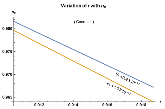
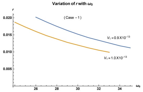
Case-1: Under the choice $n=1$, the potential (21) takes the form $V(\varphi )=V_0+V_1{\varphi }^2$, and thus the parameters of the theory under consideration (22) read as,

$$\begin{array}{c}\omega (\varphi )=\frac{{\omega }_0^2-3}{2},\frac{d\sigma }{d\varphi }=\frac{{\omega }_0}{\varphi },V_E=V_1+V_0{\varphi }^{-2},ϵ=\frac{4V_0^2}{{\omega }_0^2{(V_0+V_1{\varphi }^2)}^2},\hfill \\ \eta =\frac{8V_0}{{\omega }_0^2(V_0+V_1{\varphi }^2)},N=\frac{{\omega }_0^2}{4\sqrt{2}{V}_0}\left[V_1\left(\frac{{\varphi }_b^2}{2}-\frac{{\varphi }_e^2}{2}\right)+V_0(ln{\varphi }_b-ln{\varphi }_e)\right].\hfill \end{array}$$

(25)

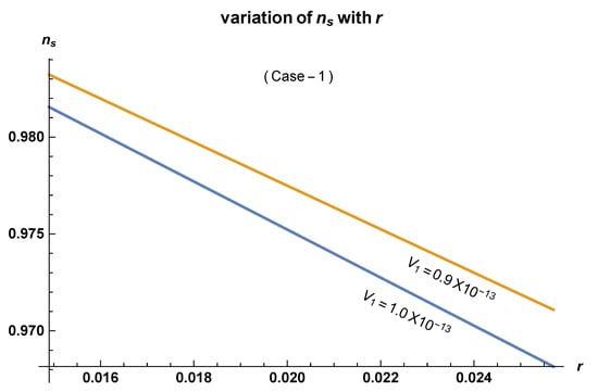
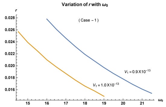
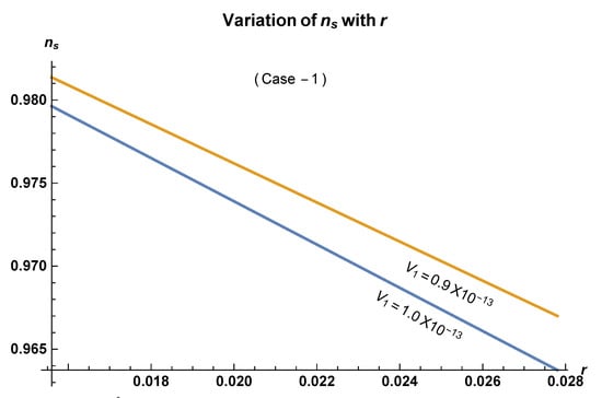
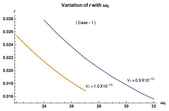
In view of the above forms of the slow roll parameters (25), we present Table 1 and Table 2, underneath, corresponding to two different values of the parameter $V_1>0$. The wonderful fit with the latest data sets released by Planck [40,41] is appreciable particularly because $0.968\approx n_s<0.982$, while $r<0.0278$. Further, the number of e-fold ($36\le N\le 62$) is sufficient to alleviate the horizon and flatness problems. Figure 1 and Figure 2 are the two plots r versus $n_s$ and r versus ${\omega }_0$ respectively, presented for visualization. For example, the figures clearly depict that the plot which represents data sets corresponding to Table 2 appears to be even better.

Table 1. $f(\varphi )=\varphi$, (case-1): ${\varphi }_b=2.0$. $V_0=-0.9\times {10}^{-13}{\mathrm{T}}^{-2},V_1=0.9\times {10}^{-13}{\mathrm{T}}^{-2}.$

${\mathit{\omega }}_0$	$|\mathit{\eta }|$	$\mathit{r}=16\mathit{ϵ}$	${\mathit{\varphi }}_{\mathit{e}}$	${\mathit{n}}_{\mathit{s}}$	N
16.0	0.010418	0.0278	1.060	0.9688	36
16.5	0.009795	0.0261	1.059	0.9706	38
17.0	0.009227	0.0246	1.057	0.9723	41
17.5	0.008707	0.0232	1.056	0.9739	43
18.0	0.008230	0.0219	1.054	0.9753	46
18.5	0.007792	0.0208	1.053	0.9766	48
19.0	0.007387	0.0197	1.051	0.9778	51
19.5	0.007013	0.0187	1.050	0.9790	54
20.0	0.006667	0.0178	1.049	0.9800	56
20.5	0.006345	0.0169	1.048	0.9810	59
21.0	0.006047	0.0161	1.047	0.9819	62

Table 2. $f(\varphi )=\varphi$, (case-1): ${\varphi }_b=2.0$. $V_0=-0.9\times {10}^{-13}{\mathrm{T}}^{-2},V_1=1.0\times {10}^{-13}{\mathrm{T}}^{-2}.$

${\mathit{\omega }}_0$	$|\mathit{\eta }|$	$\mathit{r}=16\mathit{ϵ}$	${\mathit{\varphi }}_{\mathit{e}}$	${\mathit{n}}_{\mathit{s}}$	N
14.5	0.011047	0.0257	1.012	0.9682	36
15.0	0.01032	0.0239	1.009	0.9703	38
15.5	0.009667	0.0225	1.008	0.9722	41
16.0	0.009072	0.0210	1.006	0.9739	43
16.5	0.008531	0.0198	1.005	0.9755	46
17.0	0.008037	0.0187	1.003	0.9769	49
17.5	0.007584	0.0176	1.001	0.9782	52
18.0	0.007168	0.0166	1.000	0.9794	55
18.5	0.006786	0.0158	0.9986	0.9805	59
19.0	0.006433	0.0149	0.9973	0.9815	62

Figure 1. $f=\varphi$, (case-1): Yellow ochre and blue colours represent Table 1 and Table 2 data, respectively.

Figure 2. $f=\varphi$, (case-1): Blue and yellow ochre colours represent Table 1 and Table 2 data, respectively.

One very interesting feature is that the above data sets remain unaltered even if the sign of $V_0$ and $V_1$ are interchanged. Note that, second derivative of the potential has to be positive, since it represents effective mass of the scalar field. In view of the forms of the potentials $V(\varphi )$ and $V_E(\sigma )$ presented in (21) and (22) the effective mass of the scalar fields $\varphi$ and $\sigma$ respectively are,

$$\frac{d^{2}V}{d{\varphi }^2}=2V_1;\frac{d^2{V}_E}{d{\sigma }^2}=6\frac{V_0}{{\varphi }^4}.$$

(26)

In our data set, we keep $V_1>0$, since $\varphi$ is the scalar field under consideration, while translation to $\sigma$ only amounts to handling the situation with considerable ease. However, as a matter of taste if one favours Einstein’s frame over Jordan’s frame, it is possible to revert the sign and keep $V_0>0$, without changing the data set.

As mentioned, at the end of inflation, the scalar field must oscillate rapidly so that particles are produced and the universe turns to the phase of: a hot thick soup of plasma, commonly called the ‘hot big-bang’. This phenomena is dubbed as graceful exit, which is required for the structure formation together with the formation of CMB. We therefore proceed to check if the present model admits graceful exit from inflation. Here, $V_E=V_1+\frac{V_0}{{\varphi }^2}$, and so one can express (19) as,

$$\begin{array}{c}\frac{3H^2}{V_1}=\frac{{\dot{\sigma }}^2}{2V_1}+\left(1+\frac{V_0}{V_1{\varphi }^2}\right).\hfill \end{array}$$

(27)

At large value of the scalar field, which in the present unit $\varphi >1$, we obtained slow-roll. However, as the scalar field falls below the Planck’s mass $M_p$, then the Hubble rate H also decreases, and once it falls below the effective mass $V_1$, i.e., $H\ll V_1$, then the above equation may be approximated to,

$${\dot{\sigma }}^2=2i^2\left(V_1+\frac{V_0}{{\varphi }^2}\right)⟶\dot{\varphi }=i\frac{\varphi }{{\omega }_0}\sqrt{2\left(V_1+\frac{V_0}{{\varphi }^2}\right)},$$

(28)

where, $\dot{\sigma }=\frac{{\omega }_0}{\varphi }\dot{\varphi }$, in view of (25). Thus, finally we get,

$$\varphi =\frac{1}{2V_1}\left[(1-V_0{V}_1)cos\left(\frac{\sqrt{2V_1}}{{\omega }_0}t\right)+i(1+V_0{V}_1)sin\left(\frac{\sqrt{2V_1}}{{\omega }_0}t\right)\right],$$

(29)

which is an oscillatory solution, and the field then oscillates many times over a Hubble time. This coherent oscillating field corresponds to a condensate of non-relativistic massive (inflaton) particles, which ensures graceful exit from the inflationary regime, driving a matter-dominated era at the end of inflation. There is a long standing debate regarding the physical frame. It appears that most of the people favour Einstein’s frame over Jordan’s frame (we have briefly discussed the issue in conclusion). In this regard, it is important to mention that since in view of (25) $\sigma ={\omega }_{0}ln\varphi$, therefore $\sigma$ executes oscillatory behaviour as well.

Case-2: Under the same situation $f(\varphi )=\varphi$, let us now consider, $V(\varphi )=V_1{\varphi }^2+V_0{\varphi }^4$, where instead of a constant term, we have added a quartic term in the potential. The expression for the Brans–Dicke parameter ($\omega (\varphi )$), the potential ($V_E$) in the Einstein frame, $\frac{d\sigma }{d\varphi }$, the slow-roll parameters $ϵ,\eta$ and the number of e-foldings N, may then be found in view of the Equation (24), respectively as,

$$\begin{array}{c}\omega (\varphi )=\frac{{\omega }_0^2-3}{2\varphi },\frac{d\sigma }{d\varphi }=\frac{{\omega }_0}{\varphi },V_E=V_1+V_0{\varphi }^2,ϵ=\frac{4V_0^2{\varphi }^4}{{\omega }_0^2{(V_1+V_0{\varphi }^2)}^2},\hfill \\ \eta =\frac{8V_0{\varphi }^2}{{\omega }_0^2(V_1+V_0{\varphi }^2)},N={\int }_{{\varphi }_e}^{{\varphi }_b}\frac{{\omega }_0^2(V_1+V_0{\varphi }^2)}{4\sqrt{2}{V}_0{\varphi }^3}d\varphi .\hfill \end{array}$$

(30)

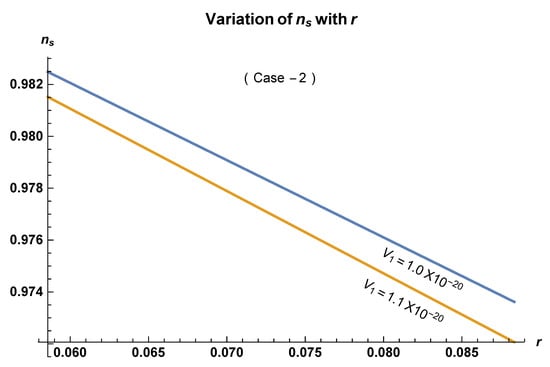
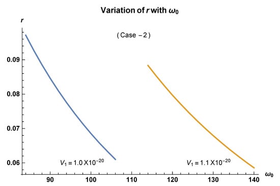
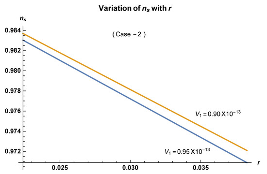
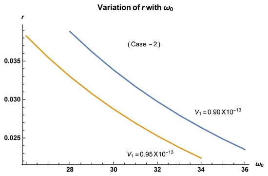
Although, the potential $V_E$ does not appear to attend a flat section, the smallness of the value of $\eta$ confirms that there indeed exists a flat section, admitting slow-roll. In fact, in the Einstein frame (17), this is just the case of a standard inflation field theory with quadratic potential. Following Table 3 and Table 4, for $V_1>0$, together with the associated plots $n_s$ versus r in Figure 3 and r versus ${\omega }_0$ in Figure 4 here again depict appreciably good fit with the recent released Planck’s data set, particularly because $0.97\le n_s\le 0.98$ while $r\le 0.098$. Figure 3 depicts that the data of Table 3 are somewhat better.

Table 3. $f(\varphi )=\varphi$, (case-2): ${\varphi }_b=1.2$, $V_0=-1.0\times {10}^{-20}{\mathrm{T}}^{-2};V_1=1.1\times {10}^{-20}{\mathrm{T}}^{-2}.$

${\mathit{\omega }}_0$	$|\mathit{\eta }|$	$\mathit{r}=16\mathit{ϵ}$	${\mathit{\varphi }}_{\mathit{e}}$	${\mathit{n}}_{\mathit{s}}$	N
114	0.002607	0.08834	1.0581	0.9721	38
116	0.002518	0.08532	1.0580	0.9730	39
118	0.002433	0.08245	1.0578	0.9739	41
120	0.002353	0.07972	1.0577	0.9748	42
122	0.002276	0.07713	1.0575	0.9756	44
124	0.002204	0.07466	1.0574	0.9764	45
126	0.002134	0.07231	1.0572	0.9772	46
128	0.002068	0.07007	1.0571	0.9779	48
130	0.002005	0.06793	1.0570	0.9785	49
132	0.001945	0.06589	1.0569	0.9792	51
134	0.001887	0.06393	1.0567	0.9798	53
136	0.001832	0.06207	1.0566	0.9804	54
138	0.001780	0.06028	1.0565	0.9810	56
140	0.001729	0.05857	1.0564	0.9815	57

Table 4. $f(\varphi )=\varphi$, (case-2): ${\varphi }_b=1.2$, $V_0=-1.0\times {10}^{-20}{\mathrm{T}}^{-2};V_1=1.0\times {10}^{-20}{\mathrm{T}}^{-2}.$

${\mathit{\omega }}_0$	$|\mathit{\eta }|$	$\mathit{r}=16\mathit{ϵ}$	${\mathit{\varphi }}_{\mathit{e}}$	${\mathit{n}}_{\mathit{s}}$	N
84	0.003711	0.09715	1.0121	0.9710	36
86	0.003540	0.09268	1.0118	0.9723	38
88	0.003381	0.08852	1.0115	0.9736	40
90	0.003232	0.08463	1.0113	0.9747	42
92	0.003093	0.08099	1.0110	0.9758	44
94	0.002963	0.07758	1.0108	0.9768	46
96	0.002841	0.07438	1.0105	0.9778	47
98	0.002726	0.07138	1.0103	0.9787	49
100	0.002618	0.06855	1.0101	0.9795	51
102	0.002517	0.06589	1.0099	0.9803	54
104	0.002421	0.0634	1.0097	0.9810	56
106	0.002330	0.06101	1.0096	0.9818	58

Figure 3. $f=\varphi$. Yellow ochre and blue colours represent Table 3 and Table 4 respectively.

Figure 4. $f=\varphi$. Yellow ochre and blue colours represent Table 3 and Table 4 respectively, unlike previous cases.

As before here again we test if the model associated with a different potential admits graceful exit. Here $V_E=(V_1+V_0{\varphi }^2)$, and so from (19) one obtains,

$$\begin{array}{c}\frac{3H^2}{V_1}=\frac{{\dot{\sigma }}^2}{2V_1}+\left(1+\frac{V_0}{V_1}{\varphi }^2\right)\hfill \end{array}$$

(31)

As the Hubble rate $H\ll V_1$, the above equation can be approximated to, ${\dot{\sigma }}^2=2i^2(V_1+V_0{\varphi }^2)$, yielding $\dot{\varphi }=i\frac{\varphi }{{\omega }_0}\sqrt{2(V_1+V_0{\varphi }^2)}$, where, $\dot{\sigma }=\dot{\varphi }\frac{{\omega }_0}{\varphi }$. Finally we get,

$$\varphi =\frac{2V_1\left[(1-V_0{V}_1)cos\left(\frac{\sqrt{2V_1}}{{\omega }_0}t\right)+i(1+V_0{V}_1)sin\left(\frac{\sqrt{2V_1}}{{\omega }_0}t\right)\right]}{1+V_0^2{V}_1^2-2V_0{V}_{1}cos\left(\frac{2\sqrt{2V_1}}{{\omega }_0}t\right)}.$$

(32)

The oscillatory behaviour of the scalar field clearly ensures graceful exit from inflationary regime, as already discussed, and in view of (30) $\sigma$ also executes oscillatory behaviour.

3.1.2. $n=\frac{3}{2},f(\varphi )={\varphi }^{\frac{3}{2}}$

Case-1: Under the choice $n=\frac{3}{2}$, $f(\varphi )={\varphi }^{\frac{3}{2}}$, and the potential (21) takes the cubic form, $V(\varphi )=V_0+V_1{\varphi }^3$. Thus the expressions for the parameters of the theory under consideration along with the slow-roll parameters (22) are,

$$\begin{array}{c}\omega (\varphi )=\frac{4{\omega }_0^2-27\varphi }{8\sqrt{\varphi }},\frac{d\sigma }{d\varphi }=\frac{{\omega }_0}{{\varphi }^{\frac{3}{2}}};V_E=V_1+V_0{\varphi }^{-3},ϵ=\frac{9V_0^2\varphi }{{\omega }_0^2{(V_0+V_1{\varphi }^3)}^2},\hfill \\ \eta =\frac{15V_0\varphi }{{\omega }_0^2(V_0+V_1{\varphi }^3)},N=\frac{{\omega }_0^2}{6\sqrt{2}{V}_0}\left[V_0\left(\frac{1}{{\varphi }_e}-\frac{1}{{\varphi }_b}\right)+\frac{V_1}{2}({\varphi }_b^2-{\varphi }_e^2)\right].\hfill \end{array}$$

(33)

As before, we present two sets of data in Table 5 and Table 6, for two different values of $V_1>0$. Figure 5 and Figure 6 depict the variations of the spectral index $n_s$ with the scalar-tensor ratio r and the scalar-tensor ratio r with the Brans–Dicke parameter ${\omega }_0$ respectively. Here again we observe that $r\le 0.0278$, and $0.96<n_s<0.9815$, which are very much within the stipulated observational range [40,41], while number of e-folding N is sufficient to remove the flatness and the horizon problems.

Table 5. $f(\varphi )={\varphi }^{\frac{3}{2}}$, (case-1): ${\varphi }_b=1.7$, $V_0=-0.9\times {10}^{-13}{\mathrm{T}}^{-2},V_1=0.9\times {10}^{-13}{\mathrm{T}}^{-2}.$

${\mathit{\omega }}_0$	$|\mathit{\eta }|$	$\mathit{r}=16\mathit{ϵ}$	${\mathit{\varphi }}_{\mathit{e}}$	${\mathit{n}}_{\mathit{s}}$	N
24	0.011314	0.0278	1.0408	0.9670	36
25	0.010427	0.0256	1.0392	0.9696	39
26	0.009640	0.0237	1.0377	0.9719	42
27	0.008939	0.0219	1.0364	0.9739	46
28	0.008312	0.0204	1.0351	0.9757	49
29	0.007749	0.0190	1.0339	0.9773	52
30	0.007241	0.0178	1.0328	0.9788	56
31	0.006781	0.0166	1.0318	0.9802	60
32	0.006364	0.0156	1.0308	0.9814	64

Table 6. $f(\varphi )={\varphi }^{\frac{3}{2}}$, (case-1): ${\varphi }_b=1.7$, $V_0=-0.9\times {10}^{-13}{\mathrm{T}}^{-2},V_1=1.0\times {10}^{-13}{\mathrm{T}}^{-2}.$

${\mathit{\omega }}_0$	$|\mathit{\eta }|$	$\mathit{r}=16\mathit{ϵ}$	${\mathit{\varphi }}_{\mathit{e}}$	${\mathit{n}}_{\mathit{s}}$	N
22.0	0.011816	0.0254	1.0076	0.9668	36
22.5	0.011217	0.0243	1.0067	0.9683	38
23.0	0.010811	0.0233	1.0059	0.9697	39
23.5	0.010356	0.0223	1.0050	0.9709	41
24.0	0.009928	0.0214	1.0042	0.9721	43
24.5	0.009528	0.0205	1.0034	0.9733	45
25.0	0.009150	0.0197	1.0027	0.9743	47
25.5	0.008795	0.0189	1.0019	0.9753	48
26.0	0.008460	0.0182	1.0013	0.9762	50
26.5	0.008143	0.0175	1.0006	0.9771	52
27.0	0.007845	0.0169	1.000	0.9780	54

Figure 5. $f(\varphi )={\varphi }^{\frac{3}{2}}$. Yellow ochre and blue colours represent Table 5 and Table 6 respectively.

Figure 6. $f(\varphi )={\varphi }^{\frac{3}{2}}$. Blue and yellow ochre colours represent Table 5 and Table 6 respectively.

To check the behaviour of the scalar field, we proceed as before, and find,

$$\frac{3H^2}{V_1}=\frac{{\omega }_0^2{\dot{\varphi }}^2}{2V_1{\varphi }^3}+\frac{V_0}{V_1{\varphi }^3}+1⟹{\dot{\varphi }}^2=-2\frac{(V_0+V_1{\varphi }^3)}{{\omega }_0^2},$$

(34)

under suitable approximation, as the Hubble rate $H\ll V_1$, and using the relation $\dot{\sigma }={\omega }_0\frac{\dot{\varphi }}{{\varphi }^{\frac{3}{2}}}$, in view of (33). The solution reads as,

$$\begin{array}{c}\hfill \begin{array}{cc}\hfill \varphi (t)=& \mathrm{InverseFunction}[\frac{2i}{\sqrt[4]{3}\sqrt[3]{V_1}\sqrt{V_0-\#1^3{V}_1}}\mathrm{Elliptic}\mathrm{F}\left[{\mathrm{Sin}}^{-1}\left(\frac{1}{\sqrt[4]{3}}\sqrt{-{(-1)}^{\frac{5}{6}}-i\#1\sqrt[3]{\frac{V_1}{V_0}}}\right),\sqrt[3]{-1}\right]\hfill \\ \hfill & \left.\sqrt[3]{V_0}\sqrt{{(-1)}^{5/6}\left(\#1\sqrt[3]{\frac{V_1}{V_0}}-1\right)}\sqrt{\#1^2\sqrt[3]{\frac{V_1^2}{V_0^2}}+\#1\sqrt[3]{\frac{V_1}{V_0}}+1}\&\right]\left[c_1-t\right].\hfill \end{array}\end{array}$$

(35)

In the above the hash tag ($\#n$) denotes nth argument of a pure function, and $c_1$ is a constant. Although, the solution is not obtainable in closed form, rather is a complicated inverse elliptic function, nevertheless its oscillatory behaviour is quite apparent, and $\sigma =-2\frac{{\omega }_0}{\sqrt{\varphi }}$ also oscillates as well.

Case-2: Under the choice $n=\frac{3}{2}$, $f(\varphi )={\varphi }^{\frac{3}{2}}$, and taking the potential in the form, $V(\varphi )=V_1{\varphi }^3+V_0\varphi$, the expressions for the parameters of the theory under consideration along with the slow-roll parameters (24) are,

$$\begin{array}{c}\omega (\varphi )=\frac{4{\omega }_0^2-27\varphi }{8\sqrt{\varphi }},\frac{d\sigma }{d\varphi }=\frac{{\omega }_0}{{\varphi }^{\frac{3}{2}}};V_E=V_1+\frac{V_0}{{\varphi }^2},ϵ=\frac{4V_0^2\varphi }{{\omega }_0^2{(V_0+V_1{\varphi }^2)}^2},\hfill \\ \eta =\frac{6V_0\varphi }{{\omega }_0^2(V_0+V_1{\varphi }^2)},N=\frac{{\omega }_0^2}{4\sqrt{2}{V}_0}\left[V_0\left(\frac{1}{{\varphi }_e}-\frac{1}{{\varphi }_b}\right)+V_1({\varphi }_b-{\varphi }_e)\right].\hfill \end{array}$$

(36)

We present two sets of data in Table 7 and Table 8 underneath, for two different values of $V_1>0$. Figure 7 and Figure 8 depict the variations of the spectral index $n_s$ with the scalar-tensor ratio r, and the scalar-tensor ratio r with the Brans–Dicke parameter ${\omega }_0$, respectively. Here also we observe that $r\le 0.039$, and $0.971<n_s<0.983$, which are again in excellent agreement of Planck’s data [40,41], while the number of e-folding N is also sufficient to remove the flatness and the horizon problems.

Table 7. $f(\varphi )={\varphi }^{\frac{3}{2}}$, (case-2): ${\varphi }_b=1.7$, $V_0=-0.9\times {10}^{-13}{\mathrm{T}}^{-2},V_1=0.90\times {10}^{-13}{\mathrm{T}}^{-2}.$

${\mathit{\omega }}_0$	$|\mathit{\eta }|$	$\mathit{r}=16\mathit{ϵ}$	${\mathit{\varphi }}_{\mathit{e}}$	${\mathit{n}}_{\mathit{s}}$	N
28	0.006884	0.03885	1.0357	0.9717	40
29	0.006417	0.03623	1.0345	0.9736	43
30	0.005996	0.03384	1.0333	0.9753	46
31	0.005616	0.03169	1.0323	0.9769	49
32	0.005270	0.02974	1.0313	0.9783	52
33	0.004956	0.02797	1.0303	0.9796	55
34	0.004669	0.02635	1.0294	0.9808	59
35	0.004406	0.02486	1.0286	0.9819	62
36	0.004164	0.02350	1.0278	0.9829	66

Table 8. $f(\varphi )={\varphi }^{\frac{3}{2}}$, (case-2): ${\varphi }_b=1.7$, $V_0=-0.9\times {10}^{-13}{\mathrm{T}}^{-2},V_1=0.95\times {10}^{-13}{\mathrm{T}}^{-2}.$

${\mathit{\omega }}_0$	$|\mathit{\eta }|$	$\mathit{r}=16\mathit{ϵ}$	${\mathit{\varphi }}_{\mathit{e}}$	${\mathit{n}}_{\mathit{s}}$	N
26	0.007358	0.03828	1.0103	0.9709	39
27	0.006823	0.03549	1.0089	0.9730	42
28	0.006345	0.03300	1.0076	0.9749	45
29	0.005915	0.03077	1.0064	0.9766	48
30	0.005527	0.02875	1.0053	0.9782	52
31	0.005176	0.02693	1.0043	0.9796	55
32	0.004858	0.02527	1.0033	0.9808	59
33	0.004568	0.02376	1.0024	0.9820	63
34	0.004303	0.02238	1.0016	0.9830	67

Figure 7. $f(\varphi )={\varphi }^{\frac{3}{2}}$. Yellow ochre and blue colours represent Table 7 and Table 8 respectively.

Figure 8. $f(\varphi )={\varphi }^{\frac{3}{2}}$. Blue and yellow ochre colours represent Table 7 and Table 8 respectively.

In order to study the behaviour of the scalar field at the end of inflation, we start with the Einstein frame potential as before, $V_E=(V_1+\frac{V_0}{{\varphi }^2})$, and express the field Equation (19) as,

$$\begin{array}{c}\frac{3H^2}{V_1}=\frac{{\dot{\sigma }}^2}{2V_1}+\left(1+\frac{V_0}{V_1{\varphi }^2}\right)\hfill \end{array}$$

(37)

As the Hubble rate falls, and $H\ll V_1$, the above equation may be approximated to, ${\dot{\sigma }}^2=2i^2(V_1+\frac{V_0}{{\varphi }^2})$, which in terms of the scalar field $\varphi$ reads as,

$${\dot{\varphi }}^2+\frac{2}{{\omega }_0^2}\left(V_0+V_1{\varphi }^2\right)\varphi =0.$$

(38)

The above equation when solved, is found to execute oscillatory behaviour as before, along with $\sigma =-2\frac{{\omega }_0}{\sqrt{\varphi }}$, as well.

$$\begin{array}{c}\hfill \varphi (t)=\mathrm{InverseFunction}\left[\frac{2i\#1^{3/2}\sqrt{\frac{V_0}{\#1^2{V}_1}+1}\mathrm{Elliptic}\mathrm{F}\left(\left.i{sinh}^{-1}\left(\frac{\sqrt{-\frac{i\sqrt{V_0}}{\sqrt{V_1}}}}{\sqrt{\#1}}\right)\right|-1\right)}{\sqrt{-\frac{i\sqrt{V_0}}{\sqrt{V_1}}}\sqrt{-\#1\left(\#1^2{V}_1+V_0\right)}}\&\right]\left[c_1+\frac{\sqrt{2}t}{{\omega }_0}\right],\end{array}$$

(39)

Case-3: Cubic potentials with additive term have important consequence. For example, a potential in the form $V=\frac{1}{2}m{\omega }^2{x}^2-\frac{1}{3}b{x}^3$ can be used to model decay of metastable states [55], and it also describes the global flow [56]. Further, the tunnelling rate in real time in the semiclassical limit may be found for arbitrary energy levels, while its ground state agrees well with the result found by the instanton method [57]. It is therefore worth to continue the present study in view of such an additive form in the cubic potential.

Under the choice $n=\frac{3}{2}$, $f(\varphi )={\varphi }^{\frac{3}{2}}$, and taking the potential as cubic form added with a quadratic term, i.e., $V(\varphi )=V_1{\varphi }^3+V_0{\varphi }^2$, the expressions for the parameters of the theory under consideration along with the slow-roll parameters (24) are,

$$\begin{array}{c}\omega (\varphi )=\frac{4{\omega }_0^2-27\varphi }{8\sqrt{\varphi }},\frac{d\sigma }{d\varphi }=\frac{{\omega }_0}{{\varphi }^{\frac{3}{2}}};V_E=V_1+\frac{V_0}{\varphi },ϵ=\frac{V_0^2\varphi }{{\omega }_0^2{(V_0+V_1\varphi )}^2},\hfill \\ \eta =\frac{V_0\varphi }{{\omega }_0^2(V_0+V_1\varphi )},N=\frac{{\omega }_0^2}{2\sqrt{2}{V}_0}\left[V_0\left(\frac{1}{{\varphi }_e}-\frac{1}{{\varphi }_b}\right)+V_{1}ln({\varphi }_b-{\varphi }_e)\right].\hfill \end{array}$$

(40)

We present two sets of data in Table 9 and Table 10 underneath, for two different values of $V_1>0$. Figure 9 and Figure 10 depict the variations of the spectral index $n_s$ with the scalar-tensor ratio r and the scalar-tensor ratio r with the Brans–Dicke parameter ${\omega }_0$ respectively. Here also we observe that $r\le 0.062$, and $0.973<n_s<0.983$, which are again in excellent agreement of Planck’s data [40,41], while the number of e-folding N is also sufficient to remove the flatness and the horizon problems. It is interesting to note that the variation $n_s$ with r for the two sets of data almost overlap in Figure 9.

Table 9. $f(\varphi )={\varphi }^{\frac{3}{2}}$, (case-3): ${\varphi }_b=1.7$, $V_0=-0.9\times {10}^{-13}{\mathrm{T}}^{-2},V_1=0.9\times {10}^{-13}{\mathrm{T}}^{-2}.$

${\mathit{\omega }}_0$	$|\mathit{\eta }|$	$\mathit{r}=16\mathit{ϵ}$	${\mathit{\varphi }}_{\mathit{e}}$	${\mathit{n}}_{\mathit{s}}$	N
30	0.00270	0.0617	1.0339	0.9715	38
31	0.00253	0.0578	1.0328	0.9733	40
32	0.00237	0.0542	1.0317	0.9749	43
33	0.00223	0.0509	1.0308	0.9764	46
34	0.00210	0.0480	1.0299	0.9778	48
35	0.00198	0.0453	1.0290	0.9790	51
36	0.00187	0.0428	1.0282	0.9802	54
37	0.00177	0.0405	1.0273	0.9812	57
38	0.00168	0.0384	1.0267	0.9822	61

Table 10. $f(\varphi )={\varphi }^{\frac{3}{2}}$, (case-3): ${\varphi }_b=1.7$, $V_0=-0.9\times {10}^{-13}{\mathrm{T}}^{-2},V_1=0.92\times {10}^{-13}{\mathrm{T}}^{-2}.$

${\mathit{\omega }}_0$	$|\mathit{\eta }|$	$\mathit{r}=16\mathit{ϵ}$	${\mathit{\varphi }}_{\mathit{e}}$	${\mathit{n}}_{\mathit{s}}$	N
29	0.00274	0.0594	1.0122	0.9723	39
30	0.00256	0.0555	1.0110	0.9741	41
31	0.00240	0.0520	1.0097	0.9757	44
32	0.00225	0.0488	1.0090	0.9772	47
33	0.00212	0.0459	1.0080	0.9786	50
34	0.00199	0.0432	1.0071	0.9798	53
35	0.00188	0.0408	1.0063	0.9809	56
36	0.00178	0.0386	1.0055	0.9820	60
37	0.00168	0.0365	1.0048	0.9829	63

Figure 9. $f(\varphi )={\varphi }^{\frac{3}{2}}$. Yellow ochre and blue colours represent Table 9 and Table 10 respectively.

Figure 10. $f(\varphi )={\varphi }^{\frac{3}{2}}$. Blue and yellow ochre colours represent Table 9 and Table 10 respectively.

In order to study the behaviour of the scalar field at the end of inflation, we start with the Einstein frame potential as before, $V_E=(V_1+\frac{V_0}{\varphi })$, and express the field Equation (19) as,

$$\begin{array}{c}\frac{3H^2}{V_1}=\frac{{\dot{\sigma }}^2}{2V_1}+\left(1+\frac{V_0}{V_1\varphi }\right)\hfill \end{array}$$

(41)

As the Hubble rate falls, and $H\ll V_1$, the above equation may be approximated to, ${\dot{\sigma }}^2=2i^2(V_1+\frac{V_0}{\varphi })$, which in terms of the scalar field $\varphi$ reads as,

$${\dot{\varphi }}^2+\frac{2}{{\omega }_0^2}\left(V_0+V_1\varphi \right){\varphi }^2=0.$$

(42)

The above equation may be solved to find

$$\varphi =\frac{V_0}{V_1}\left[-1-tan{\left\{\frac{\sqrt{V_0}}{2}\left(c_1+\frac{\sqrt{2}}{{\omega }_0}t\right)\right\}}^2\right],$$

(43)

which unfortunately is not oscillatory. Perhaps, due to the asymmetry of the potential, the oscillatory behaviour of the scalar field with an additive quadratic term is not exhibited.

3.1.3. $n=2,f(\varphi )={\varphi }^2$

Case-1: Under the choice $n=2$, $f(\varphi )={\varphi }^2$, and the potential (21) is now chosen as $V(\varphi )=V_0+V_1{\varphi }^4$. Therefore the Brans–Dicke parameter and the Einstein frame potential, together with the slow-roll parameters (22), take the following forms,

$$\begin{array}{c}\omega (\varphi )=\frac{{\omega }_0^2-12{\varphi }^2}{2\varphi },\frac{d\sigma }{d\varphi }=\frac{{\omega }_0}{{\varphi }^2};V_E=V_1+V_0{\varphi }^{-4},ϵ=\frac{16V_0^2{\varphi }^2}{{\omega }_0^2{(V_0+V_1{\varphi }^4)}^2},\hfill \\ \eta =\frac{24V_0{\varphi }^2}{{\omega }_0^2(V_0+V_1{\varphi }^4)},N=\frac{{\omega }_0^2}{8\sqrt{2}{V}_0}\left[\frac{V_0}{2}\left(\frac{1}{{\varphi }_e^2}-\frac{1}{{\varphi }_b^2}\right)+\frac{V_1}{2}({\varphi }_b^2-{\varphi }_e^2)\right].\hfill \end{array}$$

(44)

It is quite transparent that for large value of the scalar field $\varphi$, a flat Einstein’s frame potential is realizable here too. As before, we take two sets of data corresponding to two different values of $V_1>0$, and tabulate the parametric values in Table 11 and Table 12. One can see that the scalar tensor ratio $r\le 0.0202$, and the spectral index lies between $0.9645\le n_s\le 0.9809$, which are in excellent agreement with Planck’s data [40,41]. Further number of e-folding N is also sufficient to alleviate the flatness and the horizon problems. The $n_s$ versus r and r versus ${\omega }_0$ plots are presented in Figure 11 and Figure 12, as well.

Table 11. $f(\varphi )={\varphi }^2$, (case-1): ${\varphi }_b=1.7$, $V_0=-0.9\times {10}^{-13}{\mathrm{T}}^{-2},V_1=0.9\times {10}^{-13}{\mathrm{T}}^{-2}.$

${\mathit{\omega }}_0$	$|\mathit{\eta }|$	$\mathit{r}=16\mathit{ϵ}$	${\mathit{\varphi }}_{\mathit{e}}$	${\mathit{n}}_{\mathit{s}}$	N
26	0.013956	0.0202	1.0377	0.9645	37
27	0.012941	0.0188	1.0364	0.9671	39
28	0.012033	0.0175	1.0351	0.9694	42
29	0.01122	0.0163	1.0339	0.9715	45
30	0.010482	0.0152	1.0328	0.9733	49
31	0.009817	0.0142	1.0317	0.9750	52
32	0.009213	0.0134	1.0308	0.9766	56
33	0.008663	0.0126	1.0298	0.9780	59
34	0.008161	0.0118	1.0289	0.9792	63
35	0.007701	0.0112	1.0282	0.9804	67

Table 12. $f(\varphi )={\varphi }^2$, (case-1): ${\varphi }_b=1.7$. $V_0=-0.9\times {10}^{-13}{\mathrm{T}}^{-2},V_1=1.0\times {10}^{-13}{\mathrm{T}}^{-2}.$

${\mathit{\omega }}_0$	$|\mathit{\eta }|$	$\mathit{r}=16\mathit{ϵ}$	${\mathit{\varphi }}_{\mathit{e}}$	${\mathit{n}}_{\mathit{s}}$	N
24	0.014543	0.0187	1.0127	0.9639	37
25	0.013403	0.0173	1.0112	0.9667	40
26	0.012392	0.0160	1.0098	0.9692	43
27	0.011491	0.0148	1.0085	0.9714	46
28	0.010685	0.0138	1.0073	0.9735	50
29	0.00996	0.0128	1.0062	0.9753	54
30	0.00931	0.0120	1.0051	0.9769	57
31	0.008717	0.0112	1.0041	0.9784	61
32	0.008180	0.0105	1.0032	0.9797	65
33	0.007692	0.0099	1.0023	0.9809	69

Figure 11. $f(\varphi )={\varphi }^2$. Blue and yellow ochre colours represent Table 11 and Table 12 respectively.

Figure 12. $f(\varphi )={\varphi }^2$. Blue and yellow ochre colours represent Table 11 and Table 12 respectively.

Equation (19) now reads as,

$$3H^2=\frac{1}{2}{\dot{\sigma }}^2+V_1+\frac{V_0}{{\varphi }^4},$$

(45)

which, as H falls below $V_1$, i.e., $H\ll V_1$, may be approximated to, $\frac{1}{2}{\dot{\sigma }}^2+\frac{V_0}{{\varphi }^4}+V_1=0$. In terms of the scalar field $\varphi$ it is expressed as ${\dot{\varphi }}^2+\frac{2}{{\omega }_0^2}\left(V_1{\varphi }^4+V_0\right)=0$, since, $\dot{\sigma }={\omega }_0\frac{\dot{\varphi }}{{\varphi }^2}$, in view of (44). The solution is exhibited either as,

$$\varphi (t)=-\frac{{(-1)}^{3/4}\sqrt[4]{V_0}\mathrm{JacobiSN}\left(\left.c_1\sqrt[4]{-V_0{V}_1}\left(1+i\frac{\sqrt{2}}{{\omega }_0}t\right)\right|-1\right)}{\sqrt[4]{V_1}},$$

(46)

(where JacobiSN is a meromorphic function in both arguments, which for certain special arguments may automatically be evaluated to exact values. In any case, under numerical simulation the above solution is found to exhibit oscillatory behaviour of the scalar field $\varphi$), or as inverse elliptic function as before,

$$\begin{array}{c}\hfill \varphi (t)=\mathrm{InverseFunction}\left[-\frac{i\sqrt{\frac{\#1^4{V}_1}{V_0}+1}\mathrm{Elliptic}F\left(\left.i{sinh}^{-1}\left(\#1\sqrt{-\frac{i\sqrt{V_1}}{\sqrt{V_0}}}\right)\right|-1\right)}{\sqrt{-\frac{i\sqrt{V_1}}{\sqrt{V_0}}}\sqrt{\#1^4\left(-V_1\right)-V_0}}\&\right]\left[c_1+\frac{\sqrt{2}t}{{\omega }_0}\right],\end{array}$$

(47)

It is also clear that $\sigma =-\frac{{\omega }_0}{\varphi }$ oscillates as well, and the universe transits from inflationary regime to the matter dominated era.

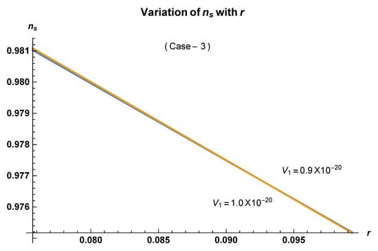
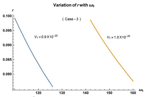
Case-2: Here, for $f(\varphi )={\varphi }^2$, we consider the potential in the form, $V=V_1{\varphi }^4+V_0{\varphi }^2$, i.e., instead of a constant additive term, we consider $V_0{\varphi }^2$ in addition. This case was earlier studied in [37]. However, as already mentioned, over the years, Planck’s data put up tighter constraints on inflationary parameters, and so it is quite reasonable to check if this form of potential passes the said constraints [40,41]. One can now find the expression for the Brans–Dicke parameter $\omega (\varphi )$, the potential $V_E$ in the Einstein frame, $\frac{d\sigma }{d\varphi }$, the slow-roll parameters $ϵ,\eta$ and the number of e-folding N, in view of the Equations (24), respectively as,

$$\begin{array}{c}\omega (\varphi )=\frac{{\omega }_0^2-12{\varphi }^2}{2\varphi },\frac{d\sigma }{d\varphi }=\frac{{\omega }_0}{{\varphi }^2};V_E=V_1+V_0{\varphi }^{-2},ϵ=\frac{4V_0^2{\varphi }^2}{{\omega }_0^2{(V_1{\varphi }^2+V_0)}^2},\hfill \\ \eta =\frac{4V_0{\varphi }^2}{{\omega }_0^2(V_1{\varphi }^2+V_0)},N=\frac{{\omega }_0^2}{4\sqrt{2}{V}_0}\left[V_{1}ln({\varphi }_b-{\varphi }_e)-\frac{V_0}{2}\left(\frac{1}{{\varphi }_b^2}-\frac{1}{{\varphi }_e^2}\right)\right].\hfill \end{array}$$

(48)

Note that the Einstein frame potential now takes the same form as in case-1 for $n=1$, and a flat section of the potential is still realizable at large value of the scalar field $\varphi$. We present two Table 13 and Table 14, as before for different values of $V_1>0$. The scalar to tensor ratio $r\le 0.0636$ and the spectral index $0.9715\le n_s\le 0.9831$ lie very much within the Planck’s data, while the number of e-folding N is again sufficient to alleviate the horizon and flatness problems. The Figure 13 and Figure 14 represent $n_s$ versus r and r versus ${\omega }_0$ respectively. In view of the plots, the data for Table 14, here appears to be even better.

Table 13. $f(\varphi )={\varphi }^2$, (case-2): ${\varphi }_b=1.26$. $V_0=-1.0\times {10}^{-20}{\mathrm{T}}^{-2};V_1=1.0\times {10}^{-20}{\mathrm{T}}^{-2}$.

${\mathit{\omega }}_0$	$|\mathit{\eta }|$	$\mathit{r}=16\mathit{ϵ}$	${\mathit{\varphi }}_{\mathit{e}}$	${\mathit{n}}_{\mathit{s}}$	N
68	0.002337	0.0636	1.0148	0.9715	37
70	0.002206	0.0601	1.0144	0.9731	40
72	0.002085	0.0568	1.0140	0.9745	42
74	0.001974	0.0537	1.0136	0.9759	44
76	0.001871	0.0509	1.0132	0.9772	47
78	0.001776	0.0484	1.0129	0.9783	49
80	0.001689	0.0460	1.0126	0.9793	52
82	0.001607	0.0438	1.0122	0.9804	55
84	0.001532	0.0417	1.0119	0.9813	57
86	0.001461	0.0398	1.0117	0.9821	60
88	0.001396	0.0380	1.0114	0.9830	63

Table 14. $f(\varphi )={\varphi }^2$, (case-2.): ${\varphi }_b=1.26.$$V_0=-1.0\times {10}^{-20}{\mathrm{T}}^{-2};V_1=1.1\times {10}^{-20}{\mathrm{T}}^{-2}$.

${\mathit{\omega }}_0$	$|\mathit{\eta }|$	$\mathit{r}=16\mathit{ϵ}$	${\mathit{\varphi }}_{\mathit{e}}$	${\mathit{n}}_{\mathit{s}}$	N
60	0.002363	0.0507	1.0656	0.9762	38
61	0.002287	0.0490	1.0653	0.9770	39
62	0.002213	0.0475	1.0650	0.9778	40
63	0.002144	0.0460	1.0648	0.9785	41
64	0.002078	0.0445	1.0646	0.9792	43
65	0.002014	0.0432	1.0643	0.9798	44
66	0.001953	0.0419	1.0641	0.9804	46
67	0.001895	0.0406	1.0638	0.9810	47
68	0.001840	0.0394	1.0636	0.9815	49
69	0.001787	0.0383	1.0634	0.9821	50
70	0.001737	0.0372	1.0632	0.9826	51
71	0.001688	0.0362	1.0630	0.9831	53

Figure 13. $f(\varphi )={\varphi }^2$. Yellow ochre and blue colours represent Table 13 and Table 14 respectively.

Figure 14. $f(\varphi )={\varphi }^2$. Blue and yellow ochre colours represent Table 13 and Table 14 respectively.

To check if the scalar field executes oscillatory behaviour at the end of inflation, we note that here $V_E=V_1+\frac{V_0}{{\varphi }^2}$. So in view of Equation (19) one obtains,

$$\begin{array}{c}\frac{3H^2}{V_1}=\frac{{\dot{\sigma }}^2}{2V_1}+\left(1+\frac{V_0}{V_1{\varphi }^2}\right)\hfill \end{array}$$

(49)

As, H falls below $V_1$, and $H\ll V_1$, the above equation can be approximated to, ${\dot{\sigma }}^2=2i^2\left(V_1+\frac{V_0}{{\varphi }^2}\right)$, yielding, $\dot{\varphi }=i\frac{\varphi }{{\omega }_0}\sqrt{2(V_0+V_1{\varphi }^2})$, where, $\dot{\sigma }={\omega }_0\frac{\dot{\varphi }}{{\varphi }^2}$. Thus, we obtain,

$$\frac{\varphi }{\left({\sqrt{V}}_0+\sqrt{(V_0+V_1{\varphi }^2)}\right)}={\sqrt{V}}_0{e}^{i\frac{\sqrt{2V_0}}{{\omega }_0}t}.$$

(50)

It is also possible to solve for $\varphi$ and express it in the following form,

$$\begin{array}{c}\varphi (t)=\frac{\sqrt{-\beta (t)+\sqrt{\beta {(t)}^2-4\alpha (t)\gamma (t)}}}{\sqrt{2\alpha (t)}},\hfill \\ \mathrm{where},\alpha (t)=1-V_0{V}_1{e}^{i2\frac{\sqrt{2V_0}}{{\omega }_0}t},\beta (t)=-4V_0^3{V}_1{e}^{i4\frac{\sqrt{2V_0}}{{\omega }_0}t},\gamma (t)=-4V_0^4{e}^{i4\frac{\sqrt{2V_0}}{{\omega }_0}t}.\hfill \end{array}$$

(51)

It is now quite apparent that the scalar field $\varphi (t)$ executes oscillatory behaviour and therefore graceful exit from inflation is realizable. Since in view of (48) $\sigma =-\frac{{\omega }_0}{\varphi }$, therefore $\sigma$ also executes oscillatory behaviour.

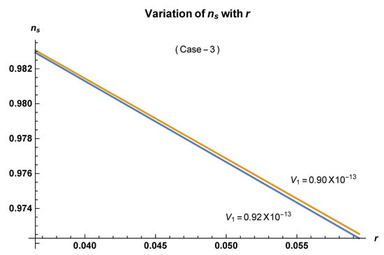
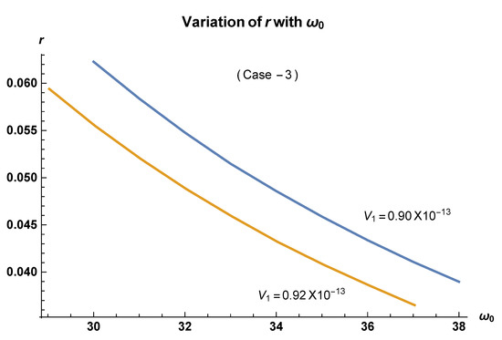
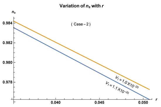
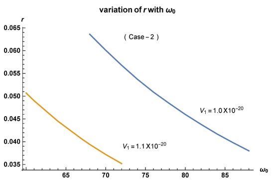
Case-3: We consider yet another case for $n=2$, i.e., taking $f(\varphi )={\varphi }^2$, with the potential $V(\varphi )$ being represented by two additional terms apart from ${\varphi }^4$, as it should be, to make it a perfect square: $V(\varphi )={(\sqrt{V_1}{\varphi }^2-\sqrt{V_0}\varphi )}^2=V_1{\varphi }^4+V_0{\varphi }^2-2\sqrt{V_0{V}_1}{\varphi }^3$. As before, one can now find the expression for the Brans–Dicke parameter $\omega (\varphi )$, the potential $V_E$ in the Einstein frame, $\frac{d\sigma }{d\varphi }$, the slow-roll parameters $ϵ,\eta$ and the number of e-foldings N, in view of the Equations (14), (18) and (20) respectively as,

$$\begin{array}{c}\omega (\varphi )=\frac{{\omega }_0^2-12{\varphi }^2}{2\varphi },\frac{d\sigma }{d\varphi }=\frac{{\omega }_0}{{\varphi }^2};V_E=V_1-2\frac{\sqrt{V_0{V}_1}}{\varphi }+\frac{V_0}{{\varphi }^2},ϵ=\frac{4V_0^2{\varphi }^2}{{\omega }_0^2{(\sqrt{V_0{V}_1}\varphi -V_0)}^2},\hfill \\ \eta =\frac{4V_0^2{\varphi }^2}{{\omega }_0^2{(\sqrt{V_0{V}_1}\varphi -V_0)}^2},N={\int }_{{\varphi }_e}^{{\varphi }_b}\frac{{\omega }_0^2}{4\sqrt{2}{V}_0}\frac{(\sqrt{V_0{V}_1}\varphi -V_0)}{{\varphi }^3}d\varphi .\hfill \end{array}$$

(52)

One can clearly see that the flat section of the potential is still attainable for large value of the scalar field $\varphi$. Table 15 and Table 16 depict that the scalar to tensor ratio $r<0.1$), is quite reasonable, while the spectral index $0.9752\le n_s\le 0.981$ fits perfectly with Planck’s data [40,41]. Figure 15 and Figure 16 represent $n_s$ versus r and r versus ${\omega }_0$ plots respectively. Interestingly, two r versus $n_s$ plots (Figure 15) corresponding to the two sets of data (Table 15 and Table 16) merge almost perfectly.

Table 15. $f(\varphi )={\varphi }^2$, (case-3): ${\varphi }_b=1.3$. $V_1=0.9\times {10}^{-20}{\mathrm{T}}^{-2};V_0=0.9\times {10}^{-20}{\mathrm{T}}^{-2}$.

${\mathit{\omega }}_0$	$\mathit{\eta }$	$\mathit{r}=16\mathit{ϵ}$	${\mathit{\varphi }}_{\mathit{e}}$	${\mathit{n}}_{\mathit{s}}$	N
110	0.006208	0.0993	1.0185	0.9752	57
112	0.005988	0.0958	1.0182	0.9760	59
114	0.005780	0.0925	1.0178	0.9769	61
116	0.005582	0.0893	1.0175	0.9777	63
118	0.005394	0.0863	1.0172	0.9784	65
120	0.005216	0.0835	1.0170	0.9791	67
122	0.005046	0.0807	1.0167	0.9798	70
124	0.004885	0.0782	1.0164	0.9804	72
126	0.004731	0.0757	1.0161	0.9810	74

Table 16. $f(\varphi )={\varphi }^2$, (case-3): ${\varphi }_b=1.3$. $V_1=1.0\times {10}^{-20}{\mathrm{T}}^{-2};V_0=0.9\times {10}^{-20}{\mathrm{T}}^{-2}$.

${\mathit{\omega }}_0$	$\mathit{\eta }$	$\mathit{r}=16\mathit{ϵ}$	${\mathit{\varphi }}_{\mathit{e}}$	${\mathit{n}}_{\mathit{s}}$	N
142	0.006160	0.0986	1.0386	0.9754	57
144	0.005990	0.0958	1.0388	0.9760	59
146	0.005827	0.0932	1.0391	0.9767	60
148	0.005671	0.0907	1.0393	0.9773	62
150	0.005521	0.0883	1.0395	0.9779	64
152	0.005376	0.0860	1.0397	0.9785	65
154	0.005237	0.0838	1.0399	0.9791	67
156	0.005104	0.0817	1.0400	0.9796	69
158	0.004976	0.0796	1.0402	0.9801	71
160	0.004852	0.0776	1.0404	0.9806	72

Figure 15. $f(\varphi )={\varphi }^2$. Blue and yellow ochre colours represent Table 15 and Table 16 respectively.

Figure 16. $f(\varphi )={\varphi }^2$. Blue and yellow ochre colours represent Table 15 and Table 16 respectively.

The scalar field executes oscillatory behaviour here too, as we demonstrate below. Here, $V_E=V_1-2\frac{\sqrt{V_0{V}_1}}{\varphi }+\frac{V_0}{{\varphi }^2}$, and so from (19) we find,

$$\begin{array}{c}\frac{3H^2}{V_1}=\frac{{\dot{\sigma }}^2}{2V_1}+\left(1-\frac{2}{\varphi }\sqrt{\frac{V_0}{V_1}}\right)+\frac{V_0}{V_1{\varphi }^2}.\hfill \end{array}$$

(53)

As H falls below $V_1$, and $H\ll V_1$, the above equation can be approximated as, ${\dot{\sigma }}^2=2i^2{(\frac{\sqrt{V_0}}{\varphi }-{\sqrt{V}}_1)}^2$, which yields $\dot{\varphi }=i\frac{\varphi }{{\omega }_0}\sqrt{2}({\sqrt{V}}_0-{\sqrt{V}}_1\varphi )$ where, $\dot{\sigma }={\omega }_0\frac{\dot{\varphi }}{{\varphi }^2}$. Therefore finally we obtain,

$$\varphi (t)=\frac{{\sqrt{V}}_0{e}^{i\frac{\sqrt{2V_0}}{{\omega }_0}t}}{1+\sqrt{V_1}{e}^{i\frac{\sqrt{2V_0}}{{\omega }_0}t}}.$$

(54)

Clearly, $\varphi$ executes oscillatory behaviour, and graceful exit from inflation may be realized here too. Here again since in view of (52) $\sigma =-\frac{{\omega }_0}{\varphi }$, therefore $\sigma$ executes oscillatory behaviour, as well.

3.2. Exponential Potential

Finally, we consider an exponential form of the potential with: $f(\varphi )=e^{\frac{\lambda \varphi }{2}}$, with $V(\varphi )=V_1{e}^{\lambda \varphi }+V_0$. It is possible to find the expression for the Brans–Dicke parameter $\omega (\varphi )$, the potential $V_E$ in the Einstein frame, $\frac{d\sigma }{d\varphi }$, the slow-roll parameters $ϵ,\eta$ and the number of e-folding N, in view of the Equations (14), (18) and (20) respectively as,

$$\begin{array}{c}\omega (\varphi )=\frac{({\omega }_0^2-\frac{3}{4}{\lambda }^2{e}^{\lambda \varphi })\varphi }{2e^{\frac{\lambda \varphi }{2}}};\frac{d\sigma }{d\varphi }=\frac{{\omega }_0}{e^{\frac{\lambda \varphi }{2}}};V_E=V_1+V_0{e}^{-\lambda \varphi },ϵ=\frac{{\lambda }^2{V}_0^2{e}^{\lambda \varphi }}{{\omega }_0^2{(V_1{e}^{\lambda \varphi }+V_0)}^2},\hfill \\ \eta =\frac{{\lambda }^2{V}_0{e}^{\lambda \varphi }}{{\omega }_0^2(V_1{e}^{\lambda \varphi }+V_0)},N={\int }_{{\varphi }_e}^{{\varphi }_b}\frac{{\omega }_0^2(V_0+V_1{e}^{\lambda \varphi })}{2\sqrt{2}{V}_0\lambda e^{\lambda \varphi }}d\varphi .\hfill \end{array}$$

(55)

We present our results in the following Table 17, under the only choice of the parameter $\lambda =-1$. The data shows good agreement $r<0.06$, and $0.9612\le n_s\le 0.9836$ with Planck’s data [40,41]. Figure 17, represents a plot for $n_s$ versus r.

Table 17. $|{\varphi }_b|=1.2,V_0=-1.0\times {10}^{-20}{\mathrm{T}}^{-2},V_1=1.0\times {10}^{-20}{\mathrm{T}}^{-2}$.

${\mathit{\omega }}_0$	$\mathit{\eta }$	$\mathit{r}=16\mathit{ϵ}$	$|{\mathit{\varphi }}_{\mathit{e}}|$	${\mathit{n}}_{\mathit{s}}$	N
13	0.008468	0.0584	0.07690	0.9612	30
14	0.007301	0.0503	0.07141	0.9665	34
15	0.00636	0.0439	0.06665	0.9708	40
16	0.005589	0.0385	0.06249	0.9745	45
17	0.004952	0.0341	0.05882	0.9773	51
18	0.004417	0.0305	0.05555	0.9797	57
19	0.003964	0.02734	0.05263	0.9818	64
20	0.003578	0.02467	0.04999	0.9836	71

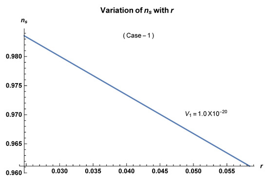
Figure 17. $f(\varphi )=e^{-\frac{\varphi }{2}}$.

The scalar field executes oscillatory behaviour here too, as we demonstrate below. Here $V_E=V_1+V_0{e}^{\varphi }$, and so in view of Equation (19), one can calculate,

$$\begin{array}{c}\frac{3H^2}{V_1}=\frac{{\dot{\sigma }}^2}{2V_1}+\left(1+\frac{V_0}{V_1}{e}^{\varphi }\right)\hfill \end{array}$$

(56)

Again as H falls below $V_1$, and $H\ll V_1$, the above equation can be approximated to, ${\dot{\sigma }}^2=2i^2(V_1+V_0{e}^{\varphi })$, which yields $\dot{\varphi }=i\frac{e^{-\frac{\varphi }{2}}}{{\omega }_0}\sqrt{2(V_1+V_0{e}^{\varphi })}$, where,$\dot{\sigma }={\omega }_0\dot{\varphi }{e}^{\frac{\varphi }{2}}$. Finally, therefore

$$\varphi =ln\left[\frac{1}{4V_0^2}\left(e^{i\frac{\sqrt{2V_0}}{{\omega }_0}t}-2V_0{V}_1+V_0^2{V}_1^2{e}^{-i\frac{\sqrt{2V_0}}{{\omega }_0}t}\right)\right].$$

(57)

The oscillatory behaviour of the scalar field here again assures graceful exit from inflationary regime. In view of (55), $\sigma =2{\omega }_0{e}^{\frac{\varphi }{2}}$, for $\lambda =-1$, which we have considered, hence $\sigma$ also executes oscillatory behaviour.

4. Concluding Remarks

Scalar-tensor theories of gravity are generalizations of the Brans–Dicke theory, in which the coupling parameter is a function of the scalar field, i.e., ${\omega }_{BD}=\omega (\varphi )$, and therefore is a variable. The requirement for such generalization of Brans–Dicke theory generated from the tight constraints on ${\omega }_{BD}$ established by the solar system experiments [58]. There exists various classification of scalar-tensor theory of gravity [59]. In the present manuscript we have considered standard non-minimal coupling, where the coupling parameter $f(\varphi )$ is arbitrary. It has been noticed earlier that such a theory has an in-built symmetry being associated with a conserved current for trace-free fields, such as vacuum and radiation dominated eras for barotropic fluids. In view of such a symmetry, it is possible to fix all the variables of the theory, including the potential function, fixing the form of one of those. In this manuscript, we have chosen different forms of the coupling parameter $f(\varphi )$, which fixed $\omega (\varphi )$ and $V(\varphi )$, to study the cosmological evolution of the very early universe in the context of inflation. Inflation is a quantum mechanical phenomenon, and has occurred around Planck’s era. However, it has been argued that since the radiative corrections to the potential are negligible, hence the inflationary parameters can be computed using the classical Lagrangian [60]. This argument leads in general, to calculate inflationary parameters in view of the classical Lagrangian, which we have done in the present manuscript. The so called unification programmes, which essentially claim to unify early inflationary regime with late-time cosmic acceleration have no credentials, since none of the models passes through a well behaved radiation and early matter dominated era. However, a history of cosmic evolution starting from inflationary regime, followed by a Friedmann-like radiation ($a\propto \sqrt{t}$) and early matter dominated eras ($a\propto t^{\frac{2}{3}}$), that finally ends up to a late-time accelerated universe ($z=0.75$), has already been explored in view of the present model [37]. In this connection, the present model makes a reasonably viable attempt to unify early inflation with late-time cosmic acceleration. Nevertheless earlier, only a single form of the coupling parameter $f(\varphi )$ together with a particular form of $V(\varphi )$ had been treated. Here, we have extended our work considering combinations of a host of power potentials ($V(\varphi )=V_0+V_1{\varphi }^2,V_0+V_1{\varphi }^3,V_0+V_1{\varphi }^4,V_0\varphi +V_1{\varphi }^3,V_0{\varphi }^2+V_1{\varphi }^3,V_0{\varphi }^2+V_1{\varphi }^4,V_0{\varphi }^2+V_1{\varphi }^4-2\sqrt{V_0{V}_1}{\varphi }^3$), together with an exponential potential ($V(\varphi )=V_0+V_1{e}^{\lambda \varphi }$). We find that all the quadratic, cubic, quartic and exponential potentials pass the tighter constraints on inflationary parameters released by latest Planck’s data [40,41] quite comfortably. Further, all these potentials admit graceful exit from inflation, except one case of cubic potential associated with a square potential, i.e., ($V(\varphi )=V_0{\varphi }^2+V_1{\varphi }^3$), for which unfortunately the scalar field does not show up oscillatory behaviour at the end of inflation.

For the purpose of the present analysis, we have translated the non-minimally coupled Jordan’s frame action to the Einstein frame, under conformal transformation. It is therefore worth to make certain comments in this regard. There is an age old debate regarding physical equivalence between the two: Jordan’s and Einstein’s frames, which are related under conformal transformation. Now, indeed if the two formulations are not equivalent, the problem arises in selecting the physically preferred frame. It emerges from the work of several authors, in different contexts on Kaluza–Klein and Brans–Dicke theories, that the formulations of a scalar-tensor theory in the two conformal frames are physically inequivalent [61,62,63,64,65,66,67,68]. Furthermore, the Jordan frame formulation of a scalar-tensor theory is not viable because the energy density of the gravitational scalar field present in the theory is not bounded from below, which amounts to the violation of the weak energy condition [69]). The system therefore is unstable and decays toward a lower and lower energy state ad infinitum [66,67,68]. Although, a quantum system may have states with negative energy density [69,70,71], such feature is not acceptable for a viable classical theory of gravity. In fact, a classical theory must have a ground state that is stable against small perturbations. The violation of the weak energy condition by scalar-tensor theories formulated in the Jordan conformal frame makes them unviable descriptions of classical gravity, while the Einstein frame formulation of scalar-tensor theories is free from such problem. However, in the Einstein frame also there is a violation of the equivalence principle due to the anomalous coupling of the scalar field to ordinary matter. Nevertheless, this violation is small and compatible with the available tests of the equivalence principle [72]. Further, Einstein’s frame is indeed regarded as an important low energy manifestation of compactified theories [72,73,74,75,76,77]. However, in search of Noether symmetries of $F(R)$ theory of gravity, the two frames have been found to be physically equivalent [78]. So although the debate persists, but somehow it is quite relevant to consider Einstein’s frame to be the physical frame. Therefore, in view of the above discussions, it is justified to study the physics associated with non-minimally coupled scalar-tensor theory of gravity, after translating it to the Einstein frame, as we have done in the present article.

References

- Partridge, R.B. 3K: The Cosmic Microwave Background Radiation; Cambridge Univ. Press: Cambridge, UK, 1995. [Google Scholar]
- Turner, M.S.; Kolb, E.W. The Early Universe; Addison-Wesley Publishing Company: Boston, MA, USA, 1990. [Google Scholar]
- Peebles, P.J.E. The Large Scale Structure of the Universe; Princeton Univ. Press: Princeton, NJ, USA, 1980. [Google Scholar]
- Peebles, P.J.E. Principles of Physical Cosmology; Princeton Univ. Press: Princeton, NJ, USA, 1993. [Google Scholar]
- Baumann, D. The Physics of Inflation—A Course for Graduate Students in Particle Physics and Cosmology. arXiv 2015, arXiv:0907.5424. [Google Scholar]
- Sanyal, A.K. Enlightening the dark universe. Indian J. Theor. Phys. 2014, 62, 211–262. [Google Scholar]
- Stelle, K.S. Renormalization of higher-derivative quantum gravity. Phys. Rev. 1977, 953, D16. [Google Scholar] [CrossRef]
- Sen, A. Recent Developments in Superstring Theory. Nucl. Phys. Proc. Suppl. 2001, 94, 35. [Google Scholar] [CrossRef]
- Mukhi, S. String theory: A perspective over the last 25 years. Class. Quant. Grav. 2011, 28, 153001. [Google Scholar] [CrossRef]
- Lahanas, A.B.; Nanopoulos, D.V. The road to no-scale supergravity. Phys. Rep. 1987, 145, 1. [Google Scholar] [CrossRef]
- Ferrara1, S.; Sagnotti, A. Supergravity at 40: Reflections and Perspectives. J. Phys. Conf. Ser. 2016, 873. [Google Scholar] [CrossRef]
- Kenath, A.; Gudennavar, S.B.; Sivaram, C. Dark matter, dark energy, and alternate models: A review. Adv. Space Res. 2017, 60, 166. [Google Scholar]
- Starobinsky, A.A. A new type of isotropic cosmological models without singularity. Phys. Lett. 1980, 99, B91. [Google Scholar] [CrossRef]
- Guth, A.H. Inflationary universe: A possible solution to the horizon and flatness problems. Phys. Rev. D 1981, 23, 347. [Google Scholar] [CrossRef]
- Olive, K.A. Inflation. Phys. Rept. 1990, 190, 307. [Google Scholar] [CrossRef]
- Lyth, D.H.; Riotto, A. Particle physics models of inflation and the cosmological density perturbation. Phys. Rep. 1999, 314, 1–146. [Google Scholar] [CrossRef]
- Liddle, A.R.; Lyth, D.H. Cosmological Inflation and Large-Scale Structure; Cambridge University Press: Cambridge, UK, 2000. [Google Scholar]
- Baumann, D. TASI lectures on inflation. arXiv 2009, arXiv:0907.5424. [Google Scholar]
- Martin, J.; Ringeval, C.; Vennin, V. Encyclopaedia inflationaris. Phys. Dark Univ. 2014, 5–6, 75–235. [Google Scholar] [CrossRef]
- Martin, J.; Ringeval, C.; Trotta, R.; Vennin, V. The best inflationary models after Planck. JCAP 2014, 1403, 39. [Google Scholar] [CrossRef]
- Martin, J. The observational status of cosmic inflation after Planck. In The Cosmic Microwave Background; Fabris, J., Piattella, O., Rodrigues, D., Velten, H., Zimdahl, W., Eds.; Springer: Cham, Switzerland, 2015. [Google Scholar]
- Linde, A.D. A new inflationary universe scenario: A possible solution of the horizon, flatness, homogeneity, isotropy and primordial monopole problems. Phys. Lett. B 1982, 108, 389. [Google Scholar] [CrossRef]
- Albrecht, A.; Steinhardt, P.J. Cosmology for grand unified theories with radiatively induced symmetry breaking. Phys. Rev. Lett. 1982, 48, 1220. [Google Scholar] [CrossRef]
- Press, W.H. Spontaneous production of the Zel’dovich spectrum of cosmological fluctuations. Phys. Scr. 1980, 21, 702. [Google Scholar] [CrossRef]
- Hawking, S.W. The development of irregularities in a single bubble inflationary universe. Phys. Lett. B 1982, 115, 295. [Google Scholar] [CrossRef]
- Starobinsky, A.A. Dynamics of phase transition in the new inflationary universe scenario and generation of perturbations. Phys. Lett. B 1982, 117, 175. [Google Scholar] [CrossRef]
- Guth, A.H.; Pi, S.Y. Fluctuations in the new inflationary universe. Phys. Rev. Lett. 1982, 49, 1110. [Google Scholar] [CrossRef]
- Bardeen, J.M.; Steinhardt, P.J.; Turner, M.S. Spontaneous creation of almost scale-free density perturbations in an inflationary universe. Phys. Rev. D 1983, 28, 679. [Google Scholar] [CrossRef]
- Mukhanov, V.F.; Chibisov, G.V. Quantum fluctuations and a nonsingular universe. JETP Lett. 1981, 33, 532. [Google Scholar]
- Whitt, B. Fourth-order gravity as general relativity plus matter. Phys. Lett. B 1984, 145, 176. [Google Scholar] [CrossRef]
- Wands, D. Extended gravity theories and the Einstein–Hilbert action, Class. Quant. Grav. 1994, 11, 269. [Google Scholar] [CrossRef]
- Horndeski, G.W. Second-order Scalar-tensor field equations in a four-dimentional Space. Int. J. Theor. Phys. 1974, 10, 363. [Google Scholar] [CrossRef]
- Sanyal, A.K. Scalar–tensor theory of gravity carrying a conserved current. Phys. Lett. B 2005, 624, 81. [Google Scholar] [CrossRef][Green Version]
- Sanyal, A.K. Study of symmetry in F(R) theory of gravity. Mod. Phys. Lett. A 2010, 25, 2667. [Google Scholar] [CrossRef]
- Sk, N.; Sanyal, A.K. Field independent cosmic evolution. J. Astrophys. 2013, 2013, 590171. [Google Scholar] [CrossRef]
- Sarkar, K.; Sk, N.; Debnath, S.; Sanyal, A.K. Viability of Noether symmetry of F(R) theory of gravity. Int. J. Theor. Phys. 2013, 52, 1194. [Google Scholar] [CrossRef]
- Tajahmad, B.; Sanyal, A.K. Unified cosmology with scalar–tensor theory of gravity. Eur. Phys. J. 2017, 77, 217. [Google Scholar] [CrossRef]
- Ade, P.A.; Aghanim, N.; Armitage-Caplan, C.; Arnaud, M.; Ashdown, M.; Atrio-Barandela, F.; Aumont, J.; Baccigalupi, C.; Banday, A.J.; Barreiro, R.B.; et al. Planck 2013 results. XVI. Cosmological parameters. Astron. Astrophys. 2014, 571, A16. [Google Scholar]
- Ade, P.A.; Aghanim, N.; Arnaud, M.; Ashdown, M.; Aumont, J.; Baccigalupi, C.; Banday, A.J.; Barreiro, R.B.; Bartlett, J.G.; Bartolo, N.; et al. Planck 2015 resultss. XII. Cosmological parameters. Astron. Astrophys. 2016, 594, A13. [Google Scholar]
- Aghanim, N.; Akrami, Y.; Ashdown, M.; Aumont, J.; Baccigalupi, C.; Ballardini, M.; Banday, A.J.; Barreiro, R.B.; Bartolo, N.; Basak, S.; et al. Planck 2018 Results. VI. Cosmological Parameters, (Planck Collaboration). arXiv 2018, arXiv:1807.06209. [Google Scholar]
- Akrami, Y.; Arroja, F.; Ashdown, M.; Aumont, J.; Baccigalupi, C.; Ballardini, M.; Banday, A.J.; Barreiro, R.B.; Bartolo, N.; Basak, S.; et al. Planck 2018 results. X. Constraints on inflation, (Planck Collaboration). arXiv 2018, arXiv:1807.06211. [Google Scholar]
- Kobayashi, T.; Yamaguchi, M.; Yokoyama, J. Generalised G-inflation: Inflation with most general second order field equation. Prog. Theor. Phys. 2011, 126, 511. [Google Scholar] [CrossRef]
- Kamada, K.; Kobayashi, T.; Yamaguchi, M.; Yokoyama, J. Higgs G-inflation. Phys. Rev. D 2011, 83, 083515. [Google Scholar] [CrossRef]
- Myrzakulov, R.; Sebastiani, L. Scalar tensor Horndeski Models: Simple cosmological applications. Astrophys. Space Sci. 2016, 361, 62. [Google Scholar] [CrossRef]
- Myrzakulov, R.; Sebastiani, L. K-Essence Non-Minimally Coupled with Gauss-Bonnet Invariant for Inflation. Symmetry 2016, 8, 57. [Google Scholar] [CrossRef]
- Gleyzes, J.; Langlois, D.; Piazza, F.; Vernizzi, F. Healthy theories beyond Horndeski. Phys. Rev. Lett. 2015, 114, 211101. [Google Scholar] [CrossRef]
- Gleyzes, J.; Langlois, D.; Piazza, F.; Vernizzi, F. Exploring gravitational theories beyond Horndeski. JCAP 2015, 2, 018. [Google Scholar] [CrossRef]
- Gao, X. Unifying framework for Scalar-tensor theories of gravity. Phys. Rev. D 2014, 90, 081501. [Google Scholar] [CrossRef]
- Zumalaca´rregui, M.; Garci´a-Bellido, J. Trasforming gravity: From derivative couplings to matter to second-order scalar-tensor theories beyond the Horndeski Lagrangian. Phys. Rev. D 2014, 89, 064046. [Google Scholar] [CrossRef]
- Crisostomi, M.; Hull, M.; Koyama, K.; Tasinato, G. Horndeski: Beyond, or not beyond? JCAP 2016, 3, 38. [Google Scholar] [CrossRef]
- Simone, A.D.; Hertzberg, M.P.; Wilczek, F. Running inflation in the standard model. Phys. Lett. B 2009, 678, 1. [Google Scholar] [CrossRef]
- Bhattcharyya, S.; Das, K.; Dutta, K. Attractor models in Scalar-Tensor Theories of Inflation. Int. J. Mod. Phys. 2018, 27, 1850079. [Google Scholar] [CrossRef]
- Park, S.C. Inflation in the nonminimal theory with ‘K(phi)R’ term. AIP Conf. Proc. 2009, 1078, 524. [Google Scholar]
- Park, S.C.; Yamaguchi, S. Inflation by non-minimal coupling. arXiv 2008, arXiv:0801.1722. [Google Scholar] [CrossRef]
- Kleinert, H.; Mustapic, I. Decay rates of metastable states in cubic potential by variational perturbation theory. Int. J. Mod. Phys. A 1996, 11, 4383. [Google Scholar] [CrossRef]
- Falconi, M.; Lacomba, E.A.; Vidal, C. The flow of classical mechanical cubic potential systems. Discont. Cont. Dyn. Syst. 2004, 11, 827. [Google Scholar] [CrossRef]
- Wartak, M.S.; Krzeminski, S. On tunnelling in the cubic potential. J. Phys. A: Math. Gen. 1989, 22, L1005. [Google Scholar] [CrossRef]
- Will, C.M. The confrontation between general relativity and experiment. Living Rev. Rel. 2014, 17, 4. [Google Scholar] [CrossRef] [PubMed]
- Quiros, I.; De Arcia, R.; García-Salcedo, R.; Gonzalez, T.; Horta-Rangel, F.A. An issue with the classification of the scalar-tensor theories of gravity. Int. J. Mod. Phys. D 2020, 29, 7. [Google Scholar] [CrossRef]
- Bezrukov, F.L.; Shaposhnikov, M. The standard model Higgs boson as the inflaton. Phys. Lett. B 2008, 659, 703. [Google Scholar] [CrossRef]
- Bombelli, L.; Koul, R.K.; Kunstatter, G.; Lee, J.; Sorkin, R.D. On energy in 5-dimensional gravity and the mass of the Kaluza-Klein monopole. Nucl. Phys. B 1987, 289, 735. [Google Scholar] [CrossRef]
- Sokolowski, L.M.; Golda, Z.A. Instability of Kaluza-Klein cosmology. Phys. Lett. B 1987, 195, 349. [Google Scholar] [CrossRef]
- Sokolowski, L.M. Uniqueness of the metric line element in dimensionally reduced theories. Class. Quant. Grav. 1989, 6, 59. [Google Scholar] [CrossRef]
- Cho, Y.M. Unified cosmology. Phys. Rev. D 1990, 41, 2462. [Google Scholar] [CrossRef]
- Cho, Y.M. Violation of equivalence principle in Brans–Dicke theory. Class. Quant. Grav. 1997, 14, 2963. [Google Scholar] [CrossRef]
- Magnano, G.; Sokolowski, L.M. On Physical Equivalence between Nonlinear Gravity Theories. Phys. Rev. D 1994, 50, 5039. [Google Scholar] [CrossRef]
- Faraoni, V.; Gunzig, E.; Nardone, P. Conformal transformations in classical gravitational theories and in cosmology. Fund. Cosmic Phys. 1998, 20, 121. [Google Scholar]
- Faraoni, V.; Gunzig, E.; Nardone, P. Einstein Frame or Jordan Frame? Int. J. Theory Phys. 1999, 38, 217. [Google Scholar] [CrossRef]
- Witten, E. Instability of the Kaluza-Klein vacuum. Nucl. Phys. B 1982, 195, 481. [Google Scholar] [CrossRef]
- Ford, L.H.; Roman, T.A. Cosmic flashing in four dimensions. Phys. Rev. D 1992, 46, 1328. [Google Scholar] [CrossRef] [PubMed]
- Ford, L.H.; Roman, T.A. Averaged energy conditions and quantum inequalities. Phys. Rev. D 1995, 51, 4277. [Google Scholar] [CrossRef]
- Cho, Y.M. Reinterpretation of Jordan-Brans–Dicke theory and Kaluza-Klein cosmology. Phys. Rev. Lett. 1992, 68, 3133. [Google Scholar] [CrossRef] [PubMed]
- Taylor, T.R.; Veneziano, G. Dilaton couplings at large distances. Phys. Lett. B 1988, 213, 450. [Google Scholar] [CrossRef]
- Cvetic, M. Low energy signals from moduli. Phys. Lett. B 1989, 229, 41. [Google Scholar] [CrossRef]
- Ellis, J.; Kalara, S.; Olive, K.A.; Wetterich, C. Density-dependent couplings and astrophysical bounds on light scalar particles. Phys. Lett. B 1989, 228, 264. [Google Scholar] [CrossRef]
- Damour, T.; Polyakov, A.M. The String Dilaton and a Least Coupling Principle. Nucl. Phys. B 1994, 423, 532. [Google Scholar] [CrossRef]
- Damour, T.; Polyakov, A.M. String theory and gravity. Gen. Rel. Gravit. 1994, 26, 1171. [Google Scholar] [CrossRef]
- Sk, N.; Sanyal, A.K. On the equivalence between different canonical forms of F(R) theory of gravity. Int. J. Mod. Phys. D 2018, 27, 1850085. [Google Scholar] [CrossRef]
© 2020 by the authors. Licensee MDPI, Basel, Switzerland. This article is an open access article distributed under the terms and conditions of the Creative Commons Attribution (CC BY) license (http://creativecommons.org/licenses/by/4.0/).