On Two-Derivative Runge–Kutta Type Methods for Solving u‴ = f(x,u(x)) with Application to Thin Film Flow Problem

Abstract

A class of explicit Runge–Kutta type methods with the involvement of fourth derivative, denoted as two-derivative Runge–Kutta type (TDRKT) methods, are proposed and investigated for solving a special class of third-order ordinary differential equations in the form $u^{‴}\left(x\right)=f(x,u\left(x\right))$. In this paper, two stages with algebraic order four and three stages with algebraic order five are presented. The derivation of TDRKT methods involves single third derivative and multiple evaluations of fourth derivative for every step. Stability property of the methods are analysed. Accuracy and efficiency of the new methods are exhibited through numerical experiments.

1. Introduction

In this study, we consider the special class of third-order ordinary differential equations (ODEs) in the form:

$$\begin{array}{c}\hfill \left\{\begin{array}{c}{u}^{‴}\left(x\right)=f(x,u\left(x\right)),\hfill \\ u\left(x_0\right)=u_0,u^{\prime }\left(x_0\right)=u_0^{\prime },u^{″}\left(x_0\right)=u_0^{″}x\in [x_0,x_{end}],\hfill \end{array}\right.\end{array}$$

(1)

where $u\in {\Re }^N,f:=\Re \times {\Re }^N\to {\Re }^N$ is a continuous vector function.

Third-order ordinary differential equations are principally used to outlook and estimate the pattern of scientific problems, including thin film flow, electrical circuits, momentum transport of viscoelastic fluids in porous channels, and other disciplines. A popular approach for solving third-order ODEs is to convert third-order ODEs into a system of first-order ODEs and solve it with traditional first-order methods such as Runge–Kutta method, linear multistep method, and predictor–corrector method. The disadvantage of using this particular way is that it generates higher local truncation error and rounding error that leads to inaccuracy of numerical approximations. This issue led to the construction of direct methods in solving third-order ODEs to improve the accuracy of methods.

Some efforts have been done by several researchers on deriving direct solving methods. Omar et al. [1] proposed a block hybrid method for higher-order initial value problems in the form of a rapidly convergent series. Agboola et al. [2] derived differential transformation method (DTM) with Taylor series-based for solving third-order ODEs. Khataybeh et al. [3] introduced operational matrices of Bernstein polynomials method for solving a class of third-order ODEs directly. Tang and Zhang [4] constructed continuous-stage Runge–Kutta–Nyström methods with Legendre expansion technique in conjunction with the symmetric conditions for solving second-order ordinary differential equations. On the other hand, certain two derivative Runge–Kutta–Nyström methods with inclusion of third derivative have been presented to solve second order ODEs (see Fang et al. [5], Chen et al. [6], Ehigie et al. [7], and Mohamed et al. [8]).

In this research paper, traditional two-derivative direct Runge–Kutta scheme is modified by removing increment function ${\displaystyle \sum _{i=1}^s}{b}_i{k}_i$ in third derivative and replaced it with single function $f(x,u(x\left)\right)$ from the third-order numerical problem as well as inserting evaluation function with fourth derivative in the formulation.

The objective of this paper is to design high-order two-derivative Runge–Kutta type (TDRKT) methods with minimal number of functional evaluation, consisting of two-stages fourth-order and three-stages fifth-order. In Section 2, general formulation of TDRKT methods is proposed. In Section 3, construction of TDRKT method based on rooted tree will be shown and the methods with two-stages fourth-order and three-stages fifth-order are derived. The linear stability analysis of TDRKT methods is discussed. In Section 4, capability of TDRKT methods is illustrated through the numerical test. Numerical results of TDRKT methods and other existing methods are exhibited in Section 5. This paper ends in Section 6 with the discussion and conclusion.

2. The Formulation of TDRKT Methods

TDRKT methods are derived with the inclusion of fourth derivative, $u^{\left(iv\right)}\left(x\right)$, in the formulation as shown below:

$$\begin{array}{cc}\hfill u^{\left(iv\right)}\left(x\right)=g(x,u,u^{{}^{\prime }})=& f_x(x,u,u^{{}^{\prime }})+f_u(x,u,u^{{}^{\prime }})u^{{}^{\prime }}.\hfill \end{array}$$

(2)

s-stage TDRKT methods consist of multiple evaluations in fourth derivative and single evaluation in third derivative that are expressed as follows:

$$\begin{array}{cc}{u}_{n+1}=\hfill & u_n+h{u}_n^{{}^{\prime }}+\frac{h^2}{2}{u}_n^{{}^{″}}+\frac{h^3}{6}f(x_n,u_n)+h^4\sum _{i=1}^s{b}_{i}g\left(x_n+c_{i}h,U_i,U_i^{{}^{\prime }}\right),\hfill \\ u_{n+1}^{{}^{\prime }}=\hfill & u_n^{{}^{\prime }}+h{u}_n^{{}^{″}}+\frac{h^2}{2}f(x_n,u_n)+h^3\sum _{i=1}^s{b}_i^{{}^{\prime }}g\left(x_n+c_{i}h,U_i,U_i^{{}^{\prime }}\right),\hfill \\ u_{n+1}^{{}^{″}}=\hfill & u_n^{{}^{″}}+hf(x_n,u_n)+h^2\sum _{i=1}^s{b}_i^{{}^{″}}g\left(x_n+c_{i}h,U_i,U_i^{{}^{\prime }}\right),\hfill \end{array}$$

where

$$\begin{array}{cc}\hfill U_i=& u_n+c_{i}h{u}_n^{{}^{\prime }}+\frac{{\left(c_{i}h\right)}^2}{2}{u}_n^{{}^{″}}+\frac{{\left(c_{i}h\right)}^3}{6}f(x_n,u_n)+h^4\sum _{j=1}^s{a}_{i,j}g\left(x_n+c_{i}h,U_j,U_j^{{}^{\prime }}\right),\hfill \\ \hfill U_i^{{}^{\prime }}=& u_n^{{}^{\prime }}+c_{i}h{u}_n^{{}^{″}}+\frac{{\left(c_{i}h\right)}^2}{2}f(x_n,u_n)+h^3\sum _{j=1}^s{\widehat{a}}_{i,j}g\left(x_n+c_{i}h,U_j,U_j^{{}^{\prime }}\right),\hfill \end{array}$$

(3)

where $c_i,b_i,b_i^{\prime },b_i^{″},{\overline{a}}_{i,j}{\widehat{a}}_{i,j},i,j=1,2,...,s\in \mathbb{Z}$. In addition, Equation (3) can be expressed in Butcher’s tableau (see Table 1):

Table 1. Two-derivative Runge–Kutta type (TDRKT) methods in Butcher tableau.

C	a	$\widehat{\mathit{a}}$
	$b^T$	$b^{{}^{\prime }T}$	$b^{{}^{″}T}$

TDRKT methods are implicit methods if $a_{i,j}$ and ${\widehat{a}}_{i,j}$ are not equal to 0 for $i\le j$, and are explicit methods otherwise. Unlike the traditional two-derivative Runge–Kutta type method, TDRKT methods simply comprise of one function evaluation of f and multiple function evaluations of g per step, and thus, having lower amount of total function evaluations than the existing two-derivative Runge–Kutta type methods which consist of numerous evaluations of f and g per step depending on the amount of stages.

3. Construction of TDRKT Methods

In this section, all coefficients of TDRKT methods, $c_i,b_i,b_i^{\prime },b_i^{″},a_{i,j}{\widehat{a}}_{i,j}$ will be determined. For obtaining a general formula for higher derivatives of analytical solution of problem (3), we consider the expression of first to seventh derivatives of the analytical solution $u\left(x\right)$ at $x=x_0$.

$$\begin{array}{ccc}{u}^{\left(1\right)}\hfill & =\hfill & u^{\prime },u^{\left(2\right)}=u^{″},u^{\left(3\right)}=f,u^{\left(4\right)}=g,u^{\left(5\right)}=g_u^{\prime }{u}^{\prime }+g_{u^{\prime }}^{\prime }{u}^{″},\hfill \\ u^{\left(6\right)}\hfill & =\hfill & g_{uu}^{\left(2\right)}{u}^{\prime 2}+2g_{u{u}^{\prime }}^{\left(2\right)}{u}^{\prime }{u}^{″}+g_{u^{\prime }{u}^{\prime }}^{\left(2\right)}{u}^{″2}+g_u^{\prime }{u}^{″}+g_{u^{\prime }}^{\prime }f,\hfill \\ u^{\left(7\right)}\hfill & =\hfill & g_{uuu}^{\left(3\right)}{u}^{\prime 3}+3g_{uu{u}^{\prime }}^{\left(3\right)}{u}^{\prime 2}{u}^{″}+3g_{u{u}^{\prime }{u}^{\prime }}^{\left(3\right)}{u}^{\prime }{u}^{″2}+g_{u^{\prime }{u}^{\prime }{u}^{\prime }}^{\left(3\right)}{u}^{″3}+3g_{uu}^{\left(2\right)}{u}^{\prime }{u}^{″}\hfill \\ \hfill & +\hfill & 3g_{u{u}^{\prime }}^{\left(2\right)}{u}^{\prime }{f}^{\prime }+3g_{u^{\prime }{u}^{\prime }}^{\left(2\right)}{u}^{″}f+g_{u}f+g_{u^{\prime }}g+3g_{u{u}^{\prime }}{u}^{″2}.\hfill \end{array}$$

(4)

Fundamental of the set of rooted trees for TDRKT methods are described and analysed as follows (see Chen et al. [6]):

Definition 1.

The set $RT$ of rooted trees is recursively interpreted as

(i)

The graphexpressed as ${\tau }_1$, with one meagre vertex (root of the rooted tree); the graphexpessed as ${\tau }_2$; the graphdenoted as ${\tau }_3$; and lastly,denoted as ${\tau }_4$;

(ii)

If $t_1,\dots ,t_r,t_{r+1},\dots ,t_m,t_{m+1},\dots ,t_n,t_{n+1},\dots ,t_s\in RT,t_{n+1},\dots ,t_s$ are different from ${\tau }_1$, then the graph can be obtained as the roots of $t_1,\dots ,t_r$ connecting downward to white circle vertex, combining the roots of $t_{r+1},\dots ,t_m$ into this black triangle vertex, followed by joining the roots $t_{m+1},\dots ,t_n$ downward to white rectangle vertex and subsequently to the roots $t_n,t_{n+1},\dots ,t_s$ into a new black circle vertex (root of $RT$). It is expressed as

$$\begin{array}{c}\hfill \begin{array}{c}\hfill t={\left[t_1,\dots ,t_r,<t_{r+1},\dots ,t_m>,<t_{m+1},\dots ,t_n>,<t_{n+1},\dots ,t_s>\right]}_4,\end{array}\end{array}$$

(5)

in whichis root of the rooted tree t.

The criteria of producing the following rooted tree are as follows:

(i)

The meagre vertex is the root of every rooted tree.

(ii)

The offspring of meagre vertex must consist of only one white circle vertex.

(ii)

The offspring of white circle vertex must consist of only one black triangle vertex.

(iv)

The offspring of black triangle vertex must consist of only one white rectangle vertex.

Definition 2.

Order of integer function $\rho :RT\to \mathbb{N}$ is expressed as follows:

(i)

$\rho \left({\tau }_1\right)=1,\rho \left({\tau }_2\right)=2,\rho \left({\tau }_3\right)=3,\rho \left({\tau }_4\right)=4,$

(ii)

for $t={\left[t_1,\dots ,t_r,<t_{r+1},\dots ,t_m>,<t_{m+1},\dots ,t_n>\right]}_3\in RT$,

$$\begin{array}{c}\hfill \rho \left(t\right)=4+\sum _{i=1}^r\rho \left(t_i\right)+\sum _{i=r+1}^m(\rho \left(t_i\right)-1)+\sum _{i=m+1}^n(\rho \left(t_i\right)-2).\end{array}$$

For every $t\in RT$, the order ρ represents the amount of vertices t. The set comprised of all rooted trees with order k is expressed as $R{T}_k$.

Definition 3.

For every tree $t\in RT$, the fundamental differential is a vector function $F\left(t\right):{\mathbb{R}}^d\times {\mathbb{R}}^d\times {\mathbb{R}}^d\to {\mathbb{R}}^d$ expressed as follows:

(i)

$\begin{array}{c}F\left({\tau }_1\right)(u,u^{\prime },u^{″})=u^{\prime },F\left({\tau }_2\right)(u,u^{\prime },u^{″})=u^{″},F\left({\tau }_3\right)(u,u^{\prime },u^{″})=f\left(u\right),\hfill \\ F\left({\tau }_4\right)(u,u^{\prime },u^{″})=f^{\prime }\left(u\right)=g(u,u^{\prime })\hfill \end{array}$;

(ii)

for $t={\left[t_1,\dots ,t_r,<t_{r+1},\dots ,t_m>,<t_{m+1},\dots ,t_n>,<t_{n+1},\dots ,t_s>\right]}_4\in RT$,

$$\begin{array}{c}\hfill \begin{array}{c}\hfill F\left(t\right)(u,u^{\prime },u^{″})=\frac{{\partial }^{n}g}{\partial u^r\partial u^{\prime m-r}\partial u^{″n-m}}\left(u,u^{\prime },u^{″}\right)\left[F\left(t_1\right)(u,u^{\prime },u^{″}),...,F\left(t_n\right)(u,u^{\prime },u^{″})\right].\end{array}\end{array}$$

(6)

Definition 4.

An integer function $\sigma :RT\to \mathbb{N}$ is recursively described as follows:

(i)

$\sigma \left({\tau }_1\right)=\sigma \left({\tau }_2\right)=\sigma \left({\tau }_3\right)=\sigma \left({\tau }_4\right)=1$;

(ii)

for $t=\left[t_1^{{\mu }_1},\dots ,t_r^{{\mu }_r},<t_{r+1}^{{\mu }_{r+1}},\dots ,t_m^{{\mu }_m}>,<t_{m+1}^{{\mu }_{m+1}},\dots ,t_n^{{\mu }_n}>\right]\in RT,$ with $t_1,\dots ,t_r$, $t_{r+1},\dots ,t_m$ and $t_{m+1},\dots ,t_n$ distinct,

$$\begin{array}{c}\hfill \sigma \left(t\right)=\prod _{i=1}^n{\mu }_i!\left(\sigma {\left(t_i\right)}^{{\mu }_i}\right),\end{array}$$

in which ${\mu }_i$ is the product of $t_i$ for $i=1,\dots ,n$.

Theorem 1.

Given the analytical solution $u(x_0+h)$ of Equation (1) is B-series $B(e,u_0,u_0^{\prime },u_0^{″})$ with real function e prescribed on $RT\cup \left\{\varnothing \right\}$, then

$$\begin{array}{c}\hfill e\left(\varnothing \right)=1,e\left({\tau }_1\right)=1,e\left({\tau }_2\right)=\frac{1}{2},e\left({\tau }_3\right)=\frac{1}{6},\end{array}$$

and for $t={\left[t_1,\dots ,t_r,<t_{r+1},\dots ,t_m>,<t_{m+1},\dots ,t_n>\right]}_3$,

$$\begin{array}{c}\hfill e\left(t\right)=\frac{1}{\rho \left(t\right)\left(\rho \right(t)-1)\left(\rho \right(t)-2)}\prod _{i=1}^{r}e\left(t_i\right)\prod _{i=r+1}^m\rho \left(t_i\right)e\left(t_i\right)\prod _{i=m+1}^n\rho \left(t_i\right)(\rho \left(t_i\right)-1)e\left(t_i\right).\end{array}$$

Proof. 

By assumption,

$$\begin{array}{c}\hfill \begin{array}{ccc}u(x_0+h)\hfill & =\hfill & B(e,u_0,u_0^{\prime },u_0^{″})\hfill \\ \hfill & =\hfill & e\left(\varnothing \right)u_0+he\left({\tau }_1\right)u^{\prime }\left(0\right)+h^{2}e\left({\tau }_2\right)u_0^{″}+h^{3}e\left({\tau }_3\right)f\left(u_0\right)+\sum _{t\in RT\setminus \{{\tau }_1,{\tau }_2,{\tau }_3\}}\frac{h^{\rho \left(t\right)}}{\sigma \left(t\right)}e\left(t\right)F\left(t\right)(u_0,u_0^{\prime },u_0^{″}).\hfill \end{array}\end{array}$$

(7)

The first two derivatives of $y(x_0+h)$ are shown below:

$$\begin{array}{c}\begin{array}{ccc}{\left(u(x_0+h)\right)}^{\prime }\hfill & =\hfill & e\left({\tau }_1\right)u^{\prime }\left(0\right)+2he\left({\tau }_2\right)u_0^{″}+3h^{2}e\left({\tau }_3\right)f\left(u_0\right)+\sum _{t\in RT\setminus \{{\tau }_1,{\tau }_2,{\tau }_3\}}\frac{\rho \left(t\right)h^{\rho \left(t\right)-1}}{\sigma \left(t\right)}e\left(t\right)F\left(t\right)(u_0,u_0^{\prime },u_0^{″})\hfill \\ \hfill & =\hfill & B\left(\frac{\rho }{h}e,u_0,u_0^{\prime },u_0^{″}\right),\hfill \\ {\left(u(x_0+h)\right)}^{″}\hfill & =\hfill & 2e\left({\tau }_2\right)u_0^{″}+6he\left({\tau }_3\right)f\left(u_0\right)+\sum _{t\in RT\setminus \{{\tau }_1,{\tau }_2,{\tau }_3\}}\frac{\rho \left(t\right)(\rho \left(t\right)-1)h^{\rho \left(t\right)-2}}{\sigma \left(t\right)}e\left(t\right)F\left(t\right)(u_0,u_0^{\prime },u_0^{″})\hfill \\ \hfill & \hfill =& B\left(\frac{\rho (\rho -1)}{h^2}e,u_0,u_0^{\prime },u_0^{″}\right).\hfill \end{array}\hfill \end{array}$$

(8)

Besides,

$$\begin{array}{c}\hfill \begin{array}{c}\hfill g\left(B\left(e,u_0,u_0^{\prime },u_0^{″}\right),B\left(\frac{\rho }{h}e,u,u^{\prime },u^{″}\right)\right)=e^{″}\left({\tau }_3\right)f\left(u_0\right)+\sum _{t\in RT\setminus \{{\tau }_1,{\tau }_2,{\tau }_3\}}\frac{h^{\rho \left(t\right)-2}}{\sigma \left(t\right)}{e}^{″}\left(t\right)F\left(t\right)(u_0,u_0^{\prime }),\end{array}\end{array}$$

where $e^{″}\left({\tau }_2\right)=1$ and for $t={\left[t_1,\dots ,t_r,<t_{r+1},\dots ,t_m>,<t_{m+1},\dots ,t_n>\right]}_3\in RT\setminus \{{\tau }_1,{\tau }_2,{\tau }_3\}$,

$$\begin{array}{c}\hfill e^{″}\left(t\right)=\prod _{i=1}^{r}e\left(t_i\right)\prod _{i=r+1}^m\rho \left(t_i\right)e\left(t_i\right)\prod _{i=m+1}^n\rho \left(t_i\right)(\rho \left(t_i\right)-1)e\left(t_i\right).\end{array}$$

(9)

Combining (7) and (8) into autonomous problem of (1) and comparing coefficients of the fundamental differential on both sides yield

$$\begin{array}{c}\hfill e\left({\tau }_2\right)=\frac{1}{2},e\left({\tau }_3\right)=\frac{1}{6},\end{array}$$

and for $t={\left[t_1,\dots ,t_r,<t_{r+1},\dots ,t_m>,<t_{m+1},\dots ,t_n>\right]}_3\in RT\setminus \{{\tau }_1,{\tau }_2,{\tau }_3\}$,

$$\begin{array}{c}\hfill e\left(t\right)=\frac{1}{\rho \left(t\right)\left(\rho \right(t)-1)\left(\rho \right(t)-2)}\prod _{i=1}^{r}e\left(t_i\right)\prod _{i=r+1}^m\rho \left(t_i\right)e\left(t_i\right)\prod _{i=m+1}^n\rho \left(t_i\right)(\rho \left(t_i\right)-1)e\left(t_i\right).\end{array}$$

 □

Through Taylor series expansion of $u(x_0+h)$ around $h=0,e\left(\varnothing \right)=e\left({\tau }_1\right)=1,e\left({\tau }_2\right)=\frac{1}{2},e\left({\tau }_3\right)=\frac{1}{6}.$

For every $t\in RT$, elements of rooted tree, density and positive integer can be defined as $\gamma \left(t\right)=\frac{1}{e\left(t\right)}$ and $\alpha \left(t\right)=\frac{\rho \left(t\right)!}{\sigma \left(t\right)\gamma \left(t\right)}$. Two propositions can be derived based on Theorem 1.

Proposition 1.

For every tree $t\in RT$, density $\gamma \left(t\right)$ is defined as positive integer function on set $RT$ (see Chen et al. [6]).

(i)

$\gamma \left({\tau }_1\right)=1,\gamma \left({\tau }_2\right)=2,\gamma \left({\tau }_3\right)=6$;

(ii)

for $t={\left[t_1,\dots ,t_r,<t_{r+1},\dots ,t_m>,<t_{m+1},\dots ,t_n>\right]}_3\in RT,$$\gamma \left(t\right)=\rho \left(t\right)(\rho \left(t\right)-1)(\rho \left(t\right)-2){\prod }_{i=1}^r\gamma \left(t_i\right){\prod }_{i=r+1}^m\frac{\gamma \left(t_i\right)}{\rho \left(t_i\right)}{\prod }_{i=m+1}^n\frac{\gamma \left(t_i\right)}{\rho \left(t_i\right)(\rho \left(t_i\right)-1)}.$

Proposition 2.

For every tree $t\in RT$, positive integer $\alpha \left(t\right)$ is fulfilled (see Chen et al. [6]).

(i)

$\alpha \left({\tau }_1\right)=1,\alpha \left({\tau }_2\right)=1,\alpha \left({\tau }_3\right)=1$;

(ii)

for $t={\left[t_1^{{\mu }_1},\dots ,t_r^{{\mu }_r},<t_{r+1}^{{\mu }_{r+1}},\dots ,t_m^{{\mu }_m}>,<t_{m+1}^{{\mu }_{m+1}},\dots ,t_n^{{\mu }_n}>\right]}_3\in RT,$ whereby $t_1,\dots ,t_r$ distinct, $t_{r+1},\dots ,t_m$ distinct and $t_{m+1},\dots ,t_n$ distinct,

$$\begin{array}{c}\hfill \alpha \left(t\right)=(\rho \left(t\right)-3)!\prod _{i=1}^r\frac{1}{{\mu }_i!}{\left(\frac{\alpha \left(t_i\right)}{\rho \left(t_i\right)!}\right)}^{{\mu }_i}\prod _{i=r+1}^m\frac{1}{{\mu }_i!}{\left(\frac{\alpha \left(t_i\right)}{(\rho \left(t_i\right)-1)!}\right)}^{{\mu }_i}·\prod _{i=m+1}^n\frac{1}{{\mu }_i!}{\left(\frac{\alpha \left(t_i\right)}{(\rho \left(t_i\right)-2)!}\right)}^{{\mu }_i},\end{array}$$

(10)

where ${\mu }_i$ is the product of $t_i,i=1,\dots ,n.$

Here, B-series of TDRKT methods can be defined as

$$\begin{array}{c}\hfill B(\beta ,u,u^{\prime },u^{″})=\beta \left(\varnothing \right)u+\sum _{t\in RT}\frac{h^{\rho \left(t\right)}}{\rho \left(t\right)!}\beta \left(t\right)\gamma \left(t\right)\alpha \left(t\right)F\left(t\right)(u,u^{\prime },u^{″}),\end{array}$$

(11)

and $g\left(B(\overline{\beta },u,u^{\prime },u^{″}),B(\widehat{\beta },u,u^{\prime },u^{″})\right)$ can be denoted as

$$\begin{array}{c}\hfill \begin{array}{c}\hfill g\left(B(\overline{\beta },u,u^{\prime },u^{″}),B(\widehat{\beta },u,u^{\prime },u^{″})\right)=\sum _{t\in RT\setminus \{{\tau }_1,{\tau }_2,{\tau }_3\}}\frac{h^{\rho \left(t\right)-4}}{\rho \left(t\right)!}{\beta }^{\left(4\right)}\left(t\right)\gamma \left(t\right)\alpha \left(t\right)F\left(t\right)(u,u^{\prime },u^{″}).\end{array}\end{array}$$

(12)

3.1. Analytical Solution and Exact Derivative on B-Series

Theorem 2.

Exact solution $u(x_0+h)$ and the derivative $u^{\prime }(x_0+h)$ and $u^{″}(x_0+h)$ of the problem (1) have the forms as follows:

$$\begin{array}{c}\begin{array}{ccc}u(x_0+h)\hfill & =\hfill & u_0+\sum _{t\in RT}\frac{h^{\rho \left(t\right)}}{\rho \left(t\right)!}\alpha \left(t\right)F\left(t\right)(u_0,u_0^{\prime },u_0^{″})=B\left(\frac{\alpha \sigma }{\rho !},u_0,u_0^{\prime },u_0^{″}\right)=B\left(\frac{1}{\gamma },u_0,u_0^{\prime },u_0^{″}\right),\hfill \\ u^{\prime }(x_0+h)\hfill & =\hfill & u_0^{\prime }+\sum _{t\in RT}\frac{h^{\rho \left(t\right)-1}}{\left(\rho \right(t)-1)!}\alpha \left(t\right)F\left(t\right)(u_0,u_0^{\prime },u_0^{″})=B\left(\frac{\alpha \sigma }{h(\rho -1)!},u_0,u_0^{\prime },u_0^{″}\right)\hfill \\ \hfill & =\hfill & B\left(\frac{\rho }{h\gamma },u_0,u_0^{\prime },u_0^{″}\right),\hfill \\ u^{″}(x_0+h)\hfill & =\hfill & u_0^{″}+\sum _{t\in RT}\frac{h^{\rho \left(t\right)-2}}{\left(\rho \right(t)-2)!}\alpha \left(t\right)F\left(t\right)(u_0,u_0^{\prime },u_0^{″})=B\left(\frac{\alpha \sigma }{h^2(\rho -2)!},u_0,u_0^{\prime },u_0^{″}\right)\hfill \\ \hfill & =\hfill & B\left(\frac{\rho (\rho -1)}{h^2\gamma },u_0,u_0^{\prime },u_0^{″}\right).\hfill \end{array}\hfill \end{array}$$

(13)

Proof. 

The conclusion is based on Theorem 1 and expression (11). □

3.2. Numerical Solution and Numerical Derivative on B-Series

B-series based on TDRKT methods are developed regarding numerical solution of $u_1$ and its numerical derivatives $u_1^{\prime }$ and $u_1^{″}$ of the problem (1) produced by TDRKT methods, $U_i$ and $U_i^{\prime }$ are expanded as B-series as $U_i=B({\overline{\Psi }}_i,u_0,u_0^{\prime },u_0^{″})$ and $U_i^{\prime }=B(\frac{\rho }{h}{\widehat{\Psi }}_i,u_0,u_0^{\prime },u_0^{″})$, respectively. Hence, the first three equations in (3) become

$$\begin{array}{c}\begin{array}{c}B({\overline{\Psi }}_i,u_0,u_0^{\prime },u_0^{″})=u_0+c_{i}h{u}_0^{\prime }+\frac{{\left(c_{i}h\right)}^2}{2}{u}_0^{″}+\frac{{\left(c_{i}h\right)}^3}{6}{f}_0+h^4\sum _{j=1}^s{A}_{i,j}g\left(B({\overline{\Psi }}_j,u_0,u_0^{\prime },u_0^{″}),B\left(\frac{\rho }{h}{\widehat{\Psi }}_j,u_0,u_0^{\prime },u_0^{″}\right)\right),\hfill \\ B\left(\frac{\rho }{h}{\widehat{\Psi }}_i,u_0,u_0^{\prime },u_0^{″}\right)=u_0^{\prime }+c_{i}h{u}_0^{″}+\frac{{\left(c_{i}h\right)}^2}{2}{f}_0+h^3\sum _{j=1}^s{\widehat{A}}_{i,j}g\left(B({\overline{\Psi }}_j,u_0,u_0^{\prime },u_0^{″}),B\left(\frac{\rho }{h}{\widehat{\Psi }}_j,u_0,u_0^{\prime },u_0^{″}\right)\right).\hfill \end{array}\hfill \end{array}$$

(14)

Referring to (11) and (12), the previous three equations can be expressed as

$$\begin{array}{c}{\overline{\Psi }}_i\left(\varnothing \right)u+\sum _{t\in RT}\frac{h^{\rho \left(t\right)}}{\rho \left(t\right)!}{\overline{\Psi }}_i\left(t\right)\gamma \left(t\right)\alpha \left(t\right)F\left(t\right)(u_0,u_0^{\prime },u_0^{″})\hfill \\ =u_0+c_{i}h{u}_0^{\prime }+\frac{{\left(c_{i}h\right)}^2}{2}{u}_0^{″}+\frac{{\left(c_{i}h\right)}^3}{6}{f}_0+\sum _{j=1}^s\sum _{RT\setminus \{{\tau }_1,{\tau }_2,{\tau }_3\}}\frac{h^{\rho \left(t\right)}}{\rho \left(t\right)!}{A}_{i,j}{\Psi }_j^{\left(4\right)}\left(t\right)\gamma \left(t\right)\alpha \left(t\right)F\left(t\right)(u_0,u_0^{\prime },u_0^{″}),\hfill \\ \sum _{t\in RT}\frac{h^{\rho \left(t\right)-1}}{\left(\rho \right(t)-1)!}{\widehat{\Psi }}_i\left(t\right)\gamma \left(t\right)\alpha \left(t\right)F\left(t\right)(u_0,u_0^{\prime },u_0^{″})\hfill \\ =u_0^{\prime }+c_{i}h{u}_0^{″}+\frac{{\left(c_{i}h\right)}^2}{2}{f}_0+\sum _{j=1}^s\sum _{RT\setminus \{{\tau }_1,{\tau }_2,{\tau }_3\}}\frac{h^{\rho \left(t\right)-1}}{\rho \left(t\right)!}{\widehat{A}}_{i,j}{\Psi }_j^{\left(4\right)}\left(t\right)\gamma \left(t\right)\alpha \left(t\right)F\left(t\right)(u_0,u_0^{\prime },u_0^{″}).\hfill \end{array}$$

(15)

It follows

$$\begin{array}{c}\hfill \begin{array}{c}{\overline{\Psi }}_i\left(\varnothing \right)=1,{\overline{\Psi }}_i\left({\tau }_1\right)=c_i,{\overline{\Psi }}_i\left({\tau }_2\right)=\frac{{\left(c_i\right)}^2}{2},{\overline{\Psi }}_i\left({\tau }_3\right)=\frac{{\left(c_i\right)}^3}{6},\hfill \\ {\overline{\Psi }}_i\left({\tau }_4\right)=\sum _{j=1}^s{A}_{i,j}{\Psi }_j^{\left(4\right)}=\sum _{j=1}^s{A}_{i,j},{\widehat{\Psi }}_i\left({\tau }_1\right)=1,{\widehat{\Psi }}_i\left({\tau }_2\right)=c_i,{\widehat{\Psi }}_i\left({\tau }_3\right)=\frac{{\left(c_i\right)}^2}{2},\hfill \\ {\widehat{\Psi }}_i\left({\tau }_4\right)=\sum _{j=1}^s{\widehat{A}}_{i,j}{\Psi }_j^{\left(4\right)}=\sum _{j=1}^s{\widehat{A}}_{i,j},\hfill \end{array}\end{array}$$

(16)

and

$$\begin{array}{c}\hfill \begin{array}{c}\hfill {\overline{\Psi }}_i\left(t\right)=\sum _{j=1}^s{A}_{i,j}{\Psi }_j^{\left(4\right)}\left(t\right),{\widehat{\Psi }}_i\left(t\right)=\sum _{j=1}^s{\widehat{A}}_{i,j}{\Psi }_j^{\left(4\right)}\left(t\right).\end{array}\end{array}$$

(17)

Hereby, we denote the vectors $\Phi \left(t\right)={\left({\Phi }_1\left(t\right),\dots ,{\Phi }_s\left(t\right)\right)}^T$ for $t\in RT\setminus \{{\tau }_1,{\tau }_2,{\tau }_3\}$. The rooted trees are of order up to nine, whereby the values of related functions are listed in Table 2. Elementary weight for $u_1$, $\varphi \left(t\right)$ can be listed as follows:

$$\begin{array}{c}\hfill \varphi \left(t\right)=\sum _{i=1}^s{b}_i{\Phi }_i\left(t\right)=b^T\Phi \left(t\right),\end{array}$$

(18)

and elementary weight for $u_1^{\prime }$ and $u_1^{″}$ are expressed as ${\varphi }^{\prime }\left(t\right)$ and ${\varphi }^{″}\left(t\right)$, respectively,

$$\begin{array}{c}\hfill {\varphi }^{\prime }\left(t\right)=\sum _{i=1}^s{b}_i^{\prime }{\Phi }_i\left(t\right)=b^{\prime T}\Phi \left(t\right),{\varphi }^{″}\left(t\right)=\sum _{i=1}^s{b}_i^{″}{\Phi }_i\left(t\right)=b^{″T}\Phi \left(t\right).\end{array}$$

(19)

Thereupon, the numerical solution for $u_1$ and the following numerical derivatives $u_1^{\prime }$ and $u_1^{″}$ of the numerical problem that belong to TDRKT methods have B-series as follows:

$$\begin{array}{c}\begin{array}{cc}{u}_1(x_0+h)=\hfill & u_0+h{u}_0^{\prime }+\frac{h^2}{2}{u}_0^{″}+\frac{h^3}{6}{f}_0+\sum _{t\in RT\setminus \{{\tau }_1,{\tau }_2,{\tau }_3\}}\frac{h^{\rho \left(t\right)}}{\rho \left(t\right)!}\varphi \left(t\right)\gamma \left(t\right)\alpha \left(t\right)F\left(t\right)(u_0,u_0^{\prime },u_0^{″}),\hfill \\ u_1^{\prime }(x_0+h)=\hfill & u_0^{\prime }+h{u}_0^{″}+\frac{h^2}{2}{f}_0+\sum _{t\in RT\setminus \{{\tau }_1,{\tau }_2,{\tau }_3\}}\frac{h^{\rho \left(t\right)-1}}{\rho \left(t\right)!}{\varphi }^{\prime }\left(t\right)\gamma \left(t\right)\alpha \left(t\right)F\left(t\right)(u_0,u_0^{\prime },u_0^{″}),\hfill \\ u_1^{″}(x_0+h)=\hfill & u_0^{″}+h{f}_0+\sum _{t\in RT\setminus \{{\tau }_1,{\tau }_2,{\tau }_3\}}\frac{h^{\rho \left(t\right)-2}}{\rho \left(t\right)!}{\varphi }^{″}\left(t\right)\gamma \left(t\right)\alpha \left(t\right)F\left(t\right)(u_0,u_0^{\prime },u_0^{″}).\hfill \end{array}\hfill \end{array}$$

(20)

Table 2. Butcher Tableau of TDRKT4 method.

0	0		0
$\frac{1}{2}$	$\frac{1}{384}$	0	$\frac{1}{48}$	0
	$\frac{1}{40}$	$\frac{1}{60}$	$\frac{1}{12}$	$\frac{1}{12}$	$\frac{1}{6}$	$\frac{1}{3}$

Order conditions of TDRKT methods up to order eight and selected rooted trees comprised of all order conditions for TDRKT methods with order nine for $u,u^{{}^{\prime }}$, and $u^{″}$ are developed based on B-series in Equation (20) and shown in Appendix A. The selection of rooted trees with order nine is based on the terms of $\varphi \left(t\right)$ in which duplication of $\varphi \left(t\right)$ will be eliminated, and rooted trees are not listed in Appendix A due to the concern of yielding a large quantity of pages.

Following are the order conditions for explicit TDRKT methods:

• The order conditions for u:
• Fourth order:

  $$b^{T}e=\frac{1}{24}.$$

  (21)
• Fifth order:

  $$b^{T}c=\frac{1}{120}.$$

  (22)
• Sixth order:

  $$b^T{c}^2=\frac{1}{360}.$$

  (23)
• The order conditions for $u^{\prime }$:
• Third order:

  $$b^{\prime T}e=\frac{1}{6}.$$

  (24)
• Fourth order:

  $$b^{\prime T}c=\frac{1}{24}.$$

  (25)
• Fifth order:

  $$b^{\prime T}{c}^2=\frac{1}{60}.$$

  (26)
• Sixth order:

  $$\begin{array}{c}\hfill b^{\prime T}{c}^3=\frac{1}{120},b^{\prime T}\widehat{a}e=\frac{1}{720}.\end{array}$$

  (27)
• The order conditions for $u^{″}$:
• Second order:

  $$b^{″T}e=\frac{1}{2}.$$

  (28)
• Third order:

  $$b^{″T}c=\frac{1}{6}.$$

  (29)
• Fourth order:

  $$b^{″T}{c}^2=\frac{1}{12}.$$

  (30)
• Fifth order:

  $$\begin{array}{c}\hfill b^{″T}{c}^3=\frac{1}{20},b^{″T}\widehat{a}e=\frac{1}{120}.\end{array}$$

  (31)
• Sixth order:

  $$\begin{array}{c}{b}^{″T}{c}^4=\frac{1}{30},b_i^{″T}\widehat{a}c=\frac{1}{720},b^{″T}Ae=\frac{1}{720},b^{″T}c\widehat{a}e=\frac{1}{180}.\hfill \end{array}$$

  (32)

The simplifying assumption is utilised in generating parameters of TDRKT methods as follows:

$$\sum _i^s{\widehat{a}}_{i,j}=\frac{c_i^3}{6},\sum _i^s{a}_{i,j}=\frac{c_i^4}{24}.$$

(33)

3.3. Two-Stage TDRKT Method of Order Four

Algebraic order conditions up to order four in the equations u, $u^{\prime }$, and $u^{″}$, comprised of Equations (21), (24) and (25), and (28)–(30) are used to derive the fourth-order TDRKT method. Simplified assumption (22) is utilised to obtain parameters of the methods by yielding a unique solution. Truncation error norms for $u_n$, $u_n^{\prime }$, and $u_n^{″}$ are given by $\left|\right|{\tau }^{\left(5\right)}\left|\right|=0$, $\left|\right|{\tau }^{\prime \left(5\right)}\left|\right|=4.167\times {10}^{-3}$, $\left|\right|{\tau }^{″\left(5\right)}\left|\right|=8.448\times {10}^{-3}$, respectively, with the global truncation error term, $\left|\right|{\tau }_g^{\left(5\right)}\left|\right|=9.420\times {10}^{-3}$. Parameters of the new method are given in Butcher tableau and denoted by TDRKT4 shown in Table 2:

3.4. Three-Stage TDRKT Method of Order Five

Algebraic order conditions up to order five in the equations u, $u^{\prime }$, and $u^{″}$ comprised of Equations (21) and (22), (24)–(26), and (28)–(31) are used to derive the fifth-order TDRKT method. Altogether, it involves 9 equations, 17 variables, and contains 4 free parameters after solving those equations. $b_2$ and $b_3$ are set with $\frac{1}{36}$ and 0, respectively, to generate a single system of parameters. The resulting system contains two free parameters, $a_{3,2}$ and ${\widehat{a}}_{3,2}$.

$$a_{3,1}=\frac{27}{2048}-a_{3,2},{\widehat{a}}_{3,1}=\frac{9}{128}-{\widehat{a}}_{3,2}.$$

(34)

Minimising error equations of sixth-order conditions are utilised to select the parameters that generate minimum value of truncation error norms for $u_n,u_n^{\prime }$, and $u_n^{″}$. Minimising error equations generate $\left|\right|{\tau }^{\left(6\right)}\left|\right|=4.228\times {10}^{-4},\left|\right|{\tau }^{\prime \left(6\right)}\left|\right|=2.112\times {10}^{-4}$, and $\left|\right|{\tau }^{″\left(6\right)}\left|\right|=2.778\times {10}^{-4}$ with the global truncation error of $\left|\right|{\tau }_g^{\left(6\right)}\left|\right|=5.482\times {10}^{-4}$, yielding, ${\widehat{a}}_{3,1}=\frac{3}{128}$. Then, these values are substituted into (33) and obtain $a_{3,2}=\frac{3}{64}$. Let $a_{3,2}=0$, which yields $a_{3,1}=\frac{27}{2048}$ from Equation (34). The coefficients of the new method are presented in Butcher tableau and denoted by TDRKT5 as seen in Table 3:

Table 3. Butcher Tableau of TDRKT5 method.

0	0			0
$\frac{3}{10}$	$\frac{27}{80,000}$	0		$\frac{9}{2000}$	0
$\frac{3}{4}$	$\frac{27}{2048}$	0	0	$\frac{3}{128}$	$\frac{3}{64}$	0
	$\frac{1}{72}$	$\frac{1}{36}$	0	$\frac{5}{108}$	$\frac{35}{324}$	$\frac{1}{81}$	$\frac{5}{54}$	$\frac{25}{81}$	$\frac{8}{81}$

Next, we analyse the numerical properties of TDRKT methods, comprised of zero stability, consistency, and convergence.

Definition 5.

The numerical method with order p is zero-stable if and only if modulus of roots for the first characteristic polynomial are less than or equal to 1 with the numerical solutions remaining bounded as step size, $h\to 0$ [9].

Matrix finite difference equation of TDRKT methods can be written as

$$I{U}_{n+1}=A{U}_n+h^3(B·F_n)+h^4(C·G_n),$$

(35)

in which I = Identity for matrix $3\times 3$; $U_{n+1}$=${[u_{n+1},h{u}_{n+1}^{\prime },h^2{u}_{n+1}^{″}]}^T$; $U_n$=${[u_n,h{u}_n^{\prime },h^2{u}_n^{″}]}^T$; $F_n={[f_n,f_n,f_n]}^T$, $G_n={[g_n,g_n,g_n]}^T$; $A,B$, and C are matrices $3\times 3$. In the Equation (35), knowing that

$$A=\left(\begin{array}{ccc}1& 1& \frac{1}{2}\\ 0& 1& 1\\ 0& 0& 1\end{array}\right).$$

Then,

$$I\xi -A=\left(\begin{array}{ccc}\xi -1& -1& -\frac{1}{2}\\ 0& \xi -1& -1\\ 0& 0& \xi -1\end{array}\right).$$

Hence, first characteristic polynomial can be defined as

$$p\left(\xi \right)=det[I\xi -A]={(\xi -1)}^3.$$

(36)

Thus, TDRKT method is zero-stable with the roots of polynomial, ${\xi }_i=1,i=1,2,3$ are less than or equal to 1.

Definition 6.

The p-order numerical method is consistent if and only if local truncational error $T_{p+1}=O\left(h^{p+1}\right)$, as $h\to 0$ (see Suli [10]).

Consider explicit TDRKT methods in the form:

$$\begin{array}{c}\hfill \begin{array}{c}\hfill \sum _{j=0}^r{\alpha }_j{u}_{n+j}=\sum _{j=0}^{r-1}\left(h{\beta }_j{u}_{n+j}^{{}^{\prime }}+h^2{\gamma }_j{u}_{n+j}^{{}^{″}}+h^3{\delta }_j{f}_{n+j}\right)+\sum _{j=0}^{r-1}{h}^4\left({\varphi }_g(u_{n+r-1},\dots ,u_n,u_{n+r-1}^{\prime },\dots ,u_n^{\prime }\right).\end{array}\end{array}$$

(37)

Let $r=1$, then

$$\begin{array}{cc}\hfill & {\alpha }_1=1,{\alpha }_0=-1,{\beta }_0=1,{\gamma }_0=\frac{1}{2},{\delta }_0=\frac{1}{6},\hfill \\ \hfill & {\varphi }_g(u_{n+r-1},\dots ,u_n,u_{n+r-1}^{\prime },\dots ,u_n^{\prime };h)=\sum _{i=1}^s{b}_i{k}_i,\hfill \end{array}$$

(38)

where $k_i=g\left(x_n+c_{i}h,u_n+h{u}_n^{\prime }+\frac{h^2}{2}{u}_n^{″}+\frac{h^3}{6}{f}_n+h^4{\sum }_{j=1}^s{a}_{i,j}{k}_j\right)$.

TDRKT methods are consistent if and only if Equation (37) fulfils the following conditions:

$$\begin{array}{c}\sum _{j=0}^r{\alpha }_j=0,\sum _{j=0}^{r}j{\alpha }_j-\sum _{j=0}^{r-1}{\beta }_j=0,\sum _{j=0}^r\frac{j^2}{2}{\alpha }_j-\sum _{j=0}^{r-1}{\gamma }_j=0,\sum _{j=0}^r\frac{j^3}{3!}{\alpha }_j-\sum _{j=0}^{r-1}{\delta }_j=0,\hfill \\ \frac{{\varphi }_g\left(u\left(x_n\right),\dots ,u(x_n,u^{\prime }\left(x_n\right),\dots ,u^{\prime }\left(x_n\right),x_n;0)\right)}{{\sum }_{j=0}^r\frac{j^4}{4!}{\alpha }_j}=g\left(x_n,u\left(x_n\right),u^{\prime }\left(x_n\right))\right).\hfill \end{array}$$

(39)

Applying the conditions (38),

$${\varphi }_g\left(u\left(x_n\right),u^{\prime }\left(x_n\right),x_n;0\right)=g\left(x_n,u_n,u_n^{\prime }\right)\iff \sum _{i=1}^s{b}_i=\frac{1}{24}.$$

(40)

Here, local truncation error $L{T}_{n+1}$ at $x_{n+1}$ is expressed as the residual when $u_{n+j},u_n^{\prime },u_n^{″}$ is replaced by $u\left(x_{n+j}\right),u^{\prime }\left(x_n\right),u^{″}\left(x_n\right),j=0,1,$ which is

$$\begin{array}{ccc}L{T}_{n+1}\hfill & =\hfill & u\left(x_{n+1}\right)+h{u}^{\prime }\left(x_{n+1}\right)+\frac{h^2}{2}{u}^{″}\left(x_{n+1}\right)+\frac{h^3}{6}f\left(x_{n+1},u\left(x_{n+1}\right))\right)\hfill \\ \hfill & \hfill -& \left[u\left(x_n\right)+h{u}^{\prime }\left(x_n\right)+\frac{h^2}{2}{u}^{″}\left(x_n\right)+\frac{h^3}{6}f\left(x_n,u\left(x_n\right))\right)\right]-h^4{\varphi }_g\left(u\left(x_n\right),u^{\prime }\left(x_n\right),x_n;h\right),\hfill \end{array}$$

(41)

where ${\varphi }_g$ is defined in (38). Assuming that p is the largest integer whereby $L{T}_{n+1}=O\left(h^{p+1}\right)$, then the method has order p (see Lambert [11]). We denote by ${\tilde{u}}_{n+1}$ the value at $x_{n+1}$ generated by TDRKT methods when the localising assumption $u_n=u\left(x_n\right)$ is made. Since

$${\tilde{u}}_{n+1}=u_n+h{u}_n^{\prime }+\frac{h^2}{2}{u}_n^{″}+\frac{h^3}{6}f\left(x_n,u_n\right)+h^4{\varphi }_g\left(u_n,u_n^{\prime },x_n;h\right),$$

(42)

then, we have

$$\begin{array}{c}\hfill u\left(x_{n+1}\right)+h{u}^{\prime }\left(x_{n+1}\right)+\frac{h^2}{2}{u}^{″}\left(x_{n+1}\right)+\frac{h^3}{6}f\left(x_{n+1},u\left(x_{n+1}\right))\right)-{\tilde{u}}_{n+1}=L{T}_{n+1}.\end{array}$$

(43)

TDRKT methods are consistent if they follow (38) that

$$\begin{array}{c}u\left(x_{n+1}\right)+h{u}^{\prime }\left(x_{n+1}\right)+\frac{h^2}{2}{u}^{″}\left(x_{n+1}\right)+\frac{h^3}{6}f\left(x_{n+1},u\left(x_{n+1}\right)\right)\hfill \\ -\left[u\left(x_n\right)+h{u}^{\prime }\left(x_n\right)+\frac{h^2}{2}{u}^{″}\left(x_n\right)+\frac{h^3}{6}f\left(x_n,u\left(x_n\right))\right)\right]\hfill \\ =\frac{h^4}{24}{f}^{\prime }(x_n,u_n)-\frac{h^4}{24}g(x_n,u_n,u_n^{\prime })+O\left(h^5\right).\hfill \end{array}$$

(44)

Since $f^{{}^{\prime }}\left(x_n,u\left(x_n\right)\right)=g(x_n,u_n,u_n^{\prime })$, $T_{n+1}$ for TDRKT methods is equal to $O\left(h^5\right)$, it shows that TDRKT methods are consistent with the order at least 4.

Convergence is a numerical property related to truncation errors in which the numerical solution converges onto the exact solution and the global truncation error goes to zero at all step sizes with step size $△h\to 0$ (see Atkinson [12]).

Definition 7.

The numerical method is convergent iff attaining zero stability and consistency (see Lambert [11]).

Since TDRKT methods are zero-stable and consistent, hence, TDRKT methods are convergent.

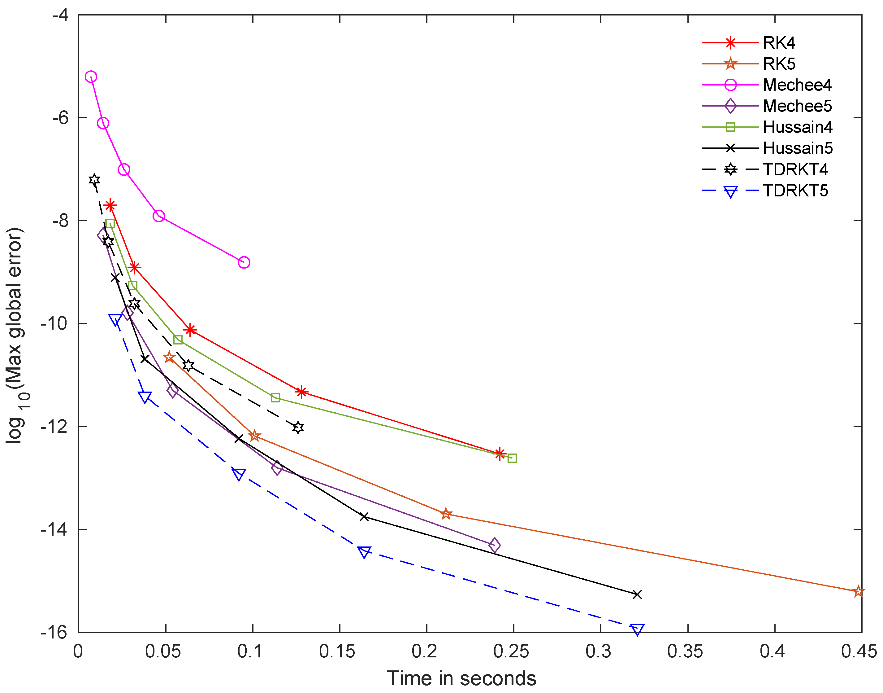
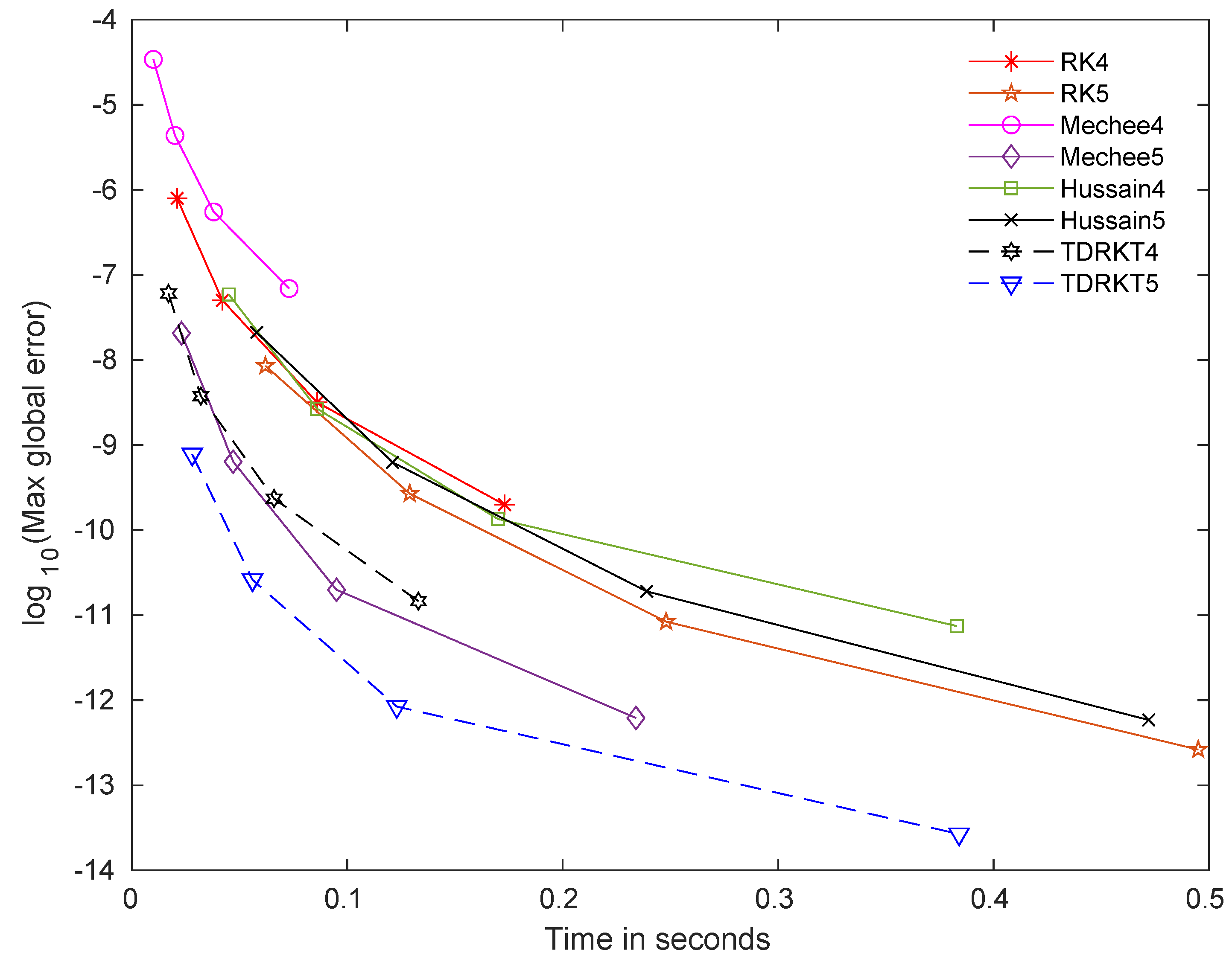
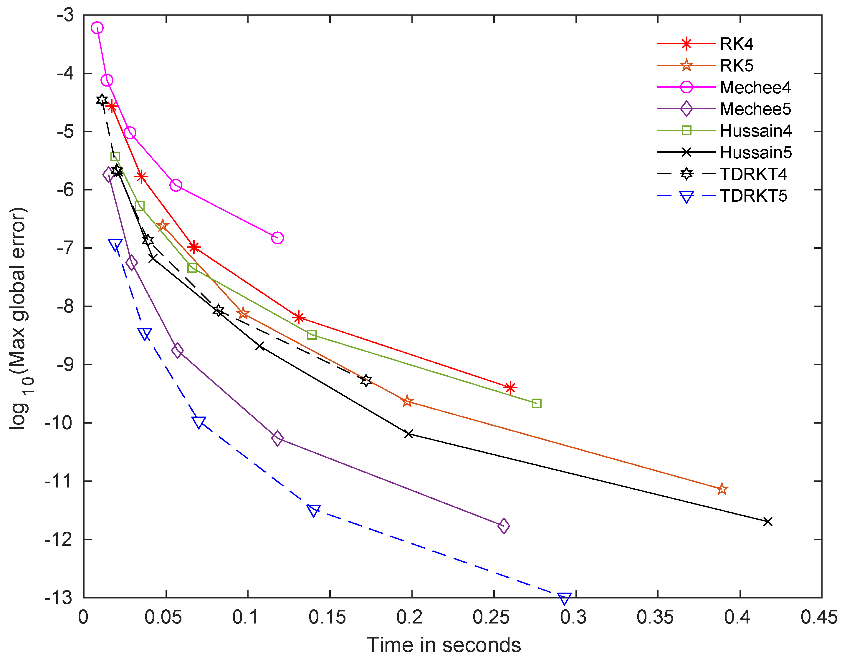
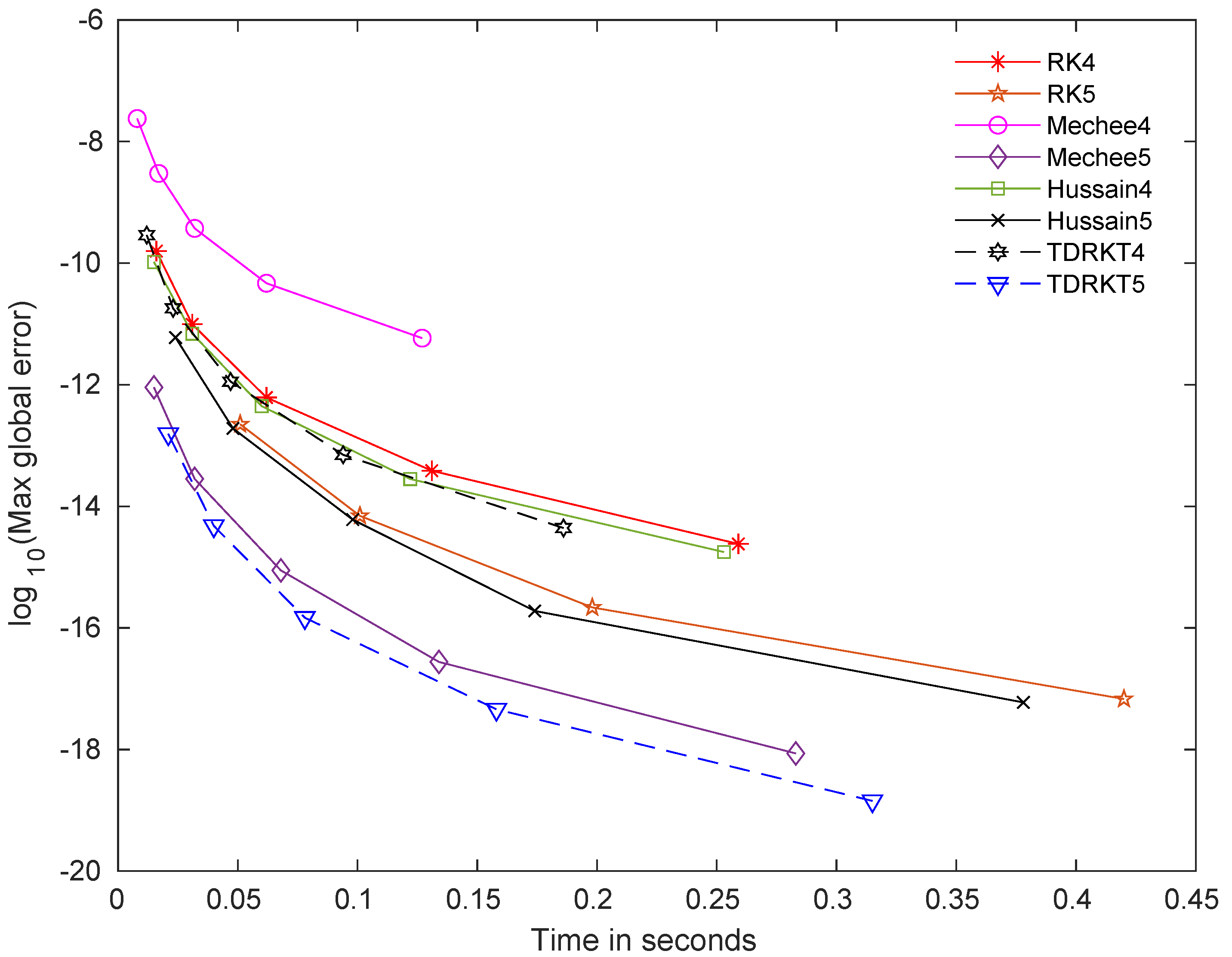
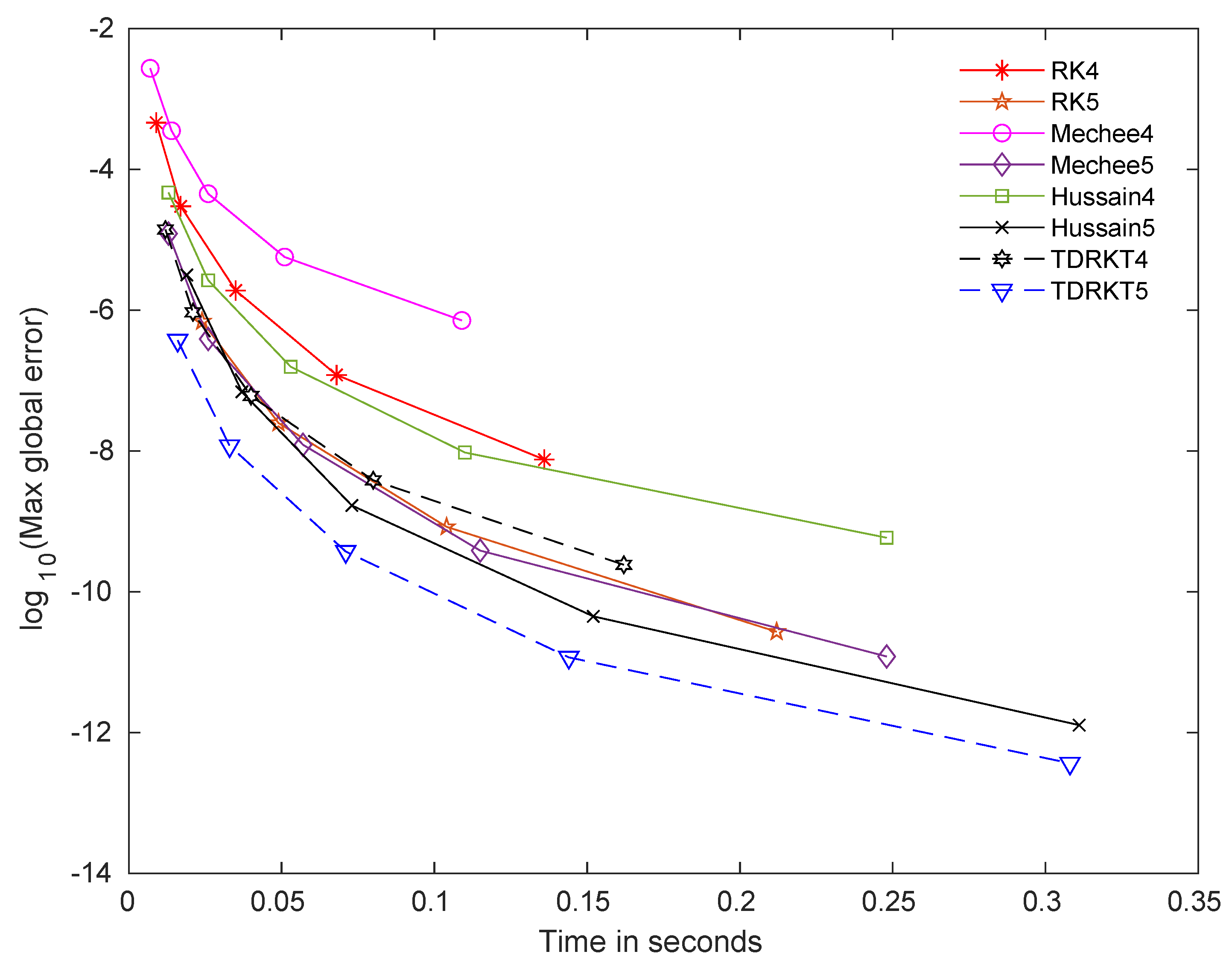
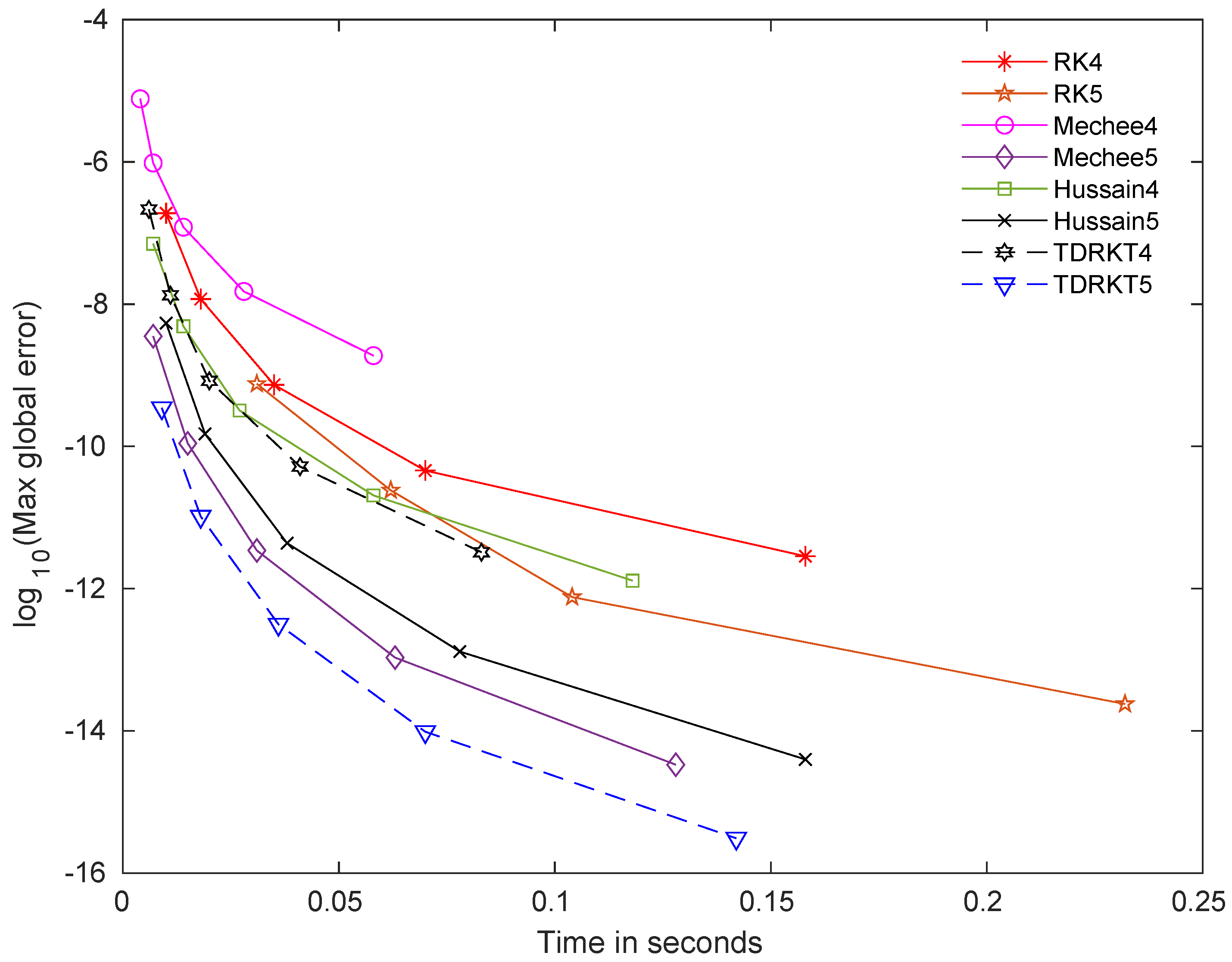
4. Problem Testing and Numerical Result

In this section, we test the efficiency of the new methods with order four and five on selected numerical problems for comparison purpose. Below are the numerical methods utilised to be compared:

• TDRKT4—Explicit two-derivative Runge–Kutta type method with two stage fourth-order.
• TDRKT5—Explicit two-derivative Runge–Kutta type method with three stage fifth-order.
• RK4—Runge–Kutta fourth-order method as given in Hossain et al. [13].
• RK5—Runge–Kutta fifth-order method as given in Goeken and Johnson [14].
• Mechee4—Explicit two stage fourth-order direct method proposed by Mechee et al. [15].
• Mechee5—Explicit three stage fifth-order direct method proposed by Mechee et al. [16].
• Hussain4—Fourth-order improved Runge–Kutta direct method proposed by Hussain et al. [17].
• Hussain5—Fifth-order improved Runge–Kutta direct method proposed by Hussain et al. [18].

Problem 1

Consider the linear homogeneous problem

$$u^{‴}=-u,u\left(0\right)=0,u^{\prime }\left(0\right)=-1,u^{″}\left(0\right)=1,x\in \left[0,5\right]$$

whose analytic solution is $u\left(x\right)=e^{-x}$.

Source: Yap et al. [19]

Problem 2

Consider the nonlinear nonhomogeneous problem

$$u^{‴}=u^2+{(cosx)}^2-cosx-1,u\left(0\right)=0,u^{\prime }\left(0\right)=1,u^{″}\left(0\right)=0,x\in \left[0,5\right]$$

whose analytic solution is $u\left(x\right)=sinx.$

Source: Mechee et al. [16]

Problem 3

Consider the nonlinear homogeneous problem

$$u^{‴}=-6u^4,u\left(0\right)=1,u^{\prime }\left(0\right)=-1,u^{″}\left(0\right)=2,x\in \left[0,5\right]$$

whose analytic solution is $u\left(x\right)=\frac{1}{1+x}.$

Problem 4

Consider the nonlinear homogeneous problem

$$u^{‴}=\frac{3}{8}{u}^{-5},u\left(0\right)=1,u^{\prime }\left(0\right)=\frac{1}{2},u^{″}\left(0\right)=-\frac{1}{4},x\in \left[0,5\right]$$

whose analytic solution is $u\left(x\right)=\sqrt{1+x}.$

Problem 5

Consider linear nonhomogeneous system

$$u_1^{‴}=-u_2-x^2,u_2^{‴}=-u_1+x,$$

$$u_1\left(0\right)=-1,u_1^{\prime }\left(0\right)=0,u_1^{″}\left(0\right)=1,$$

$$u_2\left(0\right)=0,u_2^{\prime }\left(0\right)=1,u_2^{″}\left(0\right)=1,x\in \left[0,1\right]$$

whose analytic solutions are as follows:

$$\begin{array}{c}{u}_1\left(x\right)=x-\frac{5}{6}{e}^x+\frac{1}{2}{e}^{-x}+\frac{1}{3}{e}^{-0.5x}cos\left(\frac{\sqrt{3}}{2}x\right)-e^{0.5x}cos\left(\frac{\sqrt{3}}{2}x\right)+\frac{2\sqrt{3}}{3}{e}^{0.5x}cos\left(\frac{\sqrt{3}}{2}x\right),\hfill \\ u_2\left(x\right)=-x^2+\frac{5}{6}{e}^x+\frac{1}{2}{e}^{-x}-\frac{1}{3}{e}^{-0.5x}cos\left(\frac{\sqrt{3}}{2}x\right)-e^{0.5x}cos\left(\frac{\sqrt{3}}{2}x\right)+\frac{2\sqrt{3}}{3}{e}^{0.5x}cos\left(\frac{\sqrt{3}}{2}x\right).\hfill \end{array}$$

Problem 6

Consider an application nonlinear nonhomogeneous problem, thin film flow of viscous liquid driven by surface tension. In this study, we consider nondimensionalised equation of thin film flow equation as follows:

$$u^{‴}=u^{-3}.$$

(45)

The problem is integrated on the interval $[0,2]$ with the initial conditions $u\left(0\right)=u^{\prime }\left(0\right)=u^{″}\left(0\right)=1$, and this problem can be used to model the draining down of a dry wall of a non-Newtonian thin film (see Momomiat and Mahomed [20]). This equation has no analytical solution (45). Runge–Kutta order 4 method is used to obtain numerical approximation with step size $h=0.0001$ and compare with the selected methods.

5. Numerical Results

Figure 1, Figure 2, Figure 3, Figure 4, Figure 5 and Figure 6 show the numerical performance of selected methods in term of maximum global truncation error versus time of computation. The model of computer used for computing the numerical results is a Lenovo G50-70 Intel Core i3-4030U (1.9 GHz).

Figure 1. Time curves for all methods for problem 1 with $h=\frac{0.05}{2^i},i=0,1,2,3,4$.

Figure 2. Time curves for all methods for problem 2 with $h=\frac{0.05}{2^i},i=0,1,2,3,4$.

Figure 3. Time curves for all methods for problem 3 with $h=\frac{0.05}{2^i},i=0,1,2,3,4$.

Figure 4. Time curves for all methods for problem 4 with $h=\frac{0.0125}{2^i},i=0,1,2,3,4$.

Figure 5. Time curves for all methods for problem 5 with $h=\frac{0.1}{2^i},i=0,1,2,3,4$.

Figure 6. Time curves for all methods for problem 6 with $h=\frac{0.04}{2^i},i=0,1,2,3,4$.

6. Discussion and Conclusions

As a whole, a group of explicit two-derivative Runge–Kutta type TDRKT methods that involve one f-evaluation and multiple g-evaluations for solving initial value problems in the form of $u^{‴}=f(x,u\left(x\right))$ were presented. These newly proposed methods are the extension from special class direct methods for solving $u^{‴}=f(x,u\left(x\right))$, and these methods comprises of algebraic theories of rooted trees and B-series theory referring to the derivation ideas proposed by Butcher [21,22,23] and Chen et al. [6].

In this study, two-stages of order four and three-stages of order five, denoted as TDRKT4 and TDRKT5 methods, are presented based on the algebraic order conditions in the form of $u^{\left(4\right)}=g(x,u\left(x\right),u^{\prime }\left(x\right))$, derivative of $u^{‴}=f(x,u\left(x\right))$ to solve special third-order ODEs directly. The properties of stability, consistency, and convergence for both TDRKT methods are analysed.

The time curves that measured in terms of maximum global error versus time of computation for newly proposed methods and selected methods are displayed in Figure 1, Figure 2, Figure 3, Figure 4, Figure 5 and Figure 6. TDRKT4 and TDRKT5 methods are compared with the selected methods with the same algebraic order, including of RK4, RK5, Mechee4, Mechee5, Hussain4, and Hussain5 methods. In general, even though TDRKT methods have higher cost of computation compared to most existing methods, they acquired much more accurate approximations with the same step size. Maximum global errors of TDRKT methods are lower than that of other existing methods when computational times are similar. TDRKT4 method is more proficient than RK4, Mechee4, and Hussain4 methods; while TDRKT5 method is more efficient compared to RK5, Mechee5, and Hussain5 methods in solving linear homogeneous and nonhomogeneous problems in Figure 1 and Figure 5. Next, TDRKT4 surpasses RK4, Mechee4, and Hussain4 methods and similar to TDRKT5 method, outperforms RK5, Mechee5, and Hussain5 methods in solving both nonlinear homogeneous and nonhomogeneous problems as shown in Figure 2, Figure 3 and Figure 4. In Figure 6, notice that TDRKT4 method is more capable than RK4, Mechee4, and Hussain4 methods; whereas TDRKT5 method is more potent than RK5, Mechee5, and Hussain5 methods in solving application problems with no exact solution, and the numerical approximations are compared to RK4 methods with h = 0.0001.

From the figures above, it is clearly exhibited that TDRKT methods are more proficient than traditional Runge–Kutta methods and direct Runge–Kutta methods in terms of maximum global error versus computational time. TDRKT methods acquired higher accuracy with the same amount of algebraic order compared to traditional Runge–Kutta type methods. Numerical experiments displayed the great performance from TDRKT methods by generating the least maximum global error with the same computational time compared to existing Runge–Kutta type methods.

Following this research, there are several interesting topics that can be explored. Firstly, explicit TDRKT methods can be modified to improved TDRKT methods with the inclusion of parameter $b_{-1}$ and $k_{-i}$ (previous step of $k_i$) in the derivation part. Moreover, TDRKT methods can be enhanced into a hybrid method with symmetry properties or G–symplectic characterisation when applied to time-reversible system. Lastly, TDRKT methods can be adapted to particular types of third-order ODEs such as oscillatory problems. For instance, exponential-fitting or trigonometrically-fitting techniques can be applied to TDRKT methods to make it more effective to solve numerical problems.

References

- Omar, A.A.; Zaer, A.; Ramzi, A.; Shaher, M. A reliable analytical method for solving higher-order initial value problems. Discret. Dyn. Nat. Soc. 2013, 2013, 673829. [Google Scholar]
- Agboola, O.O.; Opanuga, A.A.; Gbadeyan, J.A. Solution of third order ordinary differential equations using differential transform method. Glob. J. Pure Appl. Math. 2015, 11, 2511–2516. [Google Scholar]
- Khataybeh, S.N.; Hashim, I.; Alshbool, M. Solving directly third-order ODEs using operational matrices of Bernstein polynomials method with applications to fluid flow equations. J. King Saud-Univ.-Sci. 2019, 31, 822–826. [Google Scholar] [CrossRef]
- Tang, W.S.; Zhang, J.J. Symmetric integrator based on continuous-stage Runge–Kutta–Nyström methods for reversible systems. Appl. Math. Comput. 2019, 361, 1–12. [Google Scholar] [CrossRef]
- Fang, Y.L.; You, X.; Ming, Q.H. Trigonometrically fitted two-derivative Runge-Kutta methods for solving oscillatory differential equations. Numer. Algorithms 2014, 63, 651–667. [Google Scholar] [CrossRef]
- Chen, Z.; Qiu, Z.; Li, J.; You, X. Two-derivative Runge-Kutta-Nyström methods for second-order ordinary differential equations. Numer. Algorithms 2015, 70, 897–927. [Google Scholar] [CrossRef]
- Ehigie, J.O.; Zou, M.M.; Hou, X.L.; You, X. On modified TDRKN methods for second-order systems of differential equations. Int. J. Comput. Math. 2017, 95, 1–15. [Google Scholar] [CrossRef]
- Mohamed, T.S.; Senu, N.; Ibrahim, Z.B.; Nik Long, N.M.A. Efficient two-derivative Runge-Kutta-Nyström for solving general second-order ordinary differential equations. Discret. Dyn. Nat. Soc. 2018, 2018, 2393015. [Google Scholar] [CrossRef]
- Henrici, P. Discrete Variable Methods in Ordinary Differential Equations; John Wiley & Sons: New York, NY, USA, 1962. [Google Scholar]
- Suli, E.; Mayers, D.F. Discrete Variable Methods in Ordinary Differential Equations; Cambridge University Press: Cambridge, UK, 2003; pp. 337–340. [Google Scholar]
- Lambert, J.D. Numerical Methods for Ordinary Differential Systems: The Initial Value Problem; John Wiley & Sons, Inc.: New York, NY, USA, 1991. [Google Scholar]
- Atkinson, K.; Han, W.; Stewart, D. Numerical Solution of Ordinary Differential Equations: Convergence, Stability and Asymptotic Error; John Wiley & Sons, Inc.: Hoboken, NJ, USA, 2009. [Google Scholar]
- Hossain, B.; Hossain, J.; Miah, M.; Alam, S. A comparative study on fourth order and butcher’s fifth order runge-kutta methods with third order initial value problem (IVP). Appl. Comput. Math. 2017, 6, 243–253. [Google Scholar] [CrossRef]
- Goeken, D.; Johnson, O. Fifth-order Runge-Kutta with higher order derivation approximations. Electron. J. Differ. Equ. 1999, 95, 1–9. [Google Scholar]
- Mechee, M.; Ismail, F.; Siri, Z.; Senu, N. A third-order direct integrators of Runge-Kutta type for special third-order ordinary and delay differential equations. Asian J. Appl. Sci. 2014, 7, 102–116. [Google Scholar] [CrossRef]
- Mechee, M.; Senu, N.; Ismail, F.; Nikouravan, B.; Siri, Z. Three-stage fifth-order Runge-Kutta method for directly solving special third-order differential equation with application to thin film flow problem. Math. Probl. Eng. 2013, 2013, 795397. [Google Scholar] [CrossRef]
- Hussain, K.A.; Ismail, F.; Senu, N.; Rabiei, F. Fourth-order improved Runge–Kutta method for directly solving special third-order ordinary differential equations. Iran. J. Sci. Technol. Trans. Sci. 2017, 41, 429–437. [Google Scholar] [CrossRef]
- Hussain, K.A.; Ismail, F.; Senu, N.; Rabiei, F.; Ibrahim, R. Integration for special third-order ordinary differential equations using improved Runge-Kutta direct method. Malays. J. Sci. 2015, 34, 172–179. [Google Scholar] [CrossRef]
- Yap, L.K.; Ismail, F.; Senu, N. An accurate block hybrid collocation method for third order ordinary differential equations. J. Appl. Math. 2014, 2014, 673829. [Google Scholar] [CrossRef]
- Momoniat, E.; Mahomed, F.M. Symmetry reduction and numerical solution of third-order ode from thin film flow. Math. Comput. Appl. 2015, 15, 709–719. [Google Scholar] [CrossRef]
- Butcher, J.C. Numerical methods for ordinary differential methods in the 20th century. J. Comput. Appl. Math. 2000, 125, 1–29. [Google Scholar] [CrossRef]
- Butcher, J.C. Numerical Methods for Ordinary Differential Equations; John Wiley & Sons: Chichester, UK, 2008. [Google Scholar]
- Butcher, J.C. Trees, stumps, and applications. Axioms 2018, 7, 52. [Google Scholar] [CrossRef]
© 2020 by the authors. Licensee MDPI, Basel, Switzerland. This article is an open access article distributed under the terms and conditions of the Creative Commons Attribution (CC BY) license (http://creativecommons.org/licenses/by/4.0/).