Novel Fractional Operators with Three Orders and Power-Law, Exponential Decay and Mittag–Leffler Memories Involving the Truncated M-Derivative

Abstract

In this research, novel M-truncated fractional derivatives with three orders have been proposed. These operators involve truncated Mittag–Leffler function to generalize the Khalil conformable derivative as well as the M-derivative. The new operators proposed are the convolution of truncated M-derivative with a power law, exponential decay and the complete Mittag–Leffler function. Numerical schemes based on Lagrange interpolation to predict chaotic behaviors of Rucklidge, Shimizu–Morioka and a hybrid strange attractors were considered. Additionally, numerical analysis based on 0–1 test and sensitive dependence on initial conditions were carried out to verify and show the existence of chaos in the chaotic attractor. These results showed that these novel operators involving three orders, two for the truncated M-derivative and one for the fractional term, depict complex chaotic behaviors.

1. Introduction

Fractional calculus, which is a generalization of classical calculus has a wide range in many scientific fields. Fractional order dynamical systems have information about their earlier and present stages to give more realistic information about the dynamical behavior. Therefore, the dynamical behaviors can be conceptualized and explore more accurately in the framework of the fractional derivatives. It is possible to define various integrals and fractional derivatives (non-local or local). Several types of fractional derivatives, with non-local properties have been introduced in the literature, among which we mention Riemann–Liouville, Grünwald–Letnikov, Riesz, Liouville–Caputo, modified Riemann–Liouville, Caputo–Fabrizio and Atangana–Baleanu [1,2].

The local operators are extended from the concept of traditional differentiation. For example, Khalil [3] developed his own derivative which is known as a conformable derivative of order $\alpha$. This operator has the classical properties of the ordinary calculus. Later, Katugampola [4] proposed an alternative fractional derivative similar to the conformable derivative with classical properties, which refers to the Leibniz and Newton calculus. The same author in [5], presented a fractional integral that unifies six fractional integrals: Riemann–Liouville, Hadamard, Erdlyi–Kober, Katugampola, Weyl and Liouville. In 2015, Atangana et al. [6] investigated some properties of Khalil derivative and they introduced some definitions such as q-derivative or fractal derivative. The same author in [7], introduced the Atangana derivative which obeys all the properties satisfied by the Newtonian concept of derivative. Sousa and Oliveira [8] described a derivative that involves the Mittag–Leffler function and it was named M-derivative. More recently, the same authors in [9] introduced a truncated M-derivative, this operator unifies the four existing derivatives above mentioned except the Atangana derivative.

On the other hand, Baleanu et al. [10] proposed a hybrid fractional operator which is expressed as a linear combination of Caputo derivative and the Riemann-Liouville integral. They substituted the classical derivative with the proportional derivative operator defined by Anderson and Ulness [11]. Baleanu et al. found a connection between their operator and the Mittag-Leffler function when they solved differential equations. The aim for which they created this hybrid operator was creating a general operator that allows modeling real data from a range of processes and systems.

This motivation is one of two trends mentioned by Baleanu and Fernandez in [12]. The other is the pure desire to generalize power functions and extend definitions covering different kernel functions. In these work, the authors suggest a classification by organizing fractional operators into classes having different types of properties. One of them, local and non-local operators.

Here, Riemann–Liouville derivative is considered non-local because it does not only depend on the behavior of a function but also on its behavior in a region. Therefore, this is often used in modeling physical processes with memory effects.

In this framework, the non-local (Liouville–Caputo, Caputo–Fabrizio and Atangana–Baleanu) derivatives and local operator based on the truncated M-derivative are considered to propose a generalized operator covering different kernel functions. Therefore, the main contributions of this research are:

• Three order non-local M-fractional derivative with a power law, exponential decay and Mittag–Leffler function.
• Numerical schemes based on Lagrange interpolation to predict chaotic behaviors of Rucklidge, Shimizu–Morioka and a hybrid strange attractor.
• Numerical analysis based on 0–1 test and sensitive dependence on initial conditions to support chaos existence in the above mentioned chaotic attractor.

The paper is organized as follows. Basic definitions and notations of fractional-order derivative are given in Section 2. In Section 3, classical Rucklidge system and Shimizu–Morioka attractor are presented. In Section 4 numerical schemes and chaos analysis for the chaotic attractor are shown. Finally, in Section 5 the conclusions are summarized. The results obtained prove the applicability and validity of these new derivatives and open new investigations and applications in science and engineering.

2. Mathematical Preliminaries

Definition 1.

The Liouville–Caputo operator is the convolution of the local derivative of a given function with a power-law kernel. This derivative of order $(\gamma >0)$ is defined as follows: [1]

$${}_0^C{\mathcal{D}}_t^{\gamma }\left\{f\left(t\right)\right\}=\frac{1}{\Gamma (n-\gamma )}{\int }_0^t\frac{f^{\left(n\right)}\left(\tau \right)}{{(t-\tau )}^{\gamma -n+1}}d\tau ,n-1<\gamma \le n.$$

(1)

Definition 2.

The Caputo–Fabrizio derivative in Liouville–Caputo sense is obtained by replacing the kernel ${(t-\tau )}^{\gamma -n+1}$ with the function $exp\left[-\frac{\gamma }{1-\gamma }t\right]$ and $\frac{1}{\Gamma (1-\gamma )}$ per $\frac{M\left(\gamma \right)}{1-\gamma }$ in the definition (1), then the fractional derivative is defined as [13,14]

$${}_0^{CFC}{\mathcal{D}}_t^{\gamma }\left\{f\left(t\right)\right\}=\frac{M\left(\gamma \right)}{n-\gamma }{\int }_0^t{f}^{\left(n\right)}\left(\tau \right)exp\left[-\frac{\gamma (t-\tau )}{n-\gamma }\right]d\tau ,n-1<\gamma \le n,$$

where $M\left(\gamma \right)$ is a normalization function.

Definition 3.

Let $0<\gamma <1$. The fractional integral of order γ of a function f is defined in [14] as

$${}_0^{CF}{I}_t^{\gamma }\left\{f\left(t\right)\right\}=\frac{2(1-\gamma )}{(2-\gamma )M\left(\gamma \right)}f\left(t\right)+\frac{2\gamma }{(2-\gamma )M\left(\gamma \right)}{\int }_0^{t}f\left(\tau \right)d\tau ,$$

given that the above definition is an average between the function f and its integral of order 1, this implies then that

$$\frac{2(1-\gamma )}{(2-\gamma )M\left(\gamma \right)}+\frac{2\gamma }{(2-\gamma )M\left(\gamma \right)}=1,$$

where,

$$M\left(\gamma \right)=\frac{2}{(2-\gamma )},0\le \gamma \le 1.$$

Definition 4.

Let $f\in H^1(a,b),b>a,\alpha \in [0,1]$ then, the Atangana–Baleanu fractional derivative in Liouville–Caputo sense is given as [2]

$${}_0^{ABC}{\mathcal{D}}_t^{\gamma }\left\{f\left(t\right)\right\}=\frac{AB\left(\gamma \right)}{n-\gamma }{\int }_0^t{f}^{\left(n\right)}\left(\tau \right)E_{\gamma }\left[-\gamma \frac{{(t-\tau )}^{\gamma }}{n-\gamma }\right]d\tau ,n-1<\gamma \le n,$$

where $AB\left(\gamma \right)$ is a normalization function with the same properties as in Caputo–Fabrizio case.

Definition 5.

The fractional integral associate to the Atangana–Baleanu fractional derivative with non-local kernel is defined as

$${}_0^{AB}{I}_t^{\gamma }\left\{f\left(t\right)\right\}=\frac{1-\gamma }{AB\left(\gamma \right)}f\left(t\right)+\frac{\gamma }{AB\left(\gamma \right)\Gamma \left(\gamma \right)}{\int }_0^{t}f\left(\tau \right){(t-\tau )}^{\gamma -1}d\tau ,$$

(2)

when γ is zero we recover the initial function and if also γ is 1, we obtain the ordinary integral.

Definition 6.

Let $f:[0,\infty )\to \mathbb{R}$ and $t>0$. For $0<\alpha <1$ and $\beta >0$, the local M-derivative of f of order α, denoted by ${}_{}^M{\mathcal{D}}_{}^{\alpha ,\beta }$, is defined as below [8]

$${}_{}^M{\mathcal{D}}^{\alpha ,\beta }\left\{f\left(t\right)\right\}=\underset{ϵ\to 0}{lim}\frac{f\left(t{E}_{\beta }\left(ϵt^{-\alpha }\right)\right)-f\left(t\right)}{ϵ}.$$

Definition 7.

Let $f:[0,\infty )\to \mathbb{R}$. For $0<\alpha <1$ and $\beta >0$ a truncated M-fractional derivative of f of order α, denoted by ${}_i^M{\mathcal{D}}_{}^{\alpha ,\beta }$, is defined as below [9]

$${}_i^M{\mathcal{D}}^{\alpha ,\beta }\left\{f\left(t\right)\right\}=\underset{ϵ\to 0}{lim}\frac{f\left(t_i{E}_{\beta }\left(ϵt^{-\alpha }\right)\right)-f\left(t\right)}{ϵ},$$

(3)

$\forall t>0$ and ${}_i{E}_{\beta }(·),\beta >0$ is a truncated Mittag–Leffler function of one parameter defined by Equation (4)

$${}_i{E}_{\beta }\left(z\right)=\sum _{k=0}^i\frac{z^k}{\Gamma (\beta k+1)}.$$

(4)

Some properties of this derivative are presented in the next theorem [15].

Theorem 1.

Let $0<\alpha \le 1$, $\beta >0$ $a,b\in \mathbb{R}$ and f, g α-differentiable at a point $t>0$. Then

1.

${}_i^M{\mathcal{D}}^{\alpha ,\beta }(af+bg)\left(t\right)=a{}_i^M{\mathcal{D}}^{\alpha ,\beta }f\left(t\right)+b{}_i^M{\mathcal{D}}^{\alpha ,\beta }g\left(t\right)$.

2.

${}_i^M{\mathcal{D}}^{\alpha ,\beta }(f·g)\left(t\right)=f\left(t\right){}_i^M{\mathcal{D}}^{\alpha ,\beta }g\left(t\right)+g\left(t\right){}_i^M{\mathcal{D}}^{\alpha ,\beta }f\left(t\right)$.

3.

${}_i^M{\mathcal{D}}^{\alpha ,\beta }\left(\frac{f}{g}\right)\left(t\right)\frac{g\left(t\right){}_i^M{\mathcal{D}}^{\alpha ,\beta }f\left(t\right)-f\left(t\right){}_i^M{\mathcal{D}}^{\alpha ,\beta }g\left(t\right)}{{\left[g\left(t\right)\right]}^2}$.

4.

${}_i^M{\mathcal{D}}^{\alpha ,\beta }\left(c\right)=0$, where $f\left(t\right)=c$ is a constant.

5.

(Chain rule) If f is differentiable, then ${}_i^M{\mathcal{D}}^{\alpha ,\beta }\left\{f\left(t\right)\right\}=\frac{t^{1-\alpha }}{\Gamma (\beta +1)}\frac{df\left(t\right)}{dt}$.

Now, we present three novel operators involving the power law, exponential decay and the complete Mittag–Leffler memory in convolution with the truncated M-derivative.

Definition 8.

Let $y\left(t\right)$ continuous and M-differentiable on $(a,b)$ with order $\alpha ,\beta$, then the M-fractional derivative of f in the Riemann–Liouville sense with order γ is defined as follows

$${}_0^{M-RL}{\mathcal{D}}_t^{\alpha ,\beta ,\gamma }\left\{y\left(t\right)\right\}=\frac{1}{\Gamma (n-\gamma )}{}_i^M{\mathcal{D}}^{\alpha ,\beta }{\int }_0^t\frac{f\left(\tau \right)}{{(t-\tau )}^{\gamma -n+1}}d\tau ,n-1<\alpha ,\gamma \le n,\beta >0,$$

(5)

where ${}_i^M{\mathcal{D}}^{\alpha ,\beta }\left\{y\left(t\right)\right\}=\frac{t^{1-\alpha }}{\Gamma (\beta +1)}\frac{df\left(t\right)}{dt}$ and ${}_i{E}_{\beta }(·),\beta >0$ is the truncated one parameter Mittag–Leffler function defined in Equation (4), $\forall t>0$.

Definition 9.

Let $y\left(t\right)$ continuous and M-differentiable on $(a,b)$ with order $\alpha ,\beta$, then the M-fractional derivative of f in the Caputo–Fabrizio–Riemann–Liouville sense with order γ is defined as follows

$${}_0^{M-CFRL}{\mathcal{D}}_t^{\alpha ,\beta ,\gamma }\left\{y\left(t\right)\right\}=\frac{M\left(\gamma \right)}{n-\gamma }{}_i^M{\mathcal{D}}^{\alpha ,\beta }{\int }_0^{t}f\left(\tau \right)exp\left[-\frac{\gamma (t-\tau )}{n-\gamma }\right]d\tau ,n-1<\alpha ,\gamma \le n,\beta >0,$$

(6)

where ${}_i^M{\mathcal{D}}^{\alpha ,\beta }\left\{y\left(t\right)\right\}$ is defined on property 5 and ${}_i{E}_{\beta }(·),\beta >0$ is defined in Equation (4), $\forall t>0$.

Definition 10.

Let $y\left(t\right)$ continuous and M-differentiable on $(a,b)$ with order $\alpha ,\beta$, then the M-fractional derivative of f in Atangana–Baleanu–Riemann–Liouville sense with order γ is defined as follows

$${}_0^{M-ABRL}{\mathcal{D}}_t^{\alpha ,\beta ,\gamma }\left\{f\left(t\right)\right\}=\frac{AB\left(\gamma \right)}{n-\gamma }{}_i^M{\mathcal{D}}^{\alpha ,\beta }{\int }_0^{t}f\left(\tau \right)E_{\gamma }\left[-\gamma \frac{{(t-\tau )}^{\gamma }}{n-\gamma }\right]d\tau ,n-1<\alpha ,\gamma \le n,\beta >0,$$

(7)

where ${}_i^M{\mathcal{D}}^{\alpha ,\beta }\left\{f\left(t\right)\right\}$ is defined on property 5 and ${}_i{E}_{\beta }(·),\beta >0$ is defined in Equation (4), $\forall t>0$.

In the next section, we consider these novel fractional operators with three orders involving the truncated M-derivative in convolution with the power-law, exponential decay law and Mittag–Leffler kernel given in Equations (5)–(7) to predict complex chaotic behaviors of Rucklidge, Shimizu–Morioka and hybrid strange attractors.

3. Rucklidge, Shimizu–Morioka and Hybrid Strange Attractors

3.1. Rucklidge Attractor

The Rucklidge system [16] is described by using autonomous differential equations as follows

$$\begin{array}{cc}\hfill \dot{x}& =-kx+ay-yz,\hfill \\ \hfill \dot{y}& =x,\hfill \\ \hfill \dot{z}& =-z+y^2,\hfill \end{array}$$

(8)

where a, k are unfolding real parameters; and $x,y,z\in {\mathbb{R}}^3$ are the states. The system (8) was obtained from [17] by using partial differential equations with Galërkin method. Rucklidge model considers the 2D convection problem of Boussinesq fluid.

Figure 1 shows a numerical simulation for Equation (8) with initial conditions: $x\left(0\right)=1$, $y\left(0\right)=0$, $z\left(0\right)=4.5$; parameters of the system: $a=6.7$, $k=2$; simulation time $t=100$ [s] and step size $\Delta t=1\times {10}^{-2}$.

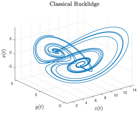
Figure 1. Numerical simulation of the Rucklidge attractor (8) for $a=6.7$, $k=2$; with initial conditions $x\left(0\right)=1$, $y\left(0\right)=0$ and $z\left(0\right)=4.5$.

3.2. Shimizu–Morioka Attractor

Shimizu and Morioka proposed in [18], an algebraic system which exhibits Lorenz-like dynamics. This system is composed by a set of three non-linear differential equations given by

$$\begin{array}{cc}\hfill \dot{x}& =y,\hfill \\ \hfill \dot{y}& =x-By-xz,\hfill \\ \hfill \dot{z}& =-az+x^2,\hfill \end{array}$$

(9)

where $a,B>0$ are the parameters of the system. For some B values, the system above proposed displays a Hopf bifurcation (critical and supercritical). This system has two fixed points, $F_{\pm }$ located at $(\pm \sqrt{\alpha },0,1)$ and one more $F_0$ located at the origin.

Figure 2 shows the numerical result for Equation (9) with initial conditions: $x\left(0\right)=-1$, $y\left(0\right)=2$, $z\left(0\right)=1$; parameters of the system: $a=0.45$, $B=0.75$; simulation time $t=100$ [s] and step size $\Delta t=1\times {10}^{-2}$.

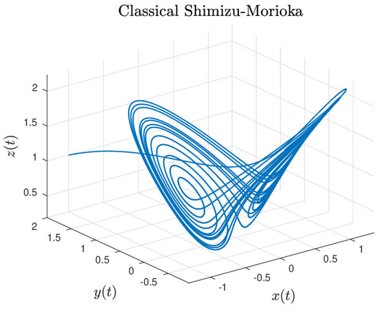
Figure 2. Numerical simulation of Shimizu–Morioka attractor (9) for $a=0.45$, $B=0.75$; with initial conditions $x\left(0\right)=-1$, $y\left(0\right)=2$ and $z\left(0\right)=1$.

3.3. Strange Hybrid Attractor

Sprott in [19] proposed a three-dimensional time-reversible system with quadratic non-linearity and an unusual property that exhibits conservative behavior for some initial conditions and dissipative behavior for another. The conservative behavior has quasi-periodic orbits because the dissipative is chaotic. This strange attractor coexists with an infinite set of nested invariant tori in the state space and it is expressed by the following equations

$$\begin{array}{cc}\hfill \dot{x}& =y+2xy+xz,\hfill \\ \hfill \dot{y}& =1-2x^2+yz,\hfill \\ \hfill \dot{x}& =x-x^2-y^2.\hfill \end{array}$$

(10)

Since the only possible solutions are quasi-periodic or chaotic, the system (10) is bounded with no equilibrium points (stable or unstable).

The dynamic behavior for the strange hybrid attractor is shown in Figure 3, with initial conditions: $x\left(0\right)=2$, $y\left(0\right)=0$, $z\left(0\right)=0$; simulation time $t=100$ [s] and step size $\Delta t=1\times {10}^{-2}$.

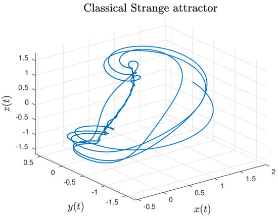
Figure 3. Numerical simulation for strange hybrid attractor (10) with initial conditions $x\left(0\right)=2$, $y\left(0\right)=0$ and $z\left(0\right)=0$.

4. Numerical Schemes and Simulations for Chaotic Attractors

In this section, novel numerical schemes based on the scheme proposed by Toufik and Atangana [20] are proposed to predict chaotic behaviors for the truncated M-Rucklidge, truncated M-Shimizu–Morioka and truncated M-Strange hybrid fractional attractors in Liouville–Caputo, Caputo–Fabrizio and Atangana–Baleanu sense with three orders $\alpha ,\beta ,\gamma$.

4.1. Truncated M-Fractional Rucklidge Attractor with Three Orders and Power-Law, Exponential Decay Law and Mittag–Leffler Memories

Considering the truncated M-derivative (3), the time operators in Equation (8) are generalized by the operator ${}_i^M{\mathcal{D}}^{\alpha ,\beta }$, i.e.,

$$\begin{array}{cc}\hfill {}_i^M{\mathcal{D}}^{\alpha ,\beta }\left\{x\right\}& =-kx+ay-yz,\hfill \\ \hfill {}_i^M{\mathcal{D}}^{\alpha ,\beta }\left\{y\right\}& =x,\hfill \\ \hfill {}_i^M{\mathcal{D}}^{\alpha ,\beta }\left\{z\right\}& =-z+y^2.\hfill \end{array}$$

(11)

By using the property 5 in Theorem 1, the system given in Equation (11) can be written as follows

$$\begin{array}{cc}\hfill {}_i^M{\mathcal{D}}^{\alpha ,\beta }\left\{x\right\}& =\frac{t^{1-\alpha }}{\Gamma (\beta +1)}\left[-kx+ay-yz\right],\hfill \\ \hfill {}_i^M{\mathcal{D}}^{\alpha ,\beta }\left\{y\right\}& =\frac{t^{1-\alpha }}{\Gamma (\beta +1)}\left[x\right],\hfill \\ \hfill {}_i^M{\mathcal{D}}^{\alpha ,\beta }\left\{z\right\}& =\frac{t^{1-\alpha }}{\Gamma (\beta +1)}\left[-z+y^2\right].\hfill \end{array}$$

(12)

The Rucklidge chaotic model given by Equation (8) can be written as follows by using the novel fractional operators with power-law, exponential decay law and Mittag–Leffler kernel in convolution with the truncated M-derivative given in Equations (5)–(7).

• Riemann–Liouville sense

  $$\begin{array}{cc}\hfill {}_0^{M-RL}{\mathcal{D}}_t^{\alpha ,\beta ,\gamma }\left\{x\right\}& =\frac{t^{1-\alpha }}{\Gamma (\beta +1)}f(x,y,z,t),\hfill \\ \hfill {}_0^{M-RL}{\mathcal{D}}_t^{\alpha ,\beta ,\gamma }\left\{y\right\}& =\frac{t^{1-\alpha }}{\Gamma (\beta +1)}g(x,y,z,t),\hfill \\ \hfill {}_0^{M-RL}{\mathcal{D}}_t^{\alpha ,\beta ,\gamma }\left\{z\right\}& =\frac{t^{1-\alpha }}{\Gamma (\beta +1)}h(x,y,z,t).\hfill \end{array}$$

  (13)
• Caputo–Fabrizio sense

  $$\begin{array}{cc}\hfill {}_0^{M-CF}{\mathcal{D}}_t^{\alpha ,\beta ,\gamma }\left\{x\right\}& =\frac{t^{1-\alpha }}{\Gamma (\beta +1)}f(x,y,z,t),\hfill \\ \hfill {}_0^{M-CF}{\mathcal{D}}_t^{\alpha ,\beta ,\gamma }\left\{y\right\}& =\frac{t^{1-\alpha }}{\Gamma (\beta +1)}g(x,y,z,t),\hfill \\ \hfill {}_0^{M-CF}{\mathcal{D}}_t^{\alpha ,\beta ,\gamma }\left\{z\right\}& =\frac{t^{1-\alpha }}{\Gamma (\beta +1)}h(x,y,z,t).\hfill \end{array}$$

  (14)
• Atangana–Baleanu sense

  $$\begin{array}{cc}\hfill {}_0^{M-AB}{\mathcal{D}}_t^{\alpha ,\beta ,\gamma }\left\{x\right\}& =\frac{t^{1-\alpha }}{\Gamma (\beta +1)}f(x,y,z,t),\hfill \\ \hfill {}_0^{M-AB}{\mathcal{D}}_t^{\alpha ,\beta ,\gamma }\left\{y\right\}& =\frac{t^{1-\alpha }}{\Gamma (\beta +1)}g(x,y,z,t),\hfill \\ \hfill {}_0^{M-AB}{\mathcal{D}}_t^{\alpha ,\beta ,\gamma }\left\{z\right\}& =\frac{t^{1-\alpha }}{\Gamma (\beta +1)}h(x,y,z,t).\hfill \end{array}$$

  (15)

where,

$$f(x,y,z,t)=-kx+ay-yz,$$

$$g(x,y,z,t)=x,$$

$$h(x,y,z,t)=-z+y^2.$$

4.1.1. Numerical Scheme for Truncated M-Fractional Rucklidge Attractor in Liouville–Caputo Sense with Three Orders

Equation (13) is converted to the Volterra type since the fractional integral is differentiable, then the Riemann–Liouville derivatives can be replace to Liouville–Caputo derivatives. By applying the Lotka–Volterra integral in both sides of Equation (13), the following equations are obtained [20]

$$\begin{array}{cc}\hfill x\left(t\right)& =x\left(0\right)+\frac{1}{\Gamma \left(\gamma \right)}{\int }_0^t\frac{{\lambda }^{1-\alpha }{\left(t-\lambda \right)}^{\gamma -1}}{\Gamma (\beta +1)}f\left(x,y,z,\lambda \right)d\lambda ,\hfill \\ \hfill y\left(t\right)& =y\left(0\right)+\frac{1}{\Gamma \left(\gamma \right)}{\int }_0^t\frac{{\lambda }^{1-\alpha }{\left(t-\lambda \right)}^{\gamma -1}}{\Gamma (\beta +1)}g\left(x,y,z,\lambda \right)d\lambda ,\hfill \\ \hfill z\left(t\right)& =z\left(0\right)+\frac{1}{\Gamma \left(\gamma \right)}{\int }_0^t\frac{{\lambda }^{1-\alpha }{\left(t-\lambda \right)}^{\gamma -1}}{\Gamma (\beta +1)}h\left(x,y,z,\lambda \right)d\lambda .\hfill \end{array}$$

At a given point $t=t_{n+1},n=0,1,2,\cdots ,$ the above equations are reformulated

$$\begin{array}{cc}\hfill x_{n+1}& =x_0+\frac{1}{\Gamma \left(\gamma \right)}{\int }_0^{t_{n+1}}\frac{{\lambda }^{1-\alpha }{\left(t_{n+1}-\lambda \right)}^{\gamma -1}}{\Gamma (\beta +1)}f\left(x,y,z,\lambda \right)d\lambda ,\hfill \\ \hfill y_{n+1}& =y_0+\frac{1}{\Gamma \left(\gamma \right)}{\int }_0^{t_{n+1}}\frac{{\lambda }^{1-\alpha }{\left(t_{n+1}-\lambda \right)}^{\gamma -1}}{\Gamma (\beta +1)}g\left(x,y,z,\lambda \right)d\lambda ,\hfill \\ \hfill z_{n+1}& =z_0+\frac{1}{\Gamma \left(\gamma \right)}{\int }_0^{t_{n+1}}\frac{{\lambda }^{1-\alpha }{\left(t_{n+1}-\lambda \right)}^{\gamma -1}}{\Gamma (\beta +1)}h\left(x,y,z,\lambda \right)d\lambda .\hfill \end{array}$$

The functions $f\left(x,y,z,\lambda \right)$, $g\left(x,y,z,\lambda \right)$, and $h\left(x,y,z,\lambda \right)$ can be approximated by using the Lagrangian piece-wise interpolation in the following manner

$$\begin{array}{cc}\hfill x_{n+1}& =x_0+\frac{1}{\Gamma \left(\gamma \right)}\sum _{j=0}^n{\int }_{t_j}^{t_{j+1}}\frac{{\lambda }^{1-\alpha }{\left(t_{n+1}-\lambda \right)}^{\gamma -1}}{\Gamma (\beta +1)}f\left(x,y,z,\lambda \right)d\lambda ,\hfill \\ \hfill y_{n+1}& =y_0+\frac{1}{\Gamma \left(\gamma \right)}\sum _{j=0}^n{\int }_{t_j}^{t_{j+1}}\frac{{\lambda }^{1-\alpha }{\left(t_{n+1}-\lambda \right)}^{\gamma -1}}{\Gamma (\beta +1)}g\left(x,y,z,\lambda \right)d\lambda ,\hfill \\ \hfill z_{n+1}& =z_0+\frac{1}{\Gamma \left(\gamma \right)}\sum _{j=0}^n{\int }_{t_j}^{t_{j+1}}\frac{{\lambda }^{1-\alpha }{\left(t_{n+1}-\lambda \right)}^{\gamma -1}}{\Gamma (\beta +1)}h\left(x,y,z,\lambda \right)d\lambda .\hfill \end{array}$$

Finally, in $[t_j,t_{j+1}]$ the following numerical scheme is presented

$$\begin{array}{ll}{x}_{n+1}& =x_0+\frac{{\left(\Delta t\right)}^{\gamma }}{\Gamma (\gamma +2)}{\displaystyle \sum _{j=0}^n}\left[\frac{t_j^{1-\alpha }f\left(x_j,y_j,z_j,t_j\right)}{\Gamma (\beta +1)}({\left(n+1-j\right)}^{\gamma }\left(n-j+2+\gamma \right)-{\left(n-j\right)}^{\gamma }\times \right.\\ & \times \left(n-j+2+2\gamma \right))-\frac{t_{j-1}^{1-\alpha }f\left(x_{j-1},y_{j-1},z_{j-1},t_{j-1}\right)}{\Gamma (\beta +1)}\left({\left(n-j+1\right)}^{\gamma +1}-{\left(n-j\right)}^{\gamma }\left(n-j+1+\gamma \right)\right),\\ y_{n+1}& =y_0+\frac{{\left(\Delta t\right)}^{\gamma }}{\Gamma (\gamma +2)}{\displaystyle \sum _{j=0}^n}\left[\frac{t_j^{1-\alpha }g\left(x_j,y_j,z_j,t_j\right)}{\Gamma (\beta +1)}({\left(n+1-j\right)}^{\gamma }\left(n-j+2+\gamma \right)-{\left(n-j\right)}^{\gamma }\times \right.\\ & \times \left(n-j+2+2\gamma \right))-\frac{t_{j-1}^{1-\alpha }g\left(x_{j-1},y_{j-1},z_{j-1},t_{j-1}\right)}{\Gamma (\beta +1)}\left({\left(n-j+1\right)}^{\gamma +1}-{\left(n-j\right)}^{\gamma }\left(n-j+1+\gamma \right)\right),\\ z_{n+1}& =z_0+\frac{{\left(\Delta t\right)}^{\gamma }}{\Gamma (\gamma +2)}{\displaystyle \sum _{j=0}^n}\left[\frac{t_j^{1-\alpha }h\left(x_j,y_j,z_j,t_j\right)}{\Gamma (\beta +1)}({\left(n+1-j\right)}^{\gamma }\left(n-j+2+\gamma \right)-{\left(n-j\right)}^{\gamma }\times \right.\\ & \times \left(n-j+2+2\gamma \right))-\frac{t_{j-1}^{1-\alpha }h\left(x_{j-1},y_{j-1},z_{j-1},t_{j-1}\right)}{\Gamma (\beta +1)}\left({\left(n-j+1\right)}^{\gamma +1}-{\left(n-j\right)}^{\gamma }\left(n-j+1+\gamma \right)\right).\end{array}$$

(16)

A detailed analysis of the error was shown by Toufik and Atangana in [20].

4.1.2. Numerical Simulations

The numerical results shown in Figure 4 and Figure 5 were carried out by simulating the truncated M-fractional Rucklidge attractor (13) with $\alpha$, $\beta$ and $\gamma$ values arbitrarily chosen. Here, we can get the following cases:

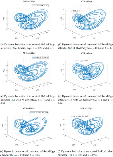
Figure 4. Numerical simulation for truncated M-Rucklidge attractor (12) with initial conditions, $x\left(0\right)=1$, $y\left(0\right)=0$ and $z\left(0\right)=4.5$. Different α and β values were arbitrarily chosen.

Figure 5. Numerical simulation for truncated M-fractional Rucklidge attractor in Liouville–Caputo sense (13) with initial conditions, $x\left(0\right)=1$, $y\left(0\right)=0$ and $z\left(0\right)=4.5$. Different α, β and γ values were arbitrarily chosen.

Case 1.

If $\gamma =1$ in Equation (13), we obtain the truncated M-Rucklidge attractor (12). Figure 4a–f display the numerical approximation for the truncated M-Rucklidge attractor (12) considering the numerical scheme given in Equation (16).

• The Rucklidge attractor of Khalil’s type is recovered when $\alpha \ne 1$ and $\beta =1$, see Figure 4a,b.
• When $\alpha =1$ and $\beta \ne 1$, the M-attractor is showed in Figure 4c,d.
• The behavior of the truncated M-Rucklidge attractor given by Equation (12) is obtained when $\alpha \ne 1$ and $\beta \ne 1$, see Figure 4e,f.

Case 2.

• Now, considering Equation (13), the Rucklidge attractor of Khalil’s type is recovered when $\alpha \ne 1$, $\beta =1$, $\gamma =1$ and $i\to 0$, see Figure 5a.
• If $i\to \infty$, the Katugampola derivative [4] is obtained, since the generalized derivative proposed by Sousa [8] is obtained when $\alpha \ne 1$, $\beta =1$ and $\gamma =1$.
• The Rucklidge attractor involving the M-derivative is shown in Figure 5b. This behavior is obtained when $\alpha =1$, $\beta \ne 1$ and $\gamma =1$.
• The Liouville–Caputo fractional Rucklidge attractor numerical approximation is displayed in Figure 5c with $\alpha =1$, $\beta =1$ and $\gamma \ne 1$.
• By choosing $\alpha \ne 1$, $\beta \ne 1$ and $\gamma =1$, the truncated M-Rucklidge attractor numerical approximation is showed in Figure 5d.

Finally, to carry out the numerical results depicted in Figure 6, the parameters $\alpha \ne 1$, $\beta \ne 1$ and $\gamma \ne 1$ were set to show interesting behaviors. These numerical simulations correspond to the truncated M-fractional Rucklidge attractor in Liouville–Caputo sense with three orders. In these results one can see denser inner rolls in contrast with the classical Rucklidge attractor showed in Figure 1.

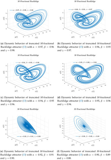
Figure 6. Numerical simulations for truncated M-fractional Rucklidge attractor in Liouville–Caputo sense (13) with initial conditions, $x\left(0\right)=1$, $y\left(0\right)=0$ and $z\left(0\right)=4.5$. Different α, β and γ values were arbitrarily chosen.

The above simulation results were developed for $k=2$ and $a=6.7$; step size $\Delta t=1\times {10}^{-2}$ and simulation time $t=100$ [s], with initial conditions $x\left(0\right)=1,y\left(0\right)=0,z\left(0\right)=4.5$ and different values of α, β and γ arbitrarily chosen.

• Observation. When $\alpha ,\beta ,\gamma \to 1$, the classical Rucklidge attractor is recovered.

4.1.3. Numerical Scheme for Truncated M-Fractional Rucklidge Attractor in Caputo–Fabrizio Sense with Three Orders

The system (13) can be written by applying the Caputo–Fabrizio integral in both sides of these equations

$$\begin{array}{cc}\hfill x\left(t\right)& =x\left(0\right)+\frac{(1-\gamma )t_n^{1-\alpha }}{M\left(\gamma \right)\Gamma (\beta +1)}f(x,y,z,t)+\frac{\gamma }{M\left(\gamma \right)\Gamma (\beta +1)}{\int }_0^t{\lambda }^{1-\alpha }f(x,y,z,\lambda )d\lambda ,\hfill \\ \hfill y\left(t\right)& =y\left(0\right)+\frac{(1-\gamma )t_n^{1-\alpha }}{M\left(\gamma \right)\Gamma (\beta +1)}g(x,y,z,t)+\frac{\gamma }{M\left(\gamma \right)\Gamma (\beta +1)}{\int }_0^t{\lambda }^{1-\alpha }g(x,y,z,\lambda )d\lambda ,\hfill \\ \hfill z\left(t\right)& =z\left(0\right)+\frac{(1-\gamma )t_n^{1-\alpha }}{M\left(\gamma \right)\Gamma (\beta +1)}h(x,y,z,t)+\frac{\gamma }{M\left(\gamma \right)\Gamma (\beta +1)}{\int }_0^t{\lambda }^{1-\alpha }h(x,y,z,\lambda )d\lambda .\hfill \end{array}$$

Reformulating the above-mentioned equations at a given point $t=t_{n+1}$ with $n=0,1,2,\cdots ,N$, we have [20]

$$\begin{array}{cc}\hfill x_{n+1}& =x_n+\frac{(1-\gamma )t_n^{1-\alpha }}{M\left(\gamma \right)\Gamma (\beta +1)}\left\{f(x_n,y_n,z_n,t_n)-f(x_{n-1},y_{n-1},z_{n-1},t_{n-1})\right\}+\hfill \\ \hfill & +\frac{\gamma }{M\left(\gamma \right)\Gamma (\beta +1)}{\int }_{t_n}^{t_{n+1}}{\lambda }^{1-\alpha }f(x,y,z,\lambda )d\lambda ,\hfill \\ \hfill y_{n+1}& =y_n+\frac{(1-\gamma )t_n^{1-\alpha }}{M\left(\gamma \right)\Gamma (\beta +1)}\left\{g(x_n,y_n,z_n,t_n)-g(x_{n-1},y_{n-1},z_{n-1},t_{n-1})\right\}+\hfill \\ \hfill & +\frac{\gamma }{M\left(\gamma \right)\Gamma (\beta +1)}{\int }_{t_n}^{t_{n+1}}{\lambda }^{1-\alpha }g(x,y,z,\lambda )d\lambda ,\hfill \\ \hfill z_{n+1}& =z_n+\frac{(1-\gamma )t_n^{1-\alpha }}{M\left(\gamma \right)\Gamma (\beta +1)}\left\{h(x_n,y_n,z_n,t_n)-h(x_{n-1},y_{n-1},z_{n-1},t_{n-1})\right\}+\hfill \\ \hfill & +\frac{\gamma }{M\left(\gamma \right)\Gamma (\beta +1)}{\int }_{t_n}^{t_{n+1}}{\lambda }^{1-\alpha }h(x,y,z,\lambda )d\lambda .\hfill \end{array}$$

Approximating by the Lagrangian piece-wise interpolation, yields

$$\begin{array}{cc}\hfill x_{n+1}& =x_n+\frac{(1-\gamma )t_n^{1-\alpha }}{M\left(\gamma \right)\Gamma (\beta +1)}\left\{f(x_n,y_n,z_n,t_n)-f(x_{n-1},y_{n-1},z_{n-1},t_{n-1})\right\}+\hfill \\ \hfill & +\frac{\gamma t_{n-1}^{1-\alpha }}{M\left(\gamma \right)\Gamma (\beta +1)}\left[\frac{3(\Delta t)}{2}f(x_n,y_n,z_n,t_n)-\frac{(\Delta t)}{2}f(x_{n-1},y_{n-1},z_{n-1},t_{n-1})\right],\hfill \\ \hfill y_{n+1}& =y_n+\frac{(1-\gamma )t_n^{1-\alpha }}{M\left(\gamma \right)\Gamma (\beta +1)}\left\{g(x_n,y_n,z_n,t_n)-g(x_{n-1},y_{n-1},z_{n-1},t_{n-1})\right\}+\hfill \\ \hfill & +\frac{\gamma t_{n-1}^{1-\alpha }}{M\left(\gamma \right)\Gamma (\beta +1)}\left[\frac{3(\Delta t)}{2}g(x_n,y_n,z_n,t_n)-\frac{(\Delta t)}{2}g(x_{n-1},y_{n-1},z_{n-1},t_{n-1})\right],\hfill \\ \hfill z_{n+1}& =z_n+\frac{(1-\gamma )t_n^{1-\alpha }}{M\left(\gamma \right)\Gamma (\beta +1)}\left\{h(x_n,y_n,z_n,t_n)-h(x_{n-1},y_{n-1},z_{n-1},t_{n-1})\right\}+\hfill \\ \hfill & +\frac{\gamma t_{n-1}^{1-\alpha }}{M\left(\gamma \right)\Gamma (\beta +1)}\left[\frac{3(\Delta t)}{2}h(x_n,y_n,z_n,t_n)-\frac{(\Delta t)}{2}h(x_{n-1},y_{n-1},z_{n-1},t_{n-1})\right].\hfill \end{array}$$

In the interval $[t_j,t_{j+1}]$, we obtain the following numerical scheme

$$\begin{array}{cc}\hfill x_{n+1}& =x_n+\left(\frac{1-\gamma }{M\left(\gamma \right)}+\frac{3\gamma (\Delta t)}{2M\left(\gamma \right)}\right)\frac{t_n^{1-\alpha }f(x_n,y_n,z_n,t_n)}{\Gamma (\beta +1)}-\left(\frac{1-\gamma }{M\left(\gamma \right)}+\frac{\gamma (\Delta t)}{2M\left(\gamma \right)}\right)\times \hfill \\ \hfill & \times \frac{t_{n-1}^{1-\alpha }f(x_{n-1},y_{n-1},z_{n-1},t_{n-1})}{\Gamma (\beta +1)},\hfill \\ \hfill y_{n+1}& =y_n+\left(\frac{1-\gamma }{M\left(\gamma \right)}+\frac{3\gamma (\Delta t)}{2M\left(\gamma \right)}\right)\frac{t_n^{1-\alpha }g(x_n,y_n,z_n,t_n)}{\Gamma (\beta +1)}-\left(\frac{1-\gamma }{M\left(\gamma \right)}+\frac{\gamma (\Delta t)}{2M\left(\gamma \right)}\right)\times \hfill \\ \hfill & \times \frac{t_{n-1}^{1-\alpha }g(x_{n-1},y_{n-1},z_{n-1},t_{n-1})}{\Gamma (\beta +1)},\hfill \\ \hfill z_{n+1}& =z_n+\left(\frac{1-\gamma }{M\left(\gamma \right)}+\frac{3\gamma (\Delta t)}{2M\left(\gamma \right)}\right)\frac{t_n^{1-\alpha }h(x_n,y_n,z_n,t_n)}{\Gamma (\beta +1)}-\left(\frac{1-\gamma }{M\left(\gamma \right)}+\frac{\gamma (\Delta t)}{2M\left(\gamma \right)}\right)\times \hfill \\ \hfill & \times \frac{t_{n-1}^{1-\alpha }h(x_{n-1},y_{n-1},z_{n-1},t_{n-1})}{\Gamma (\beta +1)}.\hfill \end{array}$$

(17)

A detailed analysis of the error was shown by Toufik and Atangana in [20].

4.1.4. Numerical Simulations

In the same way, the truncated M-fractional Rucklidge attractor (14) in Caputo–Fabrizio sense was approximated by the numerical scheme given in Equation (17). The parameters $\alpha \ne 1$, $\beta \ne 1$ and $\gamma \ne 1$ were setting to depict interesting behaviors in Figure 7. In these results, one can see that the states tend to go towards the inner roll in contrast with the truncated M-fractional Rucklidge attractor in the Liouville–Caputo sense.

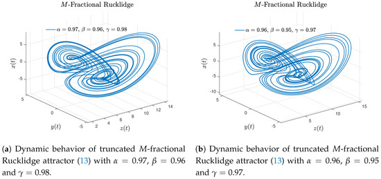
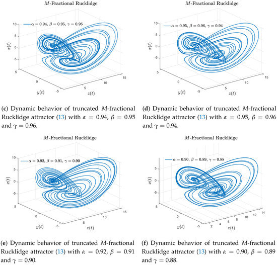
Figure 7. Numerical simulations for truncated M-fractional Rucklidge attractor in Caputo–Fabrizio sense (14) with initial conditions $x\left(0\right)=1$, $y\left(0\right)=0$ and $z\left(0\right)=4.5$. Different $\alpha$, $\beta$ and $\gamma$ values were arbitrarily chosen.

The above approximations were carried out with $k=2$ and $a=6.7$; step size $\Delta t=1\times {10}^{-2}$ and simulation time $t=100$ [s], with initial conditions $x\left(0\right)=1,y\left(0\right)=0,z\left(0\right)=4.5$ by using the parameters $\alpha$, $\beta$ and $\gamma$ arbitrarily chosen.

• Observation. When $\alpha ,\beta ,\gamma \to 1$, the classical Rucklidge attractor is obtained.

4.1.5. Numerical Scheme for Truncated M-Fractional Rucklidge Attractor in Atangana–Baleanu Sense with Three Orders

Applying the Atangana–Baleanu integral (2) in both sides of Equation (15), we get

$$\begin{array}{cc}\hfill x\left(t\right)& =x\left(0\right)+\frac{t^{1-\alpha }(1-\gamma )}{\Gamma (\beta +1)AB\left(\gamma \right)}f(x,y,z,t)+\frac{\gamma t^{1-\alpha }}{AB\left(\gamma \right)\Gamma \left(\gamma \right)}{\int }_0^t\frac{{(t-\lambda )}^{\gamma -1}}{\Gamma (\beta +1)}f(x,y,z,\lambda )d\lambda ,\hfill \\ \hfill y\left(t\right)& =y\left(0\right)+\frac{t^{1-\alpha }(1-\gamma )}{\Gamma (\beta +1)AB\left(\gamma \right)}g(x,y,z,t)+\frac{\gamma t^{1-\alpha }}{AB\left(\gamma \right)\Gamma \left(\gamma \right)}{\int }_0^t\frac{{(t-\lambda )}^{\gamma -1}}{\Gamma (\beta +1)}g(x,y,z,\lambda )d\lambda ,\hfill \\ \hfill z\left(t\right)& =z\left(0\right)+\frac{t^{1-\alpha }(1-\gamma )}{\Gamma (\beta +1)AB\left(\gamma \right)}h(x,y,z,t)+\frac{\gamma t^{1-\alpha }}{AB\left(\gamma \right)\Gamma \left(\gamma \right)}{\int }_0^t\frac{{(t-\lambda )}^{\gamma -1}}{\Gamma (\beta +1)}h(x,y,z,\lambda )d\lambda .\hfill \end{array}$$

In order to use $t_{n+1}$, the following expressions are gotten [20]

$$\begin{array}{cc}\hfill x_{n+1}& =x_0+\frac{t_n^{1-\alpha }(1-\gamma )}{\Gamma (\beta +1)AB\left(\gamma \right)}f(x_n,y_n,z_n,t_n)+\frac{\gamma }{AB\left(\gamma \right)\Gamma \left(\gamma \right)}{\int }_0^{t_{n+1}}\frac{{\lambda }^{1-\alpha }{(t_{n+1}-\lambda )}^{\gamma -1}}{\Gamma (\beta +1)}f(x,y,z,\lambda )d\lambda ,\hfill \\ \hfill y_{n+1}& =y_0+\frac{t_n^{1-\alpha }(1-\gamma )}{\Gamma (\beta +1)AB\left(\gamma \right)}g(x_n,y_n,z_n,t_n)+\frac{\gamma }{AB\left(\gamma \right)\Gamma \left(\gamma \right)}{\int }_0^{t_{n+1}}\frac{{\lambda }^{1-\alpha }{(t_{n+1}-\lambda )}^{\gamma -1}}{\Gamma (\beta +1)}g(x,y,z,\lambda )d\lambda ,\hfill \\ \hfill z_{n+1}& =z_0+\frac{t_n^{1-\alpha }(1-\gamma )}{\Gamma (\beta +1)AB\left(\gamma \right)}h(x_n,y_n,z_n,t_n)+\frac{\gamma }{AB\left(\gamma \right)\Gamma \left(\gamma \right)}{\int }_0^{t_{n+1}}\frac{{\lambda }^{1-\alpha }{(t_{n+1}-\lambda )}^{\gamma -1}}{\Gamma (\beta +1)}h(x,y,z,\lambda )d\lambda .\hfill \end{array}$$

Approximating the integrals by using the Lagrangian piece-wise interpolation, the above equations are expressed as

$$\begin{array}{cc}\hfill x_{n+1}& =x_0+\frac{t_n^{1-\alpha }(1-\gamma )}{\Gamma (\beta +1)AB\left(\gamma \right)}f(x_n,y_n,z_n,t_n)+\frac{\gamma }{AB\left(\gamma \right)\Gamma \left(\gamma \right)}\sum _{j=0}^n{\int }_{t_j}^{t_{j+1}}\frac{{\lambda }^{1-\alpha }{(t_{n+1}-\lambda )}^{\gamma -1}}{\Gamma (\beta +1)}f(x,y,z,\lambda )d\lambda ,\hfill \\ \hfill y_{n+1}& =y_0+\frac{t_n^{1-\alpha }(1-\gamma )}{\Gamma (\beta +1)AB\left(\gamma \right)}g(x_n,y_n,z_n,t_n)+\frac{\gamma }{AB\left(\gamma \right)\Gamma \left(\gamma \right)}\sum _{j=0}^n{\int }_{t_j}^{t_{j+1}}\frac{{\lambda }^{1-\alpha }{(t_{n+1}-\lambda )}^{\gamma -1}}{\Gamma (\beta +1)}g(x,y,z,\lambda )d\lambda ,\hfill \\ \hfill z_{n+1}& =z_0+\frac{t_n^{1-\alpha }(1-\gamma )}{\Gamma (\beta +1)AB\left(\gamma \right)}h(x_n,y_n,z_n,t_n)+\frac{\gamma }{AB\left(\gamma \right)\Gamma \left(\gamma \right)}\sum _{j=0}^n{\int }_{t_j}^{t_{j+1}}\frac{{\lambda }^{1-\alpha }{(t_{n+1}-\lambda )}^{\gamma -1}}{\Gamma (\beta +1)}h(x,y,z,\lambda )d\lambda .\hfill \end{array}$$

Finally, approximating $\frac{1}{\Gamma (\beta +1)}f(x,y,z,t)$, $\frac{1}{\Gamma (\beta +1)}g(x,y,z,t)$ and $\frac{1}{\Gamma (\beta +1)}h(x,y,z,t)$ in $[t_j,t_{j+1}]$, the following numerical scheme is obtained

$$\begin{array}{ll}{x}_{n+1}& =x_0+\frac{t_n^{1-\alpha }(1-\gamma )}{\Gamma (\beta +1)AB\left(\gamma \right)}f(x_n,y_n,z_n,t_n)+\frac{\gamma {(\Delta t)}^{\gamma }}{AB\left(\gamma \right)\Gamma \left(\gamma \right)}{\displaystyle \sum _{j=0}^n}\left[\frac{t_j^{1-\alpha }f(x_j,y_j,z_j,t_j)}{\Gamma (\beta +1)}\right({(n+1-j)}^{\gamma }\times \\ & \times (n-j+2+\gamma )-{(n-j)}^{\gamma }(n-j+2+2\gamma ))-\frac{t_{j-1}^{1-\alpha }f(x_{j-1},y_{j-1},z_{j-1},t_{j-1})}{\Gamma (\beta +1)}({(n-j+1)}^{\gamma +1}-\\ & -{(n-j)}^{\gamma }(n-j+1+\gamma )\left)\right],\\ y_{n+1}& =y_0+\frac{t_n^{1-\alpha }(1-\gamma )}{\Gamma (\beta +1)AB\left(\gamma \right)}g(x_n,y_n,z_n,t_n)+\frac{\gamma {(\Delta t)}^{\gamma }}{AB\left(\gamma \right)\Gamma \left(\gamma \right)}{\displaystyle \sum _{j=0}^n}\left[\frac{t_j^{1-\alpha }g(x_j,y_j,z_j,t_j)}{\Gamma (\beta +1)}\right({(n+1-j)}^{\gamma }\times \\ & \times (n-j+2+\gamma )-{(n-j)}^{\gamma }(n-j+2+2\gamma ))-\frac{t_{j-1}^{1-\alpha }g(x_{j-1},y_{j-1},z_{j-1},t_{j-1})}{\Gamma (\beta +1)}({(n-j+1)}^{\gamma +1}-\\ & -{(n-j)}^{\gamma }(n-j+1+\gamma )\left)\right],\\ z_{n+1}& =z_0+\frac{t_n^{1-\alpha }(1-\gamma )}{\Gamma (\beta +1)AB\left(\gamma \right)}h(x_n,y_n,z_n,t_n)+\frac{\gamma {(\Delta t)}^{\gamma }}{AB\left(\gamma \right)\Gamma \left(\gamma \right)}{\displaystyle \sum _{j=0}^n}\left[\frac{t_j^{1-\alpha }h(x_j,y_j,z_j,t_j)}{\Gamma (\beta +1)}\right({(n+1-j)}^{\gamma }\times \\ & \times (n-j+2+\gamma )-{(n-j)}^{\gamma }(n-j+2+2\gamma ))-\frac{t_{j-1}^{1-\alpha }h(x_{j-1},y_{j-1},z_{j-1},t_{j-1})}{\Gamma (\beta +1)}({(n-j+1)}^{\gamma +1}-\\ & -{(n-j)}^{\gamma }(n-j+1+\gamma )\left)\right].\end{array}$$

(18)

A detailed analysis of the error was shown by Toufik and Atangana in [20].

4.1.6. Numerical Simulations

The numerical simulations given in Figure 8, shown new behaviors for the truncated M-fractional Rucklidge attractor with Mittag–Leffler memory considering $\alpha \ne 1$, $\beta \ne 1$ and $\gamma \ne 1$. These behaviors depict attractor Rucklidge-like without an inner double roll.

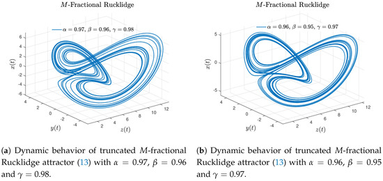
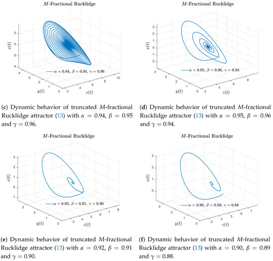
Figure 8. Numerical simulations for truncated M-fractional Rucklidge attractor in Atangana–Baleanu–Caputo sense (15) with initial conditions $x\left(0\right)=1$, $y\left(0\right)=0$ and $z\left(0\right)=4.5$. Different $\alpha$, $\beta$ and $\gamma$ values were arbitrarily chosen.

All simulations referred above were developed for $k=2$ and $a=6.7$; step size $\Delta t=1\times {10}^{-2}$ and simulation time $t=100$ [s], with initial conditions $x\left(0\right)=1,y\left(0\right)=0,z\left(0\right)=4.5$ by considering different cases of $\alpha$, $\beta$ and $\gamma$ arbitrarily chosen.

• Observation. When $\alpha ,\beta ,\gamma \to 1$, the classical Rucklidge attractor is recovered.

4.1.7. Chaos Analysis

The 0-1 test is a chaos analysis which provides a 2-dimensional system. This system, from $\varphi \left(t\right)$ for $t=1,2,\cdots ,T$, is given as

$$\begin{array}{cc}\hfill p(t+1)& =p\left(t\right)+\varphi (t+1)cos\left(cn\right),\hfill \\ \hfill q(t+1)& =q\left(t\right)+\varphi (t+1)sin\left(cn\right),\hfill \end{array}$$

where c is fixed as $c\in (0,2\pi )$.

For a continuous time system, the 2-dimensional mean square displacement is given as follows

$$M_c\left(t\right)=\underset{T\to \infty }{lim}\frac{1}{T}{\int }_0^T\left({\left[p(t+\tau )-p\left(\tau \right)\right]}^2+{\left[q(t+\tau )-q\left(\tau \right)\right]}^2\right)d\tau ,$$

(19)

where the growth rate is defined as

$$K=\underset{t\to \infty }{lim}\frac{log\left(M_c\left(t\right)\right)}{log\left(t\right)}.$$

If $K\approx 0$ then it means that the system is regular, on the other hand, the system is chaotic if $K\approx 1$ [21].

Here, Equation (19) is approximated by a time series sampled with a sampled time ${\tau }_s$

$$M_c\left(n\right)=\underset{N\to \infty }{lim}\frac{1}{N}\sum _{j=1}^N\left({\left[p_{{\tau }_s}(j+n)-p_{{\tau }_s}\left(j\right)\right]}^2+{\left[q_{{\tau }_s}(j+n)-q_{{\tau }_s}\left(j\right)\right]}^2\right){\tau }_s^2.$$

(20)

This test is applied with ${\tau }_s=0.0156$ in order to analyze the present chaos in the M-Rucklidge attractor. Table 1 shows the growth rates by using the operators given by Equations (13)–(15). In general, one can conclude that the dynamic in each state is chaotic.

Table 1. Growth rates for M-fractional Rucklidge attractor.

Derivative	${\mathit{x}}_1$	${\mathit{x}}_2$	${\mathit{x}}_3$
M–Liouville–Caputo	0.9557	0.8915	0.9308
M–Caputo–Fabrizio	0.9960	0.9796	0.9541
M–Atangana–Baleanu	0.9926	0.9668	0.9358

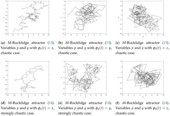
Figure 9 depicts typical plots of p and q for chaotic dynamics. This figure illustrates a strong chaotic dynamic in state x for M-fractional Rucklidge attractor in Caputo–Fabrizio and Atangana–Baleanu sense. In addition, contrasting behaviors of the variables p and q is shown.

Figure 9. Variables p and q in Rucklidge attractor (23) by using M–Liouville–Caputo (5), M–Caputo–Fabrizio (6) and M–Atangana–Baleanu (7) derivatives, respectively.

4.2. Truncated M-Fractional-Shimizu–Morioka Attractor with Three Orders and Mittag–Leffler Memory

Considering Equation (7), the Shimizu–Morioka system (9) is written as follows

$$\begin{array}{cc}\hfill {}_0^{M-AB}{\mathcal{D}}_t^{\alpha ,\beta ,\gamma }\left(x\right)& =\frac{t^{1-\alpha }}{\Gamma (\beta +1)}\left[y\right],\hfill \\ \hfill {}_0^{M-AB}{\mathcal{D}}_t^{\alpha ,\beta ,\gamma }\left(y\right)& =\frac{t^{1-\alpha }}{\Gamma (\beta +1)}\left[x-By-xz\right],\hfill \\ \hfill {}_0^{M-AB}{\mathcal{D}}_t^{\alpha ,\beta ,\gamma }\left(z\right)& =\frac{t^{1-\alpha }}{\Gamma (\beta +1)}\left[-az+x^2\right],\hfill \end{array}$$

(21)

based on the numerical scheme formulated in Equation (18), we get

$$\begin{array}{cc}\hfill x_{n+1}& =x_0+\frac{t_n^{1-\alpha }(1-\gamma )}{\Gamma (\beta +1)AB\left(\gamma \right)}{y}_n+\frac{\gamma t_n^{1-\alpha }{(\Delta t)}^{\gamma }}{AB\left(\gamma \right)\Gamma \left(\gamma \right)}\sum _{j=0}^n\left[\frac{y_j}{\Gamma (\beta +1)}\right({(n+1-j)}^{\gamma }(n-j+2+\gamma )-\hfill \\ \hfill & -{(n-j)}^{\gamma }(n-j+2+2\gamma ))-\frac{y_{j-1}}{\Gamma (\beta +1)}\left({(n-j+1)}^{\gamma +1}-{(n-j)}^{\gamma }(n-j+1+\gamma )\right)],\hfill \\ \hfill y_{n+1}& =y_0+\frac{t_n^{1-\alpha }(1-\gamma )}{\Gamma (\beta +1)AB\left(\gamma \right)}\left(x_n-B{y}_n-x_n{z}_n\right)+\frac{\gamma t_n^{1-\alpha }{(\Delta t)}^{\gamma }}{AB\left(\gamma \right)\Gamma \left(\gamma \right)}\sum _{j=0}^n\left[\frac{\left(x_j-B{y}_j-x_j{z}_j\right)}{\Gamma (\beta +1)}\right({(n+1-j)}^{\gamma }\times \hfill \\ \hfill & \times (n-j+2+\gamma )-{(n-j)}^{\gamma }(n-j+2+2\gamma ))-\frac{\left(x_{j-1}-B{y}_{j-1}-x_{j-1}{z}_{j-1}\right)}{\Gamma (\beta +1)}({(n-j+1)}^{\gamma +1}-\hfill \\ \hfill & -{(n-j)}^{\gamma }(n-j+1+\gamma )\left)\right],\hfill \\ \hfill z_{n+1}& =z_0+\frac{t_n^{1-\alpha }(1-\gamma )}{\Gamma (\beta +1)AB\left(\gamma \right)}\left(-a{z}_n+x_n^2\right)+\frac{\gamma t_n^{1-\alpha }{(\Delta t)}^{\gamma }}{AB\left(\gamma \right)\Gamma \left(\gamma \right)}\sum _{j=0}^n\left[\frac{\left(-a{z}_j+x_j^2\right)}{\Gamma (\beta +1)}\right({(n+1-j)}^{\gamma }\times \hfill \\ \hfill & \times (n-j+2+\gamma )-{(n-j)}^{\gamma }(n-j+2+2\gamma ))-\frac{\left(-a{z}_{j-1}+x_{j-1}^2\right)}{\Gamma (\beta +1)}({(n-j+1)}^{\gamma +1}-\hfill \\ \hfill & -{(n-j)}^{\gamma }(n-j+1+\gamma )\left)\right].\hfill \end{array}$$

(22)

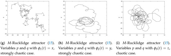
The numerical results shown in Figure 10 and Figure 11 were carried out by simulating the truncated M-fractional Shimizu–Morioka attractor with Mitagg-Leffler memory (21) with $\alpha$, $\beta$ and $\gamma$ values arbitrarily chosen.

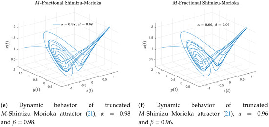
Figure 10. Numerical simulation for truncated M-Shimizu–Morioka attractor (21) with initial conditions $x\left(0\right)=-1$, $y\left(0\right)=2$ and $z\left(0\right)=1$. Different $\alpha$, $\beta$ and $\gamma$ values were arbitrarily chosen.

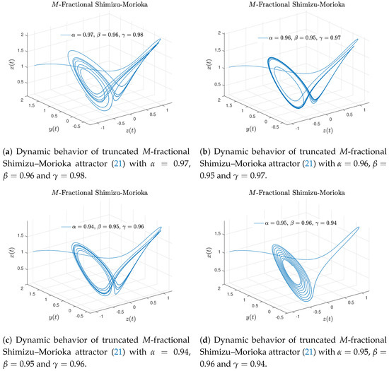
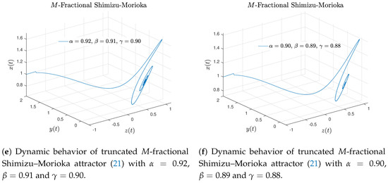
Figure 11. Numerical simulations for truncated M-fractional Shimizu–Morioka attractor in Atangana–Baleanu–Caputo sense (21) with initial conditions $x\left(0\right)=-1$, $y\left(0\right)=2$, $z\left(0\right)=1$. Different $\alpha$, $\beta$ and $\gamma$ values were arbitrarily chosen.

If $\gamma =1$ in Equation (21), we get the truncated M-Rucklidge attractor. Figure 10a–f display the numerical approximation for the truncated M-Shimizu–Morioka attractor considering the numerical scheme shown in Equation (22).

• The Shimizu–Morioka attractor of Khalil’s type is recovered when $\alpha \ne 1$ and $\beta =1$, see Figure 10a,b.
• When $\alpha =1$ and $\beta \ne 1$, the M-derivative Shimizu–Morioka attractor is showed in Figure 10c,d.
• The behavior of the truncated M-Shimizu–Morioka attractor is obtained when $\alpha \ne 1$ and $\beta \ne 1$, see Figure 10e,f.

By setting $a=0.45$ and $B=0.75$; with initial conditions $x\left(0\right)=-1$, $y\left(0\right)=2$, $z\left(0\right)=1$, step size $\Delta t=1\times {10}^{-2}$ and simulation time $t=100$ [s] numerical simulations for the truncated M-fractional Shimizu–Morioka attractor (21) of order $\alpha$, $\beta$ and $\gamma$ are presented in Figure 11. Although inner rolls are not present, symmetry still remains. This is because the Mittag–Leffler function present in the Atangana–Baleanu formulation describes the memory effect better than other fractional operators.

• Observation. When $\alpha ,\beta ,\gamma \to 1$, the classical Shimizu–Morioka attractor is obtained.

Chaos Analysis

In the same way, M-fractional Shimizu–Morioka attractor in Atangana–Baleanu sense (21) is analyzed by using the 2-dimensional mean square displacement approximation (20) to verify the existence of chaos. According to the results shown in Table 2, the chaos existence is strongly present in states $x_2$ and $x_3$. It can be seen in Figure 12.

Table 2. Growth rates for M-Shimizu–Morioka attractor (21).

Derivative	${\mathit{x}}_1$	${\mathit{x}}_2$	${\mathit{x}}_3$
M–Atangana–Baleanu	0.9676	0.9908	0.9900

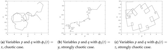
Figure 12. Variables p and q in M-Shimizu–Morioka attractor (21) by using M–Atangana–Baleanu (7).

4.3. Truncated M-Fractional Strange Hybrid Attractor with Three Orders and Mittag–Leffler Memory

Each state of the model (10) is generalized by using the truncated M-fractional operator in Atangana–Baleanu sense (7). In this example, we consider the incommensurate strange hybrid attractor with nine non-integer orders to generate novel behaviors with different dynamics. As particular cases, each state would have the derivative of Khalil [3], Katugampola [4], Sousa and Oliveira [8], the fractional derivative of Atangana–Baleanu [2] or a combination of them. The incommensurate truncated M-fractional strange hybrid attractor is given by

$$\begin{array}{cc}\hfill {}_0^{M-AB}{\mathcal{D}}_t^{{\alpha }_1,{\beta }_1,{\gamma }_1}\left(x\right)& =\frac{t^{1-{\alpha }_1}}{\Gamma ({\beta }_1+1)}\left[y+2xy+xz\right],\hfill \\ \hfill {}_0^{M-AB}{\mathcal{D}}_t^{{\alpha }_2,{\beta }_2,{\gamma }_2}\left(y\right)& =\frac{t^{1-{\alpha }_2}}{\Gamma ({\beta }_2+1)}\left[1-2x^2+yz\right],\hfill \\ \hfill {}_0^{M-AB}{\mathcal{D}}_t^{{\alpha }_3,{\beta }_3,{\gamma }_3}\left(z\right)& =\frac{t^{1-{\alpha }_3}}{\Gamma ({\beta }_3+1)}\left[x-x^2-y^2\right].\hfill \end{array}$$

(23)

The numerical approximation of the strange hybrid model given by Equation (23) derives from the numerical scheme developed in Equation (18) and it is expressed as follows

$$\begin{array}{cc}\hfill x_{n+1}& =x_0+\frac{t_n^{1-{\alpha }_1}(1-{\gamma }_1)}{\Gamma ({\beta }_1+1)AB\left({\gamma }_1\right)}f(x_n,y_n,z_n,t_n)+\frac{{\gamma }_1{t}_n^{1-{\alpha }_1}{(\Delta t)}^{{\gamma }_1}}{AB\left({\gamma }_1\right)\Gamma \left({\gamma }_1\right)}\sum _{j=0}^n\left[\frac{f(x_j,y_j,z_j,t_j)}{\Gamma ({\beta }_1+1)}\right({(n+1-j)}^{{\gamma }_1}\times \hfill \\ \hfill & \times (n-j+2+{\gamma }_1)-{(n-j)}^{{\gamma }_1}(n-j+2+2{\gamma }_1))-\frac{f(x_{j-1},y_{j-1},z_{j-1},t_{j-1})}{\Gamma ({\beta }_1+1)}({(n-j+1)}^{{\gamma }_1+1}-\hfill \\ \hfill & -{(n-j)}^{{\gamma }_1}(n-j+1+{\gamma }_1)\left)\right],\hfill \\ \hfill y_{n+1}& =y_0+\frac{t_n^{1-{\alpha }_2}(1-{\gamma }_2)}{\Gamma ({\beta }_2+1)AB\left({\gamma }_2\right)}g(x_n,y_n,z_n,t_n)+\frac{{\gamma }_2{t}_n^{1-{\alpha }_2}{(\Delta t)}^{{\gamma }_2}}{AB\left({\gamma }_2\right)\Gamma \left({\gamma }_2\right)}\sum _{j=0}^n\left[\frac{g(x_j,y_j,z_j,t_j)}{\Gamma ({\beta }_2+1)}\right({(n+1-j)}^{{\gamma }_2}\times \hfill \\ \hfill & \times (n-j+2+{\gamma }_2)-{(n-j)}^{{\gamma }_2}(n-j+2+2{\gamma }_2))-\frac{g(x_{j-1},y_{j-1},z_{j-1},t_{j-1})}{\Gamma ({\beta }_2+1)}({(n-j+1)}^{{\gamma }_2+1}-\hfill \\ \hfill & -{(n-j)}^{{\gamma }_2}(n-j+1+{\gamma }_2)\left)\right],\hfill \\ \hfill z_{n+1}& =z_0+\frac{t_n^{1-{\alpha }_3}(1-{\gamma }_3)}{\Gamma ({\beta }_3+1)AB\left({\gamma }_3\right)}h(x_n,y_n,z_n,t_n)+\frac{{\gamma }_3{t}_n^{1-{\alpha }_3}{(\Delta t)}^{{\gamma }_3}}{AB\left({\gamma }_3\right)\Gamma \left({\gamma }_3\right)}\sum _{j=0}^n\left[\frac{h(x_j,y_j,z_j,t_j)}{\Gamma ({\beta }_3+1)}\right({(n+1-j)}^{{\gamma }_3}\times \hfill \\ \hfill & \times (n-j+2+{\gamma }_3)-{(n-j)}^{{\gamma }_3}(n-j+2+2{\gamma }_3))-\frac{h(x_{j-1},y_{j-1},z_{j-1},t_{j-1})}{\Gamma ({\beta }_3+1)}({(n-j+1)}^{{\gamma }_3+1}-\hfill \\ \hfill & -{(n-j)}^{{\gamma }_3}(n-j+1+{\gamma }_3)\left)\right],\hfill \end{array}$$

where,

$$f(x,y,z,t)=y+2xy+xz,$$

$$g(x,y,z,t)=1-2x^2+yz,$$

$$h(x,y,z,t)=x-x^2-y^2.$$

Now, we consider several numerical simulations choosing arbitrarily values for the parameters ${\alpha }_i$, ${\beta }_i$ and ${\gamma }_i$ as follows:

Case 1.

Choosing ${\alpha }_1=0.98$, ${\beta }_1=0.97$, ${\gamma }_1=0.96$ for the state x; ${\alpha }_2=0.96$, ${\beta }_2=0.97$, ${\gamma }_2=1$ for the state y; and ${\alpha }_3=1$, ${\beta }_3=1$, ${\gamma }_3=0.97$ for the state z; Figure 13a shows interesting behavior for the truncated M-fractional strange hybrid attractor in Atangana–Baleanu sense.

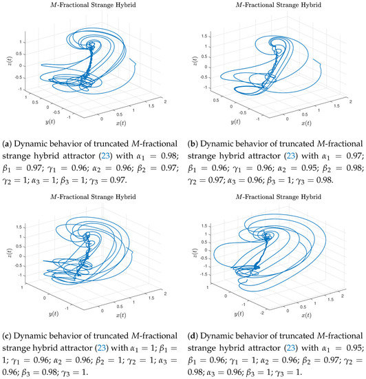
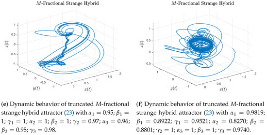Figure 13. Dynamic behaviors of the incommensurate truncated M-fractional strange hybrid attractor (23) for different orders with initial conditions $x\left(0\right)=2$, $y\left(0\right)=0$ and $z\left(0\right)=0$.

Case 2.

Choosing ${\alpha }_1=0.97$, ${\beta }_1=0.96$, ${\gamma }_1=0.96$ for the first state x; ${\alpha }_2=0.95$, ${\beta }_2=0.98$, ${\gamma }_2=0.97$ for the second state y; and ${\alpha }_3=0.96$, ${\beta }_3=1$, ${\gamma }_3=0.98$ for the third state z; Figure 13b shows interesting behavior for the truncated M-fractional strange hybrid attractor in Atangana–Baleanu sense.

Case 3.

Setting ${\alpha }_1=1$, ${\beta }_1=1$, ${\gamma }_1=0.96$ for the first state; ${\alpha }_2=0.96$, ${\beta }_2=1$, ${\gamma }_2=1$ for the second state; and ${\alpha }_3=0.96$, ${\beta }_3=0.98$, ${\gamma }_3=1$ for the last state; the truncated M-fractional strange hybrid attractor exhibits complex dynamics involving the Mittag–Leffler memory and the local M-derivative, see Figure 13c.

Case 4.

Considering for the state x the orders ${\alpha }_1=0.95$, ${\beta }_1=0.96$, ${\gamma }_1=1$; the values ${\alpha }_2=0.96$, ${\beta }_2=0.97$, ${\gamma }_2=0.98$ for the state y; and ${\alpha }_3=0.96$, ${\beta }_3=1$, ${\gamma }_3=1$ for z; Figure 13d depicts complex dynamics for the truncated M-fractional strange hybrid attractor in Atangana–Baleanu sense.

Case 5.

Next, to get the simulation shown in Figure 13e, in the state x was choosing ${\alpha }_1=0.95$, ${\beta }_1=1$, ${\gamma }_1=1$; for the state y${\alpha }_2=1$, ${\beta }_2=1$, ${\gamma }_2=0.97$; and the values ${\alpha }_3=0.96$, ${\beta }_3=0.95$, ${\gamma }_3=0.98$ in the state z.

Case 6.

The following parameters, randomly chosen, were set on the system (23): ${\alpha }_1=0.9819$, ${\beta }_1=0.8922$ and ${\gamma }_1=0.9521$ for the first state; ${\alpha }_2=0.8270$, ${\beta }_2=0.8801$ and ${\gamma }_2=1$ for the second; and ${\alpha }_3=1$, ${\beta }_3=1$, ${\gamma }_3=0.9740$ for the third state. Here, the inner scroll still remains because the external dynamics depict an attractor strange-like with quasi-periodic orbits. It can be see in Figure 13f.

The simulations shown in Figure 13, were developed by setting the initial conditions $x\left(0\right)=2$, $y\left(0\right)=0$ and $z\left(0\right)=0$; a step size of $\Delta t=1\times {10}^{-2}$ and a simulation time of $t=150$ [s].

• Observation. When ${\alpha }_i$, ${\beta }_i$ and ${\gamma }_i\to 1$, the classical strange hybrid attractor is obtained.

Chaos Analysis

In this part, a 0–1 test was carried out for the incommensurate M-fractional Strange attractor. This system was setting with a combination of earlier attractor orders for the cases 1, 2 until 5. In addition, six random orders were chosen for the case 6.

Table 3 shows growth rates for each incommensurate system, whereas Figure 14 and Figure 15, depict contrasting behaviors of the variables p and q. According to growth rates, one can see the presence of chaos in whole system due to $K\approx 1$.

Table 3. Growth rates for incommensurate M-Rucklidge attractor.

Derivative	${\mathit{x}}_1$	${\mathit{x}}_2$	${\mathit{x}}_3$	Case
M–Atangana–Baleanu	0.9962	0.9933	0.9120	Case 1
M–Atangana–Baleanu	0.9922	0.9942	0.9659	Case 2
M–Atangana–Baleanu	0.9897	0.9905	0.8573	Case 3
M–Atangana–Baleanu	0.9930	0.9773	0.9312	Case 4
M–Atangana–Baleanu	0.9946	0.9853	0.9442	Case 5
M–Atangana–Baleanu	0.9970	0.9901	0.9912	Case 6

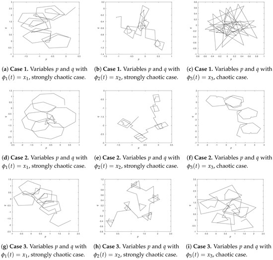
Figure 14. Variables p and q in the strange attractor (23) for different orders. (a–c) Case 1 with ${\alpha }_1=0.98$, ${\beta }_1=0.97$, ${\gamma }_1=0.96$, ${\alpha }_2=0.96$, ${\beta }_2=0.97$, ${\gamma }_2=1$, ${\alpha }_3=1$, ${\beta }_3=1$, ${\gamma }_3=0.97$; (d–f) Case 2 with ${\alpha }_1=0.97$, ${\beta }_1=0.96$, ${\gamma }_1=0.96$, ${\alpha }_2=0.95$, ${\beta }_2=0.98$, ${\gamma }_2=0.97$, ${\alpha }_3=0.96$, ${\beta }_3=1$, ${\gamma }_3=0.98$; (g–i) Case 3 with ${\alpha }_1=1$, ${\beta }_1=1$, ${\gamma }_1=0.96$, ${\alpha }_2=1$, ${\beta }_2=1$, ${\gamma }_2=1$, ${\alpha }_3=0.96$, ${\beta }_3=0.98$, ${\gamma }_3=1$, respectively.

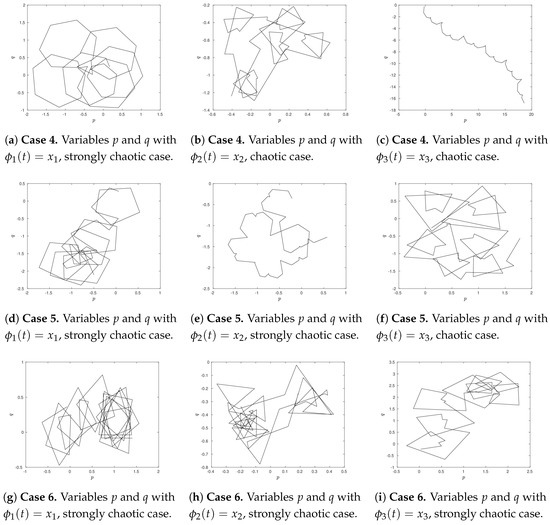
Figure 15. Variables p and q in Strange attractor (23) ffor different orders. (a–c) Case 4 with ${\alpha }_1=0.95$, ${\beta }_1=0.96$, ${\gamma }_1=1$, ${\alpha }_2=0.96$, ${\beta }_2=0.97$, ${\gamma }_2=0.98$, ${\alpha }_3=0.96$, ${\beta }_3=1$, ${\gamma }_3=1$; (d–f) Case 5 with ${\alpha }_1=0.95$, ${\beta }_1=1$, ${\gamma }_1=1$, ${\alpha }_2=1$, ${\beta }_2=0.97$, ${\gamma }_2=0.96$, ${\alpha }_3=0.96$, ${\beta }_3=0.95$, ${\gamma }_3=0.98$; (g–i) Case 6 with ${\alpha }_1=0.9819$, ${\beta }_1=0.8922$, ${\gamma }_1=0.9521$, ${\alpha }_2=0.8270$, ${\beta }_2=0.8801$, ${\gamma }_2=1$, ${\alpha }_3=1$, ${\beta }_3=1$, ${\gamma }_3=0.9740$, respectively.

On the other hand, sensitive dependence on initial conditions is one of the main components of chaos theory [22]. To carry out this analysis, we use the direct method [23]. This test consists of simulating a chaotic attractor with the same parameters, orders and trajectories very close to each other obtaining the difference between those trajectories. If the differences separate exponentially then the system is sensitive to initial conditions, in consequence, the system is chaotic.

In order to show the difficulty to predict behaviors in M-fractional Strange attractor, we perform a sensitivity test to initial conditions through the direct method. To do this, we set the numerical simulations as follows: the first trajectory with: $x_1=2,y_1=0,z_1=0$ and the second: $x_2=1.9,y_2=-0.1,z_2=-0.1$ for the Cases 1, 2, 3 until 6.

Figure 16, Figure 17 and Figure 18 show the difference between the above mentioned trajectories for the states $x,y$ and z, respectively. According to these numerical results, one can conclude that the three non-integer orders involving the novel M-derivative difficult the prediction of behaviors.

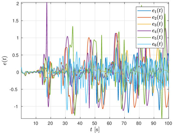
Figure 16. Differences between nearby starting trajectories for the state x in the incommensurate M-fractional Strange attractor.

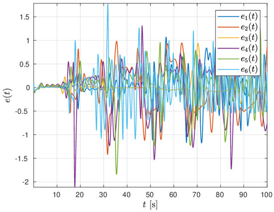
Figure 17. Differences between nearby starting trajectories for the state y in the incommensurate M-fractional strange attractor.

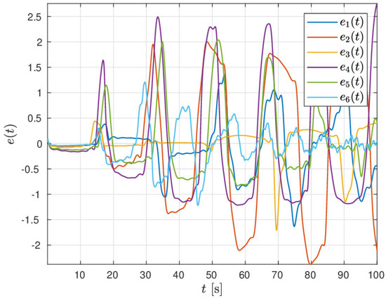
Figure 18. Differences between nearby starting trajectories for the state z in the incommensurate M-fractional strange attractor.

5. Conclusions

In this work, truncated M-fractional derivatives with three orders were suggested by using the truncated M-derivative and fractional operators with power-law, exponential decay and Mittag–Leffler kernel. These derivatives recover behaviors such as: Khalil conformable derivative, the M-derivative, alternative fractional derivative, generalized alternative fractional derivative, fractional derivatives of Liouville–Caputo, Caputo–Fabrizio and Atangana–Baleanu type or a combination of them with varying the orders $\alpha$, $\beta$ and $\gamma$, two for the truncated M-derivative and one of the fractional term related to power-law, exponential decay kernel or Mittag–Leffler function. These operators can describe memory, non-locality, elasticity and fractal effects at the same time.

Numerical results for three different attractors have been displayed to show the generalization of the proposed derivatives. The first attractor is concerned with the Rucklidge attractor with a power law, exponential decay law and Mittag–Leffler kernel. The second one considered the Shimizu–Morioka attractor with Mittag–Leffler memory and the last one example considered the incommensurate fractional hybrid strange attractor with orders ${\alpha }_i$, ${\beta }_i$ and ${\gamma }_i$ involving the generalized Mittag–Leffler function. For each derivative, we provided numerical schemes easy to carry out based on Lagrange interpolation. The numerical simulations showed complex dynamics and new attractor which proves that these new truncated M-ractional derivatives with memory can capture more complexities than other fractional operators, local or non-local. In the results obtained, one can see that all behaviors of the particular derivatives (conformable derivative of Khalil type, M-derivative, alternative fractional derivative, generalized alternative fractional derivative, or fractional derivatives of the Liouville–Caputo, Caputo–Fabrizio and Atangana–Baleanu type) are recovered.

Additionally, 0-1 test and sensitive dependence on initial conditions were considered to verify the existence of chaos in the above mentioned chaotic attractor. These tests, as well as the numerical simulations, were carried out by using MATLAB R2017a on a computer with the following features: AMD A12-9720P processor @2.7GHz, 8GB RAM under GNU Arch Linux with KDE Plasma 5.18.3.

We believe that these novels truncated M-fractional derivatives with three orders and power, exponential and strong Mittag–Leffler memories can be applied to various kinds of real-world problems and applications in many fields.

References

- Podlubny, I. Fractional Differential Equations: An Introduction to Fractional Derivatives, Fractional Differential Equations, to Methods of Their Solution and Some of Their Applications; Elsevier: Amsterdam, The Netherlands, 1998; Volume 198. [Google Scholar]
- Atangana, A.; Baleanu, D. New fractional derivatives with nonlocal and non-singular kernel: Theory and application to heat transfer model. arXiv 2016, arXiv:1602.03408. [Google Scholar] [CrossRef]
- Khalil, R.; Al Horani, M.; Yousef, A.; Sababheh, M. A new definition of fractional derivative. J. Comput. Appl. Math. 2014, 264, 65–70. [Google Scholar] [CrossRef]
- Katugampola, U.N. A new fractional derivative with classical properties. arXiv 2014, arXiv:1410.6535. [Google Scholar]
- Katugampola, U.N. New fractional integral unifying six existing fractional integrals. arXiv 2016, arXiv:1612.08596. [Google Scholar]
- Atangana, A.; Baleanu, D.; Alsaedi, A. New properties of conformable derivative. Open Math. 2015, 13. [Google Scholar] [CrossRef]
- Atangana, A.; Baleanu, D.; Alsaedi, A. Analysis of time-fractional Hunter-Saxton equation: A model of neumatic liquid crystal. Open Phys. 2016, 14, 145–149. [Google Scholar] [CrossRef]
- Sousa, J.; de Oliveira, E.C. On the local M-derivative. arXiv 2017, arXiv:1704.08186. [Google Scholar]
- Sousa, J.; de Oliveira, E.C. A new truncated M-fractional derivative type unifying some fractional derivative types with classical properties. arXiv 2017, arXiv:1704.08187. [Google Scholar]
- Baleanu, D.; Fernandez, A.; Akgül, A. On a Fractional Operator Combining Proportional and Classical Differintegrals. Mathematics 2020, 8, 360. [Google Scholar] [CrossRef]
- Anderson, D.R.; Ulness, D.J. Newly defined conformable derivatives. Adv. Dyn. Syst. Appl. 2015, 10, 109–137. [Google Scholar]
- Baleanu, D.; Fernandez, A. On fractional operators and their classifications. Mathematics 2019, 7, 830. [Google Scholar] [CrossRef]
- Caputo, M.; Fabrizio, M. A new definition of fractional derivative without singular kernel. Progr. Fract. Differ. Appl. 2015, 1, 1–13. [Google Scholar]
- Losada, J.; Nieto, J.J. Properties of a new fractional derivative without singular kernel. Progr. Fract. Differ. Appl. 2015, 1, 87–92. [Google Scholar]
- Salahshour, S.; Ahmadian, A.; Abbasb, Y.S.; Baleanu, D. M-fractional derivative under interval uncertainty: Theory, properties and applications. Chaos Solitons Fractals 2018, 117, 84–93. [Google Scholar] [CrossRef]
- Rucklidge, A. Chaos in models of double convection. J. Fluid Mech. 1992, 237, 209–229. [Google Scholar] [CrossRef]
- Kocamaz, U.E.; Uyaroğlu, Y. Controlling Rucklidge chaotic system with a single controller using linear feedback and passive control methods. Nonlinear Dyn. 2014, 75, 63–72. [Google Scholar] [CrossRef]
- Shimizu, T.; Morioka, N. On the bifurcation of a symmetric limit cycle to an asymmetric one in a simple model. Phys. Lett. A 1980, 76, 201–204. [Google Scholar] [CrossRef]
- Sprott, J. A dynamical system with a strange attractor and invariant tori. Phys. Lett. A 2014, 378, 1361–1363. [Google Scholar] [CrossRef]
- Toufik, M.; Atangana, A. New numerical approximation of fractional derivative with non-local and non-singular kernel: Application to chaotic models. Eur. Phys. J. Plus 2017, 132, 444. [Google Scholar] [CrossRef]
- Gottwald, G.A.; Melbourne, I. The 0-1 test for chaos: A review. In Chaos Detection and Predictability; Springer: Berlin/Heidelberg, Germany, 2016; pp. 221–247. [Google Scholar]
- Bensaïda, A. Noisy chaos in intraday financial data: Evidence from the American index. Appl. Math. Comput. 2014, 226, 258–265. [Google Scholar] [CrossRef]
- Lea, D.J.; Allen, M.R.; Haine, T.W. Sensitivity analysis of the climate of a chaotic system. Tellus A Dyn. Meteorol. Oceanogr. 2000, 52, 523–532. [Google Scholar] [CrossRef]
© 2020 by the authors. Licensee MDPI, Basel, Switzerland. This article is an open access article distributed under the terms and conditions of the Creative Commons Attribution (CC BY) license (http://creativecommons.org/licenses/by/4.0/).