The Asymmetric Alpha-Power Skew-t Distribution

Abstract

In this paper, we propose a new asymmetric and heavy-tail model that generalizes both the skew-t and power-t models. Properties of the model are studied in detail. The score functions and the elements of the observed information matrix are given. The process to estimate the parameters in model is discussed by using the maximum likelihood approach. Also, the observed information matrix is shown to be non-singular at the whole parametric space. Two applications to real data sets are reported to demonstrate the usefulness of this new model.

1. Introduction

In recent years, there has been considerable interest in the statistical literature related to flexible families of distributions able of modeling data that present high degree of asymmetry, with kurtosis index greater or smaller than the captured by normal model. In this context, two proposals that have shown a promising behavior in this type of situations are the skew-normal (SN) distribution of Azzalini [1] and the power-normal (PN) distribution of Durrans [2]. The SN distribution has been widely studied by many authors, and its main drawback is that it presents singular Fisher information matrix, implying the inference is useless from the theory of large samples using the maximum likelihood (ML) approach. Although the PN model has a shorter asymmetry range than SN distribution, it presents non-singular information matrix and can easily be extended to censored scenarios, as it has a simple distribution function, see, for example, in Martínez-Flórez et al. [3].

The PN model is part of a wide family of distributions known as alpha-power, which has been widely studied by many authors. In addition to the normal distribution, the Birnbaum–Saunders (BS) distribution [4] has also been considered, see, for example, in Martínez-Flórez et al. [5], who propose an extension of the BS distribution based on the asymmetric alpha-power family of distributions to illustrate the applicability of the new proposal with a data set is related to the lifetimes in cycles $\times {10}^{-3}$$n=101$ aluminum $6061-T6$ pieces cut in parallel angle to the rotation direction of rolling at the rate of 18 cycles per second and maximum stress of 21.000 psi. More details of the PN distribution can be found in Gupta and Gupta [6] and Pewsey et al. [7].

An alternative propose for modeling asymmetric data that unifies the two previous approaches was introduced by Martínez-Flórez et al. [8]. The proposed model, which is called alpha-power skew-normal (APSN), has non-singular Fisher information matrix, and it can fit data with much more asymmetry than PN models it can handle. In addition, symmetry can be tested by using the likelihood ratio statistic, as the properties of large samples are satisfied for the ML estimator.

Another set of distributions with non-singular information matrices, useful for modeling asymmetric and heavy-tailed data, are based on generalizations of the Student-t distribution, see, for example, in [9,10,11,12,13]. Azzalini and Capitanio [9] for example, introduced a skew-t (ST) distribution as an extension of the SN model for modeling asymmetric and heavy-tailed data as follows; The random variable X is said to have the ST distribution with parameter $\lambda$ and degrees of freedom $\nu$, if X has the probability density function (PDF) given by

$$f_{ST}(x;\lambda ,\nu )=2f_T\left(x;\nu \right){\mathcal{F}}_T\left(\lambda \sqrt{\frac{\nu +1}{x^2+\nu }}x;\nu +1\right),x\in \mathbb{R}$$

(1)

where $\lambda \in \mathbb{R}$ is a parameter that controls the skewness of the distribution, and $f_T\left(·;\nu \right)$ and ${\mathcal{F}}_T\left(·;\nu \right)$ denote the PDF and the cumulative distribution function (CDF) of a standard Student-t distribution with $\nu$ degree of freedom, respectively. The ST distribution, like an extension of the SN model, inherits the problem of the singularity of the information matrix and before this inconvenience Zhao and Kim [14] proposed the power Student-t (PT) distribution, whose information matrix is non-singular and for a given degree of freedom, the kurtosis range surpasses the kurtosis range of the skew-t model at all times. The PT distribution is defined as follows. The random variable X is said to have the PT distribution with parameter $\alpha$, and degrees of freedom $\nu$, if X has PDF given by

$$f_{PT}(x;\alpha ,\nu )=\alpha f_T\left(x;\nu \right){\left[{\mathcal{F}}_T\left(x;\nu \right)\right]}^{\alpha -1},x\in \mathbb{R}$$

(2)

where $\alpha >0$ is a parameter that controls the form of the distribution, and, again, $f_T\left(·;\nu \right)$ and ${\mathcal{F}}_T\left(·;\nu \right)$ denote the PDF and the CDF of a standard Student-t distribution, respectively.

Based on the properties of the ST model, to fit data with high degree of asymmetry and the characteristic of the PN model to capture kurtosis larger than the normal model, in this paper, we introduce a new distribution for modeling asymmetric and heavy-tailed data. The proposed model possess non-singular information matrix, and it is able to fit data with far more asymmetry than ST and PT models can handle and with large sample properties satisfied for the ML estimator. The model introduced in this paper is named as alpha-power skew-t (APST) model and it extends both, ST and PT models. The APSN model by Martínez-Flórez et al. [8] is also a particular case when $\nu$ tends to infinite. Note that symmetry can be tested using the likelihood ratio statistics with its large sample chi-square distribution.

The rest of this paper is organized as follows. Section 2 introduces the APST model and some of its properties like moments are studied. In particular, skewness and kurtosis indices are computed showing that their ranges surpass those of the ST and PT models. Section 3 deals with the ML estimation for the location-scale situation and its observed information matrix is derived. The extension to censored data is also presented. Finally, two applications are shown in Section 4, revealing that the model proposed can present much improvement over competitors.

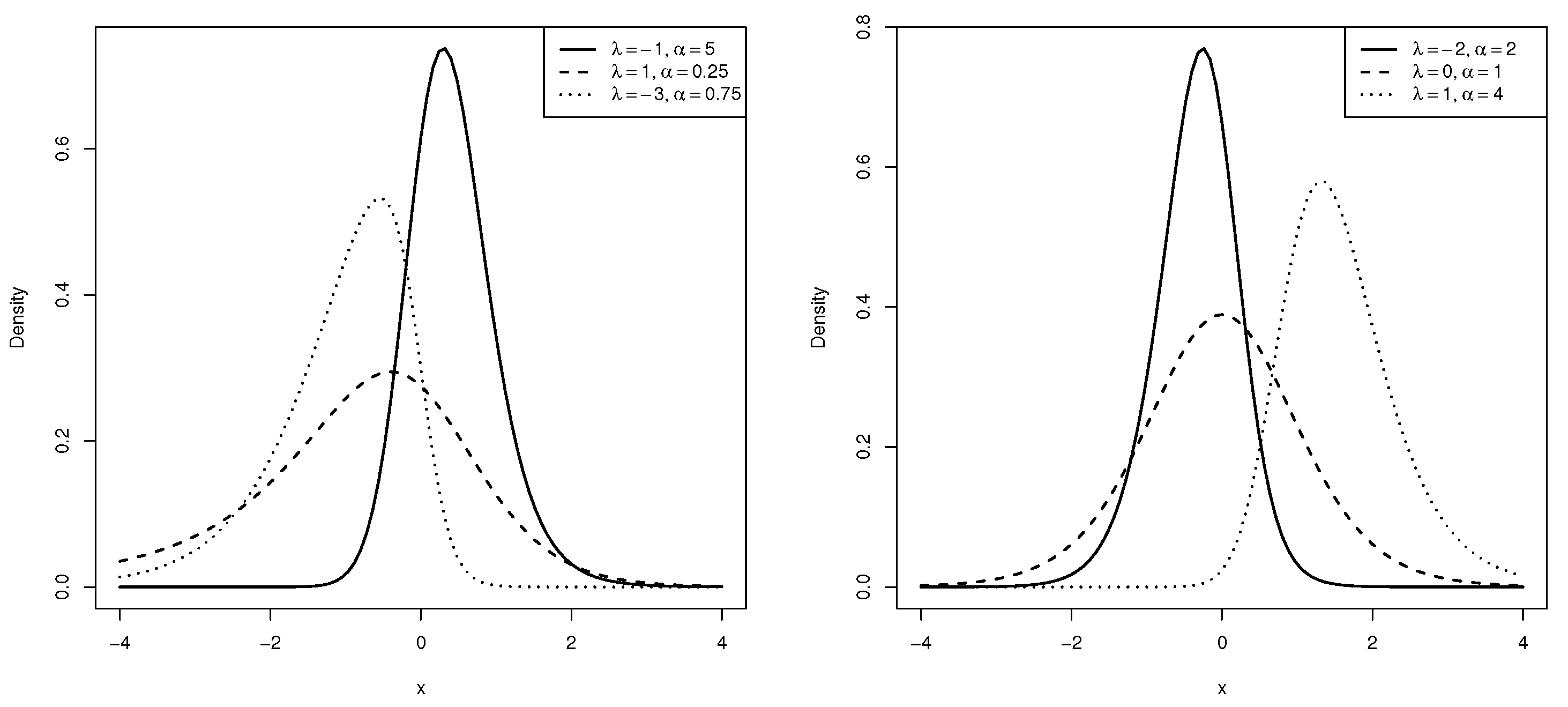
2. The Alpha-Power Skew-t Distribution

Definition 1.

The random variable X is said to have an alpha-power skew-t (APST) distribution, if X has PDF given by

$$f_{APST}(x;\lambda ,\alpha ,\nu )=\alpha f_{ST}(x;\lambda ,\nu ){\left[{\mathcal{F}}_{ST}(x;\lambda ,\nu )\right]}^{\alpha -1},$$

(3)

for $x\in \mathbb{R}$, $\lambda \in \mathbb{R}$, and $\alpha ,\nu \in {\mathbb{R}}^{+}$. Functions $f_{ST}(·)$ and ${\mathcal{F}}_{ST}(·)$ denote the PDF and the CDF of the standard ST distribution. A random variable having $f_{APST}(x;\lambda ,\alpha ,\nu )$ distribution is denoted shortly by $X\sim \mathrm{APST}(\lambda ,\alpha ,\nu )$.

Figure 1 displays the form of the APST distribution for some selected values of the parameters $\lambda$ and $\alpha$ for $\nu =6$. Note from the figure that the asymmetry and kurtosis of the APST distribution are affected by the parameters $\alpha$ and $\lambda$; therefore, the APST model is more flexible to model data that can be highly skewed, as well as heavier tails than ST and PT models.

Figure 1. Probability density function of $\mathrm{APST}(\lambda ,\alpha ,10)$ for some values of $\lambda$ and $\alpha$.

The following result provides some special cases of the model (3), which occur for different values of $\lambda$, $\alpha$, and $\nu$.

Proposition 1.

Let $X\sim \mathrm{APST}(\lambda ,\alpha ,\nu )$,

(i) 

if $\lambda =0$, then $X\sim \mathrm{PT}(\alpha ,\nu )$,

(ii) 

if $\alpha =1$, then $X\sim \mathrm{ST}(\lambda ,\nu )$,

(iii) 

if $\lambda =0$ and $\alpha =1$, then $X\sim \mathrm{T}(\nu )$, where $\mathrm{T}(\nu )$ denotes the Student-t disribution with ν degree of freedom.

(iv) 

if $\nu \to +\infty$, then $X\sim \mathrm{APSN}(\lambda ,\alpha )$,

(v) 

if $\lambda =0$ and $\nu \to +\infty$, then $X\sim \mathrm{PN}(\alpha )$,

(vi) 

if $\alpha =1$ and $\nu \to +\infty$, then $X\sim \mathrm{SN}(\lambda )$,

(vii) 

if $\lambda =0$, $\alpha =1$ and $\nu \to +\infty$, then $X\sim \mathrm{N}(0,1)$,

Proof. 

The proof of (i)–(vii) is immediate from the definition of APST distribution. □

2.1. Moments

The following proposition presents an expression to compute the k-th moment of a random variable $\mathrm{APST}(\lambda ,\alpha ,\nu )$.

Proposition 2.

Let $X\sim \mathrm{APST}(\lambda ,\alpha ,\nu )$, then

$$\mathbb{E}\left[X^k\right]=\mathbb{E}\left[{\left({\mathcal{F}}_{ST}^{-1}(Y;\lambda ,\nu )\right)}^k\right]$$

(4)

where Y follows a $\mathrm{Beta}(\alpha ,1)$ distribution and ${\mathcal{F}}_{ST}^{-1}(·;\lambda ,\nu )$ is the inverse of the function ${\mathcal{F}}_{ST}(·;\lambda ,\nu )$.

Proof. 

We have by definition that

$$\mathbb{E}\left[X^k\right]={\int }_{\mathbb{R}}{x}^k\alpha f_{ST}(x){\left({\mathcal{F}}_{ST}(x;\lambda ,\nu )\right)}^{\alpha -1}dx$$

thus, letting $y={\mathcal{F}}_{ST}(x;\lambda ,\nu )$, then $x={\mathcal{F}}_{ST}^{-1}(y;\lambda ,\nu )$, it follows that

$$\mathbb{E}\left[X^k\right]={\int }_0^1\alpha {\left({\mathcal{F}}_{ST}^{-1}(y;\lambda ,\nu )\right)}^k{y}^{\alpha -1}dy$$

which is the expected value of the function ${\left({\mathcal{F}}_{ST}^{-1}(Y;\lambda ,\nu )\right)}^k$, where Y follows a beta distribution with parameters $\alpha$ and 1. □

The indices of skewness $(\sqrt{{\beta }_1})$ and kurtosis $({\beta }_2)$ of APST distribution can be calculated by using the moments (4) as follows,

$$\sqrt{{\beta }_1}=\frac{{\mu }_3-3{\mu }_1{\mu }_2+2{\mu }_1^3}{{({\mu }_2-{\mu }_1^2)}^{3/2}}\mathrm{and}{\beta }_2=\frac{{\mu }_4-4{\mu }_1{\mu }_3+6{\mu }_2{\mu }_1^2-3{\mu }_1^4}{{({\mu }_2-{\mu }_1^2)}^2}$$

where ${\mu }_k=\mathbb{E}[X^k]$ for $k=1,\cdots ,4$. Table 1 presents the ranges of possible values for the indices of asymmetry and kurtosis for $\mathrm{ST}(\lambda ,\nu )$, $\mathrm{PT}(\alpha ,\nu )$, and $\mathrm{APST}(\lambda ,\alpha ,\nu )$ distributions, for values of $\lambda$ between −40 and 40, values of $\alpha$ between 0.5 and 50, and for values of $\nu =2,3,4,5,6,7$. It can seen from Table 1 that the length of the admissible intervals for the skewness and the kurtosis parameters of the APST distribution are larger than the corresponding intervals of the ST and PT distributions. This is an indicator that the APST model is more flexible in terms of asymmetry and kurtosis than the ST and PT models.

Table 1. Skewness and kurtosis for the models $\mathrm{ST}(\lambda ,\nu )$, $\mathrm{PT}(\alpha ,\nu )$, and $\mathrm{APST}(\lambda ,\alpha ,\nu )$, for $\lambda \in (-40,40)$, $\alpha \in (0.5,50)$ and $\nu =2,\cdots 7$.

	Skew$—\mathit{t}$		Power$—\mathit{t}$		Alpha—Power Skew $—\mathit{t}$
$\mathbf{\nu }$	Skewness	Kurtosis	Skewness	Kurtosis	Skewness	Kurtosis
2	$(-0.963,0.963)$	$(3.170,3.489)$	$(-0.119,3.040)$	$(1.552,10.436)$	$(-2.452,14.314)$	$(1.395,864.385)$
3	$(-0.950,0.950)$	$(3.146,3.357)$	$(-0.086,1.362)$	$(1.325,3.223)$	$(-2.130,4.902)$	$(1.628,114.098)$
4	$(-1.853,1.853)$	$(5.099,7.824)$	$(-0.530,1.178)$	$(3.461,5.299)$	$(-1.898,3.215)$	$(3.153,29.874)$
5	$(-0.947,0.947)$	$(3.051,3.327)$	$(-0.475,0.271)$	$(1.176,3.130)$	$(-1.968,3.046)$	$(3.862,19.925)$
6	$(-1.681,1.681)$	$(4.554,7.279)$	$(-0.533,1.118)$	$(3.974,5.173)$	$(-1.681,2.145)$	$(3.892,11.893)$
7	$(-0.944,0.944)$	$(3.007,3.367)$	$(-0.710,0.243)$	$(1.264,3.082)$	$(-1.535,2.536)$	$(3.136,15.924)$

2.2. Distribution Function

Proposition 3.

Let $X\sim \mathrm{APST}(\lambda ,\alpha ,\nu )$, then the CDF of X, namely, ${\mathcal{F}}_{APST}(x;\lambda ,\alpha ,\nu )$ is

$${\mathcal{F}}_{APST}(x;\lambda ,\alpha ,\nu )={\left[{\mathcal{F}}_{ST}(x;\lambda ,\nu )\right]}^{\alpha },x\in \mathbb{R}.$$

(5)

Proof. 

The proof is immediate and it follows from results of Durrans [2]. □

The inversion method can be used to generate a random variable with APST distribution. Thus, taking $\lambda \in \mathbb{R}$, $\alpha ,\nu \in {\mathbb{R}}^{+}$ and a random variable with uniform distribution, namely, $U\sim \mathrm{U}(0,1)$, random variable X with $\mathrm{APST}(\lambda ,\alpha ,\nu )$ distribution is generated by taking

$$X={\mathcal{F}}_{ST}^{-1}\left(U^{1/\alpha };\lambda ,\nu \right).$$

Remark 1.

We consider a truncated $\mathrm{APST}(\lambda ,\alpha )$ distribution to obtain a new and useful lifetime distribution. A random variable T has a truncated alpha-power skew-t distribution (at zero), denoted by $\mathit{TAPST}(\lambda ,\alpha ,\nu )$, if its PDF is given by

$$f(t)=\frac{\alpha f_{ST}(t,\lambda ,\nu ){\left[{\mathcal{F}}_{ST}(t,\lambda ,\nu )\right]}^{\alpha -1}}{1-{\left[{\mathcal{F}}_{ST}(0,\lambda ,\nu )\right]}^{\alpha }};t>0$$

(6)

The survival and hazard rate functions of a random variable T following a $\mathrm{TAPST}(\lambda ,\alpha ,\nu )$ distribution are given by

$${\mathcal{S}}_T(t)=P(T>t)=\frac{1-{\left[{\mathcal{F}}_{ST}(0,\lambda ,\nu )\right]}^{\alpha }-{\left[{\mathcal{F}}_{ST}(t,\lambda ,\nu )\right]}^{\alpha }}{1-{\left[{\mathcal{F}}_{ST}(0,\lambda ,\nu )\right]}^{\alpha }};t>0$$

(7)

and

$$h_T(t)=\frac{\alpha f_{ST}(t,\lambda ,\nu ){\left[f_{ST}(t,\lambda ,\nu )\right]}^{\alpha -1}}{1-{\left[{\mathcal{F}}_{ST}(0,\lambda ,\nu )\right]}^{\alpha }-{\left[{\mathcal{F}}_{ST}(t,\lambda ,\nu )\right]}^{\alpha }};t>0$$

(8)

respectively.

2.3. Location and Scale Extension

We can also consider a generalization of a APST distribution by adding location and scale parameters. The following definition gives a generalization of the APST model.

Definition 2.

Let $X\sim \mathrm{APST}(\lambda ,\alpha ,\nu )$. The APST density of location and scale is defined as the distribution of $Y=\mu +\sigma X$, for $\mu \in \mathbb{R}$ and $\sigma >0$. The corresponding PDF is given by

$$f_{APST}(y;\mu ,\sigma ,\lambda ,\alpha ,\nu )=\frac{\alpha }{\sigma }{f}_{ST}\left(\frac{y-\mu }{\sigma };\lambda ,\nu \right){\left[{\mathcal{F}}_{ST}\left(\frac{y-\mu }{\sigma };\lambda ,\nu \right)\right]}^{\alpha -1},x\in \mathbb{R},$$

(9)

for $\lambda \in \mathbb{R}$ and $\alpha ,\nu \in {\mathbb{R}}^{+}$. A random variable following a APST distribution of location and scale is denoted by $Y\sim \mathrm{APST}(\mu ,\sigma ,\lambda ,\alpha ,\nu )$.

The k-th moment of a random variable $Y\sim \mathrm{APST}(\mu ,\sigma ,\lambda ,\alpha ,\nu )$ can be obtained from the formula

$$\mathbb{E}\left[Y^k\right]=\sum _{i=0}^k\left(\genfrac{}{}{0pt}{}{k}{i}\right){\mu }^i{\sigma }^{k-i}\mathbb{E}\left[X^{k-i}\right],$$

where $X\sim \mathrm{APST}(\lambda ,\alpha ,\nu )$.

3. Statistical Inference for APST Distribution

This section concerns likelihood inference about the parameter vector $\mathit{\theta }={(\mu ,\sigma ,\lambda ,\alpha ,\nu )}^{\top }$ of the location-scale family defined in Equation (9). Let $\mathbf{Y}={(Y_1,\cdots ,Y_n)}^{\top }$ be a random sample of the distribution $\mathrm{APST}(\mu ,\sigma ,\lambda ,\alpha ,\nu )$. The log-likelihood function for $\mathit{\theta }={(\mu ,\sigma ,\lambda ,\alpha ,\nu )}^{\top }$ can be written as follows,

$$\begin{array}{ll}\ell (\mathit{\theta };\mathbf{Y})\propto n& log\alpha -nlog\sigma -\frac{n}{2}log\nu \hfill \\ & +nlog\Gamma \left(\frac{\nu +1}{2}\right)-nlog\Gamma \left(\frac{\nu }{2}\right)-\frac{\nu +1}{2}\sum _{i=1}^{n}log\left(1+\frac{z_i^2}{\nu }\right)\hfill \\ & +\sum _{i=1}^{n}log{\mathcal{F}}_T\left(\lambda z_i\sqrt{\frac{\nu +1}{z_i^2+\nu }};\nu +1\right)+(\alpha -1)\sum _{i=1}^{n}log{\mathcal{F}}_{ST}\left(z_i;\lambda ,\nu \right)\hfill \end{array}$$

(10)

where $z_i=(y_i-\mu )/\sigma$. Thus, by differentiating the log-likelihood function, we obtain the following score equations,

$$\begin{array}{cc}\hfill \frac{\partial \ell (\mathit{\theta };\mathbf{Y})}{\partial \mu }& =\frac{\nu +1}{\sigma \nu }\sum _{i=1}^n{z}_i{\left(1+\frac{z_i^2}{\nu }\right)}^{-1}\hfill \\ \hfill & -\frac{\lambda }{\sigma }\sum _{i=1}^n{w}_i{\left(1+\frac{z_i^2}{\nu }\right)}^{-1}\frac{f_T\left(\lambda z_i{w}_i;\nu +1\right)}{{\mathcal{F}}_T\left(\lambda z_i{w}_i;\nu +1\right)}-\frac{\alpha -1}{\sigma }\sum _{i=1}^n\frac{f_{ST}(z_i;\lambda ,\nu )}{{\mathcal{F}}_{ST}(z_i;\lambda ,\nu )}=0\hfill \end{array}$$

(11)

$$\begin{array}{cc}\hfill \frac{\partial \ell (\mathit{\theta };\mathbf{Y})}{\partial \sigma }& =-\frac{n}{\sigma }+\frac{\nu +1}{\sigma \nu }\sum _{i=1}^n{z}_i^2{\left(1+\frac{z_i^2}{\nu }\right)}^{-1}-\frac{\lambda }{\sigma }\sum _{i=1}^n{z}_i{w}_i{\left(1+\frac{z_i^2}{\nu }\right)}^{-1}\frac{f_T\left(\lambda z_i{w}_i;\nu +1\right)}{{\mathcal{F}}_T\left(\lambda z_i{w}_i;\nu +1\right)}\hfill \\ \hfill & -\frac{\alpha -1}{\sigma }\sum _{i=1}^n{z}_i\frac{f_{ST}(z_i;\lambda ,\nu )}{{\mathcal{F}}_{ST}(z_i;\lambda ,\nu )}=0\hfill \end{array}$$

(12)

$$\begin{array}{ll}\frac{\partial \ell (\mathit{\theta };\mathbf{Y})}{\partial \lambda }& =\sum _{i=1}^n{z}_i{w}_i\frac{f_T\left(\lambda z_i{w}_i;\nu +1\right)}{{\mathcal{F}}_T\left(\lambda z_i{w}_i;\nu +1\right)}-\frac{\alpha -1}{\pi (1+{\lambda }^2)}\sum _{i=1}^n\frac{{\left(1+(1+{\lambda }^2)z_i^2/\nu \right)}^{-\frac{\nu }{2}}}{{\mathcal{F}}_{ST}(z_i;\lambda ,\nu )}=0,\hfill \end{array}$$

(13)

$$\begin{array}{ll}\frac{\partial \ell (\mathit{\theta };\mathbf{Y})}{\partial \alpha }& =\frac{n}{\alpha }+\sum _{i=1}^{n}log{\mathcal{F}}_{ST}(z_i;\lambda ,\nu )=0,\hfill \end{array}$$

(14)

$$\begin{array}{ll}\frac{\partial \ell (\mathit{\theta };\mathbf{Y})}{\partial \nu }& =\frac{n\alpha }{2}\left(\psi \left(\frac{\nu +1}{2}\right)-\psi \left(\frac{\nu }{2}\right)-\frac{1}{\nu }\right)-\frac{1}{2}\sum _{i=1}^{n}log\left(1+\frac{z_i^2}{\nu }\right)\hfill \\ & +\frac{\nu +1}{2{\nu }^2}\sum _{i=1}^n{z}_i^2{\left(1+\frac{z_i^2}{\nu }\right)}^{-1}\hfill \\ & +\frac{\lambda }{2\nu (\nu +1)}\sum _{i=1}^n{z}_i^3{w}_i{\left(1+\frac{z_i^2}{\nu }\right)}^{-1}\frac{f_T\left(\lambda z_i{w}_i;\nu +1\right)}{{\mathcal{F}}_T\left(\lambda z_i{w}_i;\nu +1\right)}\hfill \\ & -\frac{\lambda }{2\nu (\nu +1)}\sum _{i=1}^n{z}_i{w}_i{\left(1+\frac{z_i^2}{\nu }\right)}^{-1}\frac{f_T\left(\lambda z_i{w}_i;\nu +1\right)}{{\mathcal{F}}_T\left(\lambda z_i{w}_i;\nu +1\right)}\hfill \\ & -\frac{(\alpha -1)}{2\pi (\nu +1)}\frac{\lambda }{(1+{\lambda }^2)}\sum _{i=1}^n\frac{{\left(1+(1+{\lambda }^2)z_i^2/\nu \right)}^{-\frac{\nu }{2}}}{{\mathcal{F}}_{ST}(z_i;\lambda ,\nu )}+\frac{\alpha -1}{2}\sum _{i=1}^n\frac{g(z_i;\nu )}{{\mathcal{F}}_{ST}\left(z_i;\lambda ,\nu \right)}=0\hfill \end{array}$$

(15)

where $\psi (·)$ is the digamma function, $w_i=\sqrt{\frac{\nu +1}{x_i^2+\nu }}$ for $i=1,\cdots ,n$, and $g(x;\nu )$ is the function defined by

$$\begin{array}{cc}\hfill g(x;\nu )& ={\int }_{-\infty }^x\left\{\frac{(\nu +1)}{{\nu }^2}{s}^2{\left(1+\frac{s^2}{\nu }\right)}^{-1}-log\left(1+\frac{s^2}{\nu }\right)\right\}{f}_{ST}(s;\lambda ,\nu )ds\hfill \\ \hfill & -\frac{\lambda }{\pi \nu }{\int }_{-\infty }^{x}s{\left(1+\frac{s^2}{\nu }\right)}^{-1}{\left\{1+(1+{\lambda }^2)\frac{s^2}{\nu }\right\}}^{-\frac{\nu +2}{2}}ds\hfill \end{array}$$

(16)

Equations (11)–(15) include nonlinear functions; therefore, it is not possible to obtain explicit forms of the maximum likelihood estimators (MLEs), and they must be calculated by using numerical methods. In this work, we used the maxLik function of R Development Core Team [15] which uses the Newton–Raphson optimization method. The elements of the observed information matrix are easily obtained after calculating the second derivative of the log-likelihood function and multiplying by −1, that is,

$$j_{{\mathit{\theta }}_i{\mathit{\theta }}_k}=-\frac{\partial \ell (\mathit{\theta };\mathbf{Y})}{\partial {\mathit{\theta }}_i\partial {\mathit{\theta }}_k},i,k=1,2,\cdots ,5$$

(17)

where $\mathit{\theta }={(\mu ,\sigma ,\lambda ,\alpha ,\nu )}^{\top }$. This elements are given in the Appendix A. To find the standard errors (EE) of the MLEs and calculate confidence intervals, the information matrix $\mathbf{I}$ (or Fisher information) must be calculated, which is defined as the expected value of the second derived from the log-likelihood function or less the expected value of the Hessian matrix; from this matrix, we calculate the EE as the diagonal elements of the inverse of this matrix. The elements of the $\mathbf{I}$ matrix are obtained as

$$\mathbf{I}(i,k)=-E\left(\frac{\partial \ell (\mathit{\theta };\mathbf{Y})}{\partial {\theta }_i\partial {\theta }_k}\right),i,k=1,2,\cdots ,5$$

(18)

The role of the Fisher information in the asymptotic theory of maximum-likelihood estimation was emphasized by Ronald Fisher following some initial results by Francis Edgeworth, see Lehman and Casella [16] and Frieden [17] for more details. The Fisher-information matrix is used to calculate the covariance matrices associated with maximum-likelihood estimates, and it can also be used in the formulation of test statistics, such as the Wald test.

As the expected value under the APST distribution and the second-order derivatives are not direct, numerical methods must be used to obtain the explicit form of the information matrix I. Therefore, we use the observed information matrix to calculate the standard errors in the rest of the document.

When $\nu$ tends to infinite the ST distribution converges to the SN distribution and we recall that the information matrix of a random variable $X\sim \mathrm{SN}(\mu ,\sigma ,\lambda )$ which is denoted by ${\mathbf{I}}_{\lambda }(\mathit{\phi })$, where $\mathit{\phi }={(\mu ,\sigma ,\lambda )}^{\top }$, is singular for $\lambda =0$. Therefore, it is convenient to use a centered parameterization of the ST distribution proposed by Arellano-Valle and Azzalini [18].

The centered parameterization of the SN distribution was proposed as an alternative to the problem of singularity of the information matrix of the SN when $\lambda =0$. Arellano-Valle and Azzalini [19] proposed a second representation of the SN by defining a new random variable X as

$$X=\mu +\sigma \left(\frac{Z-\mathbb{E}[Z]}{\sqrt{\mathrm{Var}[Z]}}\right),$$

where $\mu \in \mathbb{R}$ and $\sigma >0$ are parameters of the random variable X and $Z\sim \mathrm{SN}(\lambda )$. This representation is called centered parameterization, as $\mathbb{E}[X]=\mu$ and $\mathrm{Var}[X]={\sigma }^2$ and it is denoted by $\mathrm{CSN}(\mu ,\sigma ,{\gamma }_1)$, where $-0.9953<{\gamma }_1<0.9953$. Under the centered parameterization model, $\mu$, $\sigma$, and ${\gamma }_1=\sqrt{{\beta }_1}$ represent the mean, the standard deviation and the skewness index of X, respectively. If $Z\sim \mathrm{SN}(\lambda )$ then $\mathbb{E}[Z]=b\delta$ and $\mathrm{Var}[Z]=1-{(b\delta )}^2$, where $b=\sqrt{2/\pi }$ and $\delta =\lambda /\sqrt{1+{\lambda }^2}$; it has that the random variable X can be written as $X=\mu +\sigma Z$ which has $\mathrm{SN}({\lambda }_1,{\lambda }_2,\lambda )$ distribution, where

$${\lambda }_1=\mu -c\sigma {\gamma }_1^{1/3},{\lambda }_2=\sigma \sqrt{1+c^2{\gamma }_1^{2/3}},\lambda =\frac{c{\gamma }_1^{1/3}}{\sqrt{b^2+c^2(b^2-1){\gamma }_1^{2/3}}}$$

(19)

with $c={\{2/(4-\pi )\}}^{1/3}$. Under this denomination, the information matrix can be written as ${\mathbf{I}}_{{\gamma }_1}={\mathbf{D}}^{\top }{\mathbf{I}}_{\lambda }\mathbf{D}$, where $\mathbf{D}$ is a matrix that represents the derivative of the parameters of the standard representation (${\lambda }_1$, ${\lambda }_2$ and $\lambda$) regarding to the new parameters ($\mu$, $\sigma$ and ${\gamma }_1$). It also follows that the information matrix converges to a diagonal matrix ${\Sigma }_c^{-1}=\mathrm{diag}({\sigma }^2,{\sigma }^2/2,6)$ when $\lambda \to 0$. This guarantees the existence and uniqueness of the MLEs of ${\lambda }_1$ and ${\lambda }_2$ for each fixed value of $\lambda$.

Following this same line of thought, we suppose that Y follows the model (1) with location parameter $\mu \in \mathbb{R}$ and scale parameter $\sigma >0$, that is,

$$f_{ST}(y;\mu ,\sigma ,\lambda ,\nu )=\frac{2}{\sigma }{f}_T\left(\frac{y-\mu }{\sigma };\nu \right){\mathcal{F}}_T\left(\lambda \sqrt{\frac{\nu +1}{Q_y+\nu }}\left(\frac{y-\mu }{\sigma }\right);\nu +1\right),y\in \mathbb{R}$$

(20)

where $\lambda \in \mathbb{R}$ and $Q_y={((y-\mu )/\sigma )}^2$. This representation relates to the direct parameterization of the ST distribution with parameter vector $\rho ={(\mu ,\sigma ,\lambda ,\nu )}^{\top }$. It follows that $Z_T=(Y-\mu )/\sigma \sim \mathrm{ST}(\lambda ,\nu )$, and by the stochastic representation of the ST distribution is given by $Z_T=Z/\sqrt{V}$, where $Z\sim \mathrm{SN}(\lambda )$ and $V\sim {\chi }_{\nu }^2/\nu$. This entails to compute the first four cumulants of $Z_T$ denoted by ${\mu }_1(\delta ,\nu )$, ${\mu }_2(\delta ,\nu )$, ${\mu }_3(\delta ,\nu )$ and ${\mu }_4(\delta ,\nu )$, see [18]. The centered parameterization of the ST distribution of a random variable Y comes by defining

$$\begin{array}{cc}\hfill {\mu }_t& =\mathbb{E}[Y]=\mu +\sigma {\mu }_1(\delta ,\nu )=\mu +\sigma b_{\nu }\delta \hfill \\ \hfill {\sigma }_t^2& =\mathrm{Var}[Y]={\sigma }^2{\mu }_2(\delta ,\nu )={\eta }^2\left\{\frac{\nu }{\nu -2}-b_{\nu }^2{\delta }^2\right\},\hfill \end{array}$$

$$\begin{array}{cc}\hfill {\gamma }_{1t}& =\frac{{\mu }_3(\delta ,\nu )}{{\mu }_2{(\delta ,\nu )}^{3/2}}=\frac{b_{\nu }\delta }{{\mu }_2{(\delta ,\nu )}^{3/2}}\left\{\frac{\nu (3-{\delta }^2)}{\nu -3}-\frac{3\nu }{\nu -2}+2b_{\nu }^2{\delta }^2\right\}\hfill \\ \hfill {\gamma }_{2t}& =\frac{{\mu }_4(\delta ,\nu )}{{\mu }_2{(\delta ,\nu )}^2}=\frac{1}{{\mu }_2{(\delta ,\nu )}^2}\left\{\frac{3{\nu }^2}{(\nu -2)(\nu -4)}-\frac{4b_{\nu }^2{\delta }^2\nu (3-{\delta }^2)+\frac{6b_{\nu }^2{\delta }^2\nu }{\nu -2}-4b_{\nu }^4{\delta }^4}{\nu -3}\right\}-3.\hfill \end{array}$$

The new representation is defined as the centered skew-t distribution with parameter vector $\tilde{\rho }={(\mu ,{\sigma }^2,{\gamma }_1,{\gamma }_2)}^{\top }$. According to Arellano-Valle and Azzalini [18], the information matrix of this representation can be written as

$$\mathbf{I}(\tilde{\rho })={\mathbf{B}}^{\top }\mathbf{I}(\rho )\mathbf{B},$$

where $\mathbf{B}$ is a matrix representing the derivative of the parameter vector $\rho$ with respect to the new vector $\tilde{\rho }$. It can shown that $b_{\nu }\to b$ when $\nu \to \infty$, see [18]. Therefore, the parameters of the centered ST model converge to ${\mu }_t\to \mu$, ${\sigma }_t^2\to {\sigma }^2$, and ${\gamma }_{1t}\to {\gamma }_1$ when $\nu \to \infty$, that is, the parameters of the CSN. As $Z_T\to \mathrm{SN}(\lambda )$ when $\nu \to \infty$, it follows that the random variable Y converges to a distribution with information matrix

$$\mathbf{I}(\mu ,{\sigma }^2,{\gamma }_1,\alpha )=\left(\begin{array}{cc}{\mathbf{I}}_{{\mathit{\theta }}_1{\mathit{\theta }}_1}& {\mathbf{I}}_{{\mathit{\theta }}_1,\alpha }\\ {\mathbf{I}}_{{\mathit{\theta }}_1,\alpha }^{\top }& I_{\alpha ,\alpha }\end{array}\right),$$

(21)

where the elements of the diagonal correspond to the information of the parameter vector ${\mathit{\theta }}_1=(\mu ,{\sigma }^2,{\gamma }_1)$ and $\alpha$, and ${\mathbf{I}}_{{\mathit{\theta }}_1,\alpha }$ is the joint information of ${\mathit{\theta }}_1={(\mu ,{\sigma }^2,{\gamma }_1)}^{\top }$ and $\alpha$. Now, when $\lambda \to 0$ and $\alpha =1$, it can be shown that ${\mathbf{I}}_{{\mathit{\theta }}_1{\mathit{\theta }}_1}\to \mathrm{diag}({\sigma }^2,{\sigma }^2/2,6)$, with determinant equal to $0.3333/{\sigma }^4$, and ${\mathbf{I}}_{{\mathit{\theta }}_1,\alpha }={(0.9031/\sigma ,-0.5956/\sigma ,0.7206)}^{\top }$; therefore, the determinant $|\mathbf{I}(\mu ,{\sigma }^2,{\gamma }_1,\alpha )|\ne 0$, and it concludes that the random variable Y converges to a distribution with information matrix non-singular when $\nu$ tends to infinite.

3.1. Extension to Censored Data

Based on the goodness of the APST distribution to fit asymmetric and heavy-tailed data, in this section we introduce the censored APST model which we will be denote by CAPST.

Definition 3.

Suppose that the random variable Y follows APST distribution, and consider a random sample $\mathit{Y}=(Y_1,Y_2,\cdots ,Y_n)$ where only the $Y_i$ values greater than a constant k are recorded. In addition, for values $Y_i\le k$ only the value of k is recorded. Therefore, for $i=1,2,\cdots ,n$, the observed values $Y_i^o$ can be written as

$$Y_i^o=\left\{\begin{array}{cc}k,\hfill & if{Y}_i\le k,\hfill \\ Y_i,\hfill & if{Y}_i>k.\hfill \end{array}\right.$$

The resulting sample is said to be a censored APST, and we say that Y is a censored random variable APST. We will use the notation $Y\sim \mathrm{CAPST}(\mathit{\theta })$, where $\mathit{\theta }={(\mu ,\sigma ,\lambda ,\alpha ,\nu )}^{\top }$.

From Definition 3 it follows that $P(Y_i^o=k)=P(Y_i\le k)={\left\{{\mathcal{F}}_{ST}\left((k-\mu )/\sigma \right)\right\}}^{\alpha }$ and for the observations $Y_i^o=Y_i$, the distribution of $Y_i^o$ is the same of $Y_i$, i.e., $Y_i^o\sim \mathrm{APST}(\mathit{\theta })$. For convenience, we choose to work with the case of left-censored data; however, the followings results can be extended to other types of censorship.

3.2. Properties of the CAPST Model

Let $Y\sim \mathrm{CAPST}(\mu ,\sigma ,\lambda ,\alpha ,\nu )$,

• If $\alpha =1$, then $Y\sim \mathrm{CST}(\mu ,\sigma ,\lambda ,\nu )$, where CST indicates the censored skew-t model.
• If $\lambda =0$, then $Y\sim \mathrm{CPT}(\mu ,\sigma ,\alpha ,\nu )$, where CPT indicates the censored power-t model.
• If $\alpha =1$ and $\lambda =0$, then $Y\sim \mathrm{CT}(\mu ,\sigma ,\nu )$, that is, the censored Student-t model follows.
• If $\nu \to +\infty$, then $Y\sim \mathrm{CAPSN}(\mu ,\sigma ,\lambda ,\alpha )$, where CAPSN indicates the censored alpha-power skew-normal model.
• If $\alpha =1$ and $\nu \to +\infty$, then $Y\sim \mathrm{CSN}(\mu ,\sigma ,\lambda )$, that is, the censored skew-normal model follows.
• If $\lambda =0$ and $\nu \to +\infty$, then $Y\sim \mathrm{CPN}(\mu ,\sigma ,\alpha )$, that is, the censored power-normal model follows.
• If $\alpha =1$, $\lambda =0$ and $\nu \to +\infty$, then $Y\sim \mathrm{CN}(\mu ,{\sigma }^2)$, that is, the censored normal model follows.

The estimates of the parameters of the model can be obtained via maximum likelihood method, where the log-likelihood function is given by

$$\begin{array}{cc}\hfill \ell (\mathit{\theta };\mathbf{Y})& \propto \alpha \sum _{0}log{\mathcal{F}}_{ST}\left(\frac{k-\mu }{\sigma };\lambda ,\nu \right)+n_{1}log\alpha -n_{1}log\sigma -\frac{n_1}{2}log\nu \hfill \\ \hfill & +n_{1}log\Gamma \left(\frac{\nu +1}{2}\right)-n_{1}log\Gamma \left(\frac{\nu }{2}\right)-\frac{\nu +1}{2}\sum _{1}log\left(1+\frac{x_i^2}{\nu }\right)\hfill \\ \hfill & +\sum _{1}log{\mathcal{F}}_T\left(\lambda x_i\sqrt{\frac{\nu +1}{x_i^2+\nu }};\nu +1\right)+(\alpha -1)\sum _{1}log{\mathcal{F}}_{ST}\left(x_i;\lambda ,\nu \right)\hfill \end{array}$$

where $x_i=(y_i-\mu )/\sigma$; ${\sum }_1$ and ${\sum }_0$ are the sum over censored individuals and uncensored individuals, respectively; and $n_1$ is the number of uncensored individuals.

4. Real Data Applications

In this section, we illustrate the applicability of the proposed model in Section 2 by analyzing two data sets. We use the statistical software R [15], version 3.5.3 with the package maxLike for maximizing the corresponding likelihood functions. For comparing purposes of various models, the AIC Akaike [20], BIC Schwarz [21], and corrected AIC (CAIC) Bozdogan [22] information criteria were used.

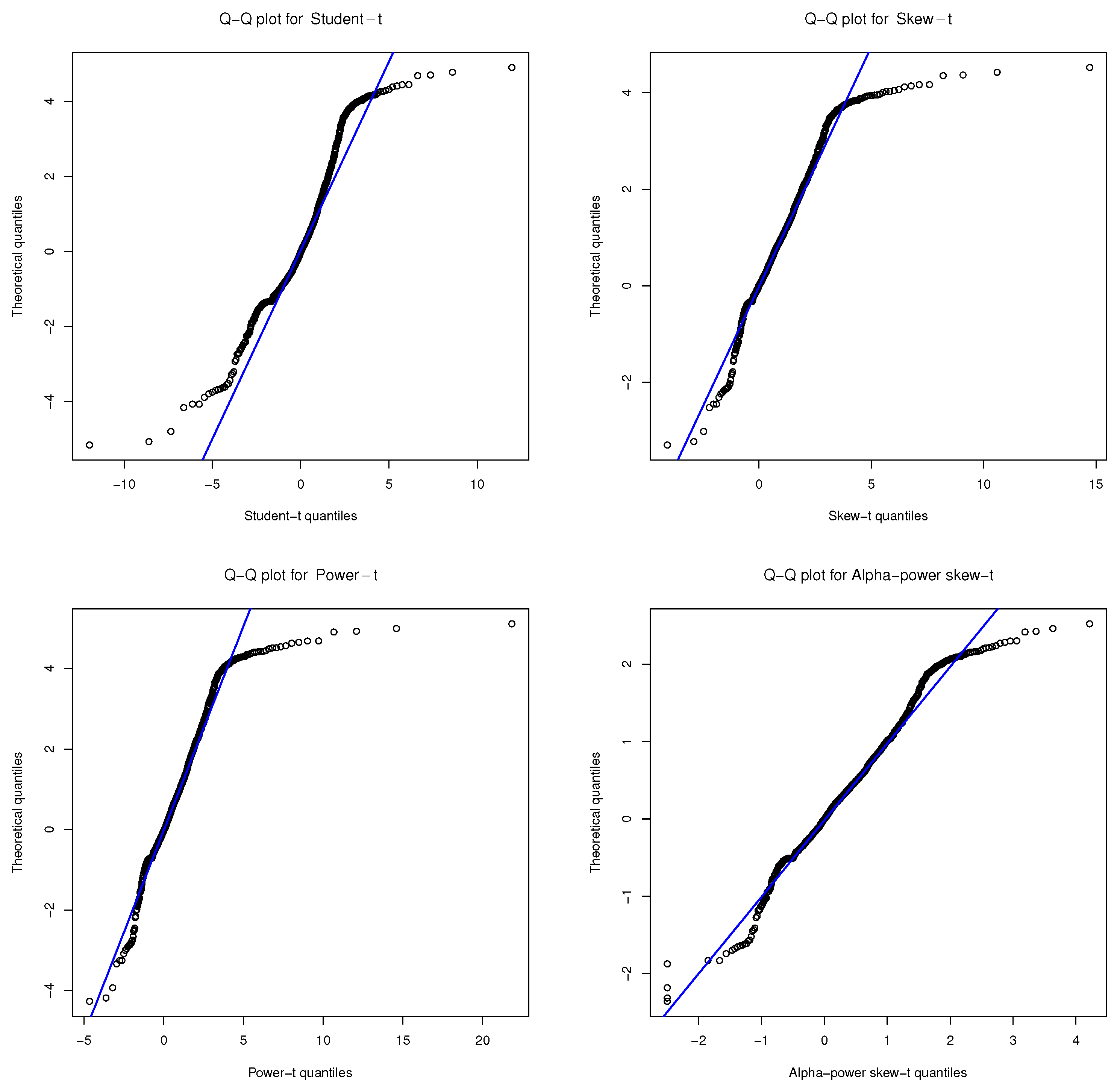
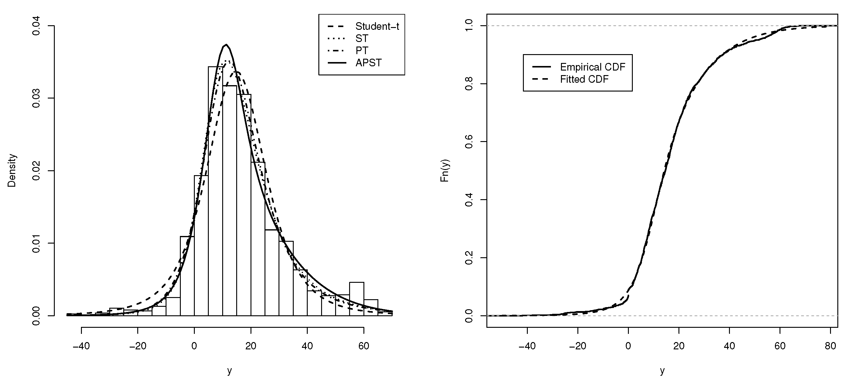
4.1. Application 1: Volcano Heights Data

Consider the data set related to heights of 1520 volcanoes in the world which is available in website dx.doi.org/10.5479/si.GVP.VOTW4-2013 [23]. Table 2 presents the summary statistics for the data set. It can be noted that the asymmetry and kurtosis indices seem to indicate that the use of an asymmetric and heavy-tailed model is appropriate to analyze this data set. We analyzed these data by fitting the Student-t, ST, PT, and APST distributions.

Table 2. Volcano heights data: Statistical summary.

n	Mean	Variance	$\sqrt{{\mathit{b}}_1}$	${\mathit{b}}_2$
1520	16.7760	15.6682	0.6461	4.3809

Table 3 shows the parameter estimates, together with their corresponding standard errors (SE). Note that the values of the standard errors of the $\mu$ and $\sigma$ estimates for the APST model are smaller than the corresponding standard errors of the respective parameters for the Student-t, ST, and PT models. Table 3 also presents some model selection criteria, together with the values of the log-likelihood. The AIC, BIC, and CAIC criteria indicate that the APST model seems to provide better fit to the volcanoes heights data than the T, ST, and PT models, supporting the asymmetry assertion of the volcano’s heights variable. Figure 2 shows the graphs QQplot of the fitted models. It can be clearly seen from the figure that the APST model fits the data better than the Student-t, ST, and PT models. In addition, we can use the likelihood ratio (LR) test statistic to conform our claim. To do this, we consider the following hypotheses,

$$H_0:(\lambda ,\alpha )=(0,1)(\mathrm{T}(\mu ,\sigma ,\nu ))\mathrm{v}.\mathrm{s}{H}_1:(\lambda ,\alpha )\ne (0,1)(\mathrm{APST}(\mu ,\sigma ,\lambda ,\alpha ,\nu )),$$

Table 3. Parameter estimates (SE) for the fitted models to the volcano height data.

	Distribution
Estimates	Student-t	ST	PT	APST
$\widehat{\mu }$	14.7835(0.3615 )	4.7469(0.6892)	8.4027(0.7923)	11.5509(0.1337)
$\widehat{\sigma }$	11.0045(0.3975)	14.1532(0.7237)	11.8146(0.4707)	22.6885(0.0792)
$\widehat{\lambda }$	–	1.5673(0.1838)	–	5.2347(0.2870)
$\widehat{\alpha }$	–	–	1.7912(0.1147)	0.3205(0.0347)
$\widehat{\nu }$	3.4156(0.3601)	3.4075(0.3454)	2.7473(0.2566)	12.8734(2.9729)
$\widehat{\ell }$	−6273.35	−6219.25	−6228.77	−6205.94
AIC	12,552.70	12,446.49	12,465.53	12,421.87
BIC	12,568.68	12,467.79	12,486.53	12,448.50
CAIC	12,571.68	12,471.79	12,490.83	12,453.50

Figure 2. Volcano height data: QQplot for Student-t, ST, PT, and APST models.

The value of the LR test statistic is $-2log(\Lambda )=-2\left({\ell }_T(\widehat{\theta })-{\ell }_{APST}(\widehat{\theta })\right)=$134.823 and comparing this quantity with ${\chi }_2^2=$5.9914, the null hypotheses is rejected. The APST model is also compared with the ST and PT models by considering the hypotheses

$$H_{01}:\alpha =1(\mathrm{ST}(\mu ,\sigma ,\lambda ,\nu ))\mathrm{v}.\mathrm{s}{H}_{11}:\alpha \ne 1(\mathrm{APST}(\mu ,\sigma ,\lambda ,\alpha ,\nu )),$$

and

$$H_{02}:\lambda =0(\mathrm{PT}(\mu ,\sigma ,\alpha ,\nu ))\mathrm{v}.\mathrm{s}{H}_{12}:\lambda \ne 0(\mathrm{APST}(\mu ,\sigma ,\lambda ,\alpha ,\nu )),$$

respectively. The respective values of the LR test statistic are given by $-2log({\Lambda }_1)=-2\left({\ell }_{ST}(\widehat{\theta })-{\ell }_{APST}(\widehat{\theta })\right)=$26.620 and $-2log({\Lambda }_2)=-2\left({\ell }_{PT}(\widehat{\theta })-{\ell }_{APST}(\widehat{\theta })\right)=$45.660 and comparing these quantities with ${\chi }_1^2=$3.8414, both null hypotheses are rejected. Finally, Figure 3left shows the histogram of the volcano heights variable, whereas Figure 3right presents the empirical CDF (solid line) together with the CDF of the fitted APST model (dotted line).

Figure 3. (Left) Graph of fitted densities to volcano height data. (Right) Empirical CDF and CDF of fitted APST model.

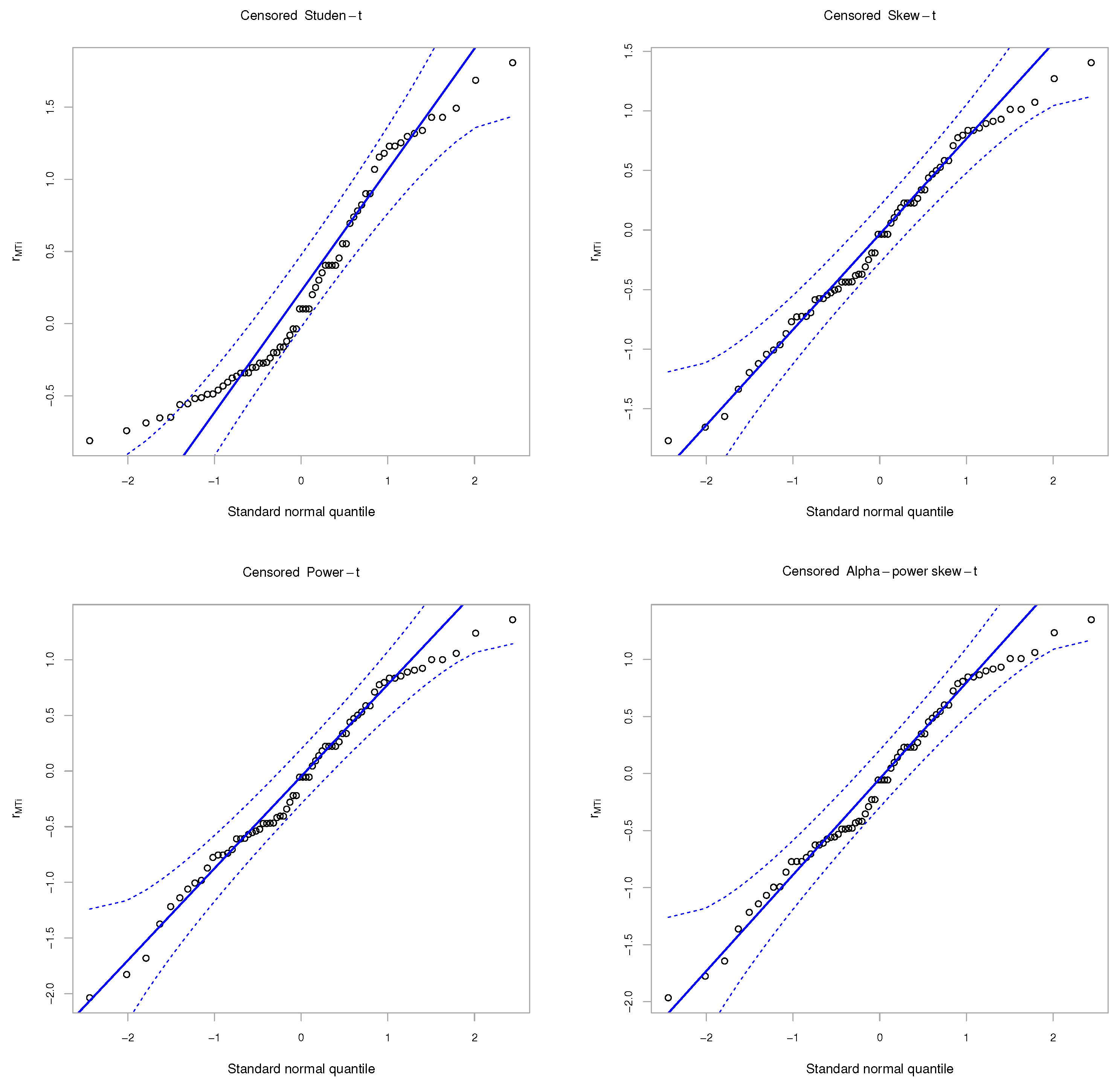
4.2. Application 2: Stellar Abundances Data

The second data set is related to measurements for 68 solar-type stars, which are available in the package astrodatR of the software R [24] under the name Stellar abundances. These data were previously analyzed Mattos et al. [25] by using the Scale Mixture of Skew Normal Censored Regression (SMSNCR) models. We take only the response variable: log N(Be), which represents the log of the abundance of beryllium scaled to Sun’s abundance (i.e., the Sun has $logN(Be)=0.0$)

In astronomical research, a previously identified sample of objects (stars, galaxies, quasars, X-ray sources, etc.) is observed at some new wavebands. According to Feigelson [24], due to limited sensitivities, some objects may be undetected, leading to upper limits in their derived luminosities. For this dataset we have 12 left-censored data points, i.e., 12 undetected beryllium measurement, that represents 19.35% of observations. Table 4 presents the ML estimates for the parameters of the censored Studen-t (CT), censored skew-t (CST), censored power-t (CPT), and censored alpha-power skew-t (CAPST) models, together with their corresponding standard errors. Table 4 also compares the fit of the four models using the model selection criteria (AIC, CAIC and BIC). Note that, again, the CAPST model with heavy tails have better fit than the CT, CST, and CPT models.

Table 4. Parameter estimates (SE) for the fitted models to the stellar abundances data.

	Distribution
Estimates	CT	CST	CPT	CAPST
$\widehat{\mu }$	1.0314(0.0010)	1.2306(0.0018)	1.2098(0.0052)	1.1761(0.0054)
$\widehat{\sigma }$	0.1596(0.0012)	0.2712(0.0058)	0.0818(0.0008)	0.0905(0.0020)
$\widehat{\lambda }$	–	−3.5655(3.7748)	–	0.6580(0.5031)
$\widehat{\alpha }$	–	–	0.1705(0.0208)	0.1518(0.0251)
$\widehat{\nu }$	0.9974(0.0884)	1.2501(0.1774)	6.0927(0.7501)	6.0999(0.7326)
$\widehat{\ell }$	−29.50743	−18.87016	−17.67113	−14.80241
AIC	65.01487	45.74033	43.34227	39.60482
BIC	71.67339	54.61836	52.22030	50.70236
CAIC	59.38987	38.37525	35.97719	30.57256

To identify atypical observations and/or model mispecification, we analyzed the transformation of the martingale residual, $r_{M{T}_i}$, proposed in Barros et al. [26]. These residuals are defined by

$$r_{MTi}=\mathrm{sign}(r_{Mi})\sqrt{-2[r_{Mi}+{\delta }_{i}log({\delta }_i-r_{M_i})]},i=1,\cdots ,n$$

where $r_{Mi}={\delta }_i+logS(y_i;\widehat{\mathit{\theta }})$ is the martingal residual proposed by Ortega et al. [27], where ${\delta }_i=0,1$ indicates whether the i-th observation is censored or not, respectively; $\mathrm{sign}(r_{Mi})$ denotes the sign of $r_{Mi}$; and $S(y_i;\widehat{\mathit{\theta }})=P_{\widehat{\mathit{\theta }}}(Y_i>y_i)$ represents the survival function evaluated at $y_i$, where $\widehat{\mathit{\theta }}$ are the MLE for $\mathit{\theta }$. The plots of $r_{M{T}_i}$ with generated confidence envelopes are presented in Figure 4. From this figure, we can see clearly that the CST, CPT, and CAPST models fit better the data than the CT model, since, in that cases, there are not observations which lie outside the envelopes. The Figure 5 shows the graph of the densities of the different models fitted to the stellar abundances data. From the figure, the CAPST model seems to fit better the stellar abundances data than CT, CST and CPT models.

Figure 4. Stellar abundances data. Envelopes of transformed martingale residuals for CT, CST, CPT, and CAPST models.

Figure 5. Graph of fitted densities to stellar abundances data.

5. Conclusions

In this work, a new asymmetric model has been introduced. It is based on the combination of skew-t [1] and power-t [2] models. The new model presents greater ranges of asymmetry and kurtosis, which is very useful for modeling skewed and heavy-tailed data. The problem of estimating the parameters in the model is dealt by using the maximum likelihood approach which is also used for developing large sample properties for the estimators. The elements of the observed information matrix are analytically obtained. The likelihood ratio statistics can be used for testing the APST null hypothesis since the Student-t, ST, and PT models are special cases of the model entertained. Two applications to volcano heights data and stellar abundances data indicate that the proposed model can be a useful alternative to the ST and PT models.

References

- Azzalini, A. A class of distributions which includes the normal ones. Scand. J. Stat. 1985, 12, 171–178. [Google Scholar]
- Durrans, S.R. Distributions of fractional order statistics in hydrology. Water Resour. Res. 1992, 28, 1649–1655. [Google Scholar] [CrossRef]
- Martínez-Flórez, G.; Bolfarine, H.; Gómez, H.W. The alpha–power tobit model. Commun. Stat. Theory Methods 2013, 42, 633–643. [Google Scholar] [CrossRef]
- Birnbaum, Z.W.; Saunders, S.C. A new family of life distributions. J. Appl. Probab. 1969, 6, 319–327. [Google Scholar] [CrossRef]
- Martínez-Flórez, G.; Bolfarine, H.; Gómez, H.W. An alpha-power extension for the Birnbaum-Saunders distribution. Statistics 2014, 48, 896–912. [Google Scholar] [CrossRef]
- Gupta, R.D.; Gupta, R.C. Analyzing skewed data by power-normal model. Test 2008, 17, 197–210. [Google Scholar] [CrossRef]
- Pewsey, A.; Gómez, H.W.; Bolfarine, H. Likelihood–based inference for power distributions. Test 2012, 21, 775–789. [Google Scholar] [CrossRef]
- Martínez-Flórez, G.; Bolfarine, H.; Gómez, H.W. Skew-normal alpha-power model. Stat. J. Theor. Appl. Stat. 2014, 48, 1414–1428. [Google Scholar] [CrossRef]
- Azzalini, A.; Capitanio, A. Distributions generated by perturbation of symmetry with emphasis on a multivariate skew-t distribution. J. R. Stat. Soc. Ser. B (Stat. Methodol.) 2003, 65, 367–389. [Google Scholar] [CrossRef]
- Branco, M.D.; Dey, D.K. General class of multivariate skew-elliptical distributions. J. Multivar. Anal. 2001, 79, 99–113. [Google Scholar] [CrossRef]
- Durrans, S.R. Multivariate skew t-distribution. Stat. J. Theor. Appl. Stat. 2003, 37, 359–363. [Google Scholar]
- Sahu, S.K.; Dey, D.K.; Branco, M.D. A new class of multivariate skew distributions with applications to Bayesian regression models. Can. J. Stat. 2003, 31, 129–150. [Google Scholar] [CrossRef]
- Jones, M.C.; Faddy, M.J. A skew extension of the t-distribution, with Applications. J. R. Stat. Soc. Ser. B (Stat. Methodol.) 2003, 65, 159–174. [Google Scholar] [CrossRef]
- Zhao, J.; Kim, H.M. Power t distributions. Commun. Stat. Appl. Methods 2016, 23, 321–334. [Google Scholar]
- R Development Core Team. R: A Language and Environment for Statistical Computing; R Foundation for Statistical Computing: Vienna, Austria, 2018; Available online: http://www.R-project.org (accessed on 10 October 2019).
- Lehman, E.L.; Casella, G. Theory of Point Estimation, 2nd ed.; Springer: New York, NY, USA, 1998. [Google Scholar]
- Frieden, B.R. Science from Fisher Information: A Unification; Cambridge Univerisity Press: Cambridge, UK, 2004. [Google Scholar]
- Arellano-Valle, R.B.; Azzalini, A. The centered parameterization and related quantities of the skew–t distribution. J. Multivar. Anal. 2013, 113, 73–90. [Google Scholar] [CrossRef]
- Arellano-Valle, R.B.; Azzalini, A. The centered parametrization for the multivariate skew-normal distribution. J. Multivar. Anal. 2008, 99, 1362–1382. [Google Scholar] [CrossRef]
- Akaike, H. A new look at statistical model identification. IEEE Trans. Autom. Contr. 1974, 19, 716–722. [Google Scholar] [CrossRef]
- Schwarz, G. Estimating the dimension of a model. Ann. Stat. 1978, 6, 461–464. [Google Scholar] [CrossRef]
- Bozdogan, H. Model selection and akaike’s information criterion (AIC): The general theory and its analytical extensions. Psychometrika 2010, 52, 345–370. [Google Scholar] [CrossRef]
- Siebert, L.; Simkin, T.; Kimberly, P. Global Volcanism Program. In Volcanoes of the World; v. 4.6.0.; Venzke, E., Ed.; Smithsonian Institution: Washington, DC, USA, 2013; Available online: https://doi.org/10.5479/si.GVP.VOTW4-2013 (accessed on 10 October 2019).
- Feigelson, E.D. astrodatR: Astronomical Data. R Package v. 0.1. Available online: http://CRAN.R-project.org/package=astrodatR (accessed on 10 October 2019).
- Mattos, T.; Garay, A.M.; Lachos, V.H. Likelihood-based inference for censored linear regression models with scale mixtures of skew-normal distributions. J. Appl. Stat. 2018, 45, 2019–2066. [Google Scholar] [CrossRef]
- Barros, M.; Galea, M.; González, M.; Leiva, V. Influence diagnostics in the tobit censored response model. Stat. Methods Appl. 2010, 19, 379–397. [Google Scholar] [CrossRef]
- Ortega, E.M.; Bolfarine, H.; Paula, G.A. Influence diagnostics in generalized log-gamma regression models. Comput. Stat. Data Anal. 2003, 42, 165–186. [Google Scholar] [CrossRef]
© 2020 by the authors. Licensee MDPI, Basel, Switzerland. This article is an open access article distributed under the terms and conditions of the Creative Commons Attribution (CC BY) license (http://creativecommons.org/licenses/by/4.0/).