Article

Automatic Retinal Blood Vessel Segmentation Based on Fully Convolutional Neural Networks

College of Computer Science and Engineering, Northwest Normal University, Lanzhou 730070, China
*
Author to whom correspondence should be addressed.
These authors contributed equally to this work.
Symmetry 2019, 11(9), 1112; https://doi.org/10.3390/sym11091112
Submission received: 24 July 2019 / Revised: 26 August 2019 / Accepted: 27 August 2019 / Published: 3 September 2019
(This article belongs to the Special Issue Advances in Medical Image Segmentation 2019)

Abstract

:
Automated retinal vessel segmentation technology has become an important tool for disease screening and diagnosis in clinical medicine. However, most of the available methods of retinal vessel segmentation still have problems such as poor accuracy and low generalization ability. This is because the symmetrical and asymmetrical patterns between blood vessels are complicated, and the contrast between the vessel and the background is relatively low due to illumination and pathology. Robust vessel segmentation of the retinal image is essential for improving the diagnosis of diseases such as vein occlusions and diabetic retinopathy. Automated retinal vein segmentation remains a challenging task. In this paper, we proposed an automatic retinal vessel segmentation framework using deep fully convolutional neural networks (FCN), which integrate novel methods of data preprocessing, data augmentation, and full convolutional neural networks. It is an end-to-end framework that automatically and efficiently performs retinal vessel segmentation. The framework was evaluated on three publicly available standard datasets, achieving F1 score of 0.8321, 0.8531, and 0.8243, an average accuracy of 0.9706, 0.9777, and 0.9773, and average area under the Receiver Operating Characteristic (ROC) curve of 0.9880, 0.9923 and 0.9917 on the DRIVE, STARE, and CHASE_DB1 datasets, respectively. The experimental results show that our proposed framework achieves state-of-the-art vessel segmentation performance in all three benchmark tests.

1. Introduction

Some pathological diseases in the human body can be detected through changes in the morphology and morphology of retinal vessels. Therefore, the condition of the retinal vessels is an important indicator for the diagnosis of some retinal diseases. For example, the progression of diabetic retinopathy is the most life-threatening because it leads to vision loss due to high sugar levels and hypertension in later stages [1]. Doctors can detect other diseases of the body in advance by examining some eye diseases and make an early diagnosis of these diseases to carry out the corresponding treatment in advance. According to reports, early detection, timely treatment, and appropriate follow-up procedures can prevent about 95% of blindness [1].
Because the retinal vessels are easily photographed, the surgeon uses a retinal camera to acquire the retinal image of the patient. Fundus vessels are the most stable and important structures with symmetrical and asymmetrical patterns that are detectable. When the visual organ disease occurs in the eye, the diameter, color, and bending degree of the retinal blood vessel may be abnormal. Usually, the ophthalmologist manually performs blood vessel segmentation from the retinal image to extract lesion information. However, this work is cumbersome, error-prone, and time-consuming, even for experienced doctors [2]. Therefore, automatic and accurate segmentation is essential. Currently, relatively new technology is the introduction of computer-aided diagnosis, which can provide more objective and accurate diagnosis results and improve the diagnostic efficiency of doctors. Automated fundus vessel segmentation technology is able to identify and extract related symmetrical and asymmetrical patterns, which are essential and valuable for medical diagnosis of eye diseases. With the continuous development of computer vision technology, many methods for fundus vascular analysis have been proposed in recent decades. In essence, they can be classified into supervised and unsupervised algorithms.
Unsupervised methods determine whether a pixel is a blood vessel by extracting symmetric and asymmetrical patterns of blood vessels in the fundus. It can be further classified into five main subcategories: matched filtering, morphological processing, vessel tracking, multiscale analysis, and model-based algorithms. The 2D kernel is convolved with the retinal image in a matched filtering method, and the matched filter response indicates the presence of the feature. A threshold probing technique on a matched filter response image was presented by Hoover et al. [3], and they combined local and region-based properties of the vessels for segmentation. A combined matched filter, Frangi filter, and Gabor Wavelet filter were used to enhance blood vessel in [4]. They also use the average of some performance indicators to enhance the contrast between the blood vessels and the background. The method proposed by Zardadi et al. [5] enhances the blood vessels in various directions. They classify each pixel via an adaptive thresholding algorithm and then perform morphological post-processing. However, several spots were incorrectly segmented into blood vessels, which affected the final performance of the algorithm. In [6], vessel centerlines detection and morphological bit plane slicing are combined to extract vessels from the retinal image. A method of combining blood vessels and k-means clustering to segment blood vessels was proposed in [7], but the use of this method for vessels of various width may result in the loss of the tiny structures. Vessel tracking algorithm uses local information to segment the blood vessels between two points and work at the level of a single vessel [8]. In [9], a set of points (manual or automatic selection) is established, and the vessel centerline is iteratively followed to extract the vessel tree. However, besides being poor at detecting not seeded vessel segments, they may also miss the originally labeled vessel segment.
Unsupervised methods can perform blood vessel segmentation tasks on large amounts of unlabeled data. However, there are some problems with the unsupervised method compared with a supervised method. Due to noise and pathological patterns, the performance and generalization of unsupervised methods are not very good. For example, when there is a lesion in the fundus image, the segmentation result of the matched filtering method will be very poor. The matched filtering method is more suitable for the screening of healthy fundus images, which is far from enough. The vascular tracking method is capable of accurately marking the width of a blood vessel, but cannot detect retinal blood vessels without a seed point.
Supervised methods utilizing ground truth data for vessel segmentation contain two steps: (1) feature extraction and (2) classification. Many methods have been proposed to handle different supervised segmentation tasks such as K-nearest neighbor (KNN) [10], support vector machine (SVM) [11], or convolutional neural network (CNN) [12]. In [13], the hybrid feature vectors calculated by the different extractors are used to characterize the pixels and then classified using a random forest classifier. In [14], an ensemble system of bagged and boosted decision trees based on gradient vector field, morphological transformation, line strength measurement, and Gabor filter response was proposed. In recent years, some studies have investigated the problem of blood vessel segmentation based on deep learning. A deep learning method based on fully convolutional neural network (FCN) for a holistically-nested edge detection problem is developed in [15]. A CNN that automatically, simultaneously segments and discrimination exudates, hemorrhages and micro-aneurysms were proposed in [12]. In [16], multi-scale hierarchical features of different receptive fields are proposed to achieve better performance. This method can handle the change of receptive field size required by different regions. In [17], a deep learning method combining holistically-nested edge detection and conditional random field is proposed. There are still some problems with supervised methods. Many studies have preprocessed images based on experience, but little research has been done on preprocessing methods. Data augmentation methods can improve the generalization ability and performance of CNN. However, existing data augmentation methods are not necessarily applicable to retinal blood vessel images. Moreover, the existing methods still have problems such as low segmentation accuracy and poor generalization. The existence of these problems has become the main motivation for this research.
In this paper, we have devised a new automatic segmentation framework for retinal vessels based on deep fully convolutional neural networks (FCN). Our specific contributions are as follows:
(1)
We delved into the effects of several data preprocessing methods on network performance. By performing grayscale, normalization, Contrast Limited Adaptive Histogram Equalization (CLAHE), and gamma correction on the retina image, the performance of the model can be improved.
(2)
We have devised a new data augmentation method for retinal images to enhance the performance of the model. It can be combined with existing data augmentation methods to achieve better results. We named it Random Crop and Fill (RCF).
(3)
We proposed M3FCN, an improved deep fully convolutional neural network structure, for retinal vessel automatic segmentation. Compared with the basic FCN, the M3FCN has the following three improvements: adding a multi-scale input module, expanding to a multi-path FCN, and obtaining the final segmentation result through multi-output fusion. The experimental results show that all three improvements can improve the performance of the model.
(4)
We obtain the final segmentation image by overlapping the sampling test patch and the overlapping patch reconstruction algorithm.
(5)
We have proved through the ablation analysis experiments that the various improvements proposed in this paper are effective. Experimental results show that the proposed framework is robust and that the improved method has the potential to extend to other methods and medical images.
We tested the proposed framework on three standard retinal image datasets: DRIVE [10], STARE [3], and CHASE_DB1 [18]. The proposed automatic retinal vascular segmentation framework can achieve state-of-the-art results, which prove the robustness and effectiveness of the method. The contributions of this paper also include retinal image preprocessing methods and new data augmentation methods. These methods will also benefit other vessel segmentation tasks.

2. Methodology

The new retinal vessel segmentation framework is shown in Figure 1, which consists of two stages. The first stage is the training stage, which consists of the following four steps: (1) preprocessing the retinal images; (2) extracting the patches by the dynamic extraction patch strategy; (3) inputting the patches to the fully convolutional neural network to extract features and classifications; (4) updating the network weights by the mini-batch Gradient Descent method and the backpropagation algorithm. The second stage is the testing stage, which also includes four steps: (1) the same data preprocessing method is used to process the test image; (2) the overlapping extraction patch method is used to extract the patches; (3) the patches are input to the fully convolutional neural network to extract features and classified to obtain segmentation patches; (4) the segmentation patches are reconstructed into target segmentation images by the overlap patch reconstruction algorithm.

2.1. Materials

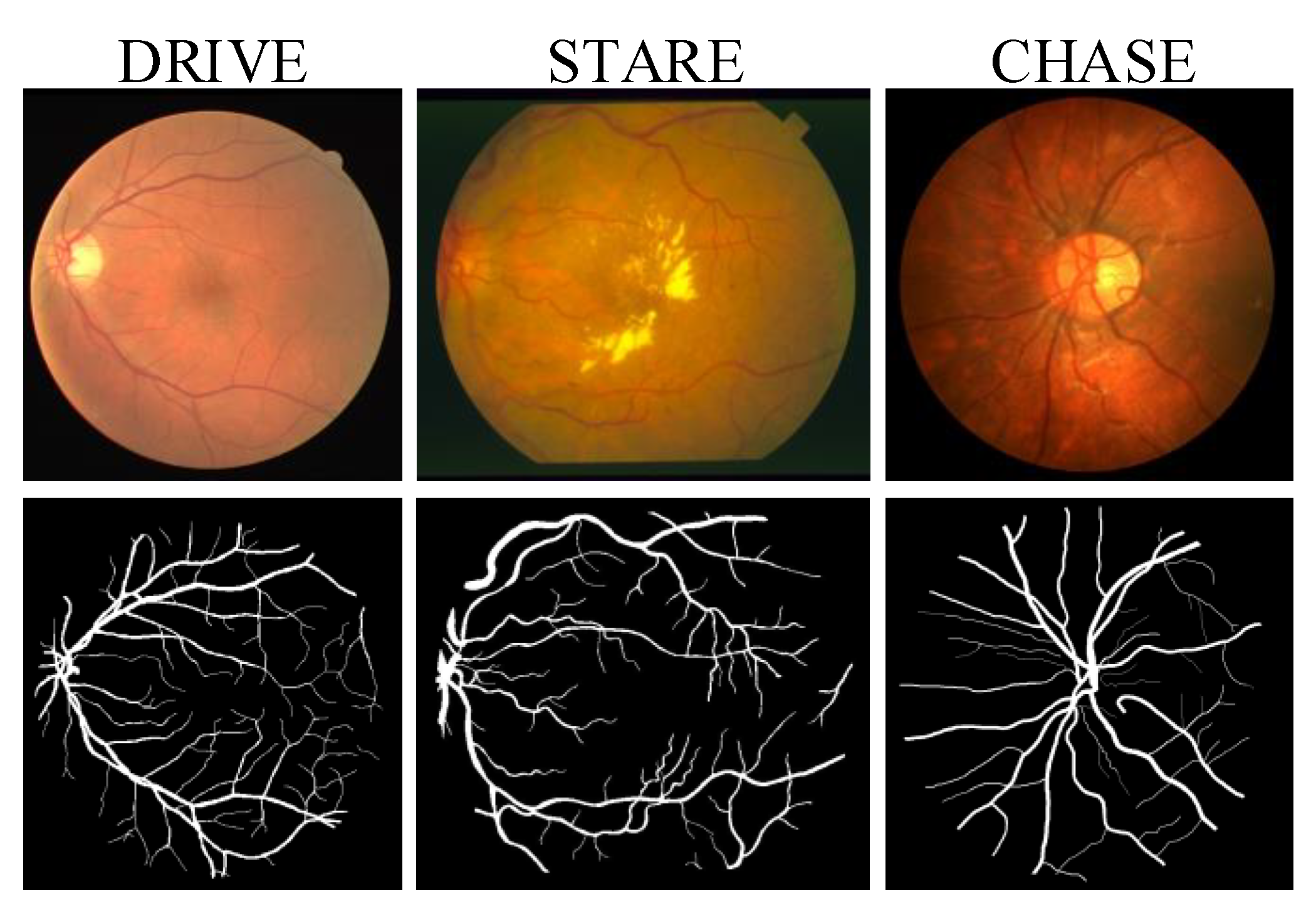
Performances are evaluated on three public datasets: Digital Retinal Images for Vessel Extraction (DRIVE) [10], Structured Analysis of the Retina (STARE) [3], and CHASE_DB1 (CHASE) [18]. Retinal images in three datasets were obtained under different equipment, illumination, etc. The DRIVE dataset contains 40 retinal images with a resolution of 565 × 584 px, 20 of which are used for training and the rest for testing. The STARE dataset has 20 retina images with a resolution of 700 × 605 px, 10 of which are lesions. The CHASE dataset consists of 28 retina images with a resolution of 999 × 960  px. Figure 2 shows an example of different datasets. All datasets provide segmentation results for two experts. We use the first expert results as ground truths and compare our segmentation results with the second expert results.

2.2. Dataset Preparation and Image Preprocessing

2.2.1. Dataset Preparation

All datasets are divided into training sets for training networks and test sets for performance evaluation. For DRIVE, we follow the criteria given by the data publisher, with 20 images for training and the remaining 20 images for testing. Similar data partitioning strategy was not initially provided for the STARE and CHASE datasets. For STARE, we used the ‘leave-one-out’ method proposed by [2,19,20], which is trained on 19 samples and tested on the remaining one iteratively. For CHASE, we adopted the split strategy proposed by [21], which is trained on 20 images and tested on the remaining eight images (from four children).

2.2.2. Image Preprocessing

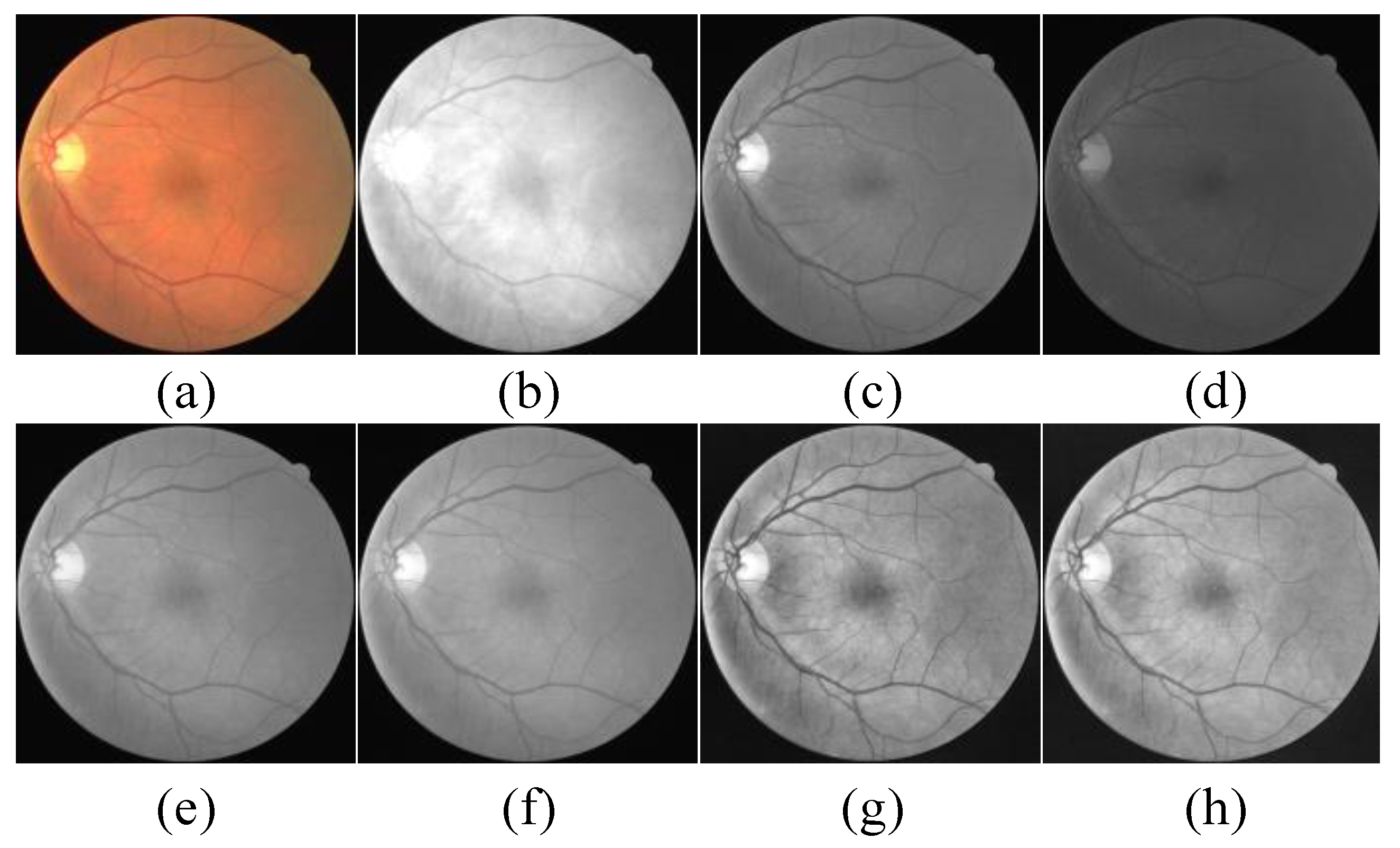
After proper preprocessing of the image, the deep neural network can learn the image data distribution more effectively. Four image preprocessing strategies were used in our proposed framework to preprocess the images in sequence. Figure 3 shows the image after each preprocessing strategy.
The first preprocessing strategy is to convert RGB images into single-channel grayscale images. Figure 3a–d shows that the original image and the converted single-channel grayscale image are red, green, and blue, respectively. By decomposing the RGB color image into three-channel monochrome images of red, green and blue, it can be seen that there is a higher degree of discrimination between the blood vessels and the background in the green channel, and the monochrome image of the red and blue channels has more noise and low contrast. Single-channel grayscale image shows better vessel background contrast than RGB images [19]. Therefore, the original RGB image is converted into a single-channel grayscale image by [22]. The conversion formula is as follows:
I g r a y = 0.299 × r + 0.587 × g + 0.114 × b ,
where r, g, b are the red, green and blue channels, respectively. According to this equation, red, green and blue contribute 29.9%, 58.7% and 11.4% respectively, of which green is greater in all three colors. The grayscale image is shown in Figure 3e.
The second preprocessing strategy is data normalization. Normalizing the image can improve the convergence speed of the model [23]. Let X = { x 1 , x 2 , , x n } be the image dataset. Z-score normalization [24] refers to setting each dimension of the data X to have zero-mean and unit-variance. The conversion formula is as follows:
X n o r m = X μ σ ,
where μ and σ are the mean and standard deviation of X, respectively. Image data are mapped to a range of 0 to 255 by Min-Max scaling. The conversion formula is as follows:
x i = x i x m i n i x m a x i x m i n i ,
where x i X n o r m , i [ 1 , 2 , , n ] . The normalized image is shown in Figure 3f.
The third preprocessing strategy is to enhance the foreground-background contrast of the whole dataset using Contrast Limited Adaptive Histogram Equalization (CLAHE) [25]. The CLAHE image is shown in Figure 3g. The last preprocessing strategy is to improve the image quality much further using gamma correction. In our experiments, the gamma value is set to 1.2 . The gamma correction image is shown in Figure 3h. We implement the CLAHE and gamma correction function using OpenCV [26].

2.3. Dynamic Patch Extraction

A large number of images are often required to train the convolutional neural network, which can reduce over-fitting risk and improve model performance. However, the number of existing retinal image datasets is insufficient to support the training model. Inspired by [2,19,21,27], in our approach, patch-based learning strategies get patches differently that are fed to the network, depending on the stage of the framework. To solve the problem of insufficient memory during training, we dynamically extract a small number of patches in the loop training. Algorithm 1 describes the process of training FCN with a dynamic extraction patch strategy.
Algorithm 1 Training FCN with dynamic extraction patch strategy
Input: Train images X R N × 1 × H × W , ground truths G R N × 1 × H × W .
Input: Patch size p, dynamic patch number n.
Input: Initial FCN parameter θ , epochs E.
Output: FCN parameter θ .
 Initialize patch images I R n × 1 × p × p .
 Initialize patch labels T R n × 1 × p × p .
for e = 1 to E do
  for n = 1 to N do
   for k = 1 to n N do
    Randomly generate the center coordinates ( x , y ) of the patch.
    Patches I and labels T are extracted from X and G centered on ( x , y ) , respectively.
   end for
  end for
   l o s s = 1 n θ i n L ( f ( I [ i ] ; θ ) , T [ i ] ) .
  Update parameters θ using the Adam [28] optimizer.
end for
return θ .
During the test stage, the test set images are progressively oversampled. Let W, H be the image width and height. Let p be the patch size. Let s be the overlap sampling step size. Then, the number of patches per test image is:
N = H p s × W p s .
We oversample the testset image and use it as input to the model to obtain the corresponding segmented image. Finally, the segmentation images are reconstructed into the retina segmentation image by the overlap patch reconstruction algorithm. Algorithm 2 describes the process of testing FCN with the overlapping patches reconstruction algorithm.
Algorithm 2 Testing FCN with overlapping patches reconstruction algorithm
Input: Test images X R N × 1 × H × W , patch size p, stride size s.
Output: Final segmentation result O .
N h = ( H p ) / S , N w = ( W p ) / S .
H = N h × p , W = N w × p .
 Zero padding for X to X R N × 1 × H × W .
 Initialize O p R N × 1 × H × W .
 Initialize O s R N × 1 × H × W .
for n = 1 to N do
  for h = 1 to N h do
   for w = 1 to N w do
    A patch x R 1 × 1 × p × p is extracted with ( h × s , w × s ) as the upper left coordinate.
    Input x into the trained FCN to get the output y.
    Assign y to the corresponding area of O p .
    Assign 1 to the corresponding area of O s .
   end for
  end for
end for
O = O p / O s .
 Crop O R N × 1 × H × W to get the final segmentation image O R N × 1 × H × W .
return O

2.4. A Novel Retinal Image Data Augmentation Method

Data augmentation is widely used in convolutional neural networks due to its effectiveness, scalability, and ease of implementation. Data augmentation operation of translating and rotating a few pixels of the training set image can generally improve the generalization ability of the model, reduce the risk of over-fitting, and improve the robustness of the model [29]. Commonly used data augmentation methods are rotation, flipping, cropping, adding noise, and translation. However, as explained in [27], methods such as continuous rotation make the network more difficult to detect blood vessel segments.
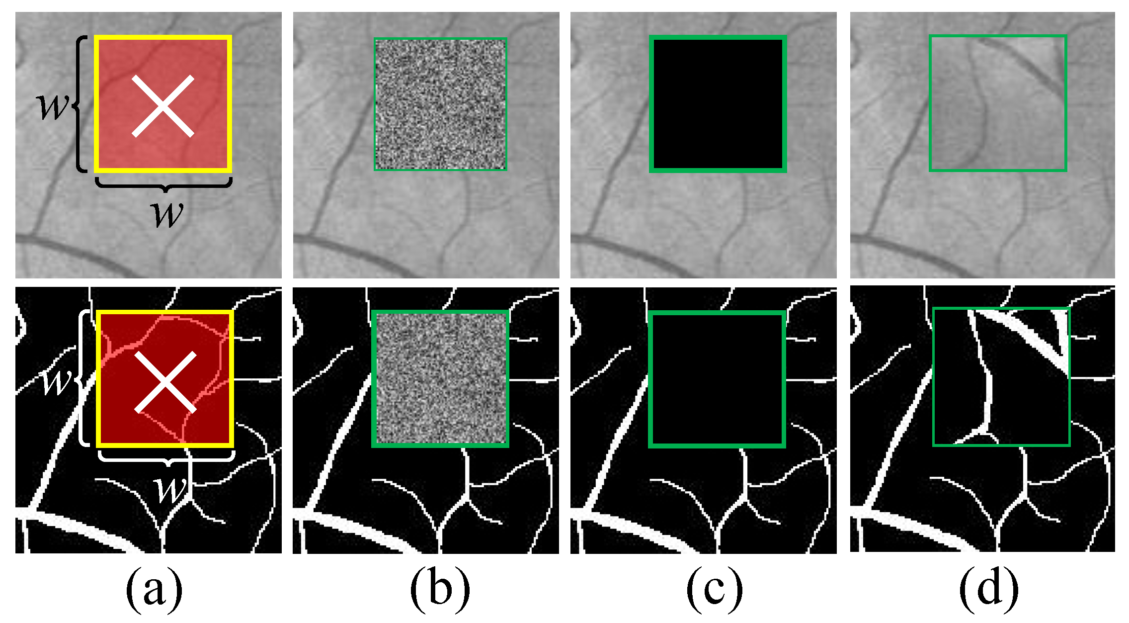
We have devised a new data augmentation method for retinal images to enhance the performance of the model. We call it Random Crop and Fill (RCF). We proposed a novel data augmentation method called Random Crop and Fill (RCF) for the retinal image. The conceptual explanation of RCF is shown in Figure 4. The core idea of the RCF is to transform the local area of the image by applying a fixed size mask to the random position of each input image during each training period. In general, we found that the size of the area is a hyper-parameter that is more important than the shape, so, for the sake of simplicity, we used square clipping areas for all experiments. It consists of two steps of data manipulation. Firstly, we randomly select one patch ( p × p ) from the training set and randomly select a point C ( x , y ) from the patch as the cropping center. Let the ratio of the width of the square clipping area to the width of the patch as R. The area centered at C and having a width w = p × R is cropped from the patch. Secondly, for the cropped area, we consider the following three ways to fill: (1) Assign a random value of [0,255] to each pixel, denoted as RCF-R; (2) Fill the deleted area with 0, denoted as RCF-0; (3) Randomly select another patch from the training set and select the value of the corresponding area to fill in the deleted area, denoted as RCF-A. The results of the filling are shown in Figure 4. To ensure that the network sometimes receives unmodified patches, we perform RCF transformation with a probability p. The RCF method is a lightweight calculation method. At the expense of minimal memory consumption and training time, the diversity of the dataset is greatly improved, without the need to add additional training parameters and without affecting test time. This method is a novel data augmentation for retinal images that work well with existing data augmentation methods.
On the other hand, we also use the data augmentation method to train FCN and discuss the association between RCF and data augmentation methods. We performed data augmentation in the following ways: (1) Randomly rotate 90 , 180 , 270 with 50% probability; (2) Random horizontal and vertical flip with 50% probability. These transformations are applied to the original patches and the ground truths.

2.5. Fully Convolutional Neural Network (FCN)

2.5.1. The Basic FCN Architecture

Our custom basic FCN implementation has an overall architecture similar to a standard FCN [30], as shown in Figure 5. Basic FCN include encoders and decoders symmetrically up and down the architecture. The encoding path is used to encode lower-dimensional input images with richer filters, capturing semantic/contextual information. The decoding path is designed to perform the inverse of the encoding and restore the spatial information by upsampling and fusion the low-dimensional features, which makes it possible to locate accurately. The difference between our custom basic FCN and the standard FCN is that we use the residual block [29] instead of one convolution layer. The shortcut connection in the residual block avoids the gradient disappearance problem of the CNN because the gradient of the residual block is always greater than or equal to 1 in back-propagation. Before each convolution layer, we use the batch normalization layer [23] to normalize the features so that they have a mean of 0 and a variance of 1. Using the BN layer can greatly improve the training speed and improve the stability and generalization of the model [23].

2.5.2. Multi-Scale, Multi-Path, and Multi-Output Fusion FCN (M3FCN)

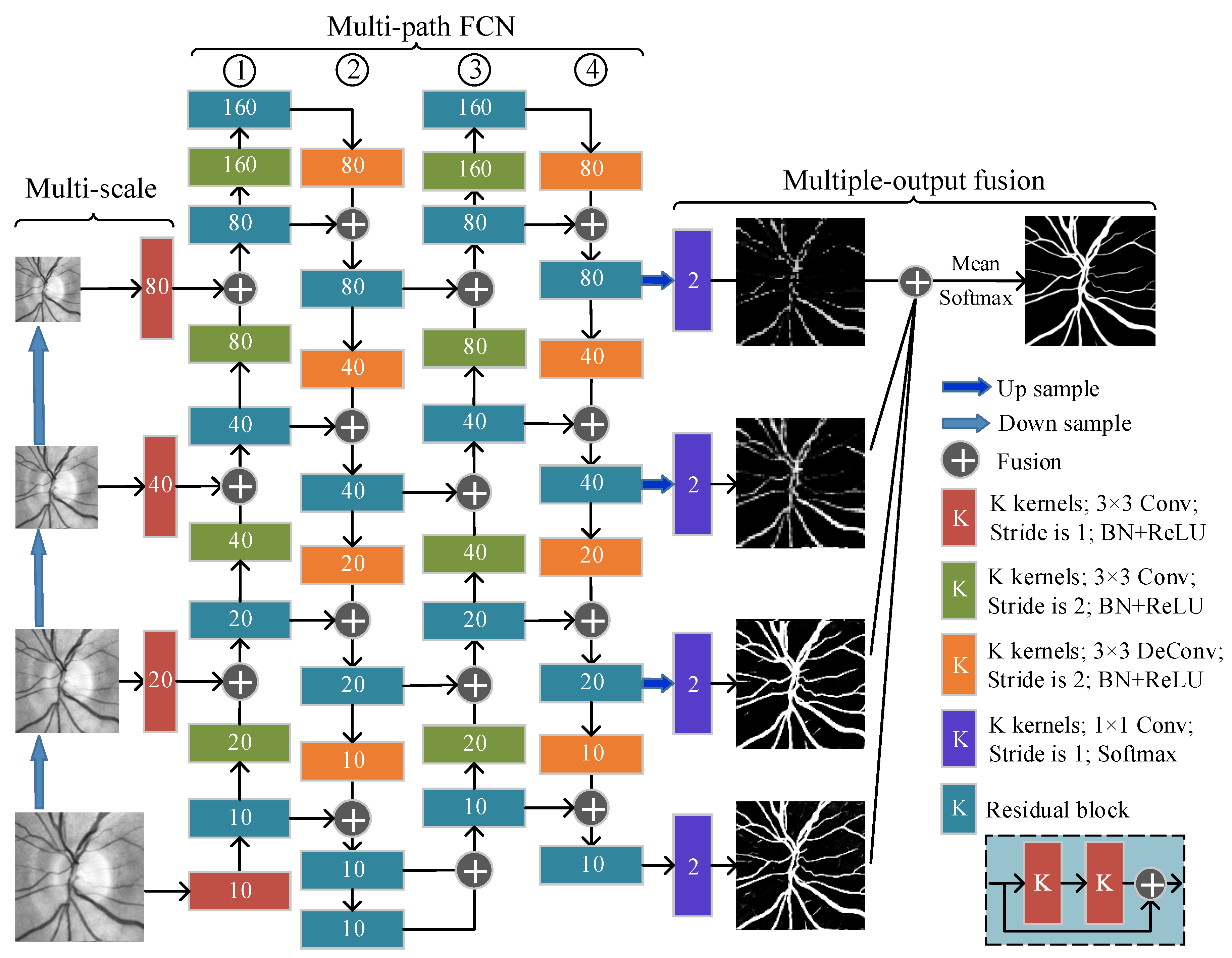
Inspired by the basic FCN, we proposed Multi-scale, Multi-path, and Multi-output fusion FCN (M3FCN) for retinal vessel segmentation tasks. Figure 6 illustrates the architecture of M3FCN. The M3FCN consists mainly of three improved parts. The first is the multi-scale layer, which is used to construct image pyramid input and achieve multi-level perceptual field fusion. This is followed by a multi-path FCN that is used as a subject structure to learn a rich hierarchical representation. The final is multi-output fusion, which is combined with low-level features with advanced features to support deep supervision.
(1) Multi-path FCN: Similar to the basic FCN architecture, M3FCN consists of two encoder paths (①, ③) and two decoder paths (②, ④). Each encoder path utilizes residual blocks and common convolutional layers to produce a set of encoder feature maps, and normalizes each layer feature map using the batch normalization layer and then activates them using the Leaky ReLU [31] activation function. Each decoder path decodes the features produced by the encoder using the deconvolution layer and the residual block, and normalizes each layer feature map using the batch normalization layer and then activates them using the ReLU [32] activation function. The skip connection fuses the feature map of the encoder with the feature map of the decoder.
(2) Multi-scale: The multi-scale inputs are integrated into the encoder path ① to ensure feature transfer of the original image and effectively improve segmentation quality. We downsample the image using the average pooling layer, then use the convolution to expand the channel of the downsampled image and build a multi-scale input in the encoder path ①.
(3) Multi-output fusion: In decoder path ④, we extract the output feature map of each residual block, use the upsampling method to extend the feature map to the input image size, and then input them to the classifier for classification. Finally, the probability maps obtained by different classifiers are fused as the final classification result. For the retinal blood vessel segmentation task, the output is a two-channel probability map, where the two channels are the class number for blood vessel and background, respectively.
The new model has been trained to combine low-level features with advanced features and adaptively train the receptive field and sampling position based on the proportion and shape of the vessel, both of which enable precise segmentation. Through this architecture, M3FCN can learn to distinguish features and generate accurate retinal blood vessel segmentation results.

3. Experimental Setup

3.1. Evaluation Metrics

We use several metrics to evaluate the performance, including F1 score, Accuracy, Sensitivity, Specificity, and area under the ROC curve (AUC). When these indicators reach 1, the model is best. Different metrics are calculated as follows:
A c c u r a c y = T P + T N T P + T N + F P + F N ,
S e n s i t i v i t y = T P T P + F N ,
S p e c i f i c i t y = T N T N + F P ,
P r e c i s i o n = T P T P + F P ,
R e c a l l = T P T P + F N ,
F 1 = 2 × P r e c i s i o n × R e c a l l P r e c i s i o n + R e c a l l ,
where T P is the correctly labeled blood vessel pixel. T N is the background pixel that is correctly marked. F P is the background pixel that is mislabeled. F N is a blood vessel pixel that is mislabeled.

3.2. Implementation Details

The hardware environment of our laptops includes NVIDIA GeForce GTX 1060 GPU, Intel Core i7-7700HQ [email protected] GHz processor, 32 GB of RAM, and running Linux Ubuntu OS 16.04. All training and testing were performed in the same hardware environment. We initialize the network according to the initialization method proposed by [33] and use the Adam optimizer [28] to train the network and use the Softmax function for the final classification. The learning rate and mini-batch size are 0.001 and 256, respectively. Binary segmentation is obtained by thresholding the probability map to 0.49. The stride size is 5. On the DRIVE dataset, the patch size is 48, and the number of patches is 100,000. On the STARE dataset, the patch size is 256, and the number of patches is 1900. On the CHASE dataset, the patch size is 128, and the number of patches is 12,800. For more details on implementation, please refer to our code and logs at https://github.com/HaiCheung/FCN. All code is implemented using Pytorch [34].

4. Results and Discussion

4.1. Ablation Analysis

4.1.1. Validation of the Image Preprocessing

We first evaluated the effect of the various steps involved in image preprocessing. The results for each variant are shown in Table 1. Comparing No. 0 with No. 1, it can be seen that, after conversion to a grayscale image, the experimental results are greatly improved compared with RGB color images, and the F1 score is increased by 1.06%. Therefore, subsequent experiments were performed using grayscale images. Comparing experiments with or without data normalization and CLAHE shows that these methods have a positive effect. When using gamma correction but not using CLAHE, performance is degraded, such as No. 4 and No. 6. It is worth noting that the combination of gamma correction and CLAHE is more efficient, such as No. 7 and No. 8. In particular, the F1 score reached 0.8321 when combined with these four preprocessing methods (No. 8), which was 2.73% higher than the baseline without any image preprocessing (No. 0). In the following experiment, we will continue to use these four preprocessing methods for experiments.

4.1.2. The Impact of RCF’s Hyper-Parameters

When implementing RCF on FCN training, we have three hyper-parameters to evaluate, i.e., the probability p, the width ratio R, and the filling method. To demonstrate the impact of these hyper-parameters on the model performance, we conduct experiments on DRIVE based on M3FCN under varying hyper-parameter settings. When evaluating one of the parameters, we fixed the other two parameters. The results are shown in Figure 7 and Table 2. In the experiments, we used data augmentation to compare the performance of the RCF method under different parameters. In particular, when p = 0 or R = 0 , it means using data augmentation but not using RCF and using this as our baseline. It can be seen from Figure 7 and Table 2 that, when p = 0.5 , R = 0.5 , and the filling method is RCF-A, M3FCN reaches the highest F1 score of 0.8321. Specifically, our best result increased the F1 score by 0.33% compared with the baseline. In the following experiment, we set p = 0.5 , R = 0.5 , and the filling method is RCF-A.

4.1.3. Validation of the Data Augmentation and RCF

To investigate the impact of data augmentation and RCF, we conducted experiments on the DRIVE based on M3FCN. The results for each variant are shown in Table 3. When applied alone, data augmentation ( F 1 = 0.8288 ) outperforms the RCF-A ( F 1 = 0.8255 ), but all outperforms the baseline ( F 1 = 0.8242 ). Importantly, RCF-A and the data augmentation methods are complementary. Particularly, the F1 score of 0.8321 can be obtained by combining these methods, which is 0.79% better than the baseline. In the following experiment, we will continue to use the data augmentation and RCF-A.

4.1.4. Comparisons with FCN and M3FCN

Compared to the basic FCN with M3FCN, M3FCN mainly has the following improvements: (1) adding multi-scale input modules; (2) expanding to multi-path FCN; and (3) using multi-output fusion to obtain final segmentation results. In order to analyze the effects of these improvements, we performed an ablation experiment: comparing improved and non-improved FCN performance based on equal experimental setups. We evaluated the model using the DRIVE test data. F1 score, Accuracy, Sensitivity, Specificity, and AUC were shown in Table 4. It can be concluded from Table 4 that the performance of M3FCN is better than other improved models. The global F1 score for basic FCN and M3FCN is 0.8279/0.8321 on DRIVE. According to Table 4, we can draw the following experimental summary: (1) M3FCN performs better than other improved models; (2) the performances with multi-path FCN are better than non-multipath FCN, which indicates that multi-path structure has better feature extraction and noise reduction; (3) multi-scale input or multi-output fusion combined with multi-path FCN has a large performance improvement. The three improvements of multi-scale input, multi-path, and multi-output fusion have an impact on the performance of the model and can achieve optimal results after combination.

4.2. Comparison with the Existing Methods

Table 5, Table 6 and Table 7 compare the proposed method with several other state-of-the-art methods on the DRIVE, STARE, and CHASE datasets, respectively. Figure 8 visualizes the F1 scores for different methods. We observed that the M3FCN achieved the highest F1 score, indicating that it can more accurately segment the background and blood vessels. The F1 score is a judgment indicator of comprehensive recall and precision, and our approach has a better balance. M3FCN achieved the highest sensitivity, which indicates that it can correctly label more vessel pixels. Vascular pixels typically only account for 10% of all pixels in the image. The unbalanced category makes it more difficult to train a classifier for segmenting retinal blood vessels. Therefore, the high sensitivity obtained by our method is very important, and the computer-aided diagnosis system needs to detect blood vessels without adding false cases. At the same time, the M3FCN achieves the highest accuracy, indicating that it can better classify the background and blood vessels, which is not achieved by increasing the number of false positives and false negatives.
It is worth noting that, in terms of the specificity of the STARE datasets, the M3FCN is only lower than the basic FCN and is higher than the other existing methods. In the CHASE dataset, we ranked first among all indicators except for specificity. Zhang et al. [50] proposed a convolutional neural network based on atrous convolution, which combines low-level features with high-level features to obtain effective multi-scale features. Although the method of Zhang et al. [50] obtained the specificity of 0.9876 on CHASE, but the F1 score, Accuracy, Sensitivity, and AUC were much lower than M3FCN. In terms of specificity, M3FCN ranks third; however, because accuracy combines information from sensitivity and specificity, we can conclude that the gain of real detection is more important than the inclusion of error detection.
By jointly evaluating F1 score, Accuracy, Sensitivity, Specificity and AUC, the M3FCN shows the best performance on the DRIVE, STARE, and CHASE datasets. Zhuang et al. [21] proposed a U-Net based on a shared weight residual block, which improves the results by skip connections and the residual blocks. Compared with Zhuang et al. [21], the M3FCN improved the F1 score of 1.19%/2.13% on DRIVE/CHASE, respectively. Jin et al. [19] proposed DUNet using U-shape structures and local features to perform retinal vessel segmentation in an end-to-end method. Compared with Jin et al. [19], the M3FCN improved the F1 score of 0.84%/3.72%/3.61% on the DRIVE/STARE/CHASE, respectively. Therefore, the M3FCN is superior to other vessel segmentation methods in the DRIVE, STARE, and CHASE datasets.

4.3. Cross-Testing Evaluation

In clinical practice, it is not feasible to retrain the model whenever a fundus image of a new patient needs to be analyzed. Acquisition equipment from different hospitals often belongs to different manufacturers, so a reliable method must successfully analyze images acquired by different equipment. Therefore, robustness and generalization are important criteria for measuring the practical application capabilities of the model. In this section, we cross-tested the DRIVE and STARE datasets with reference to the generalization experiments of Jin et al. [19]. Unlike the retraining model [47], we use the well-trained model described in Section 4.2. Using the STARE dataset training, the evaluation results of the DRIVE dataset test are reported in Table 8. Comparing Table 5 and Table 8, the Accuracy and AUC of M3FCN decreased by 0.41% and 0.6%, respectively. The Accuracy and AUC of Jin et al. decreased by 0.85% and 0.84%, respectively. Using the DRIVE dataset training, the evaluation results of the STARE dataset test are reported in Table 9. Comparing Table 6 and Table 9, the Accuracy and AUC of M3FCN decreased by 1.3% and 0.97%, respectively. The Accuracy and AUC of Jin et al. decreased by 1.96% and 1.42%, respectively. Obviously, our method yielded better results in cross-testing experiments than the method of Jin et al. For the DRIVE dataset, the M3FCN achieved the highest Accuracy and AUC, while the specificity was slightly lower than that of Li et al. [47]. Li et al. [47] proposed a training strategy to effectively train wide-depth neural networks with strong inducing ability. For the STARE dataset, the M3FCN achieved the highest Accuracy, Sensitivity, and AUC, with the specificity slightly lower than that of Yan et al. [51]. Yan et al. [51] divided the task into three phases and proposed a three-stage deep learning model to explore the segmentation of thick vessels and blood vessels. Although Li et al. and Yan et al. have achieved good specificity, they are far lower than our methods in other respects. The experimental results verified by cross-test show that our framework has better generalization and robustness in the face of new data.
In addition to the experimental results over the existing research, we believe that the proposed framework has better generalization and robustness due to the following points: (1) M3FCN has a deeper structure, and the skip connection at different distances greatly reduces the difficulty of training; (2) An appropriate training strategies, including data preprocessing, dynamic extraction of patches, and data augmentation. The deeper structure brings more parameters, and it also greatly increases the capacity of the model, which can improve the generalization ability of the model. Skip connection can maintain the gradient well to train the deep neural network. Skip connection is an important basis for successful deep neural networks [29]. An appropriate training strategy can greatly improve the generalization of the model [52]. In our proposed framework, we used an effective data preprocessing method to normalize the data, use dynamic extraction patches method and the new data augmentation methods to enrich the training samples. These solutions all increase the generalization capabilities of the model and can be expanded to other works.

4.4. Visualize the Results

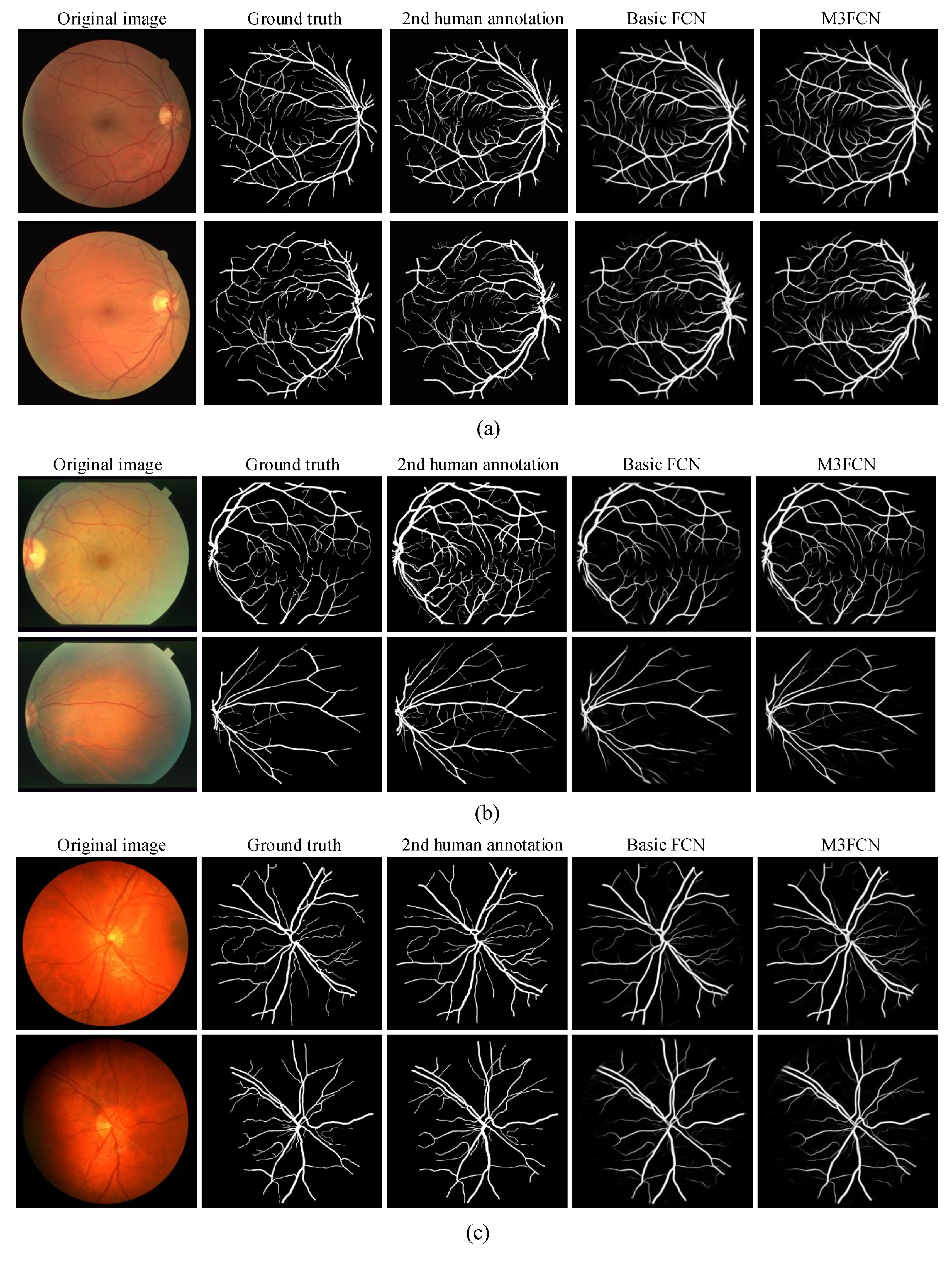
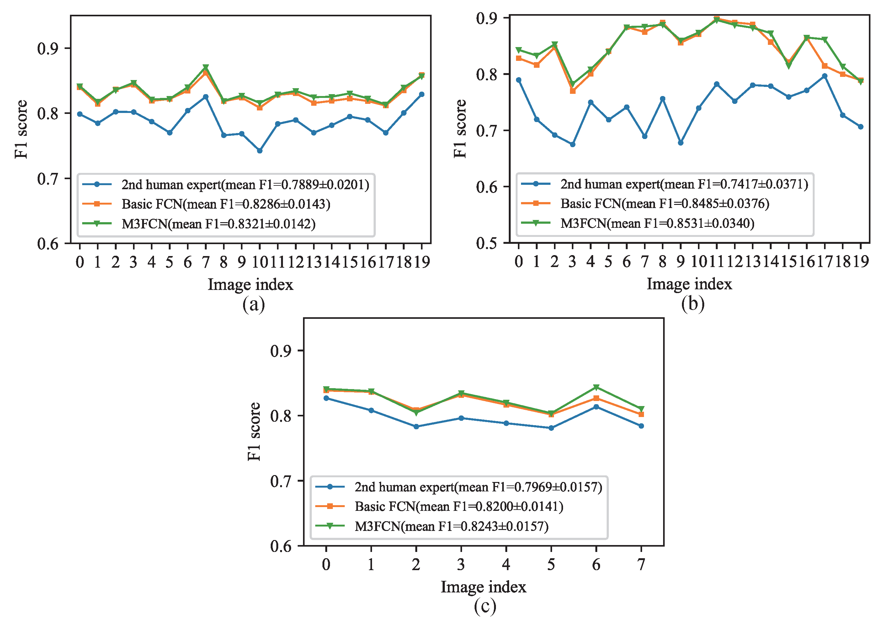
Visualizations of the segmented vessel probability map of M3FCN for all three datasets are shown in Figure 9. In Figure 10, we visualize the results of the F1 score for each test image in the DRIVE, STARE, and CHASE datasets to further observe the segmentation results. From the segmentation results, the M3FCN is better than the basic FCN and the 2nd human expert. It can be seen from the mean and standard deviation that the segmentation result of M3FCN is more accurate and stable than the results of basic FCN and second human expert segmentation. This indicates that the M3FCN is highly generalized, has a strong ability to extract and recognize features, and can well segment the blood vessels of various retinal images. Whether in healthy or diseased retinal images, M3FCN can maintain a relatively stable segmentation effect, which can overcome the impact of lesions well.
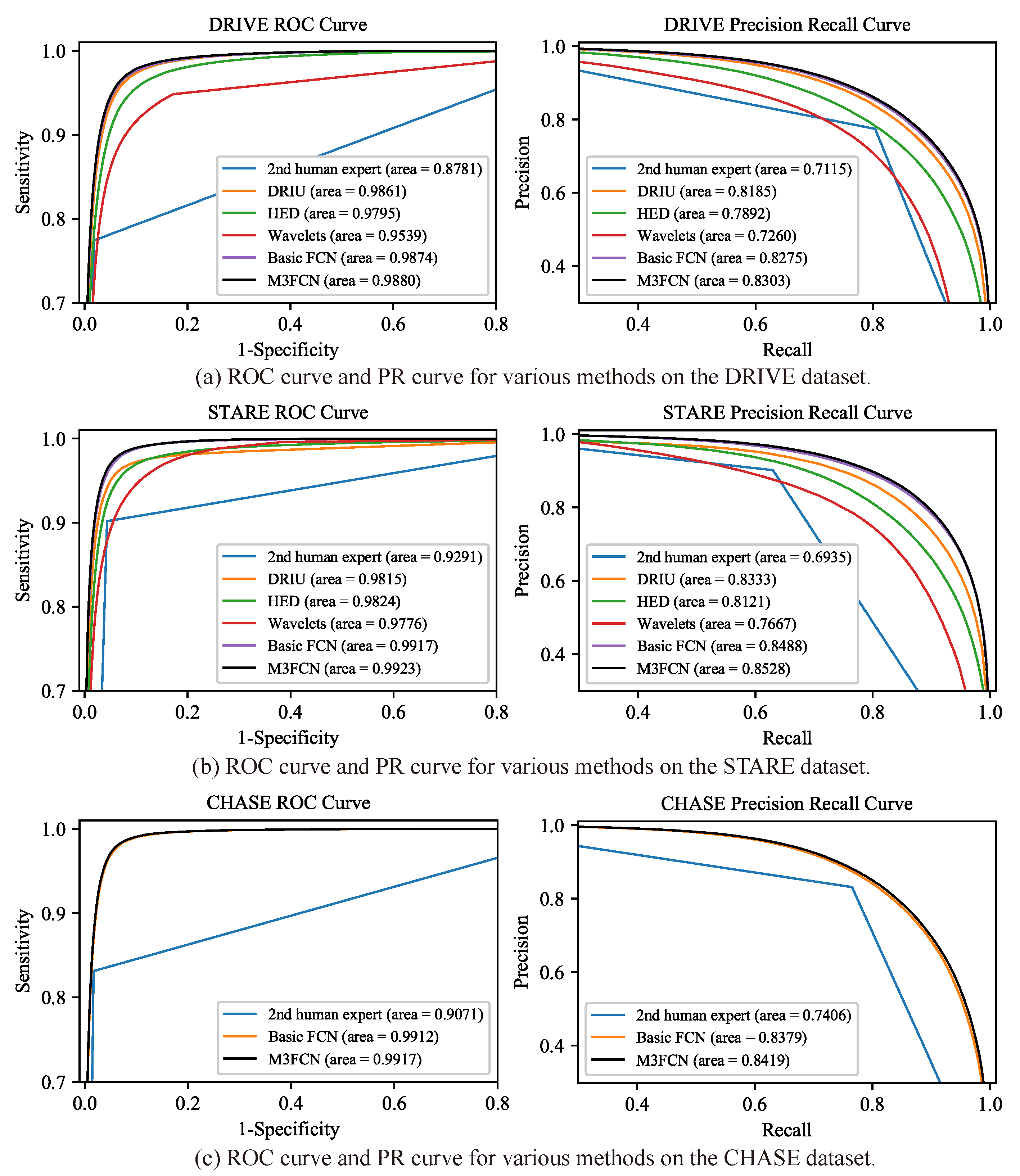
In Figure 11, the Receiver Operating Characteristic (ROC) curve and Precision Recall (PR) curve are computed and visualized and compared with other several state-of-the-art methods such as DRIU [40], Wavelet [53], HED [54]. The ROC curve gives information between the false positive pixel and the true positive pixel in the form of a fraction based on the threshold change on the probability map. The PR curve can better reflect the true performance of the classification when the ratio of positive and negative samples is large. The difference from the upper left convex of the ROC curve is that the PR curve is the upper right convex effect. The ROC and PR curve area on the M3FCN is 0.19% and 1.18% higher than DRIU [40], respectively. We also visualized the curve of the 2nd human expert segmentation results, and the ROC and PR curve area were 0.8781 and 0.7115, respectively. The results show that M3FCN can achieve better segmentation results than the 2nd human expert. On the STARE and CHASE datasets, we can get the same conclusions as to the DRIVE dataset. The M3FCN obtains the best performances on the DRIVE dataset (0.9880 A U C R O C , 0.8303 A U C P R ), the STARE dataset (0.9923 A U C R O C , 0.8528 A U C P R ) and the CHASE dataset (0.9917 A U C R O C , 0.8419 A U C P R ). It can be observed that the curve of the proposed methods is increasing at the true positive rate that indicates better performance of the proposed method than all other existing methods. Compared with other methods, M3FCN can extract deeper representation features, better segment background information and fine vascular information.

5. Conclusions

In this paper, we have devised a novel automatic segmentation framework for retinal vessels. It is an end-to-end deep learning framework that has been improved from data preprocessing, data augmentation, and network architecture. Firstly, we explored the performance changes brought by various preprocessing methods and proposed a four-step preprocessing method to improve network performance. Secondly, we proposed a dynamic extraction patch strategy and Random Crop and Fill (RCF) data augmentation method to train the proposed M3FCN network. Finally, from the retinal image to the segmented image, it goes through the following steps: (1) preprocessing the retinal image according to the proposed four methods: grayscale, normalization, CHASE and gamma correction; (2) overlapping the retinal image to obtain patches, and inputting it into the trained M3FCN to obtain patch segmentation results; and (3) the patch segmentation results are reconstructed into the final segmentation image by the overlap patch reconstruction algorithm. Our framework is trained and tested using public datasets DRIVE, STARE, and CHASE. The F1 score, Accuracy, Sensitivity, Specificity, and AUC were used as indicators to demonstrate that the proposed framework had better performance. The results of different indicators show that the M3FCN has achieved state-of-the-art results.
Multiple experimental results demonstrate that the M3FCN is highly generalized for multiple datasets, indicating its potential for practical applications in screening and diagnostic systems. It has also proven to be fast because it consists primarily of convolutional modules and is implemented using an efficient GPU. Based on our blood vessel segmentation results, symmetric and asymmetric patterns can be extracted from retinal images and applied to computer-aided diagnostic systems. In addition, future work will focus on combining other new methods and experimenting with more standard open datasets.

Author Contributions

Methodology, H.Z.; Software, H.Z.; Supervision, Y.J.; Validation, N.T.; Writing—original draft, H.Z.; Writing—review and editing, H.Z. and L.C.

Funding

This work was supported by the National Natural Science Foundation of China (61962054), the 2016 Gansu Provincial Science and Technology Plan Funded Natural Science Fund Project (1606RJZA047), the 2012 Gansu Provincial University Basic Research Business Expenses Special Fund Project, the Gansu Provincial University Graduate Tutor Project (1201-16), and the third phase of the Northwest Normal University knowledge and innovation engineering research backbone project (nwnu-kjcxgc-03-67).

Conflicts of Interest

The authors declare no conflict of interest. The funders had no role in the design of the study; in the collection, analyses, or interpretation of data; in the writing of the manuscript, or in the decision to publish the results.

References

  1. Soomro, T.A.; Khan, T.M.; Khan, M.A.; Gao, J.; Paul, M.; Zheng, L. Impact of ICA-based image enhancement technique on retinal blood vessels segmentation. IEEE Access 2018, 6, 3524–3538. [Google Scholar] [CrossRef]
  2. Dharmawan, D.A.; Li, D.; Ng, B.P.; Rahardja, S. A New Hybrid Algorithm for Retinal Vessels Segmentation on Fundus Images. IEEE Access 2019, 7, 41885–41896. [Google Scholar] [CrossRef]
  3. Hoover, A.; Kouznetsova, V.; Goldbaum, M. Locating blood vessels in retinal images by piecewise threshold probing of a matched filter response. IEEE Trans. Med. Imaging 2000, 19, 203–210. [Google Scholar] [CrossRef] [PubMed]
  4. Oliveira, W.S.; Teixeira, J.V.; Ren, T.I.; Cavalcanti, G.D.; Sijbers, J. Unsupervised retinal vessel segmentation using combined filters. PLoS ONE 2016, 11, e0149943. [Google Scholar] [CrossRef] [PubMed]
  5. Zardadi, M.; Mehrshad, N.; Razavi, S.M. Unsupervised Segmentation of Retinal Blood Vessels Using the Human Visual System Line Detection Model. 2016. Available online: https://pdfs.semanticscholar.org/10e1/a203cfdfe9d95e8d5e1b6fb23df03093de40.pdf (accessed on 26 August 2019).
  6. Fraz, M.M.; Barman, S.A.; Remagnino, P.; Hoppe, A.; Basit, A.; Uyyanonvara, B.; Rudnicka, A.R.; Owen, C.G. An approach to localize the retinal blood vessels using bit planes and centerline detection. Comput. Methods Prog. Biomed. 2012, 108, 600–616. [Google Scholar] [CrossRef] [PubMed]
  7. Hassan, G.; El-Bendary, N.; Hassanien, A.E.; Fahmy, A.; Snasel, V.; Shoeb, A.M. Retinal blood vessel segmentation approach based on mathematical morphology. Procedia Comput. Sci. 2015, 65, 612–622. [Google Scholar] [CrossRef]
  8. Liu, I.; Sun, Y. Recursive tracking of vascular networks in angiograms based on the detection-deletion scheme. IEEE Trans. Med. Imaging 1993, 12, 334–341. [Google Scholar] [CrossRef] [PubMed]
  9. Yin, Y.; Adel, M.; Bourennane, S. Retinal vessel segmentation using a probabilistic tracking method. Pattern Recognit. 2012, 45, 1235–1244. [Google Scholar] [CrossRef]
  10. Staal, J.; Abràmoff, M.D.; Niemeijer, M.; Viergever, M.A.; Van Ginneken, B. Ridge-based vessel segmentation in color images of the retina. IEEE Transact. Med. Imaging 2004, 23, 501–509. [Google Scholar] [CrossRef]
  11. You, X.; Peng, Q.; Yuan, Y.; Cheung, Y.M.; Lei, J. Segmentation of retinal blood vessels using the radial projection and semi-supervised approach. Pattern Recognit. 2011, 44, 2314–2324. [Google Scholar] [CrossRef]
  12. Tan, J.H.; Fujita, H.; Sivaprasad, S.; Bhandary, S.V.; Rao, A.K.; Chua, K.C.; Acharya, U.R. Automated segmentation of exudates, haemorrhages, microaneurysms using single convolutional neural network. Inf. Sci. 2017, 420, 66–76. [Google Scholar] [CrossRef]
  13. Aslani, S.; Sarnel, H. A new supervised retinal vessel segmentation method based on robust hybrid features. Biomed. Signal Process. Control 2016, 30, 1–12. [Google Scholar] [CrossRef]
  14. Fraz, M.M.; Remagnino, P.; Hoppe, A.; Uyyanonvara, B.; Rudnicka, A.R.; Owen, C.G.; Barman, S.A. An ensemble classification-based approach applied to retinal blood vessel segmentation. IEEE Trans. Biomed. Eng. 2012, 59, 2538–2548. [Google Scholar] [CrossRef] [PubMed]
  15. Fu, H.; Xu, Y.; Wong, D.W.K.; Liu, J. Retinal vessel segmentation via deep learning network and fully-connected conditional random fields. In Proceedings of the 2016 IEEE 13th International Symposium on Biomedical Imaging (ISBI), Prague, Czech Republic, 13–16 April 2016; pp. 698–701. [Google Scholar]
  16. Mo, J.; Zhang, L. Multi-level deep supervised networks for retinal vessel segmentation. Int. J. Comput. Assisted Radiol. Surg. 2017, 12, 2181–2193. [Google Scholar] [CrossRef] [PubMed]
  17. Lin, Y.; Zhang, H.; Hu, G. Automatic Retinal Vessel Segmentation via Deeply Supervised and Smoothly Regularized Network. IEEE Access 2018, 7, 57717–57724. [Google Scholar] [CrossRef]
  18. Owen, C.G.; Rudnicka, A.R.; Mullen, R.; Barman, S.A.; Monekosso, D.; Whincup, P.H.; Ng, J.; Paterson, C. Measuring retinal vessel tortuosity in 10-year-old children: Validation of the computer-assisted image analysis of the retina (CAIAR) program. Investig. Ophthalmol. Visual Sci. 2009, 50, 2004–2010. [Google Scholar] [CrossRef]
  19. Jin, Q.; Meng, Z.; Pham, T.D.; Chen, Q.; Wei, L.; Su, R. DUNet: A deformable network for retinal vessel segmentation. Knowl.-Based Syst. 2019, 178, 149–162. [Google Scholar] [CrossRef] [Green Version]
  20. Soares, J.V.; Leandro, J.J.; Cesar, R.M.; Jelinek, H.F.; Cree, M.J. Retinal vessel segmentation using the 2-D Gabor wavelet and supervised classification. IEEE Trans. Med. Imaging 2006, 25, 1214–1222. [Google Scholar] [CrossRef] [Green Version]
  21. Zhuang, J. LadderNet: Multi-path networks based on U-Net for medical image segmentation. arXiv 2018, arXiv:1810.07810. [Google Scholar]
  22. Payette, B. Color Space Converter: R’G’B’to Y’CbCr; Xilinx, XAPP637 (v1. 0); Xilinx: San Jose, CA, USA, 2002. [Google Scholar]
  23. Ioffe, S.; Szegedy, C. Batch normalization: Accelerating deep network training by reducing internal covariate shift. arXiv 2015, arXiv:1502.03167. [Google Scholar]
  24. Jain, A.; Nandakumar, K.; Ross, A. Score normalization in multimodal biometric systems. Pattern Recognit. 2005, 38, 2270–2285. [Google Scholar] [CrossRef]
  25. Pizer, S.M.; Amburn, E.P.; Austin, J.D.; Cromartie, R.; Geselowitz, A.; Greer, T.; ter Haar Romeny, B.; Zimmerman, J.B.; Zuiderveld, K. Adaptive histogram equalization and its variations. Comput. Vis. Graph. Image Process. 1987, 39, 355–368. [Google Scholar] [CrossRef]
  26. Bradski, G.; Kaehler, A. Learning OpenCV: Computer Vision with the OpenCV Library; O’Reilly Media, Inc.: Newton, MA, USA, 2008. [Google Scholar]
  27. Oliveira, A.; Pereira, S.; Silva, C.A. Retinal vessel segmentation based on fully convolutional neural networks. Expert Syst. Appl. 2018, 112, 229–242. [Google Scholar] [CrossRef]
  28. Kingma, D.P.; Ba, J. Adam: A method for stochastic optimization. arXiv 2014, arXiv:1412.6980. [Google Scholar]
  29. He, K.; Zhang, X.; Ren, S.; Sun, J. Deep residual learning for image recognition. In Proceedings of the IEEE Conference on Computer Vision and Pattern Recognition, Las Vegas, NV, USA, 27–30 June 2016; pp. 770–778. [Google Scholar]
  30. Long, J.; Shelhamer, E.; Darrell, T. Fully convolutional networks for semantic segmentation. In Proceedings of the IEEE Conference on Computer Vision and Pattern Recognition, Boston, MA, USA, 7–12 June 2015; pp. 3431–3440. [Google Scholar]
  31. Xu, B.; Wang, N.; Chen, T.; Li, M. Empirical evaluation of rectified activations in convolutional network. arXiv 2015, arXiv:1505.00853. [Google Scholar]
  32. Nair, V.; Hinton, G.E. Rectified linear units improve restricted boltzmann machines. In Proceedings of the 27th International Conference on Machine Learning (ICML-10), Haifa, Israel, 21–24 June 2010; pp. 807–814. [Google Scholar]
  33. He, K.; Zhang, X.; Ren, S.; Sun, J. Delving deep into rectifiers: Surpassing human-level performance on imagenet classification. In Proceedings of the IEEE International Conference on Computer Vision, Washington, DC, USA, 7–13 December 2015; pp. 1026–1034. [Google Scholar]
  34. Paszke, A.; Gross, S.; Chintala, S.; Chanan, G.; Yang, E.; DeVito, Z.; Lin, Z.; Desmaison, A.; Antiga, L.; Lerer, A. Automatic differentiation in pytorch. In Proceedings of the 31st Conference on Neural Information Processing Systems (NIPS 2017), Long Beach, CA, USA, 4–9 December 2017. [Google Scholar]
  35. Lam, B.S.; Gao, Y.; Liew, A.W.C. General retinal vessel segmentation using regularization-based multiconcavity modeling. IEEE Trans. Med. Imaging 2010, 29, 1369–1381. [Google Scholar] [CrossRef] [PubMed]
  36. Fraz, M.M.; Remagnino, P.; Hoppe, A.; Uyyanonvara, B.; Rudnicka, A.R.; Owen, C.G.; Barman, S.A. Blood vessel segmentation methodologies in retinal images—A survey. Comput. Methods Programs Biomed. 2012, 108, 407–433. [Google Scholar] [CrossRef] [PubMed]
  37. Azzopardi, G.; Strisciuglio, N.; Vento, M.; Petkov, N. Trainable COSFIRE filters for vessel delineation with application to retinal images. Med. Image Anal. 2015, 19, 46–57. [Google Scholar] [CrossRef] [PubMed] [Green Version]
  38. Ronneberger, O.; Fischer, P.; Brox, T. U-net: Convolutional networks for biomedical image segmentation. In Proceedings of the International Conference on Medical Image Computing and Computer-Assisted Intervention, Springer, Munich, Germany, 5–9 October 2015; pp. 234–241. [Google Scholar]
  39. Liskowski, P.; Krawiec, K. Segmenting retinal blood vessels with deep neural networks. IEEE Trans. Med. Imaging 2016, 35, 2369–2380. [Google Scholar] [CrossRef] [PubMed]
  40. Maninis, K.K.; Pont-Tuset, J.; Arbeláez, P.; Van Gool, L. Deep retinal image understanding. In Proceedings of the International Conference on Medical Image Computing and Computer-Assisted Intervention, Athens, Greece, 17–21 October 2016; pp. 140–148. [Google Scholar]
  41. Orlando, J.I.; Prokofyeva, E.; Blaschko, M.B. A discriminatively trained fully connected conditional random field model for blood vessel segmentation in fundus images. IEEE Trans. Biomed. Eng. 2016, 64, 16–27. [Google Scholar] [CrossRef] [PubMed]
  42. Dasgupta, A.; Singh, S. A fully convolutional neural network based structured prediction approach towards the retinal vessel segmentation. In Proceedings of the 2017 IEEE 14th International Symposium on Biomedical Imaging (ISBI 2017), Melbourne, Australia, 18–21 April 2017; pp. 248–251. [Google Scholar]
  43. Zhang, J.; Chen, Y.; Bekkers, E.; Wang, M.; Dashtbozorg, B.; ter Haar Romeny, B.M. Retinal vessel delineation using a brain-inspired wavelet transform and random forest. Pattern Recognit. 2017, 69, 107–123. [Google Scholar] [CrossRef]
  44. Xia, H.; Jiang, F.; Deng, S.; Xin, J.; Doss, R. Mapping Functions Driven Robust Retinal Vessel Segmentation via Training Patches. IEEE Access 2018, 6, 61973–61982. [Google Scholar] [CrossRef]
  45. Alom, M.Z.; Hasan, M.; Yakopcic, C.; Taha, T.M.; Asari, V.K. Recurrent residual convolutional neural network based on u-net (R2U-net) for medical image segmentation. arXiv 2018, arXiv:1802.06955. [Google Scholar]
  46. Lu, J.; Xu, Y.; Chen, M.; Luo, Y. A Coarse-to-Fine Fully Convolutional Neural Network for Fundus Vessel Segmentation. Symmetry 2018, 10, 607. [Google Scholar] [CrossRef]
  47. Li, Q.; Feng, B.; Xie, L.; Liang, P.; Zhang, H.; Wang, T. A cross-modality learning approach for vessel segmentation in retinal images. IEEE Trans. Med. Imaging 2015, 35, 109–118. [Google Scholar] [CrossRef] [PubMed]
  48. Son, J.; Park, S.J.; Jung, K.H. Retinal vessel segmentation in fundoscopic images with generative adversarial networks. arXiv 2017, arXiv:1706.09318. [Google Scholar]
  49. Li, R.; Li, M.; Li, J. Connection sensitive attention U-NET for accurate retinal vessel segmentation. arXiv 2019, arXiv:1903.05558. [Google Scholar]
  50. Zhang, B.; Huang, S.; Hu, S. Multi-scale neural networks for retinal blood vessels segmentation. arXiv 2018, arXiv:1804.04206. [Google Scholar]
  51. Yan, Z.; Yang, X.; Cheng, K.T.T. A three-stage deep learning model for accurate retinal vessel segmentation. IEEE J. Biomed. Health Inform. 2018, 23, 1427–1436. [Google Scholar] [CrossRef]
  52. Chen, C.; Bai, W.; Davies, R.H.; Bhuva, A.N.; Manisty, C.; Moon, J.C.; Aung, N.; Lee, A.M.; Sanghvi, M.M.; Fung, K.; et al. Improving the generalizability of convolutional neural network-based segmentation on CMR images. arXiv 2019, arXiv:1907.01268. [Google Scholar]
  53. Dua, S.; Acharya, U.R.; Chowriappa, P.; Sree, S.V. Wavelet-based energy features for glaucomatous image classification. IEEE Trans. Inf. Technol. Biomed. 2011, 16, 80–87. [Google Scholar] [CrossRef] [PubMed]
  54. Xie, S.; Tu, Z. Holistically-nested edge detection. In Proceedings of the IEEE International Conference on Computer Vision, Santiago, Chile, 7–13 December 2015; pp. 1395–1403. [Google Scholar]
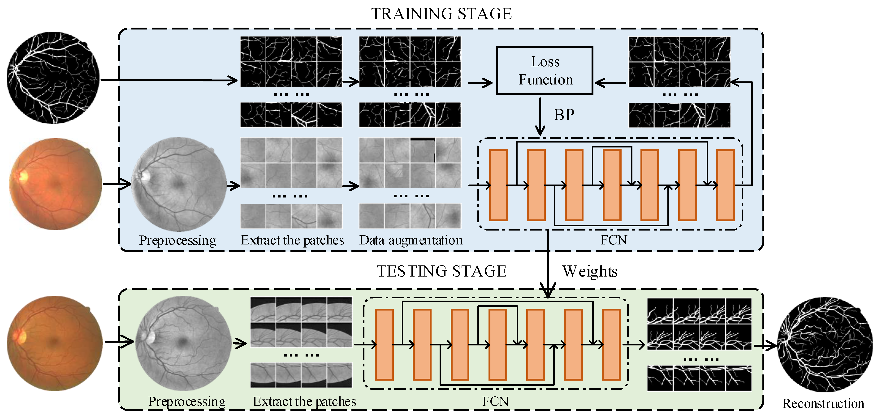
Figure 1. Overview of the proposed framework.
Symmetry 11 01112 g001
Figure 2. Examples of color images (first row) and labels (second row) from different datasets.
Symmetry 11 01112 g002
Figure 3. (a) is the original image. (bd) are visualizations of red, green, and blue channels, respectively. Results of each preprocessing strategy: (e) grayscale; (f) data normalization; (g) CLAHE; (h) Gamma correction.
Symmetry 11 01112 g003
Figure 4. Visualization of the Random Crop and Fill (RCF) method. (a) cropping; (b) RCF-R; (c) RCF-0; (d) RCF-A.
Symmetry 11 01112 g004
Figure 5. The basic FCN architecture.
Symmetry 11 01112 g005
Figure 6. The M3FCN architecture.
Symmetry 11 01112 g006
Figure 7. Test results under different hyper-parameters on DRIVE using M3FCN.
Symmetry 11 01112 g007
Figure 8. Visualization of F1 scores for different methods.
Symmetry 11 01112 g008
Figure 9. Visualization of the random samples results for each test dataset: (a) DRIVE; (b) STARE; (c) CHASE.
Symmetry 11 01112 g009
Figure 10. Visualize the F1 score and comparison of the image segmentation results for each image in the test dataset: (a) DRIVE; (b) STARE; (c) CHASE.
Symmetry 11 01112 g010
Figure 11. Visualize the ROC curves and the PR curves.
Symmetry 11 01112 g011
Table 1. Test results with different image preprocessing on DRIVE based on M3FCN.
No.GrayscaleData NormalizationCLAHEGamma CorrectionF1AccuracySensitivitySpecificityAUC
0 0.80480.95460.73500.98660.9771
1 0.81990.96920.80000.98550.9831
2 0.82290.96970.80430.98550.9852
3 0.82840.97020.82150.98450.9871
4 0.81680.96830.80810.98360.9839
5 0.82990.96990.83760.98260.9873
6 0.81730.96780.82340.98160.9840
7 0.82920.97040.82060.98480.9873
80.83210.97060.83250.98380.9880
Table 2. Test results under different hyper-parameters on DRIVE using M3FCN.
MethodF1AccuracySensitivitySpecificityAUC
-0.82880.97030.81980.98480.9870
RCF-00.82990.97020.82980.98370.9873
RCF-R0.82940.97020.82690.98400.9873
RCF-A0.83210.97060.83250.98380.9880
Table 3. Test results with data augmentation and RCF-A on DRIVE based on M3FCN. DA: Data augmentation.
MethodF1AccuracySensitivitySpecificityAUC
0.82420.96970.81110.98490.9861
DA0.82880.97030.81980.98480.9870
RCF-A0.82550.96890.83920.98140.9866
DA + RCF-A0.83210.97060.83250.98380.9880
Table 4. Test results with different improved FCN on DRIVE.
Model NameF1AccuracySensitivitySpecificityAUC
Basic FCN0.82860.97030.81960.98480.9870
Muiti-scale FCN0.82900.97070.81150.98600.9873
Multi-path FCN0.82870.97060.81180.98580.9871
Multi-output fusion FCN0.82930.97050.81920.98500.9870
Muiti-scale, multi-path FCN0.82950.97030.82590.98410.9870
Muiti-scale, multi-output fusion FCN0.82860.97080.80630.98660.9871
Muiti-path, multi-output fusion FCN0.83040.97010.83700.98280.9873
M3FCN0.83210.97060.83250.98380.9880
Table 5. Comparison of proposed methods with other methods in the DRIVE dataset.
MethodsYearF1AccuracySensitivitySpecificityAUC
2nd human expert-0.78890.96370.77430.98190.8781
Lam et al. [35]2010-0.9472--0.9614
You et al. [11]2011-0.94340.74100.9751-
Fraz et al. [36]2012-0.94300.71520.9759-
Azzopardi et al. [37]2015-0.94420.76550.97040.9614
Ronneberger et al. [38]20150.81420.95310.75370.98200.9755
Liskowsk et al. [39]2016-0.94950.77630.97680.9720
Maninis et al. [40]20160.82100.95410.82610.91150.9861
Orlando et al. [41]20170.7857-0.78970.9684-
Dasgupta et al. [42]20170.80740.95330.76910.98010.9744
Zhang et al. [43]20170.79530.94660.78610.97120.9703
Xia et al. [44]2018-0.95400.77400.9800-
Alom et al. [45]20180.81710.95560.77920.98130.9784
Zhuang et al. [21]20180.82020.95610.78560.98100.9793
Lu et al. [46]2018-0.96340.79410.98700.9787
Oliveira et al. [27]2018-0.95760.80390.98040.9821
Jin et al. [19]20190.82370.95660.79630.98000.9802
Basic FCN (ours)20190.82860.97030.81970.98480.9874
M3FCN (ours)20190.83210.97060.83250.98380.9880
Table 6. Comparison of proposed methods with other methods in the STARE dataset.
MethodsYearF1AccuracySensitivitySpecificityAUC
2nd human expert-0.74170.95220.90170.95640.9291
Lam et al. [35]2010-0.9567--0.9739
Fraz et al. [36]2012-0.94420.73110.9680-
Azzopardi et al. [37]2015-0.95630.77160.97010.9497
Li et al. [47]2015-0.96280.77260.98440.9879
Ronneberger et al. [38]20150.83730.96900.82700.98420.9898
Liskowsk et al. [39]2016-0.95660.78670.97540.9785
Maninis et al. [40]20160.82100.95410.82610.91150.9861
Orlando et al. [41]20170.7701-0.76800.9738-
Son et al. [48]20170.83530.96570.8350-0.9777
Zhang et al. [43]20170.78150.95470.78820.97290.9740
Oliveira et al. [27]2018-0.96940.83150.98580.9905
Xia et al. [44]2018-0.95300.76700.9770-
Lu et al. [46]2018-0.96280.80900.97700.9801
Li et al. [49]20190.84350.96730.8465-0.9834
Jin et al. [19]20190.81430.96410.75950.98780.9832
Basic FCN (ours)20190.84850.97730.83690.98880.9917
M3FCN (ours)20190.85310.97770.85220.98800.9923
Table 7. Comparison of proposed methods with other methods in the CHASE dataset.
MethodsYearF1AccuracySensitivitySpecificityAUC
2nd human expert-0.79690.97330.83130.98290.9071
Lam et al. [35]2015-0.93870.75850.95870.9487
Li et al. [47]2015-0.95810.75070.97930.9793
Ronneberger et al. [38]20150.77830.95780.82880.97010.9772
Liskowsk et al. [39]2016-0.95660.78670.97540.9785
Zhang et al. [43]20170.75810.95020.76440.97160.9706
Zhang et al. [50]2018-0.96620.77420.98760.9865
Alom et al. [45]20180.79280.96340.77560.98200.9815
Zhuang et al. [21]20180.80310.96560.79780.98180.9839
Lu et al. [46]2018-0.96640.75710.98230.9752
Jin et al. [19]20190.78830.96100.81550.97520.9804
Basic FCN (ours)20190.82000.97700.83230.98670.9912
M3FCN (ours)20190.82430.97730.84530.98620.9917
Table 8. Comparison of experimental results: training models using the STARE dataset, then testing on the DRIVE dataset.
MethodYearF1AccuracySensitivitySpecificityAUC
Fraz et al. [14]2012-0.94560.72420.97920.9697
Li et al. [47]2015-0.94860.72730.98100.9677
Yan et al. [51]2018-0.94440.70140.98020.9568
Jin et al. [19]2019-0.94810.65050.99140.9718
Basic FCN(ours)20190.76750.96460.66630.99330.9780
M3FCN (ours)20190.78450.96650.69500.99260.9820
Table 9. Comparison of experimental results: training models using the DRIVE dataset, then testing on the STARE dataset.
MethodYearF1AccuracySensitivitySpecificityAUC
Fraz et al. [14]2012-0.94950.70100.97700.9660
Li et al. [47]2015-0.95450.70270.98280.9671
Yan et al. [51]2018-0.95800.73190.98400.9678
Jin et al. [19]2019-0.94450.84190.95630.9690
Basic FCN (ours)20190.77550.96330.83320.97400.9790
M3FCN (ours)20190.78760.96470.86040.97330.9826