Article

Visual Meterstick: Preceding Vehicle Ranging Using Monocular Vision Based on the Fitting Method

1
Beijing Key Laboratory of Information Service Engineering, Beijing Union University, No.97 Beisihuan East Road, Chao Yang District, Beijing 100101, China
2
School of Mechanical Electronic & Information Engineering, China University of Mining & Technology, Beijing 100083, China
*
Author to whom correspondence should be addressed.
Symmetry 2019, 11(9), 1081; https://doi.org/10.3390/sym11091081
Submission received: 10 August 2019 / Revised: 25 August 2019 / Accepted: 26 August 2019 / Published: 28 August 2019

Abstract

:
The gradual application of deep learning in the field of computer vision and image processing has made great breakthroughs. Applications such as object detection, recognition and image semantic segmentation have been improved. In this study, to measure the distance of the vehicle ahead, a preceding vehicle ranging system based on fitting method was designed. First obtaining an accurate bounding box frame in the vehicle detection, the Mask R-CNN (region-convolutional neural networks) algorithm was improved and tested in the BDD100K (Berkeley deep derive) asymmetry dataset. This method can shorten vehicle detection time by 33% without reducing the accuracy. Then, according to the pixel value of the bounding box in the image, the fitting method was applied to the vehicle monocular camera for ranging. Experimental results demonstrate that the method can measure the distance of the preceding vehicle effectively, with a ranging error of less than 10%. The accuracy of the measurement results meets the requirements of collision warning for safe driving.

Graphical Abstract

1. Introduction

As a basic technology in the field of computer vision, visual ranging occupies an important position. It is widely used in the research of visual navigation, machine vision positioning, target tracking, etc., especially in human–computer interaction systems [1]. Monocular vision ranging refers to the use of a digital camera to capture a single image to measure distance. The procedure of obtaining the distance of the preceding vehicle with visual ranging mainly includes the following two steps: First, object detection, finding the object (the preceding vehicle) to be detected in the image. Second, object ranging, using the real world and the target position in the picture. The corresponding relationship determines the true distance between the target object and the camera. The accuracy of target recognition has a direct impact on object ranging. For this purpose, this paper researches the method of monocular vision measurement of vehicle distance.
Front vehicle detection is one of the research contents of computer vision for identifying and locating vehicles in images or videos. In the field of ITS (intelligent transport system) and IV (intelligent video) research at home and abroad, many algorithms and implementation methods for vehicle detection have been proposed. Researchers have made some progress in applied machine learning for vehicle detection [2], but the current vehicle detection research still faces the following major problems: The complex and diverse actual road conditions, the various types, multiple colors and different sizes of vehicles and the insufficiency of the model training data [3]. Some vehicles have large area occlusion problems. This increases the matching difficulty based on the vehicle detection model to some extent. In addition, smart driving is especially demanding for real-time SVM (support vector machine) or neural networks. The machine-based learning method cannot meet the safety requirements of intelligent driving in terms of vehicle detection time [4]. Constructing a deep network through deep learning to extract vehicle target features is currently a hot research topic of vehicle detection technology [5]. In order to solve these problems, this paper proposes a method based on the improved Mask R-CNN, which removes the RoIAlign layer of the Mask R-CNN, and improves the speed of training and detection without reducing the detection accuracy. The experimental results show that, compared with the existing Mask R-CNN vehicle detection method, the performance of the method is improved, which provides a more general and simple solution for the problem of vehicle detection ahead.
At present, the focus of research in vehicle ranging technology is monocular ranging and multi-target ranging, and binocular ranging is more commonly known. In contrast, binocular vision ranging is more accurate, but it still has some problems that limit its application. Since binocular ranging requires precise matching, and the matching process is time consuming, it is not negligible for the real-time impact of the visual navigation system [6]. In addition, binocular measurement has high requirements for some special constraints, such as camera resolution, imaging quality, distance between the left and right camera optical axes, camera focal length, etc., which are very strict in the quality and installation of the camera and measurement platform standards. On the other hand, the monocular depth extraction method, with only one camera and less constraint requirements than binocular ranging, has the advantages of higher usability, simple operation and low cost. Thus, monocular vision ranging conforms more closely to the experimental requirements. First, the distance model is established by the transformation of two-dimensional images and three-dimensional space. Then, after obtaining the value of the bounding box of the vehicle through the first step, the internal and external parameters of the camera are based on the bounding box center. The coordinate value of the point is measured by the fitting method. Even if the abscissa and the ordinate of the pixel in the image are fitted to the actual distance to calculate a certain functional relationship, the actual distance of the obstacle is calculated. Finally, the experimental results are used to analyze whether the error is within the allowable range of the experiment.

2. Related Work

2.1. Vehicle Detection Improved Method

2.1.1. RoIAlign Layer

Instance segmentation is challenging because it requires the correct detection of all objects in an image while precisely segmenting each instance. It therefore combines elements from the classical computer vision tasks of object detection where the goal is to classify individual objects and localize each using a bounding box and semantic segmentation and to classify each pixel into a fixed set of categories without differentiating object instances [7]. Given this, one might expect that a complex method is required to achieve good results. Mask R-CNN extends Faster R-CNN [8] by adding a branch for predicting segmentation masks on each Region of Interest (RoI) in parallel with the existing branch for classification and bounding box regression (Figure 1). The mask branch is a small FCN (feature pyramid networks) applied to each RoI, predicting a segmentation mask in a pixel-to-pixel manner [9].
RoIPool is the standard operation for extracting feature maps from each RoI. RoIPool first quantifies the RoI represented by floating-point numbers to the granularity matched with the feature graph, then divides the quantized RoI into blocks, and finally summarizes the eigenvalues of the regions covered by each block. Quantization operation has little effect on classified images, but it has a larger effect on fine pixel-level segmentation images [10]. To solve these problems, a RoIAlign layer is proposed, which mainly eliminates the rough quantization of RoIPool and aligns the extracted features and pixels accurately. Four regular positions in each RoI block are selected, and the precise values of each position are calculated by bilinear difference. The results are then summarized [11].

2.1.2. Improved Mask R-CNN Structure and Training Process

The Mask-RCNN framework or Faster-RCNN framework can be said to add a fully connected partitioned subnet after the basic feature network. Mask R-CNN is a two-stage framework. The first stage scans the image and generates proposals. The second stage classifies proposals and generates boundary boxes and masks. The method proposed in this paper is to annotate the RoIAlign layer and not to train the case segmentation. After FPN generates the suggestion window, it maps the suggestion window to the last convolution feature map of CNN. Then it directly uses full connection classification, border and mask to regress. The overall process is shown in Figure 2.

2.2. Experimental Results and Analysis

2.2.1. Experimental Environment

In the field of machine learning and computer vision for the development of deep learning, most are constructed with TensorFlow as the main learning framework. TensorFlow is a framework for open source software. TensorFlow has a multi-tiered architecture that can be deployed on a variety of servers, PC terminals and web pages and supports GPU (graphics processing unit) and TPU (tensor processing unit) high performance numerical computing. Therefore, this article still uses TensorFlow to build a deep learning framework. The operating system is Ubuntu16.04, using Python3.5 as the main compilation environment; the main graphics card model used in computer hardware is TITAN V; the CPU is I9 7900X.

2.2.2. Datasets

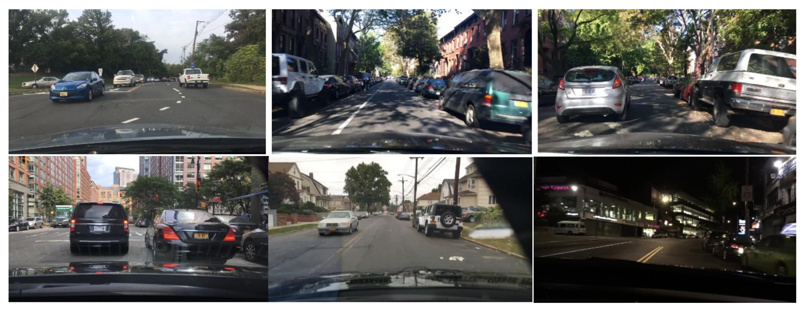
Berkeley University, BDD100K. The BDD100K asymmetry dataset contains 100,000 segments of HD video. Each video is about 40 s, 720 p, 30 fps [12]. The key frame is sampled in the 10th second of each video to get 100,000 images (image size: 1280 × 720). There are 10 categories of labels in the dataset: Bus, light, sign, person, bike, truck, motor, car, train and rider. There are about 1.84 million calibration frames in total, and the number of different types of targets is shown in Figure 3.
This article selects 99,292 images containing vehicle tags, as shown in Figure 4.

2.2.3. Evaluation Metrics

Under the same conditions, the three kinds of convolutional neural networks, Fast R-CNN, Faster R-CNN, and Mask R-CNN, are discussed in terms of the calibration frame precision and the processing time of a single image. The evaluation criteria are as shown in Equation (1):
M I o U = 1 k + 1 i = 0 k p i i j = 0 k p i j + j = 0 k p j i p i i
Mean intersection over union (MIoU), p i j , indicates that the true value is i, which is predicted as the number of j.
The experimental comparison results are listed in Table 1 and Table 2.
Table 1 can be used to obtain the ideal results of the calibration frame accuracy and average running time of the Mask R-CNN. Table 2 shows that the training time of the model can be reduced by 25% after deleting the RoIAlign layer. The test time was reduced by 33%. This paper has practical significance in solving the vehicle detection within a limited time.

3. Preceding Vehicle Ranging

There are three main methods of ranging based on machine vision: Binocular vision measurement, monocular vision measurement [13] and structured light vision measurement [14]. Due to the limitation and influence of the light source, the structured light is scarcely applied and fixed; the theoretical research of binocular vision ranging focuses on the matching of features [15,16]. The difficulty lies in the accuracy of feature point matching. It affects the efficiency and accuracy of measurement, while monocular vision has broad application prospects due to its fast calculation speed and simple structure. At the same time, object ranging based on monocular vision is widely used in the fields of driverless cars and autonomous mobile robots. It is extremely significant. It can accurately acquire spatial parameters such as distance, posture and orientation of the preceding object and is applied to driverless cars, navigation and path planning aspects.
There are three main ranging models based on monocular vision: Ranging models based on the principle of small hole imaging, ranging models based on sequence images and ranging models based on single-frame static images [17].
The monocular vision vehicle ranging method can be divided into the following four categories. The first is based on the imaging model method, and the literature [18] uses the vehicle width to measure the vehicle distance. This method requires the actual width of the known vehicle and the width of different vehicles. The width of different vehicles varies from 1.4 m to 2.6 m; if the actual width of the vehicle is unknown in advance, it will cause a large ranging error. The authors of [19] use the position of the vehicle in the image to measure the distance of the vehicle. This method needs to accurately obtain the position of the vehicle in the image, otherwise it will generate a large ranging error. The second is a method based on geometric relations.To achieve vehicle ranging, the literature [20] uses the geometric positional relationship of the vehicle in the imaging model to derive the correspondence between the image coordinate system and the world coordinate system. This type of method requires accurate measurement of the camera’s viewing angle and pitch angle, otherwise the accuracy of the range is greatly reduced, and it is difficult to accurately measure the pitch angle for a camera on a moving vehicle. The third is based on mathematical regression modeling. For example, the literature [21] uses the correspondence between different reference distances and their positions in the image to calculate the regression model to measure the distance. This method requires a large amount of up-front data acquisition, analysis and calculation of mathematical models. The fourth is based on machine learning methods, and the literature [22] proposes a forward vehicle detection method that combines machine learning with prior knowledge. Vehicle candidate regions are extracted by using MB–LBP (multiscale block–local binary pattern) and Adaboost [23], and the vehicle is false detected based on the horizontal edges and grayscale features in the candidate regions. In addition, based on the vehicle detection, the improved vehicle bottom shadow positioning method is used to obtain the accurate position of the vehicle, and the vehicle distance measurement is realized by the position information imaging model method.
In order to solve the problem of poor environmental adaptability and low robustness in vehicle detection, this paper proposes a method of combining the imaging model and data fitting. According to the vehicle bounding box frame detected by Mask R-CNN, the relationship between the position of the vehicle in the image and the actual distance is established, and the polynomial function is established to realize the vehicle ranging by the fitting method.

4. Results

4.1. Establishment of Monocular Vision Ranging Model

4.1.1. Coordinate System Conversion

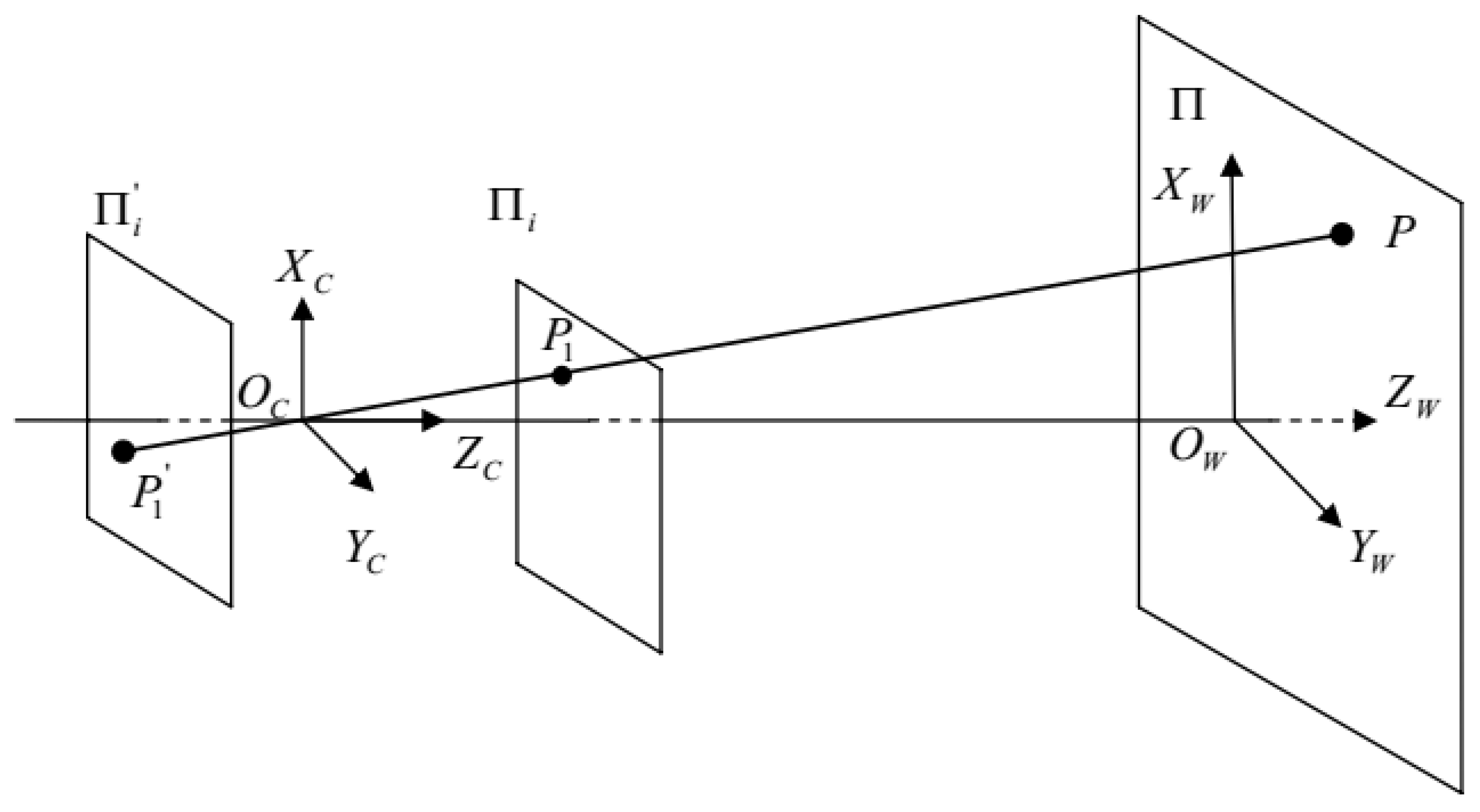
According to the camera mathematical model [24,25], the machine vision maps the scene projection in the three-dimensional world and coordinates to the pixel value of the two-dimensional gray matrix using the cooperative symbol fixed by the geometric dimension. The most common phenomenon is the pinhole camera model. The conversion process is shown in Figure 5 below.
(1) World coordinate to camera coordinate conversion.
Both the world point and the camera are in a three-dimensional coordinate system, and only a proper rotation and translation are required to convert specific virtual world coordinates to camera-centric camera coordinates. Take the linear camera model, the small hole imaging model, as an example [26,27], as shown in Figure 6. The arbitrary P-point world coordinates are X w , Y w , Z w ; the conversion relationship between world coordinates and camera coordinates can be obtained by the unit orthogonal rotation matrix R and the translation vector T.
X c Y c Z c = R X w Y w Z w + T
(2) Camera coordinate to plane coordinate conversion.
In Figure 6, O c is the optical center of the camera, which is the origin of the camera coordinate system. The Z c axis is parallel to the optical axis of the camera. The direction of each coordinate axis is as shown. In the camera coordinate system, assume that the coordinates of a point are P x , y , z . The projection point of point P on the imaging plane i is P 1 X 1 , Y 1 , Z 1 , f is the focal length of the camera and the formula for the conversion relationship is as follows.
x y = x 1 y 1 = x 1 f y z = y 1 z 1 = y 1 f
Conversion into a matrix is shown in Equation (4).
z x 1 y 1 1 = f 0 0 0 0 f 0 0 0 1 1 0 x y z 1
(3) Conversion from plane coordinates to pixel coordinates.
The pixel coordinate system is a two-dimensional coordinate, and the origin is freely selected. Assuming that the pixel coordinate origin is u 0 , v 0 , the image coordinates of the arbitrary coordinates (u, v) are:
u v 1 = s x 0 u 0 0 s y v 0 0 0 1 x y 1
In summary, the relationship between the conversion of the world coordinate system to the pixel coordinate system is as shown in Equation (6).
z c u v 1 = s x 0 u 0 0 s y v 0 0 0 1 * f 0 0 0 1 f 0 0 0 0 1 0 R T 0 1 X w Y w Z w 1
This is simplified as shown in Equation (7).
z c u v 1 = f x 0 u 0 0 0 f y v 0 0 0 0 1 0 R T 0 1 X w Y w Z w 1
Among them, f x , f y , u 0 and v 0 are the internal parameters of the camera, and R and T are external parameters, which are constrained by external conditions.

4.1.2. Data Regression Modeling

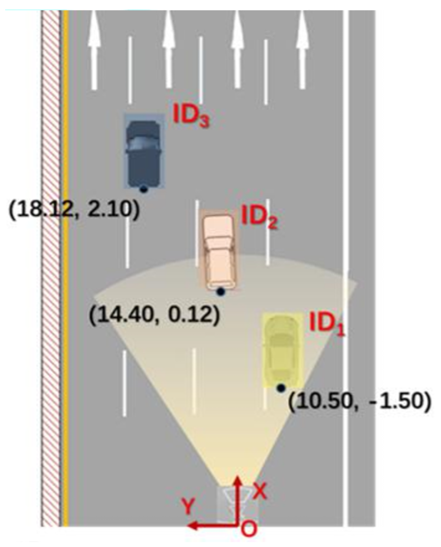
Literature [21] has proposed a monocular vision ranging method based on data regression modeling. The main idea is the reverse of “first modeling and then ranging” or “first ranging and re-modeling”. This method does not require any assumptions about the actual road scene to simplify the problem. Firstly, some distance sample points are obtained through calibration test, and the relationship between independent variables and dependent variables is studied. The mapping curve is drawn, and nonlinear regression is performed to establish a mathematical model. The obtained model is then used for causality analysis or prediction and optimization. In this paper, the TSD (traffic scene database) road scene data collected by Xi’an Jiaotong University is used as experimental data. Since the dataset has been calibrated by the camera and given internal and external parameters, this paper first uses the internal and external parameters given to make distortion and correction and then uses data regression as the way to model. As shown in Figure 7, the longitudinal distance of the vehicle body coordinate system is the x-axis and the lateral distance is the y-axis.
The data regression model is established by using the pixel values of the vehicle bounding box of the Mask R-CNN detected above. The statistical results of the position of the vehicle in the image and the longitudinal distance of its corresponding point to the camera are shown in Table 3.
In the car body coordinate system, the camera’s focus is obtained by reading the internal parameters of the camera, and the left side of the car body is the y-axis forward direction. The lateral distance to the camera is shown in Table 4.
In the coordinate system, the position of the vehicle in the image is the abscissa. The actual distance from the camera to the vehicle is the ordinate, and the corresponding data points are drawn. In this coordinate system, the data points are seperately subjected to different forms of polynomial fitting and curve fitting, which mainly includes quadratic fitting, cubic fitting and quadratic fitting of the polynomial. The fitting curves are shown in Figure 8 and Figure 9.
It can be seen from the longitudinal fitting curves that the linear fitting is relatively poor. The quadratic and cubic polynomial fitting effect is better and the results are similar, and the quadratic and cubic polynomial fitting effect of the transverse fitting curves is better. In order to quantitatively analyze the specific effect of curve fitting, three indexes, SSE (sum and variance), RMSE (standard deviation) and R-square (determination coefficient), are used to measure the effect. The closer SSE is to 0, the better model selection and fitting are and the more successful data prediction is. The normal range of the coefficients is [0∼1], and the closer to 1, the stronger the explanatory power of the variables of the equation to y and the better the model fits the data. Table 5 and Table 6 are the evaluation criteria for curve fitting.
From Table 5 and Table 6, it can be concluded that the three-time fit of the longitudinal distance is the best, and the four-time fit of the lateral distance is the best. The fitting coefficient of the longitudinal distance is 3.4 × 10 6 , 0.0059, 3.4 , 6.6 × 10 2 ; the fitting coefficient of the lateral distance is 1.1 × 10 10 , 3.7 × 10 8 , 2.4 × 10 5 , 0.013, 1.2.

4.2. Distance Measurement

According to the bounding box detected by Mask R-CNN above, the pixel value of the bottom bounding box is calculated as shown in Figure 10. The fitted model is used to calculate the actual distance.
The pictures used in this experiment are all TSD public datasets. In order to verify the accuracy of the system ranging, the data range with a longitudinal distance of 10–80 m is selected. The results are shown in Table 7.

4.3. Fitting Method vs. Geometric Relations Algorithms

Based on Table 8, the partial ranging results of the geometric relation algorithm are better than those of the fitting method, because there is a certain error in the bounding box when detecting a small object or a distant vehicle. This leads to a large error in the fitting method. However, at a closer distance, the accuracy of the fitting method is better than the geometric relation algorithm. Moreover, the geometric relationship algorithm cannot calculate the lateral distance; only the longitudinal distance can be measured.
The experimental results show that the relative error of the lateral distance is within 0.3 m, and the error is within the acceptance range, which satisfies the requirements of front vehicle ranging. When the longitudinal actual distance is within 60 m, the relative error is within 10%. When the distance is more than 60 m, the vehicle target is too small due to the long distance. It is difficult to correctly detect the vehicle for the Mask R-CNN model. The ranging model in this paper is based on the detection of the bounding box, while the small object detection will have detection errors, resulting in too large a ranging error, and needs to be optimized and improved in future work.

5. Conclusions

In this paper, we studied the monocular vision ranging method in images and proposed a vehicle ranging algorithm based on the fitting method to accurately obtain the distance between two vehicles. The mask R-CNN algorithm was improved in the experiment and the experiment was carried out using BDD100K data. The results show that vehicle detection time is improved by 33% without reducing the detection accuracy. In the second step, according to the pixel position of the vehicle in the image, the linear relationship between the pixel value and the actual distance was established; it avoids measuring the elevation angle of the camera and the yaw angle of the vehicle during the vehicle driving process and achieves the adaptive measurement of the vehicle distance in front of monocular vision. The test results show that the method can measure the distance of the vehicle ahead effectively and the accuracy of the measurement results meets the requirements of safe driving collision warnings. Yet when the distance between the two vehicles is more than 80 m, the accuracy of the proposed algorithm needs to be further improved.
The main innovations of this paper are as follows.
Firstly, the traditional binocular vision ranging is changed to monocular camera ranging, which reduces the difficulty of the algorithm. Moreover, the computational accuracy and robustness of monocular vision are better than that of binocular vision. Compared with other monocular vision ranging algorithms, the proposed monocular vision ranging algorithm based on the fitting method has higher accuracy and faster detection speed, so it has broad application prospects. At the same time, the proposed method has low computational complexity, so it can be easily implemented in practice.
Secondly, in order to accurately obtain the pixels of the vehicle in the image, this paper chooses the neural network model with high detection accuracy and optimizes it to improve its detection speed.

Author Contributions

C.M. proposed the idea of this paper; H.B. and Y.M. reviewed this paper and provided information; C.M. and Y.M. conceived and designed the experiments; C.M. and Y.L. performed the experiments; X.X. reviewed the codes in this paper. C.M. wrote this paper.

Funding

This work was supported by the National Natural Science Foundation of China (Grant No. 61932012) and National Natural Science Foundation of China (Grant No. 91420202).

Acknowledgments

Pei-Feng Li and Heng-Jie Luo have contributed to this paper by organizing the materials and literature research. Chaochao Meng thanks Ying Zheng for her patience and understanding.

Conflicts of Interest

The authors declare no conflict of interest.

References

  1. Huang, G.; Li, G.; Wang, B.; Ye, S. Research on monocular vision measurement technology. Acta Metrol. Sin. 2004, 25, 314–317. [Google Scholar]
  2. Lin, X. Research on Vehicle Detection Based on Deep Learning; Xiamen University: Xiamen, China, 2016. [Google Scholar]
  3. Ma, Y.; Liu, K.; Guan, Z.; Xu, X.; Qian, X.; Bao, H. Background augmentation generative adversarial networks (BAGANs): Effective data generation based on GAN-augmented 3D synthesizing. Symmetry 2018, 10, 734. [Google Scholar] [CrossRef]
  4. Tang, Y.; Zhang, C.; Gu, R.; Li, P.; Yang, B. Vehicle detection and recognition for intelligent traffic surveillance system. Multimed. Tools Appl. 2017, 76, 5817–5832. [Google Scholar] [CrossRef]
  5. Zheng, X.; Chen, Q.; Zhang, Y. Deep Learning and Its New Progress in Target and Behavior Recognition. J. Image Graph. 2014, 19, 175–184. [Google Scholar]
  6. Wang, S. Research on Vehicle Monocular Ranging System Based on Computer Vision; Tianjin University: Tianjin, China, 2012. [Google Scholar]
  7. Andriluka, M.; Pishchulin, L.; Gehler, P.; Schiele, B. 2D Human Pose Estimation: New Benchmark and State of the Art Analysis. In Proceedings of the Computer Vision and Pattern Recognition, Columbus, OH, USA, 23–28 June 2014; pp. 3686–3693. [Google Scholar]
  8. Ren, S.; He, K.; Girshick, R.; Sun, J. Faster R-CNN: Towards real-time object detection with region proposal networks. In Proceedings of the Neural Information Processing Systems, Montreal, QC, Canada, 7–12 December 2015; pp. 91–99. [Google Scholar]
  9. He, K.; Gkioxari, G.; Dollár, P.; Girshick, R. Mask R-CNN. IEEE Trans. Pattern Anal. Mach. Intell. 2018. [Google Scholar] [CrossRef] [PubMed]
  10. Wu, J.; Wang, G. Research on Ship Object detection Based on Mask R-CNN. Radio Eng. 2018, 48, 39–44. [Google Scholar]
  11. He, K.; Gkioxari, G.; Dollár, P.; Girshick, R. Mask R-CNN. In Proceedings of the International Conference on Computer Vision, Venice, Italy, 22–29 October 2017; pp. 2980–2988. [Google Scholar]
  12. Yu, F.; Xian, W.; Chen, Y.; Liu, F.; Liao, M.; Madhavan, V.; Darrell, T. BDD100K: A Diverse Driving Video Database with Scalable Annotation Tooling. arXiv 2018, arXiv:1805.04687. [Google Scholar]
  13. Han, Y.-X.; Zhang, Z.-S.; Dai, M. Monocular vision measurement method for target ranging. Opt. Precis. Eng. 2011, 19, 1110–1117. [Google Scholar]
  14. Li, G.-N. Structure Light Vision Measurement Technology of Involute Tooth Profile of Spur Gear; Jilin University: Jilin, China, 2014. [Google Scholar]
  15. Ye, H.J.; Chen, G.; Xing, Y. Stereo matching in binocular CCD structured light 3D measurement system. Opt. Precis. Eng. 2004, 1, 12. [Google Scholar]
  16. Zhang, Y.-P.; He, T.; Wen, C.-J.; Yang, Y.-C.; Shen, B.-X. Application and Research of Machine Vision in Industrial Measurement. Opt. Precis. Eng. 2001, 9, 324–329. [Google Scholar]
  17. Yuan, Y. Identification and Ranging of Obstacle in Front of Smart Car Based on Monocular Vision; Jilin University: Jilin, China, 2016. [Google Scholar]
  18. Chen, Y.; Das, M.; Bajpai, D. Vehicle Tracking and Distance Estimation Based on Multiple Image Features. In Proceedings of the Canadian Conference on Computer and Robot Vision, Montreal, QC, Canada, 28–30 May 2007; pp. 371–378. [Google Scholar]
  19. Park, K.Y.; Hwang, S.Y. Robust Range Estimation with a Monocular Camera for Vision-Based Forward Collision Warning System. Sci. World J. 2014, 2014, 1–9. [Google Scholar] [CrossRef] [PubMed]
  20. Guo, L.; Xu, Y.C.; Li, K.Q.; Lian, X.M. Research on real-time ranging method based on monocular vision. J. Image Graph. 2018, 11, 74–81. [Google Scholar]
  21. Shen, Z.; Huang, X. Monocular vision ranging algorithm based on data regression modeling. Comput. Eng. Appl. 2007, 43, 15–18. [Google Scholar]
  22. Zhai, L.; Li, W.; Xiao, Z.; Wu, J. Front vehicle detection and ranging based on monocular vision. Comput. Eng. 2017, 43, 26–32. [Google Scholar]
  23. Khammari, A.; Nashashibi, F.; Abramson, Y.; Laurgeau, C. Vehicle detection combining gradient analysis and AdaBoost classification. In Proceedings of the 2005 IEEE Intelligent Transportation Systems, Vienna, Austria, 16–16 September 2005; pp. 66–71. [Google Scholar]
  24. Smet, P.; Bilgin, B.; De Causmaecker, P.; Berghe, G.V. Modelling and evaluation issues in nurse rostering. Ann. Oper. Res. 2014, 218, 303–326. [Google Scholar] [CrossRef]
  25. Walter, M.; Zimmermann, J. On a multi-project staffing problem with heterogeneously skilled workers. In Operations Research Proceedings 2011; Springer: Berlin/Heidelberg, Germany, 2012; pp. 489–494. [Google Scholar]
  26. Faugeras, O.; Robert, L.; Laveau, S. 3-D Reconstruction of Urban Scenes from Image Sequences. Comput. Vis. Image Underst. 1998, 69, 292–309. [Google Scholar] [CrossRef] [Green Version]
  27. Beardsley, P.; Torr, P.; Zisserman, A. 3D Model Acquisition from Extended Image Sequences. In Lecture Notes in Computer Science, Proceedings of the Fouth European Conference on Computer Vision, Cambridge, UK, 14–18 April 1996; Springer: London, UK, 1996; pp. 683–695. [Google Scholar]
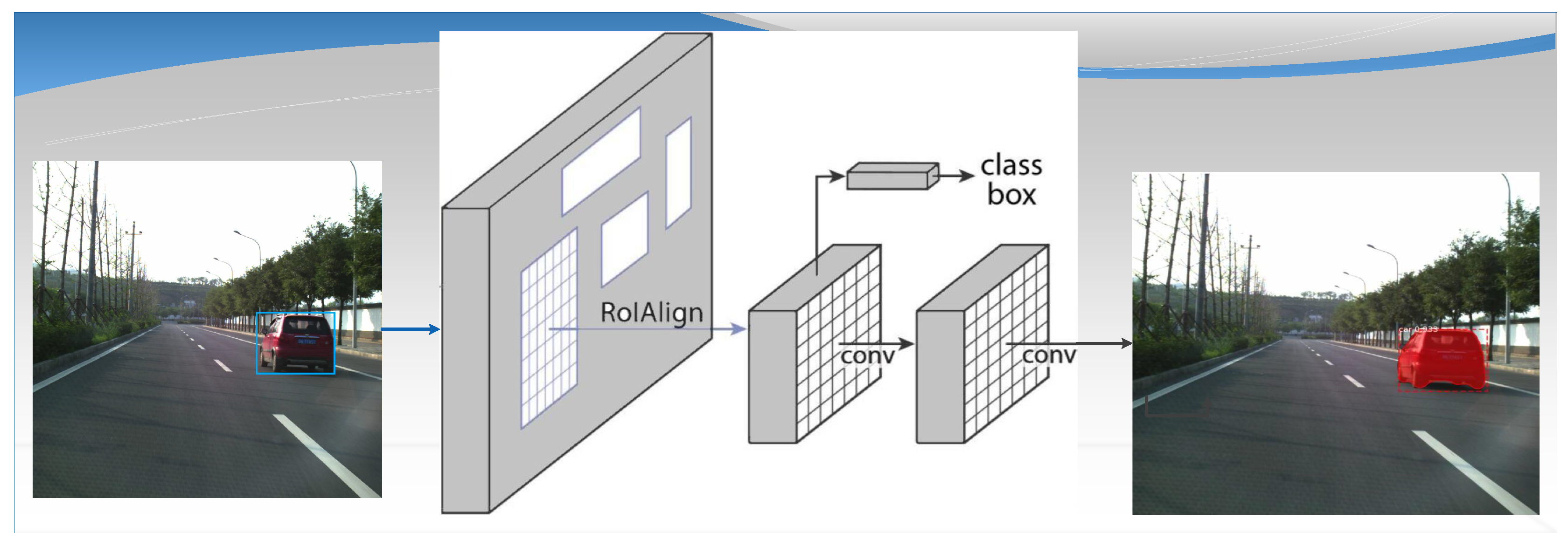
Figure 1. The Mask R-CNN framework for instance segmentation.
Symmetry 11 01081 g001
Figure 2. Algorithm flow.
Symmetry 11 01081 g002
Figure 3. Label category.
Symmetry 11 01081 g003
Figure 4. BDD100K car image.
Symmetry 11 01081 g004
Figure 5. Coordinate transformation process.
Symmetry 11 01081 g005
Figure 6. Small hole imaging model.
Symmetry 11 01081 g006
Figure 7. Monocular vision ranging diagram.
Symmetry 11 01081 g007
Figure 8. Vertical distance.
Symmetry 11 01081 g008
Figure 9. Horizontal distance.
Symmetry 11 01081 g009
Figure 10. Bounding box.
Symmetry 11 01081 g010
Table 1. Test results of BDD100k.
MethodMIoUAverage Running Time
Fast R-CNN78.56%0.74 fps
Faster R-CNN82.06%4.13 fps
Mask R-CNN85.28%4.26 fps
Table 2. Deletion of the time comparison of the RoIAlign layer.
MethodTraining Time/minTest Time/s
Mask R-CNN (RoIAlign)350.3
Mask R-CNN280.2
Table 3. Image location and actual distance from the point to the camera (x-axis).
Serial NumberPixel Coordinates/PixelActual Distance/m
17126.12
256111.01
351613.53
448416.19
544419.85
642623.42
742026.33
839929.37
938232.61
1037335.06
1136248.92
1225051.95
Table 4. Image position and the actual distance from the point to the camera (y-axis).
Serial NumberPixel Coordinates/PixelActual Distance/m
1−205.9−4.04
2292.12.89
3231.12.75
4−246.9−1.96
5145.62.51
6−158.9−1.48
777.62.05
869.62.03
926.11.58
1023.61.57
Table 5. Evaluation criteria for longitudinal curve fitting.
Polynomial OrderSSERMSER-Square
1630.967.947.94
2171.14.360.924
365.862.8690.9707
Table 6. Evaluation criteria for horizontal curve fitting.
Polynomial OrderSSERMSER-Square
21.6827740.4586360.968495
30.2566630.1914840.995195
40.1331770.1489840.997507
Table 7. Evaluation criteria for horizontal curve fitting.
Serial NumberActual x-Axis Distance/mx-Axis Calculation Result/mRelative Error/%Actual y-Axis Distance/my-Axis Calculation Result/mRelative Error/%
1109.25.00.50.5612.0
22018.53.51.51.388.0
33031.24.02.52.269.6
44038.63.53.53.364.0
55047.45.2-0.5-0.4314.0
66065.89.7-1.5-1.416.0
77078.512.4-2.5-2.365.6
88092.315.4-3.5-3.325.1
Table 8. Comparison of the Two Methods.
Actual x-Axis Distance/mFitting Method/mRelative Error/%Geometric Relations Algorithms/mRelative Error/%
109.25.09.010.0
2018.53.522.110.5
3031.24.028.55.0
4038.63.537.85.5
5047.45.253.06.0
6065.89.765.99.8
7078.512.477.610.9
8092.315.489.511.9