On the Structure of Finite Groupoids and Their Representations

Abstract

In this paper, both the structure and the theory of representations of finite groupoids are discussed. A finite connected groupoid turns out to be an extension of the groupoids of pairs of its set of units by its canonical totally disconnected isotropy subgroupoid. An extension of Maschke’s theorem for groups is proved showing that the algebra of a finite groupoid is semisimple and all finite-dimensional linear representations of finite groupoids are completely reducible. The theory of characters for finite-dimensional representations of finite groupoids is developed and it is shown that irreducible representations of the groupoid are in one-to-one correspondence with irreducible representation of its isotropy groups, with an extension of Burnside’s theorem describing the decomposition of the regular representation of a finite groupoid. Some simple examples illustrating these results are exhibited with emphasis on the groupoids interpretation of Schwinger’s description of quantum mechanical systems.

1. Introduction

The theory of groupoids is becoming increasingly widespread not only because of their intrinsic interest, but because of their manifold of applications: consider for instance the references to the significant role played by groupoids in the foundations of physical theories by A. Connes in [1], the recent contributions to the spectral theory of aperiodic systems [2], or the relevant role assigned to them in the mathematical foundations of classical and quantum mechanics in the work by N. Landsman [3]; the combinatorial applications in graph theory [4]; the applications of groupoid theory to geometrical mechanics, control theory (see for instance [5] and references therein) and variational calculus [6]; the recent groupoids based analysis of Schwinger’s algebraic foundation for Quantum Mechanics [7], or the appealing description by A. Weinstein of groupoids as unifying internal and external symmetries [8] extending in a natural way the notion of symmetry groups and groups of transformations with the associated wealth of applications.

In spite of the many treatments of groupoid theory existing in the literature, from the very abstract like the seminal categorical treatment in [9], to the differential geometrical approach in [10], passing through the Harmonic analysis perspective in [11] or the $C^{*}$-algebraic setting [12], we feel that there is a lack of a discussion, as elementary as possible, of the theory and structure of the simplest possible situation, that is, of finite groupoids, that will help researchers in many areas where group theory is useful to effectively use groupoids and their representations.

On the other hand, the theory of linear representations of finite groupoids is interesting enough to deserve a detailed study by itself. We will just mention here that the fundamental representation of the groupoid of pairs of n elements is just the matrix algebra ${\mathbb{C}}^{n\times n}$. Hence, the theory of linear representations of finite groupoids provides a different perspective to the standard algebra of matrices. There is a number of relevant contributions to the theory of linear representations of groupoids describing the notion of measurable and continuous representations (see for instance the aforementioned work by Landsman [3] or [13] and references therein), unitary representations of groupoids and the extension of Mackey’s imprimitivity theorem [14,15,16] or the representation theory of Lie groupoids [17].

In this paper the structure of finite groupoids $\mathbf{G}$ and their linear representations will be discussed by using just elementary methods, most prominently the natural extensions of the theory of characters of finite group representations. The structure of finite groupoids will be explored and it will be proved that finite connected groupoids are extensions (in a sense that will be explained in the main text) of the complete graph groupoid (or the groupoid of pairs) of a finite set by a standard group.

Thus, once the main algebraic properties of finite groupoids are set and the basics of the theory of linear representations are succinctly reviewed, mainly the equivalence of linear representations of groupoids and the theory of R-modules, with R denoting the algebra of the groupoid, the basic theorems of the theory will be stated, and it will be proved that the algebra of a finite groupoid is semisimple, thus establishing the complete reducibility of its representations.

Finally, the properties of the regular representation of a groupoid $\mathbf{G}$ will be discussed, proving that it decomposes as a direct sum of its irreducible representations, each irreducible representation ${\pi }_{\nu }$ arising with multiplicity $p_{\nu }=\left|\mathsf{\Omega }\right|d_{\nu }$, where $\left|\mathsf{\Omega }\right|$ is the cardinal of the space of units $\mathsf{\Omega }$ of the groupoid and $d_{\nu }$ is the dimension of an irreducible representation of the isotropy group $G_x$, $x\in \mathsf{\Omega }$. As in the case of linear representations of groups, characters will be very helpful in proving the main results obtained in this paper and their theory will be described.

A few applications and examples will be discussed. First, and continuing this introduction a brief summary of Schwinger’s approach to the algebra of selective measurements that shows the prominent role played by groupoids in the foundations of quantum mechanics will be provided. Then in Section 5, the situation of the groupoid of a group acting on a given space will be analyzed and a non-trivial groupoid, the groupoid ${\mathfrak{L}}_2$ corresponding to the combinatorial Loyd’s game (see for instance [18]), will be thoroughly discussed.

1.1. Schwinger’s Algebra of Measurements and the Groupoid Picture Of Quantum Mechanics

In his attempts to describe the fundamental structure of quantum mechanical systems, J. Schwinger was searching for a “mathematical language that constituted a symbolic expression of the properties of microscopic measurements” [19].

In Schwinger’s algebraic depiction of a quantum mechanical system, the state of a quantum system is established by performing on it a complete selective measurement (see ([19] Chap. 1)), that is, consider a physical system and denote by $\mathbf{A}$ a family of compatible physical quantities whose outcomes are denoted by $\mathbf{a}$ (that is $\mathbf{a}$ is a real vector whose components are the outcomes of the measurable quantities $A_k$). Then we will call a selective measurement, and we will denote it by $M({\mathbf{a}}^{\prime },\mathbf{a})$, the process that rejects all instances of an ensemble of such physical system whose outcomes are different from $\mathbf{a}$ (when measuring the physical quantity $\mathbf{A}$) and those accepted are changed in such a way that their outcomes of $\mathbf{A}$ become ${\mathbf{a}}^{\prime }$. The symbols $M({\mathbf{a}}^{\prime },\mathbf{a})$ satisfy the following obvious relations:

$$M({\mathbf{a}}^{″},{\mathbf{a}}^{\prime })\circ M({\mathbf{a}}^{\prime },\mathbf{a})=M({\mathbf{a}}^{″},\mathbf{a}),$$

where we consider the natural composition law of selective measurements $M({\mathbf{a}}^{″},{\mathbf{a}}^{\prime })\circ M({\mathbf{a}}^{\prime },\mathbf{a})$ defined as the selective measurement obtained by performing first the selective measurement $M({\mathbf{a}}^{\prime },\mathbf{a})$ and immediately afterwards the selective measurement $M({\mathbf{a}}^{″},{\mathbf{a}}^{\prime })$. Moreover, it is also clear that:

$$M({\mathbf{a}}^{\prime })\circ M({\mathbf{a}}^{\prime },\mathbf{a})=M({\mathbf{a}}^{\prime },\mathbf{a}),M({\mathbf{a}}^{\prime },\mathbf{a})\circ M(\mathbf{a})=M({\mathbf{a}}^{\prime },\mathbf{a}),$$

(1)

where $M(\mathbf{a})$ denotes the selective measurement $M(\mathbf{a},\mathbf{a})$, i.e., the process that accepts the systems whose outcomes are $\mathbf{a}$ leaving them unchanged and rejects all others.

It is clear that performing two selective measurements $M({\mathbf{a}}^{\prime },\mathbf{a})$, and $M({\mathbf{a}}^{‴},{\mathbf{a}}^{″})$ one after the other will produce a selective measurement again only if ${\mathbf{a}}^{″}={\mathbf{a}}^{\prime }$.

Notice that if we have three selective measurements $M(\mathbf{a},{\mathbf{a}}^{\prime })$, $M({\mathbf{a}}^{\prime },{\mathbf{a}}^{″})$ and $M({\mathbf{a}}^{″},{\mathbf{a}}^{‴})$ then, because of the basic definitions, the associativity of the composition law holds:

$$M(\mathbf{a},{\mathbf{a}}^{\prime })\circ (M({\mathbf{a}}^{\prime },{\mathbf{a}}^{″})\circ M({\mathbf{a}}^{″},{\mathbf{a}}^{‴}))=(M(\mathbf{a},{\mathbf{a}}^{\prime })\circ M({\mathbf{a}}^{\prime },{\mathbf{a}}^{″}))\circ M({\mathbf{a}}^{″},{\mathbf{a}}^{‴}).$$

(2)

Finally, it is worth observing that given a measurement symbol $M({\mathbf{a}}^{\prime },\mathbf{a})$ the measurement symbol $M(\mathbf{a},{\mathbf{a}}^{\prime })$ is such that:

$$M({\mathbf{a}}^{\prime },\mathbf{a})\circ M(\mathbf{a},{\mathbf{a}}^{\prime })=M({\mathbf{a}}^{\prime }),M(\mathbf{a},{\mathbf{a}}^{\prime })\circ M({\mathbf{a}}^{\prime },\mathbf{a})=M(\mathbf{a}).$$

(3)

Then we conclude that the composition law of selective measurements determines a groupoid law in the collection ${\mathbf{G}}_{\mathbf{A}}$ of all measurement symbols $M({\mathbf{a}}^{\prime },\mathbf{a})$ associated with the family of compatible observables $\mathbf{A}$, whose objects are the possible outcomes $\mathbf{a}$ of the observables $\mathbf{A}$.

Schwinger’s observation has deep implications. It shows that the algebraic structure of the quantities describing quantum systems is that of the algebra of a groupoid and the groupoid defined by the family of physical transitions between possible outcomes of the system (see [7,20] for a detailed description).

An interesting feature of the groupoids picture of quantum mechanics is that they provide a family of natural representations of Hilbert space associated with the system compared with the standard Dirac’s picture where a Hilbert space is posited. A unitary representation U of the groupoid $\mathbf{G}\rightrightarrows \mathsf{\Omega }$ is a family of Hilbert spaces ${\mathcal{H}}_x$, $x\in \mathsf{\Omega }$ and a family of unitary maps $U(\alpha ):{\mathcal{H}}_x\to {\mathcal{H}}_y$, $\alpha :x\to y\in \mathbf{G}$, such that:

$$U(1_x)=\mathrm{id}{}_{{\mathcal{H}}_x},U(\beta \circ \alpha )=U(\beta )U(\alpha ),(t(\alpha )=s(\beta )),U({\alpha }^{-1})=U{(\alpha )}^{†}.$$

The representation U will be said to be locally finite if the Hilbert spaces ${\mathcal{H}}_x$ are finite dimensional. We will say that the representation U is strongly continuous if the map $\alpha \mapsto U(\alpha )|{\psi }_x\rangle$ is continuous for every $|{\psi }_x\rangle$.

We can form the Hilbert space $\mathcal{H}={⨁}_{x\in \mathsf{\Omega }}{\mathcal{H}}_x$, that will be called the total support space of the representation, and the corresponding associated representation of the $C^{*}$-algebra of the groupoid (We will not worry here with analytical details as we are just going to consider finite groupoids.) $\pi :C^{*}(\mathbf{G})\to \mathcal{B}(\mathcal{H})$, defined as

$$\pi (a)({\oplus }_x|{\psi }_x\rangle )=\sum _{x\in \mathsf{\Omega }}\sum _{\alpha \in \mathbf{G}(x,y)}{a}_{\alpha }U(\alpha )|{\psi }_x\rangle ,$$

$a={\sum }_{\alpha }{a}_{\alpha }\alpha$ is a *-representation. The most conspicuous representation of a groupoid is the fundamental representation ${\pi }_0$ defined by as: ${\pi }_0(\alpha )|x\rangle =|y\rangle$, $\alpha :x\to y$.

1.2. A Simple Example: The Qubit

As an illustrative example, consider what is arguably the simplest non-trivial groupoid structure given by the diagram below, see Figure 1:

This diagram will correspond to a physical system described by a complete family of experimental setups $\mathbf{A}$ producing just two outputs, denoted by + and − in the diagram, and with just one transition $\alpha :+\to -$ among them and its inverse ${\alpha }^{-1}:-\to +$. Notice that the groupoid ${\mathbf{G}}_{\mathbf{A}}$ associated with this diagram has four elements $\{1_{+},1_{-},\alpha ,{\alpha }^{-1}\}$. The groupoid algebra is a complex vector space of dimension 4 generated by $e_1=1_{+}$, $e_2=1_{-}$, $e_3=\alpha$ and $e_4={\alpha }^{-1}$ with structure constants given by the relations:

$$\begin{array}{llll}{e}_1^2=e_1,\hfill & e_2^2=e_2,\hfill & e_1{e}_2=0,\hfill & e_3{e}_4=e_2,\hfill \\ e_4{e}_3=e_1,\hfill & e_3{e}_3=0,\hfill & e_4{e}_4=0,\hfill & e_1{e}_3=0,\hfill \\ e_4{e}_1=0,\hfill & e_1{e}_4=e_4,\hfill & e_3{e}_2=0,\hfill & e_2{e}_3=e_3,\hfill \\ e_2{e}_1=0,\hfill & e_2{e}_4=0,\hfill & e_4{e}_2=e_4,\hfill & e_3{e}_1=e_3.\hfill \end{array}$$

The fundamental representation of the groupoid algebra is supported in the 2-dimensional complex space $\mathcal{H}={\mathbb{C}}^2$ with canonical basis $|+\rangle$, $|-\rangle$. The groupoid elements are represented by operators acting on the canonical basis as:

$$A_{+}|+\rangle =\pi (1_{+})|+\rangle =|+\rangle ,A_{+}|-\rangle =\pi (1_{+})|-\rangle =0,$$

whose associated matrix is:

$$A_{+}=\left[\begin{array}{cc}1& 0\\ 0& 0\end{array}\right].$$

Similarly, we get:

$$A_{-}=\pi (1_{-})=\left[\begin{array}{cc}0& 0\\ 0& 1\end{array}\right],A_{\alpha }=\pi (\alpha )=\left[\begin{array}{cc}0& 0\\ 1& 0\end{array}\right],A_{{\alpha }^{-1}}=\pi ({\alpha }^{-1})=\left[\begin{array}{cc}0& 1\\ 0& 0\end{array}\right],$$

Thus the groupoid algebra can be naturally identified with the algebra of $2\times 2$ complex matrices $M_2(\mathbb{C})$ and the fundamental representation is just provided by the matrix-vector product of matrices and 2-component column vectors of ${\mathbb{C}}^2$.

Observables correspond to elements in the dual space of the algebra of the groupoid that we will identify again with the algebra of $2\times 2$ complex matrices using the standard trace inner product, that is $\langle A,B\rangle =\mathrm{Tr}(A^{†}B)$. Then real observables can be identified with $2\times 2$ Hermitean matrices:

$$A=\left[\begin{array}{cc}{x}_0+x_3& x_1-i{x}_2\\ x_1+i{x}_2& x_0-x_3\end{array}\right]=x_0\mathbf{I}+\mathbf{x}·\sigma =\langle x,\sigma \rangle ,$$

(4)

where ${\sigma }_{\mu }$ denote the standard Pauli $\sigma$-matrices:

$${\sigma }_1=\left[\begin{array}{cc}0& 1\\ 1& 0\end{array}\right],{\sigma }_2=\left[\begin{array}{cc}0& -i\\ i& 0\end{array}\right],{\sigma }_3=\left[\begin{array}{cc}1& 0\\ 0& -1\end{array}\right],$$

together with ${\sigma }_0=\mathbf{I}$, and $\mathbf{x}$ is the vector in ${\mathbb{R}}^3$ with components $(x_1,x_2,x_3)$. Then, the real observable f defined by the Hermitean matrix A above, Equation (4), is given by:

$$f(1_{+})=x_0+x_3,f(1_{-})=x_0-x_3,f(\alpha )=x_1+i{x}_2,f({\alpha }^{-1})=x_1-i{x}_2.$$

Even if we are not going to discuss them in the present paper, we point out that states $\rho$ are defined as normalised positive functionals in $M_2(\mathbb{C})$, and they can be identified with density matrices $\rho ={\rho }^{†}$, $\mathrm{Tr}\rho =1$, $\rho \ge 0$. In this representation, the complete system of observables giving rise to the abstract groupoid described in Figure 1 will be the operator ${\sigma }_3$, that may be identified for instance with the third component $S_z$ of the spin operator $\mathbf{S}$ of an electron. The outcomes of this operator would be its eigenvalues $\pm 1$ (that we have represented by the symbols + and − respectively).

2. Finite Groupoids: A Structure Theorem

2.1. Some Notations and Generalities on Groupoids, Subgroupoids and Connected Groupoids

An abstract groupoid $\mathbf{G}$ is a category whose morphisms are all invertible. A finite groupoid is a groupoid with a finite number of morphisms, hence finite groupoids are concrete groupoids whose morphisms (and hence their objects too) form a finite set. Because the aim of the paper is to discuss the theory of representations of finite groupoids, we assume for the rest of the paper that we will be dealing with finite groupoids even if many of the results presented in what follows can be extended to larger classes of groupoids (like compact ones) as it will be discussed elsewhere. In any case, along the exposition to follow it will be assumed that groupoids are small categories, hence a set theoretical notation for families of morphisms and objects will be used without further mention.

Objects in the groupoid $\mathbf{G}$ will be denoted $x,y$, etc., and its morphisms $\alpha$ by using a convenient diagramatic notation $\alpha :x\to y$, where x is the source of the morphism $\alpha$ and y its target. The family of objects of $\mathbf{G}$ will be denoted by $\mathsf{\Omega }$ and the family of morphisms will be denoted simply by $\mathbf{G}$ again. The source and target maps sending any morphism into its source and target will be denoted by $s:\mathbf{G}\to \mathsf{\Omega }$ and $t:\mathbf{G}\to \mathsf{\Omega }$ respectively. Thus $s(\alpha )=x$, $t(\alpha )=y$ indicates that $\alpha :x\to y$. A groupoid $\mathbf{G}$ over the space of objects $\mathsf{\Omega }$ will be sometimes denoted as $\mathbf{G}\rightrightarrows \mathsf{\Omega }$ to emphasize the source and the target maps $s,t$.

In this paper, the set of morphisms from x to y will be denoted by $\mathbf{G}(y,x)$ (while the standard notation in category theory would be Hom$(x,y)$). Note also the backwards notation for the source and the target of morphisms $\alpha :x\to y$ in the sets $\mathbf{G}(y,x)$. It is clear that $\mathbf{G}(y,x)=s^{-1}(x)\cap t^{-1}(y)$. The number of morphisms of $\mathbf{G}$ will be called the order of $\mathbf{G}$ and denoted by $\left|\mathbf{G}\right|$. Similarly, the number of objects will be denoted by $\left|\mathsf{\Omega }\right|$.

The composition law of the groupoid will be denoted by ∘ and the morphisms $\alpha$ and $\beta$ will be said to be composable if $t(\alpha )=s(\beta )$ in which case the composition will be denoted $\beta \circ \alpha$ (again, notice the backwards convention for the composition), thus $\circ :\mathbf{G}(z,y)\times \mathbf{G}(y,x)\to \mathbf{G}(z,x)$, $\beta \circ \alpha :x\to z$ if $\alpha :x\to y$ and $\beta :y\to z$, thus $\mathbf{G}(z,y)\circ \mathbf{G}(y,x)\subset \mathbf{G}(z,x)$. The set of composable morphisms will be denoted by ${\mathbf{G}}_2$, that is: ${\mathbf{G}}_2=\{(\alpha ,\beta )\in \mathbf{G}\times \mathbf{G}\mid t(\alpha )=s(\beta )\}$.

The composition law ∘ is associative, that is:

$$\gamma \circ (\beta \circ \alpha )=(\gamma \circ \beta )\circ \alpha ,$$

whenever the composition of $\alpha$, $\beta$ and $\gamma$ makes sense.

The unit morphisms of the groupoid will be denoted by $1_x$, $x\in \mathsf{\Omega }$, and they satisfy $1_y\circ \alpha =\alpha$ and $\alpha \circ 1_x=\alpha$ for all $\alpha :x\to y$. The family of units $1_x$ defines a canonical inclusion map $i:\mathsf{\Omega }\to \mathbf{G}$, $i(x)=1_x$, such that $s\circ i=t\circ i={\mathrm{id}}_{\mathsf{\Omega }}$. Any morphism $\alpha :x\to y$ is invertible, its inverse will be denoted by ${\alpha }^{-1}$ and ${\alpha }^{-1}:y\to x$ satisfies ${\alpha }^{-1}\circ \alpha =1_x$ and $\alpha \circ {\alpha }^{-1}=1_y$.

Given an object x of the groupoid $\mathbf{G}$, the family of all morphisms with source and target x, $\alpha :x\to x$, form a group called the isotropy group at x and denoted by $G_x$, that is, $G_x=\mathbf{G}(x,x)$. We will denote by ${\mathbf{G}}_{+}(x)$ the family of all morphisms whose source is x. Similarly ${\mathbf{G}}_{-}(x)$ is the family of all morphisms whose target is x. If ${\mathbf{G}}_{+}(x)$, ${\mathbf{G}}_{-}(y)$ and both sets, then $\mathbf{G}(y,x)={\mathbf{G}}_{+}(x)\cap {\mathbf{G}}_{-}(y)$, and $G_x={\mathbf{G}}_{+}(x)\cap {\mathbf{G}}_{-}(x)$. Notice that if $\mathbf{G}(y,x)$ is non-void, then the isotropy groups $G_y$ and $G_x$ are isomorphic (it suffices to check that if $\alpha :x\to y$, then the map ${\varphi }_{\alpha }:G_x\to G_y$ given by ${\varphi }_{\alpha }({\gamma }_x)=\alpha \circ {\gamma }_x\circ {\alpha }^{-1}$ is a group isomorphism) and $\left|\mathbf{G}(y,x)\right|=|G_x|=|G_y|$.

A subgroupoid $\mathbf{H}$ of the groupoid $\mathbf{G}$ is a groupoid which is a subcategory of $\mathbf{G}$. If $\mathbf{G}$ is a finite groupoid, a subgroupoid $\mathbf{H}$ must be finite too and then, the functor $j:\mathbf{H}\to \mathbf{G}$ that describes $\mathbf{H}$ as a subcategory of $\mathbf{G}$ defines an injective map (denoted with the same symbol) $j:\mathbf{H}\to \mathbf{G}$ that maps morphisms in $\mathbf{H}$ in morphisms in $\mathbf{G}$, ${\alpha }^{\prime }\to \alpha =j({\alpha }^{\prime })$. The functor j defines also an injective map (again denoted with the same symbol) between the objects ${\mathsf{\Omega }}^{\prime }$ of $\mathbf{H}$ and the objects $\mathsf{\Omega }$ of $\mathbf{G}$, that is $j(x^{\prime })=x$. Moreover $j(1_{x^{\prime }})=1_{j(x^{\prime })}=1_x$. The map j satisfies the compatibility condition: $s\circ j=j\circ s^{\prime }$, $t\circ j=j\circ t^{\prime }$, where $s^{\prime }$ and $t^{\prime }$ denote the source and target maps of $\mathbf{H}$ respectively.

Given a subgroupoid $\mathbf{H}$ of $\mathbf{G}\rightrightarrows \mathsf{\Omega }$ with space of objects ${\mathsf{\Omega }}^{\prime }$ smaller than $\mathsf{\Omega }$, we may always consider another subgroupoid $\tilde{\mathbf{H}}$ that extends $\mathbf{H}$ naturally as a subgroupoid of $\mathbf{G}$ whose space of objects is $\mathsf{\Omega }$; $\tilde{\mathbf{H}}$ is defined by simply adding the units $1_x$, $x\in \mathsf{\Omega }\backslash {\mathsf{\Omega }}^{\prime }$ to $\mathbf{H}$. Hence, in what follows a subgroupoid $\mathbf{H}$ of the finite groupoid $\mathbf{G}$ will be assumed to have the same space of objects as $\mathbf{G}$, it will be identified with the subset $j(\mathbf{H})\subset \mathbf{G}$ and its morphisms ${\alpha }^{\prime }$ will be identified with the corresponding morphisms $\alpha =j({\alpha }^{\prime })$ of $\mathbf{G}$.

Given two finite groupoids ${\mathbf{G}}_a$, with object spaces ${\mathsf{\Omega }}_a$, $a=1,2$, we define its coproduct (or direct union) as the groupoid, denoted by ${\mathbf{G}}_1\bigsqcup {\mathbf{G}}_2$, whose morphisms are the disjoint union of the morphisms in ${\mathbf{G}}_1$ and ${\mathbf{G}}_2$ and whose objects are the disjoint union of the objects ${\mathsf{\Omega }}_1$ and ${\mathsf{\Omega }}_2$, the composition law and source and target maps being the obvious ones. It is clear that both ${\mathbf{G}}_1$ and ${\mathbf{G}}_2$ are subgroupoids of ${\mathbf{G}}_1\bigsqcup {\mathbf{G}}_2$ with the obvious inclusion functors $j_a:{\mathbf{G}}_a\to {\mathbf{G}}_1\bigsqcup {\mathbf{G}}_2$, $a=1,2$.

Given an object $x\in \mathsf{\Omega }$, the orbit ${\mathcal{O}}_x$ of the groupoid $\mathbf{G}$ through x is the collection of objects corresponding to the targets of morphisms in ${\mathbf{G}}_{+}(x)$, that is, $y\in {\mathcal{O}}_x$ if there exists $\alpha :x\to y$ or, in other words, ${\mathcal{O}}_x=t({\mathbf{G}}_{+}(x))$. We will say that the groupoid $\mathbf{G}$ is connected (or transitive) if it has just one orbit, in other words, $\mathbf{G}$ is connected if for any $x,y$ objects, there is a morphism $\alpha :x\to y$. Notice that the isotropy groups $G_x$, $G_y$ corresponding to objects $x,y$ in the same orbit are isomorphic (even if not canonically isomorphic).

Let $\mathbf{G}$ be a finite groupoid over the space of objects $\mathsf{\Omega }$. Let us denote by $\mathsf{\Omega }/\mathbf{G}$ the space of orbits ${\mathcal{O}}_x$ of $\mathsf{\Omega }$. The orbits $\mathcal{O}\in \mathsf{\Omega }/\mathbf{G}$ define a partition of $\mathsf{\Omega }$, and we will denote by ${\mathbf{G}}_{\mathcal{O}}$ the restriction of the groupoid $\mathbf{G}$ to the orbit $\mathcal{O}$. The groupoid ${\mathbf{G}}_{\mathcal{O}}$ is a subgroupoid of $\mathbf{G}$ and is a connected groupoid over $\mathcal{O}$. Then the groupoid $\mathbf{G}$ is the direct union of the connected groupoids ${\mathbf{G}}_{\mathcal{O}}$:

$$\mathbf{G}=\underset{\mathcal{O}\in \mathsf{\Omega }/\mathbf{G}}{⨆}{\mathbf{G}}_{\mathcal{O}}.$$

(5)

Thus any groupoid $\mathbf{G}$ is a disjoint union of connected groupoids and its structure will be described by determining the structure of the corresponding connected subgroupoids.

2.2. Quotient Spaces and Normal Subgroupoids

If $\mathbf{H}$ is a subgroupoid of the groupoid $\mathbf{G}$, it determines a canonical equivalence relation on $\mathbf{G}$ as follows: given $\alpha ,{\alpha }^{\prime }$ morphisms in $\mathbf{G}$, $\alpha \sim {\alpha }^{\prime }$ if and only if there exists $\beta ,{\beta }^{\prime }$ morphisms in $\mathbf{H}$ such that ${\alpha }^{\prime }=\beta \circ \alpha \circ {\beta }^{\prime }$. The equivalence classes will be called double groupoid cosets and could be denoted by $\mathbf{H}\alpha \mathbf{H}$. The collection of all double groupoid cosets of $\mathbf{G}$ with respect to $\mathbf{H}$ should be denoted by $\mathbf{H}\backslash \mathbf{G}/\mathbf{H}$ but we will prefer the less cumbersome notation $\mathbf{G}//\mathbf{H}$. If we denote by $\pi$ the canonical projection from $\mathbf{G}$ to the double coset space $\mathbf{G}//\mathbf{H}$, then it is a simple task to realise that $\mathbf{G}//\mathbf{H}$ inherits a groupoid structure from $\mathbf{G}$ such that $\pi$ is a functor if the subgroupoid $\mathbf{H}$ is such that $\alpha \circ \beta \circ {\alpha }^{-1}$ is a morphism in $\mathbf{H}$ for any morphism $\alpha$ in $\mathbf{G}$ such that the previous composition makes sense. Notice that if $\alpha :x\to y$ is such that $\alpha \circ \beta \circ {\alpha }^{-1}$ is well defined, then $\beta$ must be in the isotropy group $G_x$. Hence this leads us to the following definition:

Definition 1.

Let $\mathbf{G}$ be a groupoid, a subgroupoid $\mathbf{H}$ of $\mathbf{G}$ will be called strictly normal if its morphisms are in the isotropy groups $G_x$ of $\mathbf{G}$ and, given $\beta :x\to x$ a morphism in $\mathbf{H}$, then $\alpha \circ \beta \circ {\alpha }^{-1}$ is a morphism in $\mathbf{H}$ for any morphism α in ${\mathbf{G}}_{+}(x)$.

Thus we get the following characterization of quotient groupoids:

Proposition 1.

Let $\mathbf{G}$ be a groupoid and $\mathbf{H}$ a subgroupoid of $\mathbf{G}$. The family of double groupoid cosets $\mathbf{G}//\mathbf{H}$ inherits a groupoid structure such that the natural projection π becomes a functor if the subgroupoid $\mathbf{H}$ is strictly normal.

Proof. 

Notice if $\pi$ is a functor, then $\pi ({\alpha }_1\circ {\alpha }_2)=\pi ({\alpha }_1)\circ \pi ({\alpha }_2)$ for any pair of composable morphisms ${\alpha }_1$ and ${\alpha }_2$ in ${\mathbf{G}}_2$, which determines the composition law in the quotient space $\mathbf{G}//\mathbf{H}$, that is: $(\mathbf{H}{\alpha }_1\mathbf{H})\circ (\mathbf{H}{\alpha }_2\mathbf{H})=\mathbf{H}({\alpha }_1\circ {\alpha }_2)\mathbf{H}$, but then it is clear that such composition law is well-defined if and only if the groupoid is strictly normal because if we select equivalent elements ${\alpha }_a^{\prime }={\beta }_a\circ {\alpha }_a\circ {\beta }_a^{\prime }$, with ${\beta }_a,{\beta }_a^{\prime }$ morphisms in $\mathbf{H}$, $a=1,2$, we will get that:

$$\begin{array}{lll}\hfill {\alpha }_1^{\prime }\circ {\alpha }_2^{\prime }& =& {\beta }_1\circ {\alpha }_1\circ ({\beta }_1^{\prime }\circ {\beta }_2)\circ {\alpha }_2\circ {\beta }_2^{\prime }\hfill \\ & =& {\beta }_1\circ {\alpha }_1\circ {\beta }_3\circ {\alpha }_2\circ {\beta }_2^{\prime }={\beta }_1\circ {\alpha }_1\circ {\alpha }_2\circ ({\alpha }_2^{-1}\circ {\beta }_3\circ {\alpha }_2)\circ {\beta }_2^{\prime },\hfill \end{array}$$

hence, ${\alpha }_1^{\prime }\circ {\alpha }_2^{\prime }\sim {\alpha }_1\circ {\alpha }_2$ iff ${\alpha }_2^{-1}\circ {\beta }_3\circ {\alpha }_2$ is a morphism in $\mathbf{H}$ (notice that ${\beta }_3$ could be any morphism in $\mathbf{H}$). □

Notice that a group G is just a groupoid with a single object e. In such case the unit $1_e$ becomes the neutral element of the group denoted by e again. If G is a group the previously discussed notions of subgroupoids and quotient groupoids become the ordinary ones for groups.

2.3. The Structure of Finite Groupoids

Let us consider a connected groupoid $\mathbf{G}$ over the object space $\mathsf{\Omega }$. The family of isotropy groups $G_x$ of the groupoid $\mathbf{G}$ defines a canonical subgroupoid, denoted in what follows as ${\mathbf{G}}_0$, called the fundamental subgroupoid of $\mathbf{G}$. The groupoid ${\mathbf{G}}_0$ is totally disconnected, that is, its orbits are the objects x themselves. It is clear that the subgroupoid ${\mathbf{G}}_0$ is the direct union of the isotropy groups $G_x$, that is

$${\mathbf{G}}_0=\underset{x\in \mathsf{\Omega }}{⨆}{G}_x.$$

Notice that ${\mathbf{G}}_0$ is a strictly normal subgroupoid of $\mathbf{G}$ and any strictly normal subgroupoid of $\mathbf{G}$ is a subgroupoid of ${\mathbf{G}}_0$. Then the fundamental subgroupoid ${\mathbf{G}}_0$ is the largest strictly normal subgroupoid of $\mathbf{G}$. Hence, as it was discussed in the previous section, because ${\mathbf{G}}_0$ is a strictly normal subgroupoid of $\mathbf{G}$, we can form the corresponding quotient groupoid $\mathbf{G}//{\mathbf{G}}_0$. Then we can prove the following proposition:

Proposition 2.

With the notations above, the groupoid $\mathbf{G}//{\mathbf{G}}_0$ is canonically isomorphic to the groupoid of pairs $\mathsf{\Gamma }(\mathsf{\Omega })$ of the object space Ω.

Proof. 

It is clear that there is a canonical identification between the quotient groupoid $\mathbf{G}//{\mathbf{G}}_0$ and the groupoid of pairs $\mathsf{\Gamma }(\mathsf{\Omega })$ provided by the assignment of the pair $(x,y)$ to the coset ${\mathbf{G}}_0\alpha {\mathbf{G}}_0$ with $\alpha :x\to y$. Then it is easy to check that the previous assignment defines an isomorphism between both groupoids. □

Moreover, if we denote by $ker\pi$ the sugbroupoid of $\mathbf{G}$ defined by those morphisms $\alpha$ such that $\pi (\alpha )$ is a unit element on the quotient groupoid $\mathbf{G}/{\mathbf{G}}_0$, it is clear that $ker\pi ={\mathbf{G}}_0$ and the sequence of functors given by:

$$\mathbf{1}\to {\mathbf{G}}_0\to \mathbf{G}\to \mathsf{\Gamma }(\mathsf{\Omega })\to \mathbf{1},$$

(6)

is exact, that is, $ker\pi =\mathrm{Im}j$ (where $j:{\mathbf{G}}_0\to \mathbf{G}$ is the canonical inclusion and $\mathbf{1}$ just denotes the trivial groupoid over the collection of objects $\mathsf{\Omega }$, i.e., for any object x, it consists of just the unit $1_x$).

Then in analogy with the corresponding terminology for groups, we will say that $\mathbf{G}$ is an extension of $\mathsf{\Gamma }(\mathsf{\Omega })$ by ${\mathbf{G}}_0$.

As an immediate corollary of Proposition 2 we get that if $\mathbf{G}$ is a finite groupoid, then because of (5):

$$\left|\mathbf{G}\right|=\sum _{\mathcal{O}\in \mathsf{\Omega }/\mathbf{G}}|G_x{\left|\right|\mathcal{O}|}^2.$$

(7)

where the sum is taken over the space of orbits $\mathsf{\Omega }/\mathbf{G}$ of the groupoid $\mathbf{G}$ with $G_x$ the isotropy group of any object x in $\mathcal{O}$ and $\left|\mathcal{O}\right|$ denotes the cardinal of the orbit $\mathcal{O}$.

Notice that the structure theorem above becomes void for groups as the fundamental subgroupoid of a group G is the group G itself and the corresponding quotient space consists of a single element.

3. Representations of Finite Groupoids and Associative Algebras

3.1. Linear Representations of Groupoids

We will denote by $\mathbf{Vect}$ the category of linear spaces whose objects are complex linear spaces V and whose morphisms are linear maps $L:V\to W$. The subcategory of finite-dimensional linear spaces will be denoted as $\mathbf{FinVect}$.

Definition 2.

A linear representation of a groupoid $\mathbf{G}\rightrightarrows \mathsf{\Omega }$ is a functor R from the category $\mathbf{G}$ to the category $\mathbf{Vect}$ of linear spaces. A finite-dimensional representation of a groupoid $\mathbf{G}\rightrightarrows \mathsf{\Omega }$ is a functor R from the category $\mathbf{G}$ to the category $\mathbf{FinVect}$ of finite dimensional linear spaces. A linear representation will be denoted as $R:\mathbf{G}\to \mathbf{Vect}$.

More specifically, if R is a finite-dimensional representation of the groupoid $\mathbf{G}$, the functor R assigns a finite dimensional linear space $V_x:=R(x)$ to any object $x\in \mathsf{\Omega }$ and a linear map $R(\alpha ):V_x\to V_y$, to any morphism $\alpha :x\to y$ in the groupoid, in such a way that $R(\beta \circ \alpha )=R(\beta )R(\alpha )$ for every composable pair $\alpha$, $\beta$ and $R(1_x)={\mathrm{id}}_{V_x}$ is the identity map on each linear space $V_x$.

Because of the decomposition (5), we can restrict ourselves to consider connected groupoids. Notice that if the groupoid is connected then all spaces $V_x=R(x)$ corresponding to the linear representation R are isomorphic, hence the linear spaces defined by any representation of a finite groupoid are isomorphic on each orbit of the groupoid and they possess the same dimension n if the representation is finite dimensional. We will call this number the dimension of the representation R of the finite connected groupoid. Notice that the dimension could vary from connected component to connected component.

Given a representation R of a finite groupoid $\mathbf{G}$, we will call the linear space $V={⨁}_{x\in \mathsf{\Omega }}{V}_x$ the total space of the representation. Notice that if $\mathbf{G}$ is connected and R is finite dimensional, $dimV=\left|\mathsf{\Omega }\right|n$, with n the dimension of the representation.

In particular, if the groupoid $\mathbf{G}$ is a group, i.e., it possesses just one object (that may be identified with the neutral element of the group), a linear representation R of the groupoid becomes a standard linear representation of the group, that is $R(g):V\to V$, V is a linear space (the one associated with the neutral element), $R(g)$ is a linear map such that $R(g^{-1})=R{(g)}^{-1}$ for any element g in the group, and $R(g{g}^{\prime })=R(g)R(g^{\prime })$ for any $g,g^{\prime }$ elements in the group $\mathbf{G}$.

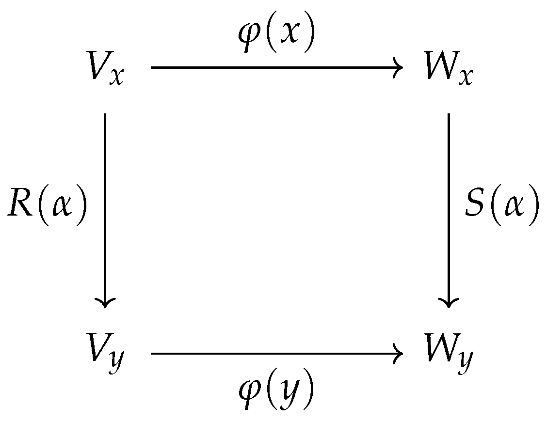
There is a ‘natural’ notion of equivalence between linear representations of a groupoid and it is given by the notion of natural transformations among functors. More specifically, a natural transformation $\phi :R\Rightarrow S$ between the functors R and S defining two linear representations of $\mathbf{G}$, assigns to any object x of the groupoid $\mathbf{G}$ a linear map $\phi (x):R(x)=V_x\to S(x)=W_x$ such that the diagram below (Figure 2) is commutative, that is, $S(\alpha )\circ \phi (x)=\phi (y)\circ R(\alpha )$ for any $\alpha :x\to y$.

If we are given two natural transformations $\phi :R\Rightarrow S$ and $\psi :S\Rightarrow T$ the composition of them, $\psi \circ \phi :R\Rightarrow T$, is defined in the obvious way: $(\psi \circ \phi )(x)=\psi (x)\circ \phi (x)$ for all objects x.

The natural transformation $\phi :R\Rightarrow S$ is said to be invertible if there exists another natural transformation ${\phi }^{-1}:S\Rightarrow R$, such that ${\phi }^{-1}\circ \phi ={\mathbf{1}}_R$, with ${\mathbf{1}}_R$ the trivial natural transformation ${\mathbf{1}}_R:R\to R$ given by ${\mathbf{1}}_R(x)={\mathrm{id}}_{R(x)}$. Then we can state the notion of equivalence of two linear representations R and S as follows:

Definition 3.

Given two linear representations $R,S:\mathbf{G}\to \mathbf{Vect}$ we will say that R and S are equivalent if there exists an invertible natural transformation $\phi :R\Rightarrow S$ between the functors R and S.

Again, the restriction of the notion of equivalence of linear representations to the class of groups provides the standard notion of equivalence of linear representations of groups.

The family of linear representations of groupoids is a category itself whose objects are the representations R and its morphisms are natural transformations $\phi :R\Rightarrow S$. We may consider the category $\mathbf{Rep}(\mathbf{G})$ whose objects are equivalence classes of representations and the corresponding induced natural transformations as morphisms. This category is the structure we would like to study for a given groupoid $\mathbf{G}$ as it provides all possible linear ‘snapshots’ of the given abstract groupoid. We will find out that, similar to the theory of linear representations of finite groups, this category can be described completely and it is constructed from a finite number of ‘elementary’ blocks, the irreducible representations of the groupoid.

A subrepresentation $R^{\prime }$ of a linear representation R of the groupoid $\mathbf{G}$ is a functor $R^{\prime }:\mathbf{G}\to \mathbf{Vect}$ such that for each object x, $V_x^{\prime }=R^{\prime }(x)\subset R(x)=V_x$, and the restriction of the linear map $R(\alpha )$ to the subspace $V_x^{\prime }$ coincides with $R^{\prime }(\alpha )$, in such case we will write $R^{\prime }\subset R$. Notice that if $R^{\prime }\subset R$ is a subrepresentation of R, then the subspaces $V_x^{\prime }=R^{\prime }(x)\subset V_x=R(x)$ are invariant under $\mathbf{G}$ in the sense that $R(\alpha )v_x\in V_y^{\prime }$ for any vector $v_x\in V_x^{\prime }$ and $\alpha :x\to y$. Notice that if $R^{\prime }\subset R$ is a subrepresentation of R, then we may define a representation of $\mathbf{G}$ on the quotient spaces $V_x/V_x^{\prime }$, by means of $T(\alpha )(v_x+V_x^{\prime })=R(\alpha )(v_x)+V_x^{\prime }$, $v_x\in V_x$. We will call this representation the quotient representation of R by $R^{\prime }$ and we denote it by $R/R^{\prime }$.

Any representation R has two trivial subrepresentations: R itself and the zero representation, that is, the functor $\mathbf{0}$ that assigns the zero vector space to any object. Any subrepresentation of a linear representation R of the groupoid $\mathbf{G}$ different from the two trivial subrepresentations R and $\mathbf{0}$ will be called a proper subrepresentation. We will be interested in representations that do not possess proper subrepresentations.

Definition 4.

A representation R of a groupoid $\mathbf{G}$ will be said to be irreducible if it has no proper subrepresentations.

Notice that any irreducible representation of a finite groupoid is finite-dimensional. In fact, if $R:\mathbf{G}\to \mathbf{Vect}$ is irreducible, we can choose a non-zero vector $v_x$ in each space $V_x$ for each $x\in \mathsf{\Omega }$ and define the space $\mathrm{span}\{R(\alpha )v_x\mid \alpha \in {\mathbf{G}}_{-}(x)\}$ which clearly constitutes a finite-dimensional subrepresentation of R. Moreover, a simple induction argument shows that any finite-dimensional representation contains an irreducible representation.

Given two linear representations R, S of the groupoid $\mathbf{G}$, we may define its direct sum $R\oplus S$ and tensor product $R\otimes S$ in a similar way as in the case of groups. These operations induce natural operations on the category $\mathbf{Rep}(\mathbf{G})$. We will not use this structure in what follows as we are not intending to address the extension of the Tannaka-Krein duality (see for instance [21] and references therein) to the category of groupoids, a problem that will be dealt with elsewhere.

More specifically, we define the direct sum $R\oplus S$ of two representations R, S as the linear representation of the groupoid $\mathbf{G}$ determined by the functor that assigns the linear space $R(x)\oplus S(x)=V_x\oplus W_x$ ($R(x)=V_x$ and $S(x)=W_x$) to any object x, and a linear map $R(\alpha )\oplus S(\alpha ):V_x\oplus W_x\to V_y\oplus W_y$ to any $\alpha :x\to y$. Similarly, we define $R\otimes S$ as the linear representation of the groupoid $\mathbf{G}$ determined by the functor that assigns the linear space $R(x)\otimes S(x)=V_x\otimes W_x$ to any object x and the linear map $R(\alpha )\otimes S(\alpha ):V_x\otimes W_x\to V_y\otimes W_y$, to any $\alpha :x\to y$.

Definition 5.

A linear representation R of the groupoid $\mathbf{G}$ will be said to be decomposable if given a subrepresentation $R^{\prime }$ of R there exists another subrepresentation $R^{″}$ of R such that $R=R^{\prime }\oplus R^{″}$. We will say that the representation R is indecomposable if it is not decomposable.

Notice that any irreducible representation is indecomposable, however, the converse is not necessarily true.

Definition 6.

A linear representation $R:\mathbf{G}\to \mathbf{Vect}$ of a groupoid $\mathbf{G}$ will be said to be completely reducible if it is equivalent to a direct sum of irreducible representations. In particular, a finite dimensional linear representation $R:\mathbf{G}\to \mathbf{FinVect}$ will be completely reducible if it is equivalent to a finite direct sum $R_1\oplus \cdots \oplus R_r$ of irreducible representations of $\mathbf{G}$.

The following theorem shows that any finite-dimensional representation is completely reducible.

Theorem 1.

Any finite-dimensional linear representation R of a finite groupoid $\mathbf{G}$ is completely reducible and is equivalent to the direct sum of irreducible representations whose factors and multiplicities are uniquely determined. Moreover, any indecomposable finite-dimensional linear representation of a finite groupoid is irreducible.

Hence, if $\mathbf{G}$ is a finite groupoid, as a consequence of the previous theorem we can concentrate on the study of its finite-dimensional linear representations and its decomposition in irreducible ones.

The theorem is a consequence of the following Lemmas, the groupoid analogue of the Jordan-Hölder theorem in the case of groups, whose proofs follows a similar pattern (see for instance [22,23]), the theorem proving that the algebra of a finite groupoid is semisimple, Theorem 3, and the characterization of semisimplicity, Theorem 2 below.

Given a linear representation $R:\mathbf{G}\to \mathbf{Vect}$, a finite filtration of R is a sequence of subrepresentations $R_k$, $k=0,1,\dots ,n$, such that $\mathbf{0}=R_0\subset R_1\subset R_2\subset \cdots \subset R_{n-1}\subset R_n=R$.

Lemma 1.

Any finite dimensional representation R of a finite groupoid $\mathbf{G}$ admits a finite filtration $\mathbf{0}=R_0\subset R_1\subset \cdots \subset R_n=R$ such that the successive quotients $R_i/R_{i-1}$ are irreducible.

Proof. 

We will assume that the groupoid is connected and the proof is by induction in n, the dimension of the representation. The statement is obviously true for $n=1$.

Let R be a finite dimensional representation. If R is not irreducible, let $R^{\prime }\subset R$ be an irreducible subrepresentation. Then consider the representation $R/R^{\prime }$ and apply the induction hypothesis. □

Proposition 3.

Let R be a finite-dimensional representation of the finite groupoid $\mathbf{G}$. Let $\mathbf{0}=R_0\subset R_1\subset R_2\subset \cdots \subset R_{n-1}\subset R_n=R$ and $\mathbf{0}=R_0^{\prime }\subset R_1^{\prime }\subset R_2^{\prime }\subset \cdots \subset R_{m-1}^{\prime }\subset R_m^{\prime }=R$ be filtrations of R such that the representations $R_i/R_{i-1}$ and $R_k^{\prime }/R_{k-1}^{\prime }$ are irreducible for all i and k (in particular $R_1$ and $R_1^{\prime }$ are irreducible). Then $n=m$ and there exists a permutation σ such that $R_{\sigma (i)}$ is equivalent to $R_i^{\prime }$.

Proof. 

Again, assuming that $\mathbf{G}$ is connected, the proof is by induction on the dimension of the representation n. The case $n=1$ is trivial.

Suppose that $n>1$ and $R_1$ is not equivalent to $R_1^{\prime }$ (if $R_1$ and $R_1^{\prime }$ were equivalent, we apply the induction hypothesis). In such case the intersection of the subspaces corresponding to $R_1$ and $R_1^{\prime }$ is zero, that is $R_1(x)\cap R_1^{\prime }(x)=\mathbf{0}$ (if not, the intersection will define a proper subrepresentation of both $R_1$ and $R_1^{\prime }$ in contradiction with the assumption that they are irreducible). Then we can consider the subrepresentation $R_1\oplus R_1^{\prime }\subset R$ and the quotient $R/(R_1\oplus R_1^{\prime })$. Consider a filtration $\mathbf{0}=T_0\subset T_1\subset \cdots \subset T_p=R/(R_1\oplus R_1^{\prime })$ such that the quotients $S_i=T_i/T_{i-1}$ are irreducible (that exists because of Lemma 1). Then $R/R_1$ has a filtration with successive quotients $R_1^{\prime },T_1,\dots ,T_p$ and another with successive quotients $R_2/R_1,\dots ,R_n/R_{n-1}$ and $R/R_1^{\prime }$ has two filtrations with successive quotients $R_1,T_1,\dots ,T_p$ and $R_2^{\prime }/R_1^{\prime },\dots ,R_m^{\prime }/R_{m-1}^{\prime }$. Then by the induction hypothesis, the collection of irreducible representations on both filtrations coincide. □

3.2. The Groupoid Algebra and Linear Representations of Groupoids

Given a finite groupoid $\mathbf{G}$, we will denote by $\mathbb{C}\left[\mathbf{G}\right]$ the finite dimensional *-algebra generated by the elements $\alpha$ in the groupoid and relations provided by the groupoid composition law, that is, elements $\mathit{a}$ of the algebra $\mathbb{C}\left[\mathbf{G}\right]$ are formal linear combinations of elements in $\mathbf{G}$ with complex coefficients: $\mathit{a}={\sum }_{\alpha \in \mathbf{G}}{a}_{\alpha }\alpha$, $a_{\alpha }\in \mathbb{C}$. The composition law is given by:

$$\mathit{a}·\mathit{b}=\sum _{(\alpha ,\beta )\in {\mathbf{G}}_2}{a}_{\alpha }{b}_{\beta }\alpha \circ \beta ,$$

(8)

with $\mathit{a}={\sum }_{\alpha }{a}_{\alpha }\alpha$, $\mathit{b}={\sum }_{\beta }{b}_{\beta }\beta$ (notice that the composition of morphisms on the r.h.s. of Equation (8) is only among composable pairs $\alpha$, $\beta$).

The algebra $\mathbb{C}\left[\mathbf{G}\right]$ is a unital associative algebra. The unit element is given by $\mathbf{1}={\sum }_{x\in \mathsf{\Omega }}{1}_x$. There is, in addition, a natural antilinear involution map * defined as:

$$\mathit{a}=\sum _{\alpha }{a}_{\alpha }\alpha \mapsto {\mathit{a}}^{*}=\sum _{\alpha }{\overline{a}}_{\alpha }{\alpha }^{-1}.$$

The unital associative algebra $\mathbb{C}\left[\mathbf{G}\right]$ equipped with the involution * becomes a *-algebra. Even more, there is a canonical norm $\left|\right|·\left|\right|$ in $\mathbb{C}\left[\mathbf{G}\right]$ that makes it into a $C^{*}$-algebra (even if we will not use this structure in the current work).

The natural correspondence between linear representations of the groupoid $\mathbf{G}$ and $\mathbb{C}\left[\mathbf{G}\right]$-modules allows us to use the structure of the algebra $\mathbb{C}\left[\mathbf{G}\right]$ to study the linear representations of $\mathbf{G}$. More specifically, given a linear representation R of the finite groupoid $\mathbf{G}$, there is a $\mathbb{C}\left[\mathbf{G}\right]$-module V associated with it. The linear space V is the total space of the representation R given by $V={⨁}_{x\in \mathsf{\Omega }}{V}_x$ and the action of the algebra $\mathbb{C}\left[\mathbf{G}\right]$ on V is given by:

$$\mathit{a}·v=\underset{x\in \mathsf{\Omega }}{⨁}\left(\sum _{\alpha \in G_{+}(x)}{a}_{\alpha }R(\alpha )v_x\right),$$

where $v={⨁}_x{v}_x$ and $\mathit{a}={\sum }_{\alpha }{a}_{\alpha }\alpha$, in particular $\alpha ·v_x=R(\alpha )(v_x)$.

Conversely, if V is a finite-dimensional $\mathbb{C}\left[\mathbf{G}\right]$-module, consider any element $\mathit{a}\in \mathbb{C}\left[\mathbf{G}\right]$ as a linear map on V. The units $1_x$ of the groupoid $\mathbf{G}$ define a family of projectors $P_x$ on V, $P_x(v)=1_x·v$. Notice that $P_x^2=P_x$ and $P_x{P}_y=\delta (x,y)P_x$. If we denote by $V_x$ the range of the projector $P_x$, then $V={⨁}_{x\in \mathsf{\Omega }}{V}_x$ and the family of maps $R(\alpha ):V_x\to V_y$, $\alpha :x\to y$, defined as $R(\alpha )v_x=\alpha ·v_x$, $v_x\in V_x$ defines a linear representation of the groupoid $\mathbf{G}$.

Hence, any linear representation $R:\mathbf{G}\to \mathbf{FinVect}$ defines a $\mathbb{C}\left[\mathbf{G}\right]$-module V and a linear map $R:\mathbb{C}\left[\mathbf{G}\right]\to \mathrm{End}(V)$, $R(\mathit{a})v=\mathit{a}·v$. In what follows we will use these notions interchangeably.

The previous identification of linear representations of the groupoid $\mathbf{G}$ and $\mathbb{C}\left[\mathbf{G}\right]$-modules extends to the rest of the definitions, in particular we recall that a linear representation R is irreducible iff the corresponding $\mathbb{C}\left[\mathbf{G}\right]$-module V is simple (i.e., it has no proper submodules).

3.3. The Fundamental Representation of a Finite Groupoid

In this section we will discuss the fundamental representation of a finite groupoid leaving to Section 4.3 the discussion on its left and right regular representations.

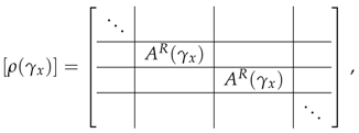
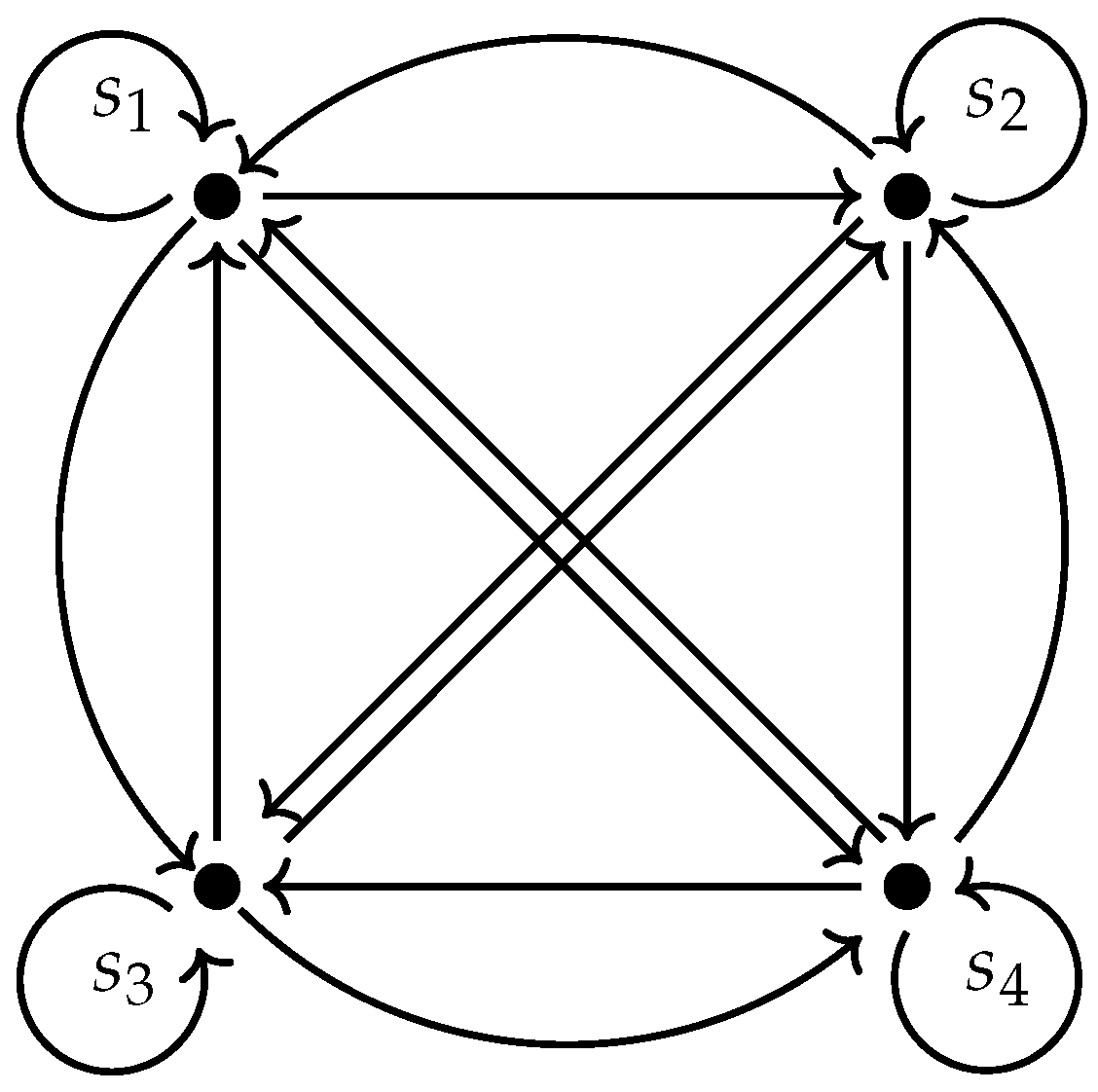
The fundamental representation ${\pi }_0:\mathbb{C}\left[\mathbf{G}\right]\to \mathrm{End}({\mathcal{H}}_{\mathsf{\Omega }})$ of the finite groupoid $\mathbf{G}\rightrightarrows \mathsf{\Omega }$, is supported on the linear space ${\mathcal{H}}_{\mathsf{\Omega }}$ freely generated by the elements of $\mathsf{\Omega }$, that is, vectors in ${\mathcal{H}}_{\mathsf{\Omega }}$ are formal linear combinations $\psi ={\sum }_{x\in \mathsf{\Omega }}{\psi }_{x}x$, ${\psi }_x\in \mathbb{C}$.

The linear space ${\mathcal{H}}_{\mathsf{\Omega }}$ has dimension $\left|\mathsf{\Omega }\right|$ and carries a canonical basis $\{x\}$ given by the elements x of $\mathsf{\Omega }$ themselves. The existence of the canonical basis $\{x\}$ allows us to introduce a natural inner product $\langle ·,·\rangle$ such that the vectors x form an orthonormal basis, that is $\langle x,y\rangle =\delta (x,y)$.

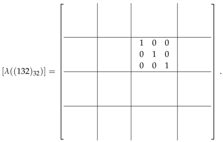
The representation ${\pi }_0$ is defined as follows: let $\alpha :x\to y$ a groupoid morphism, then define the linear map

$${\pi }_0(\alpha )\left(\sum _{z\in \mathsf{\Omega }}{\psi }_{z}z\right)=\sum _{z\in \mathsf{\Omega }}{\psi }_z\delta (x,z)y,$$

i.e., the linear map ${\pi }_0(\alpha )$ transforms the element x of the canonical basis to y and all others to zero.

It is simple to check that the fundamental representation ${\pi }_0$ is unitary, that is for any unitary element $\mathit{a}$ in $\mathbb{C}\left[\mathbf{G}\right]$ (${\mathit{a}}^{*}·\mathit{a}=\mathit{a}·{\mathit{a}}^{*}=\mathbf{1}$), ${\pi }_0(\mathit{a})$ is a unitary operator: ${\pi }_0{(\mathit{a})}^{-1}={\pi }_0{(\mathit{a})}^{†}$, where ${(·)}^{†}$ denotes the Hermitean conjugate (or adjoint) with respect to the inner product $\langle ·,·\rangle$. The previous assertion follows easily from the fact that ${\pi }_0({\mathit{a}}^{*})={\pi }_0{(\mathit{a})}^{†}$.

Proposition 4.

Let $\mathbf{G}$ be a finite connected groupoid, then the fundamental representation ${\pi }_0$ is irreducible.

Proof. 

Suppose that $V\subset {\mathcal{H}}_{\mathsf{\Omega }}$ is a $\mathbb{C}\left[\mathbf{G}\right]$-submodule, then $V_x=P_x(V)$, with $P_x={\pi }_0(1_x)$ the corresponding projector on ${\mathcal{H}}_{\mathsf{\Omega }}$, defines a subrepresentation of ${\pi }_0$. However, either $V_x$ is the zero space or $\mathbb{C}x$ (because $P_x({\mathcal{H}}_{\mathsf{\Omega }})=\mathbb{C}x$). If $V_x\ne \{\mathbf{0}\}$, then given $y\in \mathsf{\Omega }$, $V_y\ne \{\mathbf{0}\}$ because there is $\alpha :x\to y$, and $y=\alpha ·x={\pi }_0(\alpha )(x)\in V_y$. Then ${\oplus }_{x\in \mathsf{\Omega }}{V}_x=V={\mathcal{H}}_{\mathsf{\Omega }}$. □

3.4. Semisimplicity

The main theorem concluding the discussion in this section is that the algebra of a finite groupoid is semisimple. Given an algebra A, its Jacobson radical $\mathrm{Rad}(A)$ is the largest nilpotent two-sided ideal of A. Then, let us recall that a semisimple associative algebra is an algebra such that its Jacobson radical is zero. The following theorem summarizes a number of properties of finite-dimensional algebras equivalent to semisimplicity (see for instance ([23] Ch. 3)).

Theorem 2.

For a finite dimensional algebra A, they are equivalent:

i. 

A is semisimple.

ii. 

Any finite dimensional representation of A is completely reducible.

iii. 

Any A-submodule U of an A-module V has supplementary factor, that is, there is an A-submodule W such that $V=U\oplus W$.

Then we may prove the main theorem in this section:

Theorem 3.

The groupoid algebra $\mathbb{C}\left[\mathbf{G}\right]$ of a finite groupoid $\mathbf{G}$ is semisimple.

Proof. 

Let V be a $\mathbb{C}\left[\mathbf{G}\right]$-module and U a $\mathbb{C}\left[\mathbf{G}\right]$-submodule. Let $U^{\prime }$ be a supplementary subspace to U, that is, $V=U\oplus U^{\prime }$. Let $P_U:V\to U$ be the projector onto U parallel to $U^{\prime }$, that is $P_U^2=P_U$, $P_U{\mid }_U={\mathrm{id}}_U$, $ker{P}_U=U^{\prime }$. Define:

$$P(v)=\frac{1}{\left|\mathbf{G}\right|}\sum _{\alpha \in \mathbf{G}}{\alpha }^{-1}·(P_U(\alpha ·v)),$$

or, more compactly,

$$P=\frac{1}{\left|\mathbf{G}\right|}\sum _{\alpha \in \mathbf{G}}{\alpha }^{-1}{P}_U\alpha .$$

Clearly P is a projector $P^2=P$, $P{\mid }_U={\mathrm{id}}_U$.

Consider now the subspace $W=kerP$ which is a supplementary subspace to U: $V=U\oplus W$.

Then we notice that W is a $\mathbb{C}\left[\mathbf{G}\right]$-submodule. For any $v\in W=kerP$:

$$\begin{array}{lll}\hfill P(\beta ·v)& =& \frac{1}{\left|\mathbf{G}\right|}\sum _{\alpha \in \mathbf{G}}{\alpha }^{-1}·P_U(\alpha ·\beta ·v)=\frac{1}{\left|\mathbf{G}\right|}\sum _{\alpha \in \mathbf{G}}{\alpha }^{-1}·P_U((\alpha ·\beta )v)\hfill \\ & =& \frac{1}{\left|\mathbf{G}\right|}\sum _{{\alpha }^{\prime }\in \mathbf{G}}\beta ·{\alpha }^{\prime -1}·P_U({\alpha }^{\prime }·v)=\beta ·\left(\frac{1}{\left|\mathbf{G}\right|}\sum _{{\alpha }^{\prime }\in \mathbf{G}}{\alpha }^{\prime -1}·P_U({\alpha }^{\prime }·v)\right)\hfill \\ & =& \beta ·(Pv)=0.\hfill \end{array}$$

Then, because of the characterization of semisimple algebras provided by Theorem 2, the algebra $\mathbb{C}\left[\mathbf{G}\right]$ of the groupoid $\mathbf{G}$ is semisimple. □

As an immediate consequence of Theorem 3, we obtain the extension of Wedderburn’s theorem for groupoids:

Corollary 1.

Let $\mathbf{G}$ be a finite groupoid. Then:

$$\mathbb{C}\left[\mathbf{G}\right]\cong M_{n_1}(\mathbb{C})\cdots \oplus M_{n_r}(\mathbb{C}),$$

and $\left|\mathbf{G}\right|={\sum }_k{n}_k^2$.

If the groupoid $\mathbf{G}$ is a finite group, the previous corollary and theorems reproduce Maschke’s theorem, a central result in the theory of linear representations of groups. Actually, in that vein, we may refine the last corollary by stating that the factors appearing in the decomposition of the groupoid algebra are in one-to-one correspondence with the irreducible representations of the groupoid and they provide the canonical decomposition of its regular representation. These aspects will be the subject of the following section.

4. The Structure of the Regular Representation of a Groupoid

In this section the simple factors in the decomposition of the algebra of the finite groupoid $\mathbf{G}$ will be identified explicitly inside the regular representation of the algebra. It will be shown that there is a one-to-one correspondence between irreducible representations of the groupoid ${\pi }_{\nu }$ and the irreducible representations ${\mu }_{\nu }$ of the isotropy groups, and that the regular representation of a finite groupoid contains each irreducible representation ${\pi }_{\nu }$ with multiplicity its dimension, $d_{\nu }\left|\mathsf{\Omega }\right|$, with $d_{\nu }$ the dimension of an irreducible representation ${\mu }_{\nu }$ of the isotropy group $G_x$. In order to develop these ideas and to prove the announced results, we will succinctly review the theory of characters of representations of finite dimensional algebras adapted to the situation at hand.

4.1. Characters

An important tool in the description of representations of finite dimensional algebras is provided by their characters. The character $\chi$ of a finite-dimensional representation $R:\mathbb{C}\left[\mathbf{G}\right]\to \mathrm{End}(V)$ will be defined in the standard way, that is

$${\chi }_R(\mathit{a})=\mathrm{Tr}(R(\mathit{a})),$$

for any $\mathit{a}\in \mathbb{C}\left[\mathbf{G}\right]$. Characters are central functions on the groupoid algebra, that is:

$${\chi }_R(\mathit{a}·\mathit{b})={\chi }_R(\mathit{b}·\mathit{a}),$$

for all $\mathit{a}$, $\mathit{b}$ in $\mathbb{C}\left[\mathbf{G}\right]$. Notice that if $\mathit{u}$ is a unitary element in the groupoid algebra, then $\chi ({\mathit{u}}^{-1})=\chi ({\mathit{u}}^{*})=\overline{\chi (\mathit{u})}$.

Denoting by $\mathbb{C}{\left[\mathbf{G}\right]}^{\prime }$ the derived algebra of the groupoid algebra (or the linear span of commutators $[\mathit{a},\mathit{b}]=\mathit{a}·\mathit{b}-\mathit{b}·\mathit{a}$, for all $\mathit{a},\mathit{b}\in \mathbb{C}\left[\mathbf{G}\right]$), it is clear that a character $\chi$ induces a map (denoted with the same symbol by a small abuse of notation) $\chi :\mathbb{C}\left[\mathbf{G}\right]/\mathbb{C}{\left[\mathbf{G}\right]}^{\prime }\to \mathbb{C}$.

Then, it is not hard to prove that characters of different irreducible finite dimensional representations of $\mathbb{C}\left[\mathbf{G}\right]$ are linearly independent and that these characters form a linear basis of the dual space of $\mathbb{C}\left[\mathbf{G}\right]/\mathbb{C}{\left[\mathbf{G}\right]}^{\prime }$. Actually, the last statement is true for any finite dimensional semisimple algebra, and because Theorem 3 this is actually the situation for $\mathbb{C}\left[\mathbf{G}\right]$.

In the particular instance of the algebra of the groupoid $\mathbf{G}$, we may consider the characters as functions defined in the groupoid itself, that is:

$${\chi }_R:\mathbf{G}\to \mathbb{C},{\chi }_R(\alpha )=\mathrm{Tr}(R(\alpha )).$$

In what follows we will use characters in this sense.

Notice that if ${\chi }_R$ and ${\chi }_S$ denote the characters of the representations R and S respectively, then ${\chi }_{R\oplus S}={\chi }_R+{\chi }_S$. Moreover, ${\chi }_{R\otimes S}={\chi }_R·{\chi }_S$ and ${\chi }_{R^{*}}={\overline{\chi }}_R$. The last identity requires some comments. Given the representation $R:\mathbb{C}\left[\mathbf{G}\right]\to \mathrm{End}(V)$ we denote by $R^{*}$ the representation $R^{*}:\mathbb{C}\left[\mathbf{G}\right]\to \mathrm{End}(V^{*})$ given by $R^{*}(\mathit{a})(v^{*})=R{({\mathit{a}}^{*})}^{*}(v^{*})$, $v^{*}\in V^{*}$, where $\langle R{({\mathit{a}}^{*})}^{*}(v^{*}),v\rangle =\langle v^{*},R({\mathit{a}}^{*})(v)\rangle$, for any $v\in V$ and $\langle ·,·\rangle$ denotes the natural pairing between $V^{*}$ and V.

4.2. Orthogonality of Characters

The previous observations were valid for characters of representations of arbitrary finite-dimensional semisimple algebras, however, in the particular instance of the algebra of a finite groupoid we can be more specific. Actually, we have that if R is a representation of the groupoid algebra $\mathbb{C}\left[\mathbf{G}\right]$ on the linear space V, i.e., V is an $\mathbb{C}\left[\mathbf{G}\right]$-module, then the character ${\chi }_R$ of the representation R is given by:

$${\chi }_R(\mathit{a})=\sum _{x\in \mathsf{\Omega }}\sum _{{\gamma }_x\in G_x}{a}_{{\gamma }_x}{\chi }_R({\gamma }_x),\mathit{a}=\sum _{\alpha }{a}_{\alpha }\alpha \in \mathbb{C}\left[\mathbf{G}\right],$$

Actually, we may state the previous observation as:

Proposition 5.

Let ${\chi }_R$ be the character of a finite-dimensional representation R of the groupoid $\mathbf{G}$, then

$${\chi }_R=\sum _{x\in \mathsf{\Omega }}{\chi }_x,$$

(9)

where ${\chi }_x:G_x\to \mathbb{C}$ is the character of the restriction of the representation R to the isotropy group $G_x$ and to the subspace $P_x(V)=V_x$. The expression on the right hand side of Equation (9) must be understood as the natural extension of the expression defined on the fundamental subgroupoid ${\mathbf{G}}_0$ of $\mathbf{G}$, i.e., ${\chi }_x(\alpha )=0$ if $\alpha \notin G_x$.

Proof. 

If R is a representation of the groupoid $\mathbf{G}$, then $R(\alpha ):V_x\to V_y$, $\alpha :x\to y$, where $V_x$ is the linear space associated with x by the functor R or, equivalently the subspace $V_x=R(1_x)V$ of the $\mathbb{C}\left[\mathbf{G}\right]$-module V defined by R. Choosing a linear basis $\{e_i(x)\}$ for $V_x$, then ${\cup }_{x\in \mathsf{\Omega }}\{e_i(x)\}$ is a basis of V. Then it is clear that if $\alpha :x\to y$, $x\ne y$, $\mathrm{Tr}(R(\alpha ))=0$, hence, ${\chi }_R(\alpha )$ is different from zero only if $\alpha \in G_x$ for some x. However, ${\chi }_R({\gamma }_x)=\mathrm{Tr}(R({\gamma }_x){\mid }_{V_x})=\mathrm{Tr}(R_x({\gamma }_x))$ with $R_x:G_x\to \mathrm{End}(V_x)$ the restriction $R_x$ of the representation R to $G_x$ and $V_x$, and then ${\chi }_R({\gamma }_x)={\chi }_x({\gamma }_x)$, with ${\chi }_x$ the character of $R_x$. □

In other words, the previous proposition shows that when considering the character ${\chi }_R$ as defined on $\mathbf{G}$, it is just defined on the fundamental isotropy subgroupoid ${\mathbf{G}}_0$.

However, notice that because all isotropy groups $G_x$ corresponding to objects x in the same connected component of the groupoid are isomorphic, the restrictions $R_x$ of a given representation R are all equivalent. To show this, given $x,y$ in the same component of the groupoid is sufficient to consider a morphism $\alpha :x\to y$, and then notice that the map ${\varphi }_{xy}({\gamma }_x)=\alpha \circ {\gamma }_x\circ {\alpha }^{-1}$ defines an isomorphism between the groups $G_x$ and $G_y$.

$$R({\varphi }_{xy}({\gamma }_x))=R(\alpha \circ {\gamma }_x\circ {\alpha }^{-1})=R(\alpha )R({\gamma }_x)R{(\alpha )}^{-1}$$

which shows that the representation $R_y$ and $R_x$ are equivalent. Then, we have shown:

Proposition 6.

If χ is the character of a finite-dimensional linear representation R of a connected groupoid $\mathbf{G}$, then the characters ${\chi }_x$ of the representations $R_x$ defined on each one of the isotropy groups $G_x$ by restriction of the representation R, are all equal: ${\chi }_x={\chi }_y$ and consequently,

$${\chi }_R(\mathbf{1})=\sum _{x\in \mathsf{\Omega }}{\chi }_x(1_x)=\left|\mathsf{\Omega }\right|d.$$

where d denotes the dimension of the representation R, that is, the dimension of the linear space $V_x$ for any x.

In particular, if ${\pi }_0$ denotes the fundamental representation of the groupoid, we have that:

$${\chi }_{{\pi }_0}(\alpha )=\left\{\begin{array}{cc}1\hfill & \alpha \in G_x\mathrm{for}\mathrm{any}x\in \mathsf{\Omega },\hfill \\ 0\hfill & \mathrm{otherwise}.\hfill \end{array}\right.$$

(10)

Then,

$${\chi }_{{\pi }_0}(\mathbf{1})=\left|\mathsf{\Omega }\right|.$$

The previous observations suggest to define the following inner product among characters:

$$\langle \chi ,{\chi }^{\prime }\rangle =\frac{1}{\left|\mathsf{\Omega }\right|}\sum _{x\in \mathsf{\Omega }}{\langle {\chi }_x,{\chi }_x^{\prime }\rangle }_{G_x},$$

(11)

where ${\langle {\chi }_x,{\chi }_x^{\prime }\rangle }_{G_x}$ denotes the standard inner product of characters on the finite group $G_x$, that is:

$${\langle {\chi }_x,{\chi }_x^{\prime }\rangle }_{G_x}=\frac{1}{|G_x|}\sum _{{\gamma }_x\in G_x}{\overline{\chi }}_x({\gamma }_x){\chi }_x^{\prime }({\gamma }_x).$$

Then, in full analogy with the theory of characters for representations of groups, we have:

Theorem 4.

Let $R_a:\mathbb{C}\left[\mathbf{G}\right]\to \mathrm{End}(V_a)$, $a=1,2$ be two representations of the groupoid $\mathbf{G}$, then:

$$\langle {\chi }_{R_1},{\chi }_{R_2}\rangle =dim{\mathrm{Hom}}_{\mathbf{G}}(V_1,V_2).$$

where ${\mathrm{Hom}}_{\mathbf{G}}(V_1,V_2)$ denotes the space of linear maps $L:V_1\to V_2$ such that $L\circ R(\alpha )=R(\alpha )\circ L$. Moreover,

$$\langle {\chi }_{R_1},{\chi }_{R_2}\rangle =\left\{\begin{array}{cc}1\hfill & \mathrm{if}{R}_1\mathrm{is}\mathrm{equivalent}\mathrm{to}{R}_2,\hfill \\ 0\hfill & \mathrm{otherwise}.\hfill \end{array}\right.$$

iff $V_a$, $a=1,2$, are irreducible.

Proof. 

We have:

$$\langle {\chi }_{R_1},{\chi }_{R_2}\rangle =\frac{1}{\left|\mathsf{\Omega }\right|}\sum _{x\in \mathsf{\Omega }}{\langle {\chi }_x^{(1)},{\chi }_x^{(2)}\rangle }_{G_x},$$

with ${\chi }_x^{(a)}$ the characters of the restriction of the representations $R_a$, $a=1,2$, to the isotropy subgroup $G_x$. However, from the theory of representations of finite groups (see for instance [23], Theorem 4.5.1) it is well-known that:

$${\langle {\chi }_x^{(1)},{\chi }_x^{(2)}\rangle }_{G_x}=dim{\mathrm{Hom}}_{G_x}(V_x^{(1)},V_x^{(2)}),$$

and

$${\langle {\chi }_x^{(1)},{\chi }_x^{(2)}\rangle }_{G_x}=1,$$

if the representations $R_x(a)$, $a=1,2$, are irreducible and equivalent, and zero otherwise.

Then, we have

$$\langle {\chi }_{R_1},{\chi }_{R_2}\rangle =\frac{1}{\left|\mathsf{\Omega }\right|}\sum _{x\in \mathsf{\Omega }}dim{\mathrm{Hom}}_{G_x}(V_x^{(1)},V_x^{(2)})=dim{\mathrm{Hom}}_{\mathbf{G}}(V^{(1)},V^{(2)}),$$

Finally, we observe that if R is an irreducible representation of the groupoid $\mathbf{G}$, then the restriction of R to $G_x$ is irreducible too, that is $R_x({\gamma }_x)=R({\gamma }_x){\mid }_{V_x}$, ${\gamma }_x\in G_x$ is irreducible and then

$${\langle {\chi }_x,{\chi }_x\rangle }_{G_x}=1.$$

Then, because all restrictions $R_x$ of the representation R to $G_x$ are equivalent, we have:

$${\langle {\chi }_x,{\chi }_x\rangle }_{G_x}={\langle {\chi }_y,{\chi }_y\rangle }_{G_y}$$

and, if the representations $R_1$, $R_2$ are equivalent and irreducible:

$$\langle {\chi }_{R_1},{\chi }_{R_2}\rangle =1,$$

and zero if they are not equivalent. □

From Equation (10) we get immediately that $\langle {\chi }_{{\pi }_0},{\chi }_{{\pi }_0}\rangle =1$, hence the fundamental representation is irreducible (and it restricts to the identity representations on each isotropy subgroup $G_x$). It follows immediately from the previous Theorem, Theorem 4, that if the representation R is irreducible, its character ${\chi }_R$ is of the form ${\chi }_R=\left|\mathsf{\Omega }\right|{\chi }_x^{\nu }$ where ${\chi }_x^{\nu }$ is the character of an irreducible representation of the isotropy group $G_x$. In fact, because of Proposition 5, ${\chi }_R={\sum }_x{\chi }_x$, and because of Proposition 6, all ${\chi }_x$ are equal, then using the definition of the inner product (11) we get:

$$\langle {\chi }_R,{\chi }_R\rangle =\frac{1}{\left|\mathsf{\Omega }\right|}\sum _{x\in \mathsf{\Omega }}{\langle {\chi }_x,{\chi }_x\rangle }_{G_x}={\langle {\chi }_x,{\chi }_x\rangle }_{G_x}.$$

However, if R is irreducible, we get $\langle {\chi }_R,{\chi }_R\rangle =1$, hence ${\langle {\chi }_x,{\chi }_x\rangle }_{G_x}=1$, and ${\chi }_x$ is the character of an irreducible representation of $G_x$.

Now suppose that R is a finite-dimensional linear representation of the finite groupoid $\mathbf{G}$. It decomposes as a direct sum of irreducible representations ${\pi }_{\nu }$, then: $R=\oplus n_{\nu }{\pi }_{\nu }$ where $n_{\nu }$ is the multiplicity of the representation ${\pi }_{\nu }$ in R. If we denote by ${\chi }^{\nu }$ the character of the irreducible representation ${\pi }_{\nu }$ (with this notation, ${\chi }^0={\chi }_{{\pi }_0}$) and by ${\chi }_R$ the character of R, we will have that:

$$\langle {\chi }_R,{\chi }^{\nu }\rangle =n_{\nu }.$$

(12)

Moreover, from the previous remarks it follows that $n_{\nu }$ is also the multiplicity of the irreducible representation of the isotropy group $G_x$ with character ${\chi }_x^{\nu }$ in the restriction of R to $G_x$. On the other hand, we get immediately from the previous remarks that:

$${\chi }^{\nu }(\mathbf{1})=\left|\mathsf{\Omega }\right|d_{\nu },$$

(13)

with $d_{\nu }$ the dimension of the subspace $V_x^{\nu }$ supporting the irreducible representation of $G_x$ with character ${\chi }_x^{\nu }$.

4.3. The Left and Right Regular Representations of a Finite Groupoid

The regular representations (left and right) of a finite groupoid $\mathbf{G}$ are supported on the linear space $\mathcal{F}(\mathbf{G})$ of complex-valued functions on it (that, because of the finiteness of $\mathbf{G}$, is identified with the Hilbert space of square integrable functions on $\mathbf{G}$ with respect to the counting measure) which has dimension $\left|\mathbf{G}\right|$. The left regular representation is the homomorphism of algebras: $\lambda :\mathbb{C}\left[\mathbf{G}\right]\to \mathrm{End}(\mathcal{F}(\mathbf{G}))$ defined by the linear maps:

$$\left(\lambda (\alpha )f\right)(\beta )=f({\alpha }^{-1}\circ \beta ),$$

provided that $t(\alpha )=t(\beta )$, and zero otherwise. Similarly, we define the right regular representation as the $\mathbb{C}\left[\mathbf{G}\right]$-module structure on $\mathcal{F}(\mathbf{G})$ defined by the homomorphism $\rho :\mathbb{C}\left[\mathbf{G}\right]\to \mathrm{End}(\mathcal{F}(\mathbf{G}))$:

$$\left(\rho (\alpha )f\right)(\beta )=f(\beta \circ \alpha ),t(\alpha )=s(\beta ).$$

Both the left and right representations of the groupoid $\mathbf{G}$ are unitary, and because they commute with each other, that is $\rho (\mathit{a})\lambda (\mathit{b})=\lambda (\mathit{b})\rho (\mathit{a})$, hence they will have the same decomposition.

Moreover, given a unit $1_x$, the projector $P_x^{\rho }=\rho (1_x)$ is given by the characteristic function on the subset ${\mathbf{G}}_{+}(x)$, that is:

$$P_x^{\rho }(f)={\chi }_{{\mathbf{G}}_{+}(x)}f.$$

(14)

In other words, the right regular representation $\rho$ is the functor assigning to any object x, the linear subspace $W_x^{+}=\mathcal{F}({\mathbf{G}}_{+}(x))$ and to any morphism $\alpha :y\to x$, the linear map $\rho (\alpha ):W_x^{+}\to W_y^{+}$, $(\lambda (\alpha )f)(\beta )=f({\alpha }^{-1}\circ \beta )$, then, consistently $\rho ({\alpha }_1)\rho ({\alpha }_2)=\rho ({\alpha }_1\circ {\alpha }_2)$ provided that $t({\alpha }_2)=s({\alpha }_1)$. Notice that because $\mathbf{G}={⨆}_{x\in \mathsf{\Omega }}{\mathbf{G}}_{+}(x)$, then

$$\mathcal{F}(\mathbf{G})=\underset{x\in \mathsf{\Omega }}{⨁}\mathcal{F}({\mathbf{G}}_{+}(x))=\underset{x\in \mathsf{\Omega }}{⨁}{W}_x^{+}.$$

(15)

Similarly, the projector $P_x^{\lambda }$ associated with the unit element $1_x$ by means of the left regular representation is the multiplier by the characteristic function of the set ${\mathbf{G}}_{-}(x)$, that is, the linear spaces associated with the objects $x\in \mathsf{\Omega }$ by the left regular representation are given by the spaces $W_x^{-}$ of functions on ${\mathbf{G}}_{-}(x)$.

It is important to realise that the subspaces $W_x^{+}$ ($W_x^{-}$) are invariant with respect to the left regular representation $\lambda$ (right regular representation $\rho$ respectively). This shows that the left-regular representation $\lambda$ decomposes as the direct sum of the $\lambda$-invariant subspaces $W_x^{+}$ (respectively the right-regular representation decomposes as the direct sum of the $\rho$-invariant subspaces $W_x^{-}$).

With the notations of Section 2.1, notice that for each $x\in \mathsf{\Omega }$, there is a natural right action of the isotropy group $G_x$ on ${\mathbf{G}}_{+}(x)$ given by the groupoid composition law, that is $(\alpha ,{\gamma }_x)\mapsto \alpha \circ {\gamma }_x$, for any $\alpha :x\to y\in {\mathbf{G}}_{+}(x)$ and ${\gamma }_x\in G_x$. We will denote by ${\mathbf{G}}_{+}(x)/G_x$ the space of orbits and by ${\pi }_x:{\mathbf{G}}_{+}(x)\to {\mathbf{G}}_{+}(x)/G_x$ the canonical projection, ${\pi }_x(\alpha )=\alpha \circ G_x$. Then the following proposition provides the clue to answer the questions above.

Proposition 7.

There is natural bijection between the space of orbits ${\mathbf{G}}_{+}(x)/G_x$ of the action of the group $G_x$ on the set ${\mathbf{G}}_{+}(x)$ and the orbit ${\mathcal{O}}_x\subset \mathsf{\Omega }$. If the groupoid $\mathbf{G}$ is connected, then ${\mathbf{G}}_{+}(x)/G_x\cong \mathsf{\Omega }$. Moreover, the right regular representation ρ restricted to $G_x$ provides a linear representation ${\rho }_x$ of $G_x$ on the space of functions $W_x^{+}=\mathcal{F}({\mathbf{G}}_{+}(x))$.

Proof. 

Let $\phi :{\mathbf{G}}_{+}(x)/G_x\to {\mathcal{O}}_x$ defined by $\phi (\alpha \circ G_x)=t(\alpha )$. Clearly the map $\phi$ is well-defined as multiplication on the right by ${\gamma }_x$ does not change the target, that is, $t(\alpha \circ {\gamma }_x)=t(\alpha )$. On the other hand, the map is clearly injective, as if $t(\alpha )=t(\beta )$, and both $\alpha$ and $\beta$ are morphisms in ${\mathbf{G}}_{+}(x)$, then we may write $\beta =\alpha \circ {\gamma }_x$ with ${\gamma }_x\in G_x$. Finally, notice that $\phi$ is surjective because if $y\in {\mathcal{O}}_x$, then there is $\alpha :x\to y$ and then $\phi (\alpha \circ G_x)=y$.

Finally, notice that the restriction to $G_x$ of the right regular representation of $\mathbf{G}$ defines a linear representation ${\mu }_x$ of $G_x$ on $\mathcal{F}({\mathbf{G}}_{+}(x))$, that is $(\rho ({\gamma }_x)f)(\alpha )=f(\alpha \circ {\gamma }_x)=({\rho }_x({\gamma }_x)f)(\alpha )$, for any ${\gamma }_x\in G_x$. □

Moreover, it is easy to compute the character of both, the left and right regular representations. According to Proposition 5, we will have that (for the right-regular representation $\rho$):

$${\chi }_{\rho }=\sum _{x\in \mathsf{\Omega }}{\chi }_{{\rho }_x},$$

where ${\chi }_{{\rho }_x}$ denotes the character of the restriction ${\rho }_x$ of the right-regular representation to the isotropy group $G_x$ acting on the invariant subspace $\rho (1_x)(\mathcal{F}(\mathbf{G}))=W_x^{+}=\mathcal{F}({\mathbf{G}}_{+}(x))$ computed above, Equation (14). Then, we get:

$${\chi }_{\rho }(\mathbf{1})=\sum _{x\in \mathsf{\Omega }}{\chi }_{{\rho }_x}(1_x)=\sum _{x\in \mathsf{\Omega }}dim(W_x^{+})=\sum _{x\in \mathsf{\Omega }}\left|\mathsf{\Omega }\right||G_x|,$$

because from Proposition 7, we get $|{\mathbf{G}}_{+}(x)|=|\mathsf{\Omega }\left|\right|G_x|$. Moreover, if the groupoid $\mathbf{G}$ is connected, we get $|G_x|=|G_y|$ for all $x,y\in \mathsf{\Omega }$, then we conclude:

$${\chi }_{\rho }(\mathbf{1})={\left|\mathsf{\Omega }\right|}^2|G_x|=|\mathbf{G}|,$$

in full agreement with the structure theorem of groupoids (recall Proposition 2, and Formula (7) in the case of connected groupoids). Finally, notice that ${\chi }_{\rho }(\alpha )=0$ for all $\alpha :x\to y$, $x\ne y$. Notice also that ${\chi }_{\rho }(1_x)=\left|\mathsf{\Omega }\right||G_x|$.

Now, because of Equations (12) and (13), the decomposition of the right-regular representation $\rho ={\oplus }_{\nu }{n}_{\nu }{\pi }_{\nu }$ into its irreducible components is such that:

$$\begin{array}{lll}\hfill n_{\nu }& =& \langle {\chi }_{\rho },{\chi }^{\nu }\rangle =\frac{1}{\left|\mathsf{\Omega }\right|}{\displaystyle \sum _x}{\langle {\chi }_{{\rho }_x},{\chi }_x^{\nu }\rangle }_{G_x}\hfill \\ & =& \frac{1}{\left|\mathsf{\Omega }\right|}{\displaystyle \sum _x}\frac{1}{|G_x|}{\overline{\chi }}_{{\rho }_x}(1_x){\chi }_x^{\nu }(1_x)={\displaystyle \sum _{x\in \mathsf{\Omega }}}{\chi }_x^{\nu }(1_x)\hfill \\ & =& {\chi }^{\nu }(\mathbf{1})=\left|\mathsf{\Omega }\right|d_{\nu }.\hfill \end{array}$$

(16)

with $d_{\nu }$ the dimension of the restriction of the irreducible representation ${\pi }_{\nu }$ to $G_x$. Thus, we have proved the extension of Burnside’s theorem to finite groupoids. In particular $d_0=1$, as the trivial representation of $G_x$ is one-dimensional.

Theorem 5.

Let $\mathbf{G}$ be a finite connected groupoid over the space of objects Ω. The number of inequivalent irreducible representations of $\mathbf{G}$ is finite and is in one-to-one correspondence with the set of equivalence classes of irreducible representations of any isotropy group $G_x$. Each irreducible representation ${\pi }_{\nu }$ of $\mathbf{G}$ appears in the right (left) regular representation with multiplicity $\left|\mathsf{\Omega }\right|d_{\nu }$, where $d_{\nu }$ is the dimension of an irreducible representation of $G_x$. Then:

$$\rho =\underset{\nu \in {\widehat{G}}_x}{⨁}\left|\mathsf{\Omega }\right|d_{\nu }{\pi }_{\nu }={\pi }_0\oplus \underset{0\ne \nu \in {\widehat{G}}_x}{⨁}\left|\mathsf{\Omega }\right|d_{\nu }{\pi }_{\nu },$$

with ${\widehat{G}}_x$ denoting the space of equivalence classes of irreducible unitary representations of $G_x$, and

$$\left|\mathbf{G}\right|=\sum _{\nu \in {\widehat{G}}_x}{\left|\mathsf{\Omega }\right|}^2{d}_{\nu }^2.$$

There is a further refinement of the decomposition in invariant subspaces (15). We have seen that each subspace $W_x^{+}$ is invariant under the left regular representation, hence it will decompose into irreducible components, each one of dimension $\left|\mathsf{\Omega }\right|d_{\nu }$ and with multiplicity $d_{\nu }$ (in accordance with Burnside’s Theorem for ordinary groups $|G_x|={\sum }_{\nu }{d}_{\nu }^2$). Moreover, notice that ${\mathbf{G}}_{+}(x)={\bigsqcup }_{y\in \mathsf{\Omega }}\mathbf{G}(y,x)$, then

$$W_x^{+}=\underset{y\in \mathsf{\Omega }}{⨁}{W}_{y,x},$$

(17)

and

$$W_{y,x}=\mathcal{F}(\mathbf{G}(y,x)),$$

denotes the space of functions defined on the set of morphisms connecting x to y. If we denote by p the order of the isotropy subgroup $G_x$, then it is clear that the subspaces $W_{y,x}$ all have dimension p (recall that $\mathbf{G}(y,x)$ has the same order as $G_x$, Section 2.1). Hence if $\alpha :y\to z$, then $\lambda (\alpha ):W_{y,x}\to W_{z,x}$. In particular, if ${\gamma }_y\in G_y$, then $\lambda ({\gamma }_y):W_{y,x}\to W_{y,x}$ and $\lambda ({\gamma }_x):W_{x,x}\to W_{x,x}$. Because of (17), we can introduce a block notation for the space $W_x^{+}$ indicating by y the block corresponding to the subspace $W_{y,x}$. With this understanding, the matrix representing $\lambda (\alpha )$ above (with respect to the canonical basis defined by the elements of $\mathbf{G}$ themselves) has the block structure (each block has dimension p and the number of blocks is the order of $\mathsf{\Omega }$) shown below:

with the permutation $p\times p$ matrix $A^L(\alpha )$ representing $\lambda (\alpha ):W_{y,x}\to W_{z,x}$ sitting in the block $(z,y)$ and zeros everywhere. Using this notation, the right action of the isotropy group $G_x$ is represented by the diagonal matrices:

with $A^R({\gamma }_x)$ the $p\times p$ matrix representing the action of ${\gamma }_x$ in the (right) regular representation of $G_x$.

5. Some Examples and Applications

5.1. The Action Groupoid

As our first example we will consider a situation that arises often in applications, that of a group acting on a set. Thus we will consider a finite group G acting on the left on a finite set $\mathsf{\Omega }$ (clearly the same formalism works in more general situations.). The action will be indicated as $x\mapsto gx$, $x\in \mathsf{\Omega }$, and $g\in G$. There is a canonical groupoid associated with this situation, that will be called the action groupoid of G on $\mathsf{\Omega }$, defined as $\mathbf{G}(\mathsf{\Omega })=\{(y,g,x)\in \mathsf{\Omega }\times G\times \mathsf{\Omega }\mid y=gx\}$. The object space is $\mathsf{\Omega }$ and source and target maps are given respectively by $s(y,g,x)=x$ and $t(y,g,x)=gx=y$, for all $x\in \mathsf{\Omega }$, $g\in G$, $y=gx$. The composition law is the obvious one: $(z,g^{\prime },y)\circ (y,g,x)=(z,g^{\prime }g,x)$. Units are given by morphisms of the form $1_x=(x,e,x)$, and the isotropy group at x is $G_x=\{(x,g,x)\mid gx=x\}$ (we will often identify the isotropy group $G_x$ with the corresponding subgroup of G). Orbits ${\mathcal{O}}_x$ are the same as the orbits of the action of the group G on $\mathsf{\Omega }$, that is, ${\mathcal{O}}_x=\{y=gx\mid g\in G\}$.

Regarding the appearance in applications of groupoids let us just mention that the restriction of the action groupoid $\mathbf{G}(\mathsf{\Omega })$ to any subset $X\subset \mathsf{\Omega }$, i.e., $\mathbf{G}(\mathsf{\Omega }){\mid }_X=\{(y,g,x)\in \mathbf{G}(\mathsf{\Omega })\mid y,x\in X\}$, is a groupoid and that, in general, such restriction will not be the action groupoid of a group action of G on X. Notice that the restriction to X of the action groupoid has the same isotropy groups $G_x$ as $\mathbf{G}(\mathsf{\Omega })$.

The fundamental subgroupoid $\mathbf{G}{(\mathsf{\Omega })}_0$ is given as ${\bigsqcup }_{x\in \mathsf{\Omega }}{G}_x$. According to the general decomposition (5), it is somehow better to decompose the action groupoid as:

$$\mathbf{G}(\mathsf{\Omega })=\underset{\mathcal{O}\in \mathsf{\Omega }/G}{⨆}\mathbf{G}(\mathcal{O}),$$

(18)

where $\mathsf{\Omega }/G$ denotes the space of orbits of the action of G on $\mathsf{\Omega }$ and $\mathbf{G}(\mathcal{O})$ is the action groupoid corresponding to the restriction of the action of G on the orbit $\mathcal{O}$. Notice that G acts transitively on each orbit $\mathcal{O}$, hence the action subgroupoid $\mathbf{G}(\mathcal{O})$ is connected.

Now consider the groupoid $\mathsf{\Gamma }(\mathsf{\Omega })$ of pairs of the set $\mathsf{\Omega }$ and the canonical projection functor $\pi :\mathbf{G}(\mathsf{\Omega })\to \mathsf{\Gamma }(\mathsf{\Omega })$, $\pi (y,g,x)=(y,x)$. The preimage ${\pi }^{-1}(y,x)$ of the pair $(y,x)$ consists of all morphisms $\alpha =(y,g,x)$ such that $y=gx$. Notice that there is a natural action of $G_x$ on the right on ${\pi }^{-1}(y,x)$ given by $(y,g,x)·g_x=(y,g{g}_x,x)$. Such action is free and transitive because if $\beta =(y,g^{\prime },x)$ is another morphism in the class, then $g_x=g^{-1}{g}^{\prime }$ is such that $(y,g,x)=(y,g,x)·g_x$. Moreover, $ker\pi ={\bigsqcup }_{x\in \mathsf{\Omega }}{G}_x$. Then we have shown again that the short exact sequence of functors (6) becomes:

$$1\to \mathbf{G}{(\mathsf{\Omega })}_0\to \mathbf{G}(\mathsf{\Omega })\to \mathsf{\Gamma }(\mathsf{\Omega })\to 1.$$

Notice that under the conditions above:

$$\left|\mathbf{G}(\mathsf{\Omega })\right|=\left|G\right|\left|\mathsf{\Omega }\right|=\sum _{{\mathcal{O}}_x\in \mathsf{\Omega }/G}|G_x\left|\right|{\mathcal{O}}_x\left|\right|\mathsf{\Omega }|,$$

because $G/G_x\cong {\mathcal{O}}_x$, hence $\left|G\right|=|G_x\left|\right|{\mathcal{O}}_x|$.

The left regular representation of $\mathbf{G}(\mathsf{\Omega })$, as discussed in Section 4.3 will decompose on the direct sum of irreducible representations of $\mathbf{G}(\mathsf{\Omega })$. It is illustrative, however, to use the decomposition (18) to gain a different perspective on them. From (18) we get the canonical identification:

$$\mathbb{C}\left[\mathbf{G}(\mathsf{\Omega })\right]=\underset{\mathcal{O}\in \mathsf{\Omega }/G}{⨁}\mathbb{C}\left[\mathbf{G}(\mathcal{O})\right].$$

Then we may concentrate on the study of the representations of each factor $\mathbb{C}[\mathbf{G}(\mathcal{O})]$ in the decomposition above. Moreover, because $\mathbf{G}(\mathcal{O})$ is connected, the isotropy groups $G_x$ of all its objects, $x\in \mathcal{O}$, are isomorphic, then the irreducible representations of $\mathbf{G}(\mathcal{O})$ are in one-to-one correspondence with the irreducible representations of $G_x$.

More explicitly, we observe that the set $\mathbf{G}{(\mathcal{O})}_{+}(x)$ of morphisms starting at x, can be identified canonically with G, that is to say with any morphism $(y,g,x)\in \mathbf{G}{(\mathcal{O})}_{+}(x)$ we associate $g\in G$. Then the invariant subspaces $W_x^{+}$ are identified canonically with $\mathcal{F}(G)$, and the left regular representation $\lambda$ of the groupoid $\mathbf{G}(\mathsf{\Omega })$ becomes the standard left regular representation of G. Then, the decomposition in irreducibles corresponds to the decomposition in irreducibles of the isotropy group $G_x$ acting on the right which appear with multiplicity $\left|\mathcal{O}\right|d_{\nu }$. The analysis of such decomposition can be described by using the theory of induced representations of the isotropy groups (see for instance [14]).

Finally, we notice that the irreducible representation of the restriction of the action groupoid $\mathbf{G}(\mathsf{\Omega })$ to X will have the same structure as those of the original groupoid because the isotropy groups are the same.

5.2. Loyd’s Puzzles

We will discuss now a simple, not completely trivial but we hope entertaining, application of the theory: Loyd’s square puzzle.

Consider a square divided into 16 equal squared boxes, 15 of them numbered from 1 to 15 and one of them left empty. The numbered boxes can be exchanged with the empty box when they are neighbors (side by side). The puzzle consists in passing from a configuration to another one by successive ‘moves’ as described above to reach some specific one (if possible!). This is just one among the many puzzles created or attributed to Sam Loyd “America’s greatest puzzlist” as named by M. Gardner ([24] Puzzle 21). We will show how groupoid theory is particularly well suited to analyse this problem (see also [18] and references therein).

The objects $\mathsf{\Omega }$ of the groupoid will be the states of the square. If the boxes were not distinguishable (not numbered), the states will differ just in the position of the empty square, so there will be 16 states labelled respectively $s_1,\dots ,s_{16}$, $\mathsf{\Omega }=\{s_1,\dots ,s_{16}\}$. Each ‘move’ will define a morphism of the groupoid.

In principle we could denote each move as $(k,j)$ where k is the initial state and j is the final one. There are also the trivial moves that do not change the state (that is, no exchange at all), which will be denoted respectively by $1_1,\dots ,1_{16}$. However, it is clear that there are other elements in the groupoid which do not change the state (in the sense that the empty box is still in its place) but the pieces around it have been exchanged. For instance, if the original state is $s_{16}$, consider the sequence of moves (taking into account the numbered boxes) $(12,16),(11,12),(15,11),(16,15)$, where the pair $(j,i)$ means that the move takes the box in position j (in the original configuration of boxes) to position i, that is, the move $(15,16)$ will move the box sitting in position 15 down to occupy position 16, and so on. This would imply that the state $s_i$ is transformed in the state $s_j$ as the empty box changes from position i to j. Then the source of the move $(j,i)$ would be i and target j. We could denote the composition of the sequence of moves as $(16,15)\circ (15,11)\circ (11,12)\circ (12,16)$ (where the circle ∘ will stand for the composition rule of the groupoid that consists in performing one move after the other). The final state would be $s_{16}$ again, but the pieces have been moved around (we have changed the configuration of the square, see Figure 3, right, displaying the final configuration). Notice the explicit consistency condition on the composition of moves and that the source and target of the composition is the same state ($s_{16}$ in this example). In what follows we will just denote the states $s_i$ by the numerals i (reducing risk of confusion).

To take care of the ‘inner’ structure of the states, that is of the many configurations of the numbered boxes, we introduce the notation similar to that in the previous section, Section 5.1, $(j,\sigma ,i)$, with i the initial (or source) state, j the final (or target) state, and $\sigma$ the permutation in the permutation group ${\mathcal{S}}_{16}$ describing how the numbered boxes have been permuted. Alternatively, for compactness, we would also use the notation ${\sigma }_{j,i}$ for the morphism $(j,\sigma ,i)$ of the groupoid. Thus, for instance, with the later notation, the morphism corresponding to the path above will be ${(11,12,15)}_{16,16}$, because in this case the permutation of the boxes is just the 3-cycle $(11,12,15)$ in the permutation group ${\mathcal{S}}_{16}$. Then we define ‘Loyd’s groupoid’ (there is an obvious generalization of the theory to Loyd’s groupoids ${\mathfrak{L}}_{(m,n)}$.) as:

$${\mathfrak{L}}_4=\{(j,\sigma ,i)={\sigma }_{j,i}\mid i,j=1,\dots ,16,\sigma \in {\mathcal{S}}_{16}\mathrm{corresponds}\mathrm{to}\mathrm{a}\mathrm{sequence}\mathrm{of}\mathrm{allowed}\mathrm{moves}\}.$$

The composition law of the groupoid is given as:

$${\sigma }_{k,j}^{\prime }\circ {\sigma }_{j,i}={({\sigma }^{\prime }\circ \sigma )}_{k,i},$$

for two composable morphisms. With this notation the units $1_k$ will be denoted also as $e_{kk}$.

The isotropy group $G_k$ of each state k will be obtained as the subgroup of the group of permutations generated by the permutations obtained by wandering around the board and returning to the original state. Notice that any path leading to a morphism in the isotropy group of a state consists in an even number of moves (that correspond to transpositions in the permutation group). Then odd permutations do not belong to the isotropy group of any state and there exist different configurations of the same state which cannot be connected by a sequence of moves. It is not hard to check that the isotropy group of any state is isomorphic to the alternate group ${\mathcal{A}}_{15}$.

It is obvious that ${\mathfrak{L}}_4$ is connected, hence its order is, recall (7):

$$|{\mathfrak{L}}_4|=|{\mathcal{A}}_{15}{\left|\right|\mathsf{\Omega }|}^2=\frac{1}{2}(15!)\times {16}^2=167382319104000.$$

(19)

5.2.1. The Groupoid ${\mathfrak{L}}_2$: The Four Squares Loyd’s Puzzle

For ease of presentation we will concentrate in what follows on the simplest non trivial Loyd’s puzzle, that is, the square with four boxes, or if you wish in the groupoid ${\mathfrak{L}}_2$. We will number the positions as the matrix $\left(\begin{array}{cc}1& 2\\ 3& 4\end{array}\right)$, and mark the boxes with letters $\{a,b,c\}$ (note that there are non allowed configurations, because of the given rules for the moves).

A explained before, a state is defined by the position of the empty box. There are four states $s_1,s_2,s_3,s_4$. Each state has different configurations, depending on the positions of the letters $a,b,c$. Take for instance the state $s_1$, which has three configurations, $\{s_1^1,s_1^2,s_2^3\}$ (see the first row in Figure 4). The isotropy group is isomorphic to the alternating group in three elements, ${\mathcal{A}}_3$, which in this case is Abelian and can be written as:

$$G_1=\{e_{11},{(234)}_{11},{(243)}_{11}\}.$$

Note that $(234)=(13)(34)(24)(12)$ and $(243)=(12)(24)(34)(13)$, are products of an even number of transpositions. Then, for instance, ${(234)}_{11}{s}_1^1=s_1^2,{(243)}_{11}{s}_1^1=s_1^3$. The whole family of states and configurations is depicted in Figure 4, and the isotropy groups are the following ($G_{s_i}\equiv G_i$):

$$\begin{array}{lll}\hfill G_1& =& \{e_{11},{(234)}_{11},{(243)}_{11}\},G_2=\{e_{22},{(134)}_{22},{(143)}_{22}\},\hfill \\ \hfill G_3& =& \{e_{33},{(124)}_{33},{(142)}_{33}\},G_4=\{e_{44},{(123)}_{44},{(132)}_{44}\}.\hfill \end{array}$$

(20)

Notice that the order of the groupoid ${\mathfrak{L}}_2$ is 48.

The fundamental groupoid is obtained as the disjoint union of isotropy groups:

$$\begin{array}{ll}\hfill {\mathbf{G}}_0=& \{e_{11},{(234)}_{11},{(243)}_{11},e_{22},{(134)}_{22},{(143)}_{22},\hfill \\ & e_{33},{(124)}_{33},{(142)}_{33},e_{44},{(123)}_{44},{(132)}_{44}\},\hfill \end{array}$$

and it is the maximal normal subgroupoid of ${\mathfrak{L}}_2$.

As we said above, apart from these morphisms which leave the states invariants we have other morphisms connecting the states (or, in other words, transforming a state into another). In fact, given the state $s_1$, the other states are reached by a sequence of moves from $s_1$ to the final state.

Written in terms of the permutation group ${\mathcal{S}}_4$ using the general convention above, the following transformations are morphisms between states (obtained by composing these morphisms with those in the isotropy groups)

$$\begin{array}{ll}\hfill {(12)}_{21},{(1342)}_{21},{(1432)}_{21}& :s_1\to s_2,\hfill \\ \hfill {(13)}_{31},{(1243)}_{31},{(1423)}_{31}& :s_1\to s_3,\hfill \\ \hfill {(124)}_{41},{(134)}_{41},(14){(23)}_{41}& :s_1\to s_4,\hfill \\ \hfill {(132)}_{32},{(243)}_{32},(14){(23)}_{32}& :s_2\to s_3,\hfill \\ \hfill {(24)}_{42},{(1342)}_{42},{(1423)}_{42}& :s_2\to s_4,\hfill \\ \hfill {(34)}_{43},{(1243)}_{43},{(1432)}_{43}& :s_3\to s_4,\hfill \end{array}$$

and their inverses:

$$\begin{array}{ll}\hfill {(12)}_{12},{(1234)}_{12},{(1243)}_{12}& :s_2\to s_1,\hfill \\ \hfill {(13)}_{13},{(1342)}_{13},{(1324)}_{13}& :s_3\to s_1,\hfill \\ \hfill {(142)}_{14},{(143)}_{14},(14){(23)}_{14}& :s_4\to s_1,\hfill \\ \hfill {(123)}_{23},{(234)}_{23},(14){(23)}_{23}& :s_3\to s_2,\hfill \\ \hfill {(24)}_{24},{(1243)}_{24},{(1324)}_{24}& :s_4\to s_2,\hfill \\ \hfill {(34)}_{34},{(1234)}_{34},{(1342)}_{34}& :s_4\to s_3,\hfill \end{array}$$

that correspond to the partition of the groupoid in the subsets $\mathbf{G}(j,i)$, for instance: $\mathbf{G}(1,2)=\{{(12)}_{12},{(1234)}_{12},{(1243)}_{12}\}$, $\mathbf{G}(2,1)=\{{(12)}_{21},{(1342)}_{21},$ ${(1432)}_{21}\}$, $\mathbf{G}(3,1)=\{{(13)}_{13},{(1342)}_{13},{(1324)}_{13}\}$, etc., together with the isotropy groups $G_i=\mathbf{G}(i,i)$ listed above (20). Hence the total number of morphisms, as computed before, is $12+36=48=\frac{1}{2}(4!)\times 4$. In what follows we will use the generic notation $\mathbf{G}$ for Loyd’s groupoid ${\mathfrak{L}}_2$.

If we construct the quotient groupoid $\mathbf{G}/{\mathbf{G}}_0$, the classes are the sets of morphisms described above: $\mathbf{G}(i,j)$, $i,j=1,\dots ,4$, they are in one-to-one correspondence with the set of moves $(i,j)$. The canonical projection is $\pi :\mathbf{G}\to \mathbf{G}/{\mathbf{G}}_0$, and the quotient groupoid is isomorphic to the groupoid of pairs, $\mathsf{\Gamma }(\mathsf{\Omega })$: $(i,j)\to \mathbf{G}(i,j)$, $\pi (\alpha )=(s(\alpha ),t(\alpha ))$, which in this case is the complete graph $K_4$ (see Figure 5 for a graphical representation).

5.2.2. Representations of the Loyd’s Group ${\mathfrak{L}}_2$

Because of the general results obtained in Section 4.2, we conclude that the irreducible representations of ${\mathfrak{L}}_2$ are in one-to-one correspondence with the irrreducible representations of the isotropy group ${\mathcal{A}}_3\cong {\mathbb{Z}}_3$. Because the isotropy group is Abelian, its irreducible representations are one-dimensional and its table of characters is given in

Table 1. The character tables of the group ${\mathcal{A}}_3$ (left) and the groupoid ${\mathfrak{L}}_2$ (right). ${\omega }^3=1$.

. There are three irreducible representations of the group ${\mathcal{A}}_3$ with characters ${\chi }^{\nu }$. The characters of the three irreducible representations ${\pi }_{\nu }$ of Loyds groupoid will be denoted accordingly as ${\chi }_{{\mathfrak{L}}_2}^{\nu }$ and are listed in Figure 1. All three irreducible representations of ${\mathfrak{L}}_2$ are four-dimensional and they will appear in the decomposition of the regular representation with multiplicity 4 (see below).

Since the isotropy group of any object is isomorphic to the alternating group ${\mathcal{A}}_3$, the representations of the groupoid are induced from the representations of this group. In particular we will consider the irreducible representations of ${\mathcal{A}}_3$ which, being one-dimensional, coincide with its characters.

For instance, we may describe the fundamental representation ${\pi }_0$. The space ${\mathcal{H}}_{\mathsf{\Omega }}$ supporting the fundamental representation ${\pi }_0$ is the four dimensional linear space generated by $\mathsf{\Omega }$ and it is naturally isomorphic to ${\mathbb{C}}^4$. As a functor, the fundamental representation assigns to each state the vector space $\mathbb{C}$. The groupoid acts on ${\mathcal{H}}_{\mathsf{\Omega }}$ as:

$${\pi }_0(\alpha )(\mathit{a})=\sum _{i=1}^4{c}_i{\delta }_{s(\alpha ),s_i}t(\alpha ),\alpha \in {\mathfrak{L}}_2,\mathit{a}=\sum _{i=1}^4{c}_i{s}_i\in {\mathcal{H}}_{\mathsf{\Omega }}$$

The action of a morphism ${\alpha }_{ji}$ ($s(\alpha )=s_i$, $t(\alpha )=s_j$) over the basis $\{s_1,s_2,s_3,s_4\}$ is

$${\pi }_0({\alpha }_{ji})(s_k)=\sum _{l=1}^4{\delta }_{kl}{\delta }_{il}{s}_j={\delta }_{ik}{s}_j$$

that is, in this basis,

$${\pi }_0({\alpha }_{ji})=E_{ji}.$$

This representation is irreducible and not faithful. In fact, it is a faithful representation of the quotient groupoid $\mathbf{G}/{\mathbf{G}}_0$. The endomorphisms ${\pi }_0({\alpha }_{ji})$ depend only on the indices $ij$ which denote the cosets. Note that, as matrices, we can multiply any two of them (that is “compose” the corresponding morphisms), but when the morphisms cannot be composed, the result is the zero matrix.

The unitary elements in the groupoid algebra correspond to unitary matrices in this representation. For instance, the unit $\mathbf{1}$ is represented by identity matrix:

$$\mathbf{1}\to {\pi }_0(e_{11})+{\pi }_0(e_{22})+{\pi }_0(e_{33})+{\pi }_0(e_{44})={\mathbf{I}}_4$$

In fact, the set of unitary elements in the groupoid algebra is the unitary group (the elements ${\pi }_0({\alpha }_{ji})=E_{ji}$ is a basis (over $\mathbb{C}$) of the $4\times 4$ complex matrices. Then the matrices representing $\mathbb{C}\left[\mathbf{G}\right]$ are the whole space of $4\times 4$ complex matrices. The unitary elements correspond to the unitary matrices (note that ${\alpha }_{ji}\to E_{ji}$ and ${\alpha }_{ji}^{-1}\to E_{ji}^T=E_{ij}$).) $U(4)$, and the character of this representation is: ${\chi }^0({\alpha }_{ij})={\delta }_{ij}$, $i,j=1,2,3,4$.

5.2.3. The Regular Representation

As discussed in Section 4.3, the left (right) regular representation is defined on the space of complex valued functions over $\mathbf{G}$. Since ${\mathfrak{L}}_2$ is a finite groupoid of order 48, any function f can be characterized as a vector in a space of dimension 48, and the elements $\lambda (\alpha )$ as endomorphisms in this space, that is, $48\times 48$ matrices in a given basis. However, as it was discussed above, this space decomposes as the direct sum of invariant subspaces $W_i^{+}=\mathcal{F}({\mathbf{G}}_{+}(i))$ of dimension 12 (see Section 4.3):

$$\rho ({\alpha }_{ji}):\mathcal{F}({\mathbf{G}}_{+}(i))\to \mathcal{F}({\mathbf{G}}_{+}(j)).$$

Since

$${\mathbf{G}}_{+}(i)={\mathbf{G}}_{1i}\bigsqcup {\mathbf{G}}_{2i}\bigsqcup {\mathbf{G}}_{3i}\bigsqcup {\mathbf{G}}_{4i}$$

each ${\mathbf{G}}_{ji}=\mathbf{G}(j,i)$ having three elements, we can divide each $12\times 12$ block into four blocks, each block being a square matrix of dimension 3.

Consider, for instance, the morphism ${(132)}_{32}:s_2\to s_3$. According to the discussion above,

$$\lambda ({(132)}_{32}):\mathcal{F}({\mathbf{G}}_{+}(1))\to \mathcal{F}({\mathbf{G}}_{+}(1)),$$

The morphisms in ${\mathbf{G}}_{+}(1)$ are:

$$\begin{array}{ll}\hfill {\mathbf{G}}_{+}(1)=& \{{(12)}_{21},{(1342)}_{21},{(1432)}_{21},{(13)}_{31},{(1243)}_{31},{(1423)}_{31},\hfill \\ & e_{11},{(234)}_{11},{(243)}_{11},{(124)}_{41},{(134)}_{41},(14){(23)}_{41}\},\hfill \end{array}$$

and the space $W_1^{+}=\mathcal{F}({\mathbf{G}}_{+}(1))$ decomposes as the direct sum of the 3-dimensional subspaces

$$\begin{array}{lll}\hfill W_{11}& =& \mathcal{F}(\mathbf{G}(1,1))=\mathcal{F}(\{e_{11},{(234)}_{11},{(243)}_{11}\}),\hfill \\ \hfill W_{21}& =& \mathcal{F}(\mathbf{G}(2,1))=\mathcal{F}(\{{(12)}_{21},{(1342)}_{21},{(1432)}_{21}\}),\mathrm{etc}.\hfill \end{array}$$

Then, acting with ${(123)}_{23}={(132)}_{32}^{-1}$ on the left we get a non-trivial map: $\lambda ({(132)}_{32}):W_{31}\to W_{21}$, so that the matrix associated with it is given by:

Finally, notice that the isotropy group $G_1$ acts on the right on $W_1^{+}$ and with the notations before we have:

The matrices in the blocks are the regular representation of the alternating group ${\mathcal{A}}_3$ in three elements as expected. This representation can be decomposed in the sum of the three irreducible representations of dimension 1 of this abelian group. The scheme is repeated four times which is the number of objects in the groupoid (that is, the dimension of the vector space ${\mathcal{H}}_{\mathsf{\Omega }}$ which is the carrier space of the fundamental representation) given the multiplicity four of the irreducible representations.

6. Conclusions and Discussion

The structure of finite groupoids has been discussed by elementary methods and it has been shown that the connected components of any finite groupoid are extensions of the groupoid of pairs of its space of objects by the totally disconnected fundamental isotropy groupoid. It would be interesting to provide a cohomological characterization of such extension, a problem that will be addressed elsewhere.

On the other hand, the theory linear representations of finite groupoids has been studied both from a functorial perspective and from the algebraic viewpoint of the theory of modules over the associative algebra of the groupoid. It has been proved that the groupoid algebra is semisimple, hence the direct sum of matrix algebras. Then as a direct consequence of this, we obtain that finite-dimensional representations of finite groupoids are completely reducible.

Moreover, it has been shown that irreducible representations of a finite groupoid are finite dimensional and that they are in one-to-one correspondence with irreducible representations of the isotropy groups of any connected component. The theory of characters of representations of finite groupoids has been developed and it has been used to study the decomposition of the regular representation of a finite groupoid. It has been proved that the multiplicity of each irreducible representation is the dimension of the irreducible representation of the corresponding isotropy group times the cardinal of the space of objects, a result that constitutes the groupoid analogue of Burnside’s theorem.

Another relevant aspect that will be discussed elsewhere using the methods developed in this paper is the theory of induced representations of groupoids. As a particular instance, the irreducible representations of action groupoids can be understood as induced (in an appropriate sense) from the irreducible representations of its isotropy groups (see [15] and references therein).

Further applications and examples both in quantum mechanics and combinatorics will be undertaken in future works.