Generalized Permanental Polynomials of Graphs

Abstract

The search for complete graph invariants is an important problem in graph theory and computer science. Two networks with a different structure can be distinguished from each other by complete graph invariants. In order to find a complete graph invariant, we introduce the generalized permanental polynomials of graphs. Let G be a graph with adjacency matrix $A\left(G\right)$ and degree matrix $D\left(G\right)$. The generalized permanental polynomial of G is defined by $P_G(x,\mu )=\mathrm{per}(xI-(A\left(G\right)-\mu D\left(G\right)))$. In this paper, we compute the generalized permanental polynomials for all graphs on at most 10 vertices, and we count the numbers of such graphs for which there is another graph with the same generalized permanental polynomial. The present data show that the generalized permanental polynomial is quite efficient for distinguishing graphs. Furthermore, we can write $P_G(x,\mu )$ in the coefficient form ${\sum }_{i=0}^n{c}_{\mu i}\left(G\right)x^{n-i}$ and obtain the combinatorial expressions for the first five coefficients $c_{\mu i}\left(G\right)$ ($i=0,1,\cdots ,4$) of $P_G(x,\mu )$.

1. Introduction

A graph invariant f is a function from the set of all graphs into any commutative ring, such that f has the same value for any two isomorphic graphs. Graph invariants can be used to check whether two graphs are not isomorphic. If a graph invariant f satisfies the condition that $f\left(G\right)=f\left(H\right)$ implies G and H are isomorphic, then f is called a complete graph invariant. The problem of finding complete graph invariants is closely related to the graph isomorphism problem. Up to now, no complete graph invariant for general graphs has been found. However, some complete graph invariants have been identified for special cases and graph classes (see, for example, [1]).

Graph polynomials are graph invariants whose values are polynomials, which have been developed for measuring the structural information of networks and for characterizing graphs [2]. Noy [3] surveyed results for determining graphs that can be characterized by graph polynomials. In a series of papers [1,4,5,6], Dehmer et al. studied highly discriminating descriptors to distinguish graphs (networks) based on graph polynomials. In [5], it was found that the graph invariants based on the zeros of permanental polynomials are quite efficient in distinguishing graphs. Balasubramanian and Parthasarathy [7,8] introduced the bivariate permanent polynomial of a graph and conjectured that this graph polynomial is a complete graph invariant. In [9], Liu gave counterexamples to the conjecture by a computer search.

In order to find almost complete graph invariants, we introduce a graph polynomial by employing graph matrices and the permanent of a square matrix. We will see that this graph polynomial turns out to be quite efficient when we use it to distinguish graphs (networks).

The permanent of an $n\times n$ matrix M with entries $m_{ij}$ $(i,j=1,2,\cdots ,n)$ is defined by

$$\mathrm{per}\left(M\right)=\sum _{\sigma }\prod _{i=1}^n{m}_{i\sigma \left(i\right)},$$

where the sum is over all permutations $\sigma$ of $\{1,2,\cdots ,n\}$. Valiant [10] proved that computing the permanent is #P-complete, even when restricted to (0,1)-matrices. The permanental polynomial of M, denoted by $\pi (M,x)$, is defined to be the permanent of the characteristic matrix of M; that is,

$$\pi (M,x)=\mathrm{per}(x{I}_n-M),$$

where $I_n$ is the identity matrix of size n.

Let $G=\left(V\right(G),E(G\left)\right)$ be a graph with adjacency matrix $A\left(G\right)$ and degree matrix $D\left(G\right)$. The Laplacian matrix and signless Laplacian matrix of G are defined by $L\left(G\right)=D\left(G\right)-A\left(G\right)$ and $Q\left(G\right)=D\left(G\right)+A\left(G\right)$, respectively. The ordinary permanental polynomial of a graph G is defined as the permanental polynomial of the adjacency matrix $A\left(G\right)$ of G (i.e., $\pi \left(A\right(G),x)$). We call $\pi \left(L\right(G),x)$ (respectively, $\pi \left(Q\right(G),x)$) the Laplacian (respectively, the signless Laplacian) permanental polynomial of G.

The permanental polynomial $\pi \left(A\right(G),x)$ of a graph G was first studied in mathematics by Merris et al. [11], and it was first studied in the chemical literature by Kasum et al. [12]. It was found that the coefficients and roots of $\pi \left(A\right(G),x)$ encode the structural information of a (chemical) graph G (see, e.g., [13,14]). Characterization of graphs by the permanental polynomial has been investigated, see [15,16,17,18,19]. The Laplacian permanental polynomial of a graph was first considered by Merris et al. [11], and the signless Laplacian permanental polynomial was first studied by Faria [20]. For more on permanental polynomials of graphs, we refer the reader to the survey [21].

We consider a bivariate graph polynomial of a graph G on n vertices, defined by

$$P_G(x,\mu )=\mathrm{per}(x{I}_n-(A\left(G\right)-\mu D\left(G\right))).$$

It is easy to see that $P_G(x,\mu )$ generalizes some well-known permanental polynomials of a graph G. For example, the ordinary permanental polynomial of G is $P_G(x,0)$, the Laplacian permanental polynomial of G is ${(-1)}^{\left|V\right(G\left)\right|}{P}_G(-x,1)$, and the signless Laplacian permanental polynomial of G is $P_G(x,-1)$. We call $P_G(x,\mu )$ the generalized permanental polynomial of G.

We can write the generalized permanental polynomial $P_G(x,\mu )$ in the coefficient form

$$P_G(x,\mu )=\sum _{i=0}^n{c}_{\mu i}\left(G\right)x^{n-i}.$$

The general problem is to achieve a better understanding of the coefficients of $P_G(x,\mu )$. For any graph polynomial, it is interesting to determine its ability to characterize or distinguish graphs. A natural question is how well the generalized permanental polynomial distinguishes graphs.

The rest of the paper is organized as follows. In Section 2, we obtain the combinatorial expressions for the first five coefficients $c_{\mu 0}$, $c_{\mu 1}$, $c_{\mu 2}$, $c_{\mu 3}$, and $c_{\mu 4}$ of $P_G(x,\mu )$, and we compute the first five coefficients of $P_G(x,\mu )$ for some specific graphs. In Section 3, we compute the generalized permanental polynomials for all graphs on at most 10 vertices, and we count the numbers of such graphs for which there is another graph with the same generalized permanental polynomial. The presented data shows that the generalized permanental polynomial is quite efficient in distinguishing graphs. It may serve as a powerful tool for dealing with graph isomorphisms.

2. Coefficients

In Section 2.1, we obtain a general relation between the generalized and the ordinary permanental polynomials of graphs. Explicit expressions for the first five coefficients of the generalized permanental polynomial are given in Section 2.2. As an application, we obtain the explicit expressions for the first five coefficients of the generalized permanental polynomials of some specific graphs in Section 2.3.

2.1. Relation between the Generalized and the Ordinary Permanental Polynomials

First, we present two properties of the permanent.

Lemma 1.

Let A, B, and C be three $n\times n$ matrices. If A, B, and C differ only in the rth row (or column), and the rth row (or column) of C is the sum of the rth rows (or columns) of A and B, then $\mathrm{per}\left(C\right)$ = $\mathrm{per}\left(A\right)+\mathrm{per}\left(B\right)$.

Lemma 2.

Let $M=\left(m_{ij}\right)$ be an $n\times n$ matrix. Then, for any $i\in \{1,2,\cdots ,n\}$,

$$\mathrm{per}\left(M\right)=\sum _{j=1}^n{m}_{ij}\mathrm{per}\left(M(i,j)\right),$$

where $M(i,j)$ denotes the matrix obtained by deleting the ith row and jth column from M.

Since Lemmas 1 and 2 can be easily verified using the definition of the permanent, the proofs are omitted.

We need the following notations. Let G = $\left(V\right(G),E(G\left)\right)$ be a graph with vertex set $V\left(G\right)=\{v_1,v_2,\cdots ,v_n\}$ and edge set $E\left(G\right)$. Let $d_i=d_G\left(v_i\right)$ be the degree of $v_i$ in G. The degree matrix $D\left(G\right)$ of G is the diagonal matrix whose $(i,i)$th entry is $d_G\left(v_i\right)$. Let $v_{r_1},v_{r_2},\cdots ,v_{r_k}$ be k distinct vertices of G. Then $G_{r_1,r_2,\cdots ,r_k}$ denotes the subgraph obtained by deleting vertices $v_{r_1},v_{r_2},\cdots ,v_{r_k}$ from G. We use $G\left[h_r\right]$ to denote the graph obtained from G by attaching to the vertex $v_r$ a loop of weight $h_r$. Similarly, $G[h_r,h_s]$ stands for the graph obtained by attaching to both $v_r$ and $v_s$ loops of weight $h_r$ and $h_s$, respectively. Finally, $G[h_1,h_2,\cdots ,h_n]$ is the graph obtained by attaching a loop of weight $h_r$ to vertex $v_r$ for each $r=1,2,\cdots ,n$. The adjacency matrix $A\left(G[h_{r_1},h_{r_2},\cdots ,h_{r_s}]\right)$ of $G[h_{r_1},h_{r_2},\cdots ,h_{r_s}]$ is defined as the $n\times n$ matrix $\left(a_{ij}\right)$ with

$$a_{ij}=\left\{\begin{array}{cc}\hfill h_r,& \mathrm{if}i=j=r\mathrm{and}r\in \{r_1,r_2,\cdots ,r_s\},\hfill \\ \hfill 1,& \mathrm{if}i\ne j\mathrm{and}{v}_i{v}_j\in E\left(G\right),\hfill \\ \hfill 0,& \mathrm{otherwise}.\hfill \end{array}\right.$$

By Lemmas 1 and 2, expanding along the rth column, we can obtain the recursion relation

$$\pi (A\left(G\left[h_r\right]\right),x)=\pi (A\left(G\right),x)-h_r\pi (A\left(G_r\right),x).$$

(1)

For example, expanding along the first column of $\pi (A\left(G\left[h_1\right]\right),x)$, we have

$$\begin{array}{cc}\hfill \pi (A\left(G\left[h_1\right]\right),x)& =\mathrm{per}(x{I}_n-A\left(G\left[h_1\right]\right))\hfill \\ & =\mathrm{per}\left[\begin{array}{cc}x-h_1& \mathit{u}\\ \mathit{v}& x{I}_{n-1}-A\left(G_1\right)\end{array}\right]\hfill \\ & =\mathrm{per}\left[\begin{array}{cc}x& \mathit{u}\\ \mathit{v}& x{I}_{n-1}-A\left(G_1\right)\end{array}\right]+\mathrm{per}\left[\begin{array}{cc}-h_1& \mathit{u}\\ \mathbf{0}& x{I}_{n-1}-A\left(G_1\right)\end{array}\right]\hfill \\ & =\pi (A\left(G\right),x)-h_1\mathrm{per}(x{I}_{n-1}-A\left(G_1\right))\hfill \\ & =\pi (A\left(G\right),x)-h_1\pi (A\left(G_1\right),x).\hfill \end{array}$$

By repeated application of (1) for $G[h_r,h_s]$, we have

$$\begin{array}{c}\pi (A\left(G[h_r,h_s]\right),x)\hfill \\ =\pi (A\left(G\left[h_r\right]\right),x)-h_s\pi (A\left(G_s\left[h_r\right]\right),x)\hfill \\ =\pi (A\left(G\right),x)-h_r\pi (A\left(G_r\right),x)-h_s(\pi (A\left(G_s\right),x)-h_r\pi (A\left(G_{r,s}\right),x))\hfill \\ =\pi (A\left(G\right),x)-h_r\pi (A\left(G_r\right),x)-h_s\pi (A\left(G_s\right),x)+h_r{h}_s\pi (A\left(G_{r,s}\right),x).\hfill \end{array}$$

Additional iterations can be made to take into account loops on additional vertices. For loops on all n vertices, the expression becomes

$$\begin{array}{c}\hfill \pi (A\left(G[h_1,h_2,\cdots ,h_n]\right),x)=\pi (A\left(G\right),x)+\sum _{k=1}^n{(-1)}^k\sum _{1\le r_1<\cdots <r_k\le n}{h}_{r_1}\cdots h_{r_k}\pi (A\left(G_{r_1,\cdots ,r_k}\right),x).\end{array}$$

(2)

Let $A_{\mu }\left(G\right):=A\left(G\right)-\mu D\left(G\right)$. We see that the generalized permanental polynomial $P_G(x,\mu )$ of G is the permanental polynomial of $A_{\mu }\left(G\right)$; that is, $\pi (A_{\mu }\left(G\right),x)$. If the degree sequence of G is $(d_1,d_2,\cdots ,d_n)$, then $A_{\mu }\left(G\right)$ is precisely the adjacency matrix of $G[-\mu d_1,-\mu d_2,\cdots ,-\mu d_n]$. Hence, we obtain a relation between the generalized and ordinary permanental polynomials as an immediate consequence of (2).

Theorem 1.

Let G be a graph on n vertices. Then,

$$\begin{array}{c}\hfill P_G(x,\mu )=\pi (A_{\mu }\left(G\right),x)=\pi (A\left(G\right),x)+\sum _{k=1}^n{\mu }^k\sum _{1\le r_1<\cdots <r_k\le n}{d}_{r_1}\cdots d_{r_k}\pi (A\left(G_{r_1,\cdots ,r_k}\right),x).\end{array}$$

Theorem 1 was inspired by Gutman’s method [22] for obtaining a general relation between the Laplacian and the ordinary characteristic polynomials of graphs. From Theorem 1, one can easily give a coefficient formula between the generalized and the ordinary permanental polynomials.

Theorem 2.

Suppose that $\pi (A\left(G\right),x)={\displaystyle \sum _{i=0}^n}{a}_i\left(G\right)x^{n-i}$ and $P_G(x,\mu )={\displaystyle \sum _{i=0}^n}{c}_{\mu i}\left(G\right)x^{n-i}$. Then,

$$c_{\mu i}\left(G\right)=a_i\left(G\right)+\sum _{k=1}^n{\mu }^k\sum _{1\le r_1<\cdots <r_k\le n}{d}_{r_1}\cdots d_{r_k}{a}_{i-k}\left(G_{r_1,\cdots ,r_k}\right),1\le i\le n.$$

2.2. The First Five Coefficients of $P_G(x,\mu )$

In what follows, we use $t_G$ and $q_G$ to denote respectively the number of triangles (i.e., cycles of length 3) and quadrangles (i.e., cycles of length 4) of G, and $t_G\left(v\right)$ denotes the number of triangles containing the vertex v of G.

Liu and Zhang [15] obtained combinatorial expressions for the first five coefficients of the permanental polynomial of a graph.

Lemma 3

([15]). Let G be a graph with n vertices and m edges, and let $(d_1,d_2,\cdots ,d_n)$ be the degree sequence of G. Suppose that $\pi (A\left(G\right),x)={\sum }_{i=0}^n{a}_i\left(G\right)x^{n-i}$. Then,

$$a_0\left(G\right)=1,a_1\left(G\right)=0,a_2\left(G\right)=m,a_3\left(G\right)=-2t_G,a_4\left(G\right)=\left(\genfrac{}{}{0pt}{}{m}{2}\right)-\sum _{i=1}^n\left(\genfrac{}{}{0pt}{}{d_i}{2}\right)+2q_G.$$

Theorem 3.

Let G be a graph with n vertices and m edges, and let $(d_1,d_2,\cdots ,d_n)$ be the degree sequence of G. Suppose that $P_G(x,\mu )={\sum }_{i=0}^n{c}_{\mu i}\left(G\right)x^{n-i}$. Then

$$\begin{array}{cc}\hfill c_{\mu 0}\left(G\right)& =1,c_{\mu 1}\left(G\right)=2\mu m,c_{\mu 2}\left(G\right)=2{\mu }^2{m}^2+m-\frac{1}{2}{\mu }^2\sum _{i=1}^n{d}_i^2,\hfill \\ \hfill c_{\mu 3}\left(G\right)& =\frac{1}{3}{\mu }^3\sum _{i=1}^n{d}_i^3-({\mu }^{3}m+\mu )\sum _{i=1}^n{d}_i^2+\frac{4}{3}{\mu }^3{m}^3+2\mu m^2-2t_G,\hfill \end{array}$$

$$\begin{array}{cc}\hfill c_{\mu 4}\left(G\right)& =-\frac{1}{4}{\mu }^4\sum _{i=1}^n{d}_i^4+\left(\frac{2}{3}{\mu }^{4}m+{\mu }^2\right)\sum _{i=1}^n{d}_i^3-\frac{1}{2}(2{\mu }^4{m}^2+5{\mu }^{2}m+1)\sum _{i=1}^n{d}_i^2\hfill \\ & +\frac{1}{8}{\mu }^4{\left(\sum _{i=1}^n{d}_i^2\right)}^2+{\mu }^2\sum _{v_i{v}_j\in E\left(G\right)}{d}_i{d}_j+2\mu \sum _{i=1}^n{d}_i{t}_G\left(v_i\right)+2q_G-4\mu m{t}_G\hfill \\ & +\frac{2}{3}{\mu }^4{m}^4+2{\mu }^2{m}^3+\frac{1}{2}{m}^2+\frac{1}{2}m.\hfill \end{array}$$

Proof. 

It is obvious that $c_{\mu 0}\left(G\right)=1$. By Theorem 2 and Lemma 3, we have

$$\begin{array}{cc}{c}_{\mu 1}\left(G\right)\hfill & =a_1\left(G\right)+\mu {\sum }_i{d}_i{a}_0\left(G_i\right)=0+\mu {\sum }_i{d}_i=2\mu m,\hfill \\ c_{\mu 2}\left(G\right)\hfill & =a_2\left(G\right)+\mu {\sum }_i{d}_i{a}_1\left(G_i\right)+{\mu }^2{\sum }_{i<j}{d}_i{d}_j{a}_0\left(G_{i,j}\right)=m+0+{\mu }^2{\sum }_{i<j}{d}_i{d}_j\hfill \\ \hfill & =m+\frac{1}{2}{\mu }^2\left({\left({\sum }_i{d}_i\right)}^2-{\sum }_i{d}_i^2\right)=2{\mu }^2{m}^2+m-\frac{1}{2}{\mu }^2{\sum }_i{d}_i^2,\hfill \\ c_{\mu 3}\left(G\right)\hfill & =a_3\left(G\right)+\mu {\sum }_i{d}_i{a}_2\left(G_i\right)+{\mu }^2{\sum }_{i<j}{d}_i{d}_j{a}_1\left(G_{i,j}\right)+{\mu }^3{\sum }_{i<j<k}{d}_i{d}_j{d}_k{a}_0\left(G_{i,j,k}\right)\hfill \\ & =-2t_G+\mu {\sum }_i{d}_i(m-d_i)+0+{\mu }^3{\sum }_{i<j<k}{d}_i{d}_j{d}_k\hfill \\ & =-2t_G+\mu m{\sum }_i{d}_i-\mu {\sum }_i{d}_i^2+\frac{1}{6}{\mu }^3\left({\left({\sum }_i{d}_i\right)}^3-3{\sum }_i{\sum }_{\begin{array}{c}j\\ j\ne i\end{array}}{d}_i^2{d}_j-{\sum }_i{d}_i^3\right)\hfill \\ \hfill & =-2t_G+2\mu m^2-\mu {\sum }_i{d}_i^2+\frac{4}{3}{\mu }^3{m}^3-\frac{1}{2}{\mu }^3\left(\left({\sum }_i{d}_i^2\right)\left({\sum }_j{d}_j\right)-{\sum }_i{d}_i^3\right)-\frac{1}{6}{\mu }^3{\sum }_i{d}_i^3\hfill \\ \hfill & =\frac{1}{3}{\mu }^3{\sum }_i{d}_i^3-({\mu }^{3}m+\mu ){\sum }_i{d}_i^2+\frac{4}{3}{\mu }^3{m}^3+2\mu m^2-2t_G,\hfill \\ c_{\mu 4}\left(G\right)\hfill & =a_4\left(G\right)+\mu {\sum }_i{d}_i{a}_3\left(G_i\right)+{\mu }^2{\sum }_{i<j}{d}_i{d}_j{a}_2\left(G_{i,j}\right)+{\mu }^3{\sum }_{i<j<k}{d}_i{d}_j{d}_k{a}_1\left(G_{i,j,k}\right)\hfill \\ \hfill & +{\mu }^4{\sum }_{i<j<k<l}{d}_i{d}_j{d}_k{d}_l{a}_0\left(G_{i,j,k,l}\right)\hfill \\ \hfill & =\left(\genfrac{}{}{0pt}{}{m}{2}\right)-{\sum }_i\left(\genfrac{}{}{0pt}{}{d_i}{2}\right)+2q_G-2\mu {\sum }_i{d}_i(t_G-t_G\left(v_i\right))+{\mu }^2{\sum }_{i<j}{d}_i{d}_j\left|E\left(G_{i,j}\right)\right|+0\hfill \\ \hfill & +{\mu }^4{\sum }_{i<j<k<l}{d}_i{d}_j{d}_k{d}_l.\hfill \end{array}$$

(3)

By a straightforward calculation, we have

$$\begin{array}{cc}{\sum }_{i<j}{d}_i{d}_j\left|E\left(G_{i,j}\right)\right|\hfill & ={\sum }_{\begin{array}{c}i<j\\ v_i{v}_j\in E\left(G\right)\end{array}}{d}_i{d}_j|E\left(G_{i,j}\right)|+{\sum }_{\begin{array}{c}i<j\\ v_i{v}_j\notin E\left(G\right)\end{array}}{d}_i{d}_j\left|E\left(G_{i,j}\right)\right|\hfill \\ \hfill & ={\sum }_{\begin{array}{c}i<j\\ v_i{v}_j\in E\left(G\right)\end{array}}{d}_i{d}_j(m-d_i-d_j+1)+{\sum }_{\begin{array}{c}i<j\\ v_i{v}_j\notin E\left(G\right)\end{array}}{d}_i{d}_j(m-d_i-d_j)\hfill \\ \hfill & ={\sum }_{i<j}{d}_i{d}_j(m-d_i-d_j)+{\sum }_{v_i{v}_j\in E\left(G\right)}{d}_i{d}_j\hfill \\ \hfill & =m{\sum }_{i<j}{d}_i{d}_j-{\sum }_i{\sum }_{\begin{array}{c}j\\ j\ne i\end{array}}{d}_i^2{d}_j+{\sum }_{v_i{v}_j\in E\left(G\right)}{d}_i{d}_j\hfill \\ \hfill & =\frac{m}{2}\left(4m^2-{\sum }_i{d}_i^2\right)-\left(2m{\sum }_i{d}_i^2-{\sum }_i{d}_i^3\right)+{\sum }_{v_i{v}_j\in E\left(G\right)}{d}_i{d}_j\hfill \\ \hfill & ={\sum }_i{d}_i^3-\frac{5}{2}m{\sum }_i{d}_i^2+{\sum }_{v_i{v}_j\in E\left(G\right)}{d}_i{d}_j+2m^3,\hfill \end{array}$$

(4)

and

$$\begin{array}{cc}\hfill & {\sum }_{i<j<k<l}{d}_i{d}_j{d}_k{d}_l\hfill \\ \hfill & =\frac{1}{24}\left({\left({\sum }_i{d}_i\right)}^4-12{\sum }_i{\sum }_{\begin{array}{c}j\\ j\ne i\end{array}}{\sum }_{\begin{array}{c}k\\ k\ne i,k\ne j\end{array}}{d}_i^2{d}_j{d}_k-4{\sum }_i{\sum }_{\begin{array}{c}j\\ j\ne i\end{array}}{d}_i^3{d}_j-6{\sum }_{i<j}{d}_i^2{d}_j^2-{\sum }_i{d}_i^4\right)\hfill \\ \hfill & =\frac{2}{3}{m}^4-\frac{1}{2}\times \frac{1}{2}\left(\left({\sum }_i{d}_i^2\right){\left({\sum }_i{d}_i\right)}^2-{\sum }_i{d}_i^4-2{\sum }_{i<j}{d}_i^2{d}_j^2-2{\sum }_i{\sum }_{\begin{array}{c}j\\ j\ne i\end{array}}{d}_i^3{d}_j\right)\hfill \\ \hfill & -\frac{1}{6}{\sum }_i{\sum }_{\begin{array}{c}j\\ j\ne i\end{array}}{d}_i^3{d}_j-\frac{1}{4}{\sum }_{i<j}{d}_i^2{d}_j^2-\frac{1}{24}{\sum }_i{d}_i^4\hfill \\ \hfill & =\frac{2}{3}{m}^4-m^2{\sum }_i{d}_i^2+\frac{5}{24}{\sum }_i{d}_i^4+\frac{1}{4}{\sum }_{i<j}{d}_i^2{d}_j^2+\frac{1}{3}{\sum }_i{\sum }_{\begin{array}{c}j\\ j\ne i\end{array}}{d}_i^3{d}_j\hfill \\ \hfill & =\frac{2}{3}{m}^4-m^2{\sum }_i{d}_i^2+\frac{5}{24}{\sum }_i{d}_i^4+\frac{1}{4}\times \frac{1}{2}\left({\left({\sum }_i{d}_i^2\right)}^2-{\sum }_i{d}_i^4\right)+\frac{1}{3}\left(\left({\sum }_i{d}_i^3\right)\left({\sum }_i{d}_i\right)-{\sum }_i{d}_i^4\right)\hfill \\ \hfill & =-\frac{1}{4}{\sum }_i{d}_i^4+\frac{2}{3}m{\sum }_i{d}_i^3-m^2{\sum }_i{d}_i^2+\frac{1}{8}{\left({\sum }_i{d}_i^2\right)}^2+\frac{2}{3}{m}^4.\hfill \end{array}$$

(5)

Substituting (4) and (5) into (3), we obtain

$$\begin{array}{cc}\hfill c_{\mu 4}\left(G\right)& =-\frac{1}{4}{\mu }^4\sum _{i=1}^n{d}_i^4+\left(\frac{2}{3}{\mu }^{4}m+{\mu }^2\right)\sum _{i=1}^n{d}_i^3-\frac{1}{2}(2{\mu }^4{m}^2+5{\mu }^{2}m+1)\sum _{i=1}^n{d}_i^2\hfill \\ & +\frac{1}{8}{\mu }^4{\left(\sum _{i=1}^n{d}_i^2\right)}^2+{\mu }^2\sum _{v_i{v}_j\in E\left(G\right)}{d}_i{d}_j+2\mu \sum _{i=1}^n{d}_i{t}_G\left(v_i\right)+2q_G-4\mu m{t}_G\hfill \\ & +\frac{2}{3}{\mu }^4{m}^4+2{\mu }^2{m}^3+\frac{1}{2}{m}^2+\frac{1}{2}m.\hfill \end{array}$$

This completes the proof. ☐

Since $\pi \left(L\right(G),x)$ = ${(-1)}^{\left|V\right(G\left)\right|}{P}_G(-x,1)$ and $\pi \left(Q\right(G),x)$ = $P_G(x,-1)$, we immediately obtain the combinatorial expressions for the first five coefficients of $\pi \left(L\right(G),x)$ and $\pi \left(Q\right(G),x)$ by Theorem 3.

Corollary 1.

Let G be a graph with n vertices and m edges, and let $(d_1,d_2,\cdots ,d_n)$ be the degree sequence of G. Suppose that $\pi (L\left(G\right),x)={\sum }_{i=0}^n{p}_i\left(G\right)x^{n-i}$, then

$$\begin{array}{cc}\hfill p_0\left(G\right)& =1,p_1\left(G\right)=-2m,p_2\left(G\right)=2m^2+m-\frac{1}{2}\sum _{i=1}^n{d}_i^2,\hfill \\ \hfill p_3\left(G\right)& =-\frac{1}{3}\sum _{i=1}^n{d}_i^3+(m+1)\sum _{i=1}^n{d}_i^2-\frac{4}{3}{m}^3-2m^2+2t_G,\hfill \end{array}$$

$$\begin{array}{cc}\hfill p_4\left(G\right)& =-\frac{1}{4}\sum _{i=1}^n{d}_i^4+\left(\frac{2}{3}m+1\right)\sum _{i=1}^n{d}_i^3-\frac{1}{2}(2m^2+5m+1)\sum _{i=1}^n{d}_i^2+\frac{1}{8}{\left(\sum _{i=1}^n{d}_i^2\right)}^2\hfill \\ & +\sum _{v_i{v}_j\in E\left(G\right)}{d}_i{d}_j+2\sum _{i=1}^n{d}_i{t}_G\left(v_i\right)+2q_G-4m{t}_G+\frac{2}{3}{m}^4+2m^3+\frac{1}{2}{m}^2+\frac{1}{2}m.\hfill \end{array}$$

Corollary 2.

Let G be a graph with n vertices and m edges, and let $(d_1,d_2,\cdots ,d_n)$ be the degree sequence of G. Suppose that $\pi (Q\left(G\right),x)={\sum }_{i=0}^n{q}_i\left(G\right)x^{n-i}$. Then,

$$\begin{array}{cc}\hfill q_0\left(G\right)& =1,q_1\left(G\right)=-2m,q_2\left(G\right)=2m^2+m-\frac{1}{2}\sum _{i=1}^n{d}_i^2,\hfill \\ \hfill q_3\left(G\right)& =-\frac{1}{3}\sum _{i=1}^n{d}_i^3+(m+1)\sum _{i=1}^n{d}_i^2-\frac{4}{3}{m}^3-2m^2-2t_G,\hfill \\ \hfill q_4\left(G\right)& =-\frac{1}{4}\sum _{i=1}^n{d}_i^4+\left(\frac{2}{3}m+1\right)\sum _{i=1}^n{d}_i^3-\frac{1}{2}(2m^2+5m+1)\sum _{i=1}^n{d}_i^2+\frac{1}{8}{\left(\sum _{i=1}^n{d}_i^2\right)}^2\hfill \\ & +\sum _{v_i{v}_j\in E\left(G\right)}{d}_i{d}_j-2\sum _{i=1}^n{d}_i{t}_G\left(v_i\right)+2q_G+4m{t}_G+\frac{2}{3}{m}^4+2m^3+\frac{1}{2}{m}^2+\frac{1}{2}m.\hfill \end{array}$$

2.3. Examples

In this subsection, by applying Theorem 3, we obtain the first five coefficients of the generalized permanental polynomials of some specific graphs: Paths, cycles, complete graphs, complete bipartite graphs, star graphs, and wheel graphs.

Example 1.

Let $P_n$ ($n\ge 3$) be the path on n vertices. We see at once that $t_{P_n}$ = $q_{P_n}=0$, and $t_{P_n}\left(v\right)=0$ for each vertex v of $P_n$. By Theorem 3, we have

$$\begin{array}{cc}\hfill c_{\mu 0}\left(P_n\right)& =1,c_{\mu 1}\left(P_n\right)=2(n-1)\mu ,c_{\mu 2}\left(P_n\right)=(2n^2-6n+5){\mu }^2+n-1,\hfill \\ \hfill c_{\mu 3}\left(P_n\right)& =\frac{2}{3}(2n^2-8n+9)(n-2){\mu }^3+2{(n-2)}^2\mu ,\hfill \\ \hfill c_{\mu 4}\left(P_n\right)& =\frac{2}{3}(n^2-5n+7)(n-3)(n-2){\mu }^4+(2n^2-10n+13)(n-3){\mu }^2+\frac{1}{2}(n-3)(n-2).\hfill \end{array}$$

Example 2.

Let $C_n$ ($n\ge 5$) be the cycle on n vertices. We see at once that $t_{C_n}$ = $q_{C_n}=0$, and $t_{C_n}\left(v\right)=0$ for each vertex v of $C_n$. By Theorem 3, we have

$$\begin{array}{cc}\hfill c_{\mu 0}\left(C_n\right)& =1,c_{\mu 1}\left(C_n\right)=2n\mu ,c_{\mu 2}\left(C_n\right)=2n(n-1){\mu }^2+n,\hfill \\ \hfill c_{\mu 3}\left(C_n\right)& =\frac{4}{3}n(n-1)(n-2){\mu }^3+2n(n-2)\mu ,\hfill \\ \hfill c_{\mu 4}\left(C_n\right)& =\frac{2}{3}n(n-1)(n-2)(n-3){\mu }^4+2n(n-2)(n-3){\mu }^2+\frac{1}{2}n(n-3).\hfill \end{array}$$

Example 3.

Let $K_n$ ($n\ge 4$) be the complete graph on n vertices. It is easy to check that $t_{K_n}$ = $\left(\genfrac{}{}{0pt}{}{n}{3}\right)$ = $n(n-1)(n-2)/6$, $q_{K_n}$ = $3\left(\genfrac{}{}{0pt}{}{n}{4}\right)$ = $n(n-1)(n-2)(n-3)/8$, and $t_{K_n}\left(v\right)$ = $\left(\genfrac{}{}{0pt}{}{n-1}{2}\right)$ = $(n-1)(n-2)/2$ for each vertex v of $K_n$. By Theorem 3, we have

$$\begin{array}{cc}\hfill c_{\mu 0}\left(K_n\right)& =1,c_{\mu 1}\left(K_n\right)=n(n-1)\mu ,c_{\mu 2}\left(K_n\right)=\frac{1}{2}n{(n-1)}^3{\mu }^2+\frac{1}{2}n(n-1),\hfill \\ \hfill c_{\mu 3}\left(K_n\right)& =\frac{1}{6}n(n-2){(n-1)}^4{\mu }^3+\frac{1}{2}n(n-2){(n-1)}^2\mu -\frac{1}{3}n(n-1)(n-2),\hfill \\ \hfill c_{\mu 4}\left(K_n\right)& =\frac{1}{24}n(n-2)(n-3){(n-1)}^5{\mu }^4+\frac{1}{4}n(n-2)(n-3){(n-1)}^3{\mu }^2-\hfill \\ & \frac{1}{3}n(n-2)(n-3){(n-1)}^2\mu +\frac{3}{8}n(n-1)(n-2)(n-3).\hfill \end{array}$$

Example 4.

Let $K_{a,b}$ ($a\ge b\ge 2$) be the complete bipartite graph with partition sets of sizes a and b. We see at once that $t_{K_{a,b}}=0$, $q_{K_{a,b}}$ = $\left(\genfrac{}{}{0pt}{}{a}{2}\right)\left(\genfrac{}{}{0pt}{}{b}{2}\right)$ = $ab(a-1)(b-1)/4$, and $t_{K_{a,b}}\left(v\right)=0$ for each vertex v of $K_{a,b}$. By Theorem 3, we have

$$\begin{array}{cc}\hfill c_{\mu 0}\left(K_{a,b}\right)& =1,c_{\mu 1}\left(K_{a,b}\right)=2ab\mu ,c_{\mu 2}\left(K_{a,b}\right)=\frac{1}{2}ab(4ab-a-b){\mu }^2+ab,\hfill \\ \hfill c_{\mu 3}\left(K_{a,b}\right)& =\frac{1}{3}ab(4a^2{b}^2-3a^{2}b-3a{b}^2+a^2+b^2){\mu }^3+ab(2ab-a-b)\mu ,\hfill \\ \hfill c_{\mu 4}\left(K_{a,b}\right)& =\frac{1}{24}ab(16a^3{b}^3-24a^3{b}^2-24a^2{b}^3+19a^{3}b+6a^2{b}^2+19a{b}^3-6a^3-6b^3){\mu }^4+\hfill \\ & \frac{1}{2}ab(4a^2{b}^2-5a^{2}b-5a{b}^2+2a^2+2ab+2b^2){\mu }^2+ab(a-1)(b-1).\hfill \end{array}$$

Example 5.

Let $S_n$ ($n\ge 3$) be the star graph with $n+1$ vertices and n edges. We see at once that $t_{S_n}$ = $q_{S_n}=0$, and $t_{S_n}\left(v\right)=0$ for each vertex v of $S_n$. By Theorem 3, we have

$$\begin{array}{cc}\hfill c_{\mu 0}\left(S_n\right)& =1,c_{\mu 1}\left(S_n\right)=2n\mu ,c_{\mu 2}\left(S_n\right)=\frac{1}{2}n(3n-1){\mu }^2+n,\hfill \\ \hfill c_{\mu 3}\left(S_n\right)& =\frac{1}{3}n(2n-1)(n-1){\mu }^3+n(n-1)\mu ,\hfill \\ \hfill c_{\mu 4}\left(S_n\right)& =\frac{1}{24}n(n-1)(n-2)(5n-3){\mu }^4+\frac{1}{2}n(n-1)(n-2){\mu }^2.\hfill \end{array}$$

Example 6.

Let $W_n$ ($n\ge 5$) be the wheel graph with $n+1$ vertices and $2n$ edges. It is obvious that $t_{W_n}$ = $q_{W_n}=n$. Let $v_0$ be the hub (i.e., the vertex of degree n) of $W_n$. We see that $t_{W_n}\left(v_0\right)=n$ and $t_{W_n}\left(v\right)=2$ for other vertices v of $W_n$. By Theorem 3, we have

$$\begin{array}{cc}\hfill c_{\mu 0}\left(W_n\right)& =1,c_{\mu 1}\left(W_n\right)=4n\mu ,c_{\mu 2}\left(W_n\right)=\frac{3}{2}n(5n-3){\mu }^2+2n,\hfill \\ \hfill c_{\mu 3}\left(W_n\right)& =9n{(n-1)}^2{\mu }^3+n(7n-9)\mu -2n,\hfill \\ \hfill c_{\mu 4}\left(W_n\right)& =\frac{9}{8}n(n-1)(n-2)(7n-9){\mu }^4+6n(2n-3)(n-2){\mu }^2-6n(n-2)\mu +\frac{3}{2}n(n-1).\hfill \end{array}$$

3. Numerical Results

In this section, by computer we enumerate the generalized permanental polynomials for all graphs on at most 10 vertices, and we count the numbers of such graphs for which there is another graph with the same generalized permanental polynomial.

Two graphs G and H are said to be generalized co-permanental if they have the same generalized permanental polynomial. If a graph H is generalized co-permanental but non-isomorphic to G, then H is called a generalized co-permanental mate of G.

In order to compute the generalized permanental polynomials of graphs, we, first of all, have to generate the graphs by computer. We use nauty and Traces [23] to generate all graphs on at most 10 vertices. Next, the generalized permanental polynomials of these graphs are calculated by a Maple procedure. Finally, we count the numbers of generalized co-permanental graphs.

The results are summarized in Table 1. Table 1 lists, for $n\le 10$, the total number of graphs on n vertices, the total number of distinct generalized permanental polynomials of such graphs, the number of such graphs with a generalized co-permanental mate, the fraction of such graphs with a generalized co-permanental mate, and the size of the largest family of generalized co-permanental graphs.

Table 1. Graphs on at most 10 vertices.

n	# Graphs	# Generalized Perm. Pols	# with Mate	Frac. with Mate	Max. Family
1	1	1	0	0	1
2	2	2	0	0	1
3	4	4	0	0	1
4	11	11	0	0	1
5	34	34	0	0	1
6	156	156	0	0	1
7	1044	1044	0	0	1
8	12,346	12,346	0	0	1
9	274,668	274,668	0	0	1
10	12,005,168	12,005,115	106	$8.83\times {10}^{-6}$	2

In Table 1, we see that the smallest generalized co-permanental graphs, with respect to the order, contain 10 vertices. Even more striking is that out of 12,005,168 graphs with 10 vertices, only 106 graphs could not be discriminated by the generalized permanental polynomial.

From Table 1 in [9], we see that the smallest graphs that cannot be distinguished by the bivariate permanent polynomial, introduced by Balasubramanian and Parthasarathy, contain 8 vertices. By comparing the present data of Table 1 with that of Table 1 in [9], we find that the generalized permanental polynomial is more efficient than the bivariate permanent polynomial when we use them to distinguish graphs. From Tables 2 and 3 in [5], it is seen that the generalized permanental polynomial is more efficient than the graph invariants based on the zeros of permanental polynomials of graphs. Comparing the present data of Table 1 with that of Table 1 in [24], we see that the generalized permanental polynomial is also superior to the the generalized characteristic polynomial when distinguishing graphs. So, the generalized permanental polynomial is quite efficient in distinguishing graphs.

We enumerate all graphs on 10 vertices with a generalized co-permanental mate for each possible number of edges in Appendix A. We see that the generalized co-permanental graphs $G_1$ and $H_1$ with 10 edges are disconnected (see Figure 1), the generalized co-permanental graphs $G_2$ and $H_2$ with 11 edges, and $G_3$ and $H_3$ with 12 edges are all bipartite (see Figure 2 and Figure 3), and two pairs $(G_4,H_4)$ and $(G_5,H_5)$ of generalized co-permanental graphs with 14 edges are all non-bipartite (see Figure 4). The common generalized permanental polynomial of the smallest generalized co-permanental graphs $G_1$ and $H_1$ is

$$\begin{array}{cc}\hfill P_{G_1}(x,\mu )& =P_{H_1}(x,\mu )\hfill \\ & =x^{10}+20\mu x^9+(178{\mu }^2+10)x^8+(928{\mu }^3+156\mu )x^7+(3137{\mu }^4+1050{\mu }^2+37)x^6\hfill \\ & +(7180{\mu }^5+3980{\mu }^3+416\mu )x^5+(11260{\mu }^6+9284{\mu }^4+1912{\mu }^2+60)x^4\hfill \\ & +(11936{\mu }^7+13632{\mu }^5+4592{\mu }^3+416\mu )x^3+(8176{\mu }^8+12288{\mu }^6+6068{\mu }^4+1048{\mu }^2+36)x^2\hfill \\ & +(3264{\mu }^9+6208{\mu }^7+4176{\mu }^5+1136{\mu }^3+96\mu )x+576{\mu }^{10}+1344{\mu }^8+1168{\mu }^6+448{\mu }^4+64{\mu }^2.\hfill \end{array}$$

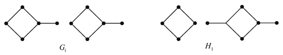
Figure 1. Two generalized co-permanental graphs with 10 vertices and 10 edges.

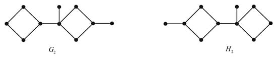
Figure 2. Two generalized co-permanental graphs with 10 vertices and 11 edges.

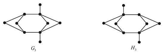
Figure 3. Two generalized co-permanental graphs with 10 vertices and 12 edges.

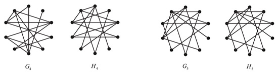
Figure 4. Two pairs of generalized co-permanental graphs with 10 vertices and 14 edges.

4. Conclusions

This paper is a continuance of the research relating to the search of almost-complete graph invariants. In order to find an almost-complete graph invariant, we introduce the generalized permanental polynomials of graphs. As can be seen, the generalized permanental polynomial is quite efficient in distinguishing graphs (networks). It may serve as a powerful tool for dealing with graph isomorphisms. We also obtain the combinatorial expressions for the first five coefficients of the generalized permanental polynomials of graphs.

References

- Dehmer, M.; Emmert-Streib, F.; Grabner, M. A computational approach to construct a multivariate complete graph invariant. Inf. Sci. 2014, 260, 200–208. [Google Scholar] [CrossRef]
- Shi, Y.; Dehmer, M.; Li, X.; Gutman, I. Graph Polynomials; CRC Press: Boca Raton, FL, USA, 2017. [Google Scholar]
- Noy, M. Graphs determined by polynomial invariants. Theor. Comput. Sci. 2003, 307, 365–384. [Google Scholar] [CrossRef]
- Dehmer, M.; Moosbrugger, M.; Shi, Y. Encoding structural information uniquely with polynomial-based descriptors by employing the Randić matrix. Appl. Math. Comput. 2015, 268, 164–168. [Google Scholar] [CrossRef]
- Dehmer, M.; Emmert-Streib, F.; Hu, B.; Shi, Y.; Stefu, M.; Tripathi, S. Highly unique network descriptors based on the roots of the permanental polynomial. Inf. Sci. 2017, 408, 176–181. [Google Scholar] [CrossRef]
- Dehmer, M.; Chen, Z.; Emmert-Streib, F.; Shi, Y.; Tripathi, S. Graph measures with high discrimination power revisited: A random polynomial approach. Inf. Sci. 2018, 467, 407–414. [Google Scholar] [CrossRef]
- Balasubramanian, K.; Parthasarathy, K.R. In search of a complete invariant for graphs. In Lecture Notes in Mathematics; Springer: Berlin/Heidelberg, Germany, 1981; Volume 885, pp. 42–59. [Google Scholar]
- Parthasarathy, K.R. Graph characterising polynomials. Discret. Math. 1999, 206, 171–178. [Google Scholar] [CrossRef]
- Liu, S. On the bivariate permanent polynomials of graphs. Linear Algebra Appl. 2017, 529, 148–163. [Google Scholar] [CrossRef]
- Valiant, L.G. The complexity of computing the permanent. Theor. Comput. Sci. 1979, 8, 189–201. [Google Scholar] [CrossRef]
- Merris, R.; Rebman, K.R.; Watkins, W. Permanental polynomials of graphs. Linear Algebra Appl. 1981, 38, 273–288. [Google Scholar] [CrossRef]
- Kasum, D.; Trinajstić, N.; Gutman, I. Chemical graph theory. III. On permanental polynomial. Croat. Chem. Acta 1981, 54, 321–328. [Google Scholar]
- Cash, G.G. Permanental polynomials of smaller fullerenes. J. Chem. Inf. Comput. Sci. 2000, 40, 1207–1209. [Google Scholar] [CrossRef]
- Tong, H.; Liang, H.; Bai, F. Permanental polynomials of the larger fullerenes. MATCH Commun. Math. Comput. Chem. 2006, 56, 141–152. [Google Scholar]
- Liu, S.; Zhang, H. On the characterizing properties of the permanental polynomials of graphs. Linear Algebra Appl. 2013, 438, 157–172. [Google Scholar] [CrossRef]
- Liu, S.; Zhang, H. Characterizing properties of permanental polynomials of lollipop graphs. Linear Multilinear Algebra 2014, 62, 419–444. [Google Scholar] [CrossRef]
- Wu, T.; Zhang, H. Per-spectral characterization of graphs with extremal per-nullity. Linear Algebra Appl. 2015, 484, 13–26. [Google Scholar] [CrossRef]
- Wu, T.; Zhang, H. Per-spectral and adjacency spectral characterizations of a complete graph removing six edges. Discret. Appl. Math. 2016, 203, 158–170. [Google Scholar] [CrossRef]
- Zhang, H.; Wu, T.; Lai, H. Per-spectral characterizations of some edge-deleted subgraphs of a complete graph. Linear Multilinear Algebra 2015, 63, 397–410. [Google Scholar] [CrossRef]
- Faria, I. Permanental roots and the star degree of a graph. Linear Algebra Appl. 1985, 64, 255–265. [Google Scholar] [CrossRef]
- Li, W.; Liu, S.; Wu, T.; Zhang, H. On the permanental polynomials of graphs. In Graph Polynomials; Shi, Y., Dehmer, M., Li, X., Gutman, I., Eds.; CRC Press: Boca Raton, FL, USA, 2017; pp. 101–122. [Google Scholar]
- Gutman, I. Relation between the Laplacian and the ordinary characteristic polynomial. MATCH Commun. Math. Comput. Chem. 2003, 47, 133–140. [Google Scholar]
- McKay, B.D.; Piperno, A. Practical graph isomorphism, II. J. Symb. Comput. 2014, 60, 94–112. [Google Scholar] [CrossRef]
- Van Dam, E.R.; Haemers, W.H.; Koolen, J.H. Cospectral graphs and the generalized adjacency matrix. Linear Algebra Appl. 2007, 423, 33–41. [Google Scholar] [CrossRef]
© 2019 by the author. Licensee MDPI, Basel, Switzerland. This article is an open access article distributed under the terms and conditions of the Creative Commons Attribution (CC BY) license (http://creativecommons.org/licenses/by/4.0/).