Improving Accuracy of the Kalman Filter Algorithm in Dynamic Conditions Using ANN-Based Learning Module

Abstract

Prediction algorithms enable computers to learn from historical data in order to make accurate decisions about an uncertain future to maximize expected benefit or avoid potential loss. Conventional prediction algorithms are usually based on a trained model, which is learned from historical data. However, the problem with such prediction algorithms is their inability to adapt to dynamic scenarios and changing conditions. This paper presents a novel learning to prediction model to improve the performance of prediction algorithms under dynamic conditions. In the proposed model, a learning module is attached to the prediction algorithm, which acts as a supervisor to monitor and improve the performance of the prediction algorithm continuously by analyzing its output and considering external factors that may have an influence on its performance. To evaluate the effectiveness of the proposed learning to prediction model, we have developed the artificial neural network (ANN)-based learning module to improve the prediction accuracy of the Kalman filter algorithm as a case study. For experimental analysis, we consider a scenario where the Kalman filter algorithm is used to predict actual temperature from noisy sensor readings. the Kalman filter algorithm uses fixed process error covariance R, which is not suitable for dynamic situations where the error in sensor readings varies due to some external factors. In this study, we assume variable error in temperature sensor readings due to the changing humidity level. We have developed a learning module based on ANN to estimate the amount of error in current readings and to update R in the Kalman filter accordingly. Through experiments, we observed that the Kalman filter with the learning module performed better (4.41%–11.19%) than the conventional Kalman filter algorithm in terms of the root mean squared error metric.

1. Introduction

All decision-making processes require a clear understanding of future risks and trends. To avoid potential losses due to the wrong estimate of the future, some people tend to delay the decision as much as possible so that the situation becomes clear in order to make any decision [1]. However, delaying the decision is never a good idea in today’s competitive environment. Human experts can manually process small data, but fail to extract useful information from the humongous data generated and collected in modern information and communications technology-based solutions. Machines can quickly process a large amount of data, but they lack intelligence. As a result, many prediction algorithms have been proposed in the literature to extract the pattern from historical data in order to support intelligent decision-making [2]. Recent advances in computation, communications, and machine learning technologies have transformed almost every aspect of human life through smart solutions. These systems can make use of the knowledge extracted from current and historical data for better decisions in advance to maximize profits or avoid losses [3].

Today, almost all scientific disciplines need to use prediction algorithms in one way or another [4]. Recently, the study of machine learning algorithms has grown enormously due to the considerable progress made in the information storage and processing capabilities of computers. Machine learning algorithms can be broadly classified into four categories: (a) supervised learning, (b) unsupervised learning, (c) semi-supervised learning, and (d) reinforcement learning [5]. Supervised machine learning algorithms make use of labeled data to train the prediction model. The trained prediction model captures the hidden relationship between the input and output parameters, which is then used to estimate the outcome for any given input data, including previously-unseen and -unknown conditions. Numerous prediction algorithms have been proposed in the literature, such as the kth nearest neighbor algorithm (KNN) [6], support vector machines [7], decision trees and random forest [8], neural networks [9], etc. Most of these prediction algorithms are first trained using historical data. After training, the prediction model is fixed and used in the designated application environment. However, the problem with such prediction algorithms is their inability to adapt to the dynamic scenarios and changing conditions.

There are several well-known ensemble approaches for prediction and classification problems, such as ensembles, stacked generalization, a mixture-of-experts, etc. The combination of more than one network to solve a problem is called an ensemble neural network. The performance of the ensemble neural network is better compared to the individual neural network due to the numerous errors of different neural networks [10]. Stacked generalization is another ensemble approach in which numerous prediction algorithms are combined into one. The stacked generalization method provides good results compared to the single-neural network method [11]. The mixture-of-experts is also a very famous method, which is based on many statistical estimation methods that were developed to improve the prediction accuracy [12].

Enabling prediction algorithms to cope with dynamic data or changing environmental conditions is a challenging task. In this paper, we propose a general architecture to improve the performance of the prediction algorithm using the learning module. The learning module continuously monitors the performance of the prediction algorithm by receiving its output as feedback. The learning module may also consider the external parameters that may have an influence on the performance of the prediction algorithm. After analyzing the current external factors and the output of the prediction algorithm, the learning module updates the tunable parameters or swaps the trained model of the prediction algorithm to improve its performance in terms of prediction accuracy. For experimental analysis, we have used the Kalman filter as a prediction algorithm, and our learning module is based on artificial neural networks.

The rest of the paper is organized as follows: A brief overview of related work is presented in Section 2. In Section 3, we present the conceptual design of the proposed learning to prediction model with a detailed description of the selected case study. A detailed discussion of the experimental setup, implementations, and performance analysis is presented in Section 4. Finally, we conclude this paper in Section 5 with an outlook toward our future work.

2. Related Work

Recently, tremendous growth and improvement have been experienced in the processing and storage capabilities of computing devices. Computer programs can quickly process a huge amount of data to extract patterns and other information. As a result, the study of machine learning algorithms has grown enormously due to the considerable progress made in the information storage and processing capabilities of computers. Prediction algorithms are actively used in many different applications in diverse domains, e.g., stock market predictions, customer prediction, energy prediction, risk prediction, weather prediction, etc. Numerous prediction algorithms have been proposed in the literature. The kth nearest neighbor algorithm (KNN) is a simple and useful algorithm commonly used for both regression and classification problems [13,14]. The KNN algorithm predicts the outcome for a new data instance based on the majority votes among the kinstances in its neighborhood. The neighborhood is computed using various distance functions, e.g., Manhattan, Hamming, Euclidean, etc. Support vector machines (SVM) and their variants form another class of prediction algorithms that attempt to find the optimal line/plane/hyperplane in the multidimensional space that should be at the furthest distance from each class in the dataset [15]. Often, it is very difficult to express or interpret the knowledge captured by the prediction algorithm from training data in a human-readable format. To this end, decision tree algorithms provide clear and explicit rules that are extracted by the algorithm in a human-readable format [16]. There are many variants of decision tree algorithms, and the most popular are classification and regression trees (CART) [17], iterative dichotomizer 3 (ID3) [18], the C4.5 algorithm [19], and chi-squared automatic interaction detector (CHAID) [20]. Mridula et al. presented a very brief comparative analysis of these variants in [21]. Today, the classification and regression tree has grasped the attention of many researchers and has been used numerous times in different areas for prediction purposes. The CART has the capability to solve the complicated interrelation between predictive parameters, which cannot be solved by using conventional multivariate algorithms. The CART is a machine learning technique that is commonly used to construct prediction models from the data. The CART model is constructed of mainly two trees, namely classification trees and regression trees, which are designed for dependent variables without order and with order, respectively. The calculation of the prediction error is carried out by the squared difference between the observed and predicted values. Instead of using a single decision tree, the random forest algorithm further extends the concept by generating several decision trees through random sampling over the feature subset [22], thus avoiding the over-fitting issues. In supervised learning, prediction algorithms are first trained using historical data. After training, the prediction model is fixed and used in the designated application environment. However, the problem with such prediction algorithms is their inability to adapt to dynamic scenarios and changing conditions.

The artificial neural network (ANN) is considered among the most powerful nature-inspired prediction algorithms, which mimics the working neurons in human brain [23]. ANN algorithms are general-purpose learning algorithms and are actively used in solving a wide range of problems including regression, classification, clustering, pattern recognition, forecasting, and time series data processing [24,25,26,27]. The functionality of the neuron is modeled inside the perceptron, which is an atomic functional unit of ANN. Operation inside the perceptron includes multiplication of inputs with corresponding weights, summation of the results with a bias, and output generation using an activation function such as sigmoid. Depending on the problem size and nature, the appropriate number of perceptrons is connected in a layered fashion (input layer, hidden layer, output layer) to form an artificial neural network (ANN) architecture. Learning in ANN algorithms is all about the weight adjustment of perceptrons in the network, which is accomplished in a systematic fashion using different methods, e.g., error back-propagation, gradient calculation methods [28], etc. Conventional ANN algorithms require input pre-processing, normalization and feature extraction, which essentially dictate their performance and accuracy. Furthermore, ANN network design is more of an art than a science, and trial-and-error methods are most commonly used to decide the number of layers in the network, the number of neurons in each layer, the activation function, and the connectivity among the layers. Previously, the ANN network’s size was mainly restricted due the limited computational power. However, with the advent of modern high-speed multicore processors, we can virtually have an ANN network of any size, and this has led to the emergence of a whole new field under the umbrella of neural networks, i.e., deep learning or deep neural networks. Machine learning has gained remarkable attention recently due to significant results produced by deep learning algorithms such as recurrent neural networks (RNN), convolution neural networks (CNN), long short-term memory (LSTM), etc. [29,30,31,32]. More recent high-performance prediction algorithms based on deep learning architectures (such as CNN, RNN, LSTM) are focused on the elimination of pre-processing and feature extraction in complex problem solving instead of adaptation with the dynamic conditions.

The adaptive neuro-fuzzy inference system (ANFIS) is a feed-forward neural network having many layers [33]. The neural network algorithms and fuzzy reasoning are used for training and mapping inputs to outputs, respectively. ANFIS has the potential to integrate the linguistic power of a fuzzy inference system and the numeric power of a neural network. The central advantage of ANFIS is that it allows the extraction of fuzzy rules from numerical data or expert knowledge. The main disadvantage of ANFIS is that it takes more processing time due to the structure training and parameter determination. ANFIS has been actively used in different areas for different purposes, e.g., diagnosis, wind speed prediction, forecasting, etc. Zhou et al. proposed a method in which the assessment of the ensemble neural networks was carried out for both regression and classification problems [10]. The results illustrate that it was better to ensemble some of the neural networks rather than all the neural networks. A solution named genetic algorithm-based selective ensemble neural networks (GASEN) was proposed in order to select neural networks for ensembles based on some evolved weights. The comparison of the GASEN model with some famous ensemble methods such as bagging and boosting was carried out, but the GASEN outperformed these algorithms. Wolpert et al. proposed a method named stacked generalization in which the different predictive algorithms are combined in order to improve the predictive accuracy [11]. Breiman et al. carried out a demonstration of how how stacking can be used for predictive accuracy in the context of regression [34]. The results indicated that by using the stacking method, the predictive performance was improved. Jacobs et al. suggested another approach named the mixture-of-experts with the goal that the combination of many statistical estimates would increase the predictive accuracy as compared to a single estimate [35].

Prediction algorithms belonging to the family of reinforcement learning allow the algorithm to improve its performance based on the reward it receives on the basis of its previous outcome. These algorithms are commonly used in game theory, control theory, and multi-agent-based applications [36,37]. Each time the algorithm generates the output, it receives a reward (positive or negative) depending on the difference between the produced and desired outcome. Thus, the algorithm learns from its experience and tries to maximize the positive rewards and avoid negative rewards. These algorithms are useful where learning is only possible through interaction with the environment. These algorithms continuously improve their performance and finally converge. After convergence, the algorithms rarely change their behavior with changing environmental conditions. In other words, a single trained model restricts the reinforcement learning algorithm to adapt to the dynamic conditions.

Enabling the prediction algorithm’s adaptation with dynamically-changing environmental conditions requires a mechanism that can somehow detect the occurrence of environmental changes and then make necessary changes in the prediction algorithm to avoid performance degradation. This approach can be realized by integrating a learning module with the prediction algorithm to continuously tune its performance. Some studies closely related to this concept can be found in the literature; for instance, Kang et al. developed a fuzzy inference-based system to tune the performance of the Kalman filter algorithm for accurate attitude estimation of a humanoid robot [38]. In static conditions, the Kalman filter can successfully remove noise from gyro sensors’ readings to predict the accurate orientation of the robot. However, when the robot is moving, the gyro sensors’ readings become noisy. To resolve this issue, they have used accelerometers sensors to detect the robot’s current state, and Kalman filter algorithm was accordingly tuned using the fuzzy algorithm. Likewise, Ibarra et al. proposed an adaptive neuro-fuzzy inference (ANFIS)-based system to tune the Kalman filter algorithm for accurate attitude estimation based on the gyroscope and accelerometer sensors [39], while others used hidden Markov models (HMM) for the same purpose [40].

With the passage of time, researchers have made some modifications of the Kalman filter with the goal to improve its performance. Among such attempts is included the extended Kalman filter, which is the nonlinear form of the basic Kalman filter. The extended Kalman filter linearizes the estimate of the current mean and covariance. The iterated extended Kalman filter is another version of the Kalman filter, which calculates the state estimates as a maximum posterior estimate. The extended Kalman filter is an iterated Kalman filter method with one iteration where the update is performed using the Gauss–Newton technique [41]. The ensemble Kalman filter is another version of the Kalman filter with a recursive filter, appropriate in a situation where a greater number of parameters needs to be taken into account. The extended and particle filter have the same characteristics, the only difference being that the ensemble Kalman filter makes the supposition that all the probabilities involved are Gaussian [42,43]. The Kalman filter is also fused with some other methods such as the unbiased finite-impulse response (UFIR) filter. The fusion filter is robust, but does not provide optimal results. The fusion filter combines both the Kalman filter and UFIR, which decreases the error [44]. It is also very useful to blend the machine learning algorithms with other methods to enable the decision support system to make correct decisions. A solution named the adaptive artificial neural network has been proposed for this purpose to make the computation more precise [45].

The proposed learning to prediction model presented in this paper is a generalized model that can be used to tune the performance of any prediction algorithm under dynamic conditions. In contrast to the single trained model in conventional prediction algorithms, the proposed learning to prediction model is focused on the learning and maintenance of various training models at the same time, which are learned by the learning module. Each trained model suits a particular environmental condition and shall be activated through the updating of the tunable parameters or complete replacement of the trained model in prediction algorithm when environmental triggers are observed.

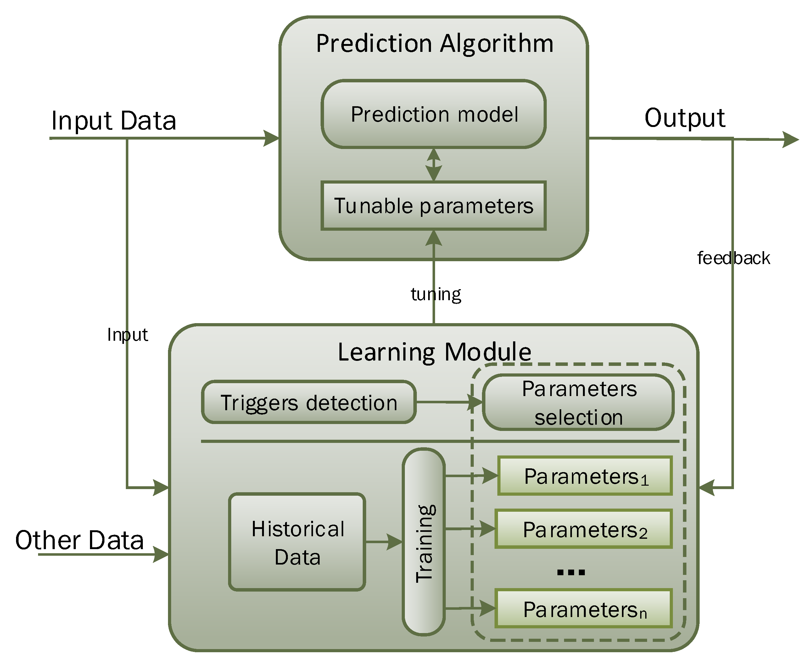
3. Proposed Learning to Prediction Scheme

Conventionally, prediction algorithms are first trained using historical data, so that they can learn the hidden pattern and relationship among input and output parameters. Afterwards, trained models are used to predict the output for any given input data. The prediction algorithm will perform well when input data and the application scenario remain the same as the training data conditions. However, the existing prediction algorithm does not allow adaptation of the trained model with changing and dynamic input conditions. To overcome this limitation, we propose the learning to prediction model, as shown in Figure 1. The learning module is used to tune the prediction algorithm to improve its performance in terms of prediction accuracy. In the proposed model, the learning module acts like a supervisor that continuously monitors the performance of the prediction algorithm by receiving its output as feedback. The learning module may also consider the external parameters that may have an influence on the performance of the prediction algorithm. After analyzing the current external factors and output of the prediction algorithm, the learning module may update the tunable parameters of the prediction algorithm or completely replace the trained model in prediction algorithm to improve its performance in terms of prediction accuracy when environmental triggers are observed.

Figure 1. Conceptual view of the proposed learning to prediction model.

For the experimental analysis, we have used the Kalman filter as the prediction algorithm, and our learning module is based on artificial neural networks, as shown in Figure 2. The Kalman filter is a lightweight algorithm that does not require all historical data, but only previous state information to make an intelligent prediction about the actual state of the system [46,47]. In this study, the Kalman filter algorithm is used to predict actual temperature from noisy temperature sensor readings. Noise in temperature sensor readings is introduced based on a scenario where temperature sensor readings are heavily influenced by the surrounding humidity level. For the learning module, we choose to use the artificial neural network (ANN) algorithm, which takes three input parameters, i.e., current temperature, predicted temperature (feedback), and humidity level. The Kalman filter algorithm gets readings from the temperature sensor at time t, i.e., $z_t$, and will predict actual temperature $T_t$ by removing noise. The Kalman filter algorithm’s performance is mainly controlled through a tunable parameter known as Kalman gain (K), which is updated after every iteration using the process covariance matrix (P) and the estimated error in sensors readings (R). The learning module will try to find the estimated error in sensors’ readings (R), so that K can be updated intelligently. Before going into the detailed architecture, we present a brief description of the Kalman filter algorithm in the next sub-section.

Figure 2. Block diagram for temperature prediction using ANN-based learning with the Kalman filter.

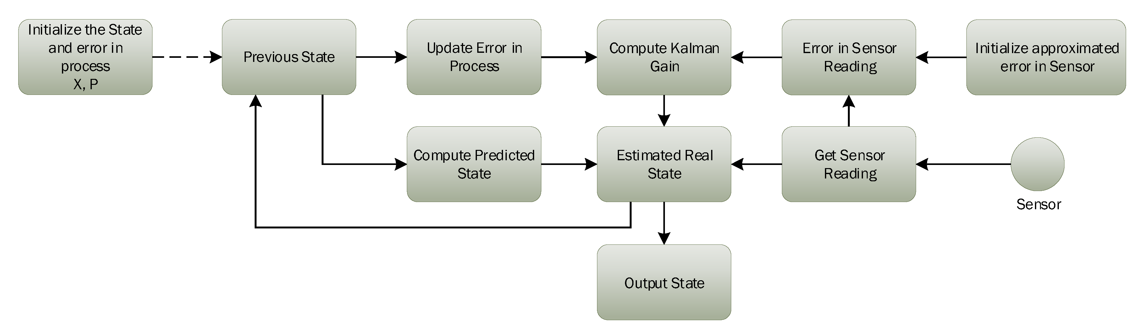
3.1. Kalman Filter Algorithm

Kalman’s filter is a lightweight algorithm that does not require all historical data, but only previous state information to make an intelligent prediction about the actual state of the system. Kalman gain K is one of the most important parameters of the Kalman filter’s design, which performs all the magic. Kalman filter algorithm updates the value of K depending on the situation to control weights given to the system’s own predicted state or sensor readings. Figure 3 presents the essential components and working of the Kalman filter algorithm.

Figure 3. Working of the Kalman filter algorithm.

Every environment has its noise factors, which can seriously affect sensor readings in that environment. In this study, we consider a temperature sensor reading having noise, and let us assume $T_t$ is the temperature at time t. The Kalman filter algorithm includes the process model that can make an internal prediction about the system state, i.e., estimated temperature, and then, it is compared with current sensor readings to decide predicted temperature $T_{t+1}$ at time $t+1$. Next, we briefly explain the step-by-step working of that Kalman filter algorithm, that is how it removes the noise from sensor data.

In the first step, the predicted temperature is computed from the previously-estimated value using the formula given below.

$$T_p=A·T_{t-1}+B·u_t$$

(1)

where $T_p$ is internally-predicted temperature, A and B represent the state transition and control matrices, respectively. $T_{t-1}$ is the temperature at time $t-1$, i.e., previously calculated, and $u_t$ represents the control vector.

Uncertainty in the internally-predicted temperature is determined by a covariance factor, which is updated using the following formula.

$$P_{predicted}=A·P_{t-1}·A^T+Q$$

(2)

where A and $A^T$ represent the state transition matrix and its transpose, and the old value of covariance is $P_{t-1}$ along with an estimated error in the process represented by Q.

After making an internal estimate about system next state and updating covariance, Kalman’s gain K is updated as follows.

$$K=\frac{P_{predicted}·H^T}{H·P_{predicted}·H^T+R}$$

(3)

where H and $H^T$ represent the observation matrix and its transpose, whereas the estimated error in the measurements is expressed as R.

Let us assume that current reading obtained from the temperature sensor at time t is represented as $z_t$. Then, the predicted temperature given by Kalman’s filter is calculated using the following equation.

$$T_t=T_{predicted}+K(z_t-H·T_{predicted})$$

(4)

In the final step, the covariance factor is updated for the next iteration as below:

$$P_t=(I-K·H)P_{predicted}$$

(5)

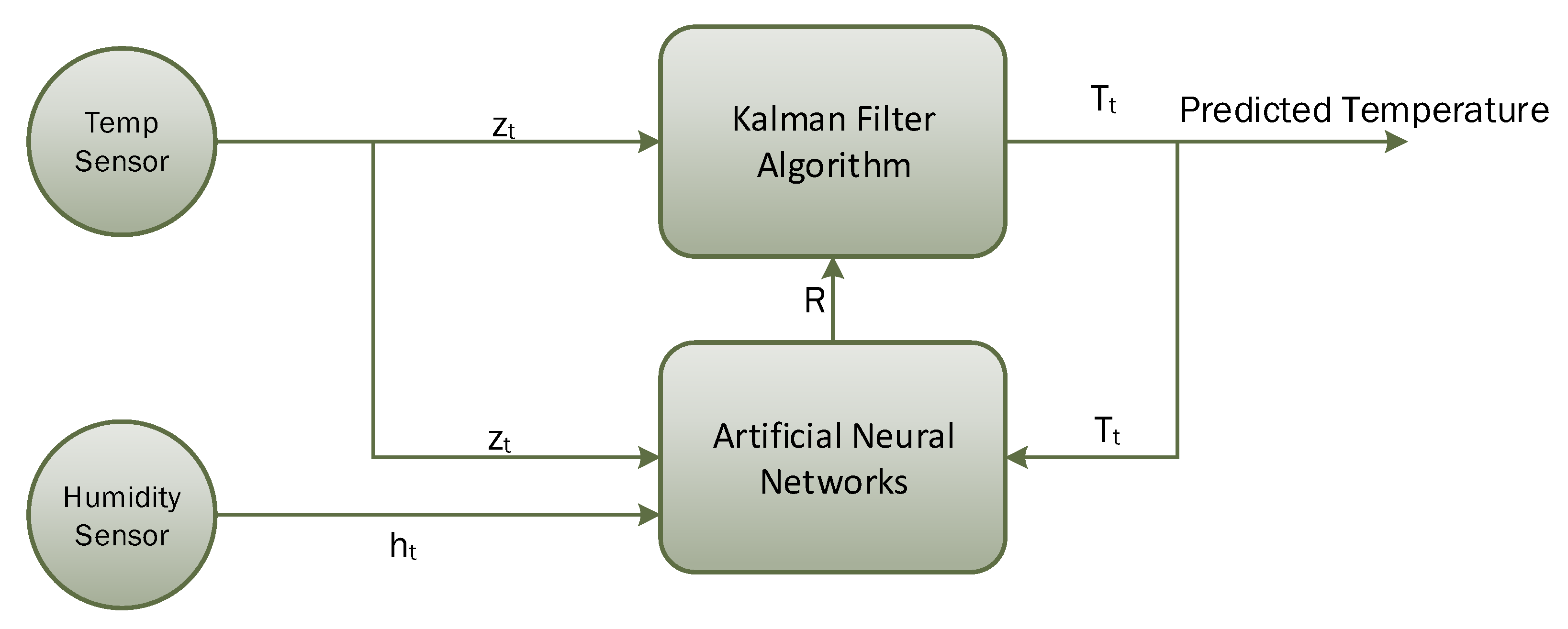
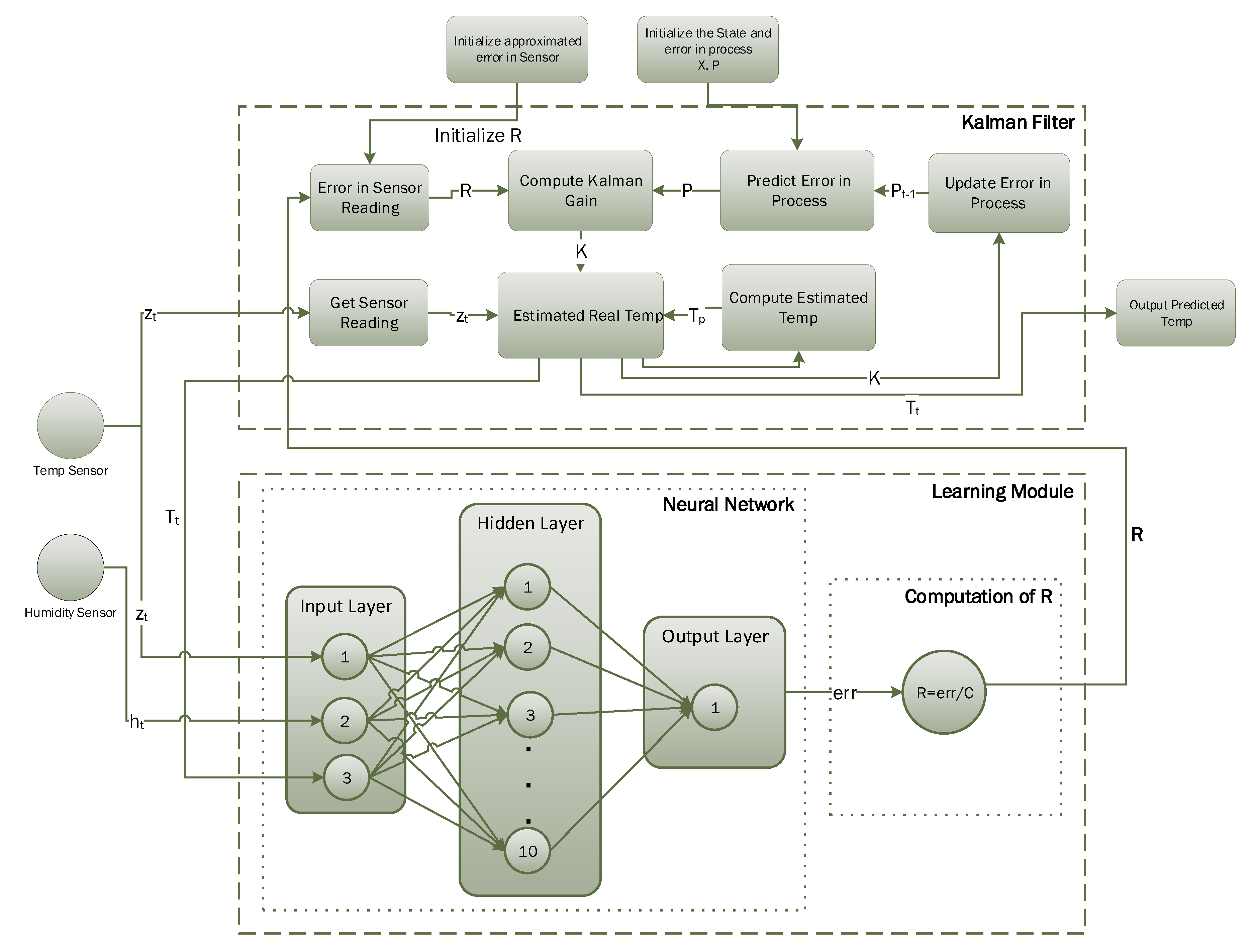
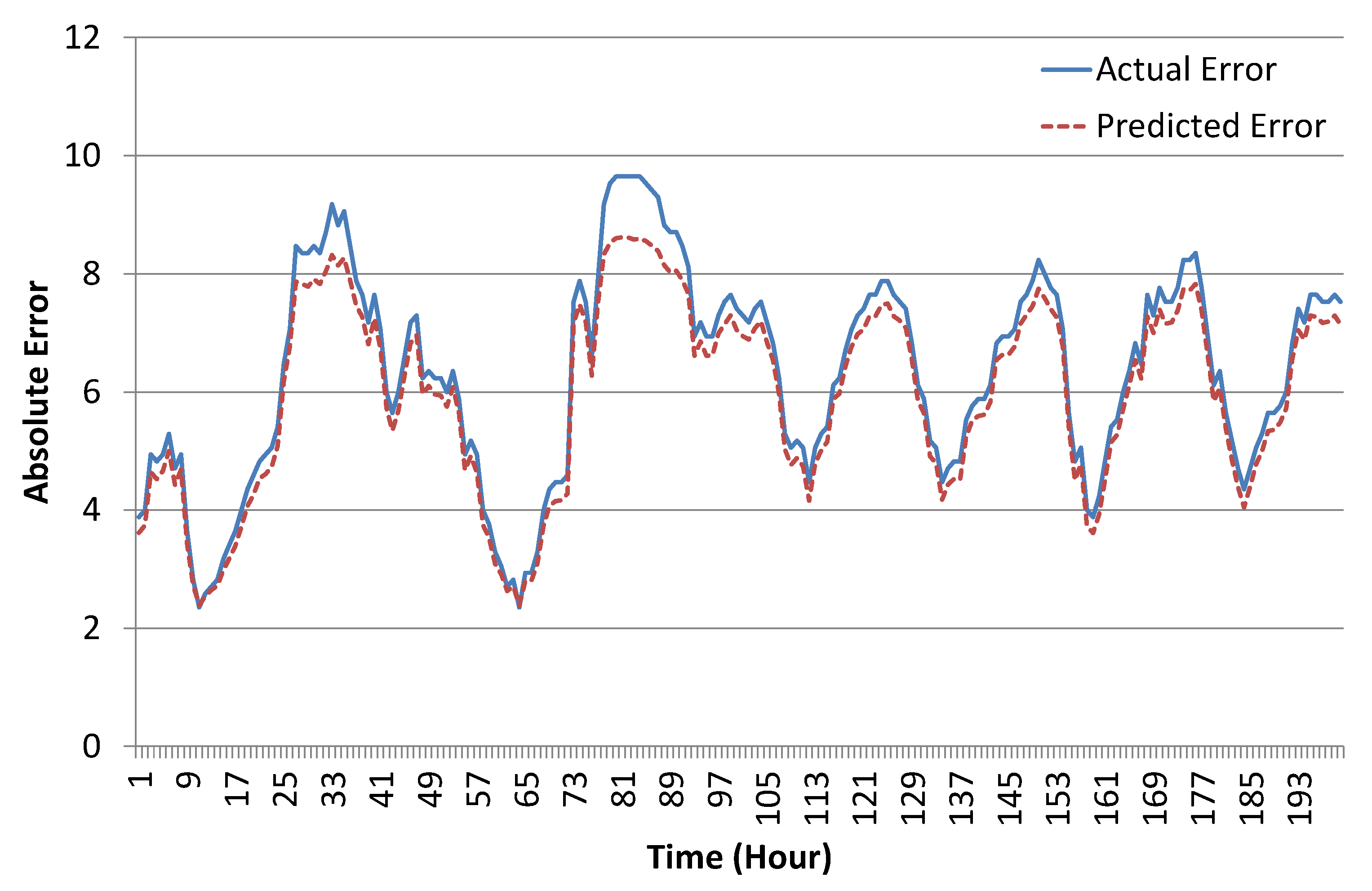
3.2. ANN-Based Learning to Prediction for the Kalman Filter

Figure 3 presents the flow diagram illustrating the operation of the Kalman filter, which works fine when the estimated error in the sensor is not changing. However, if error in the sensor reading changes due to some other (external) parameter, then we need to update estimated error in the measurements (R), accordingly. In this study, we consider a scenario where temperature sensor readings are affected by humidity level. A random amount of error is introduced in sensor readings based on the current humidity level using a uniform distribution. The conventional Kalman filter algorithm fails to predict actual temperature under these dynamic conditions. Figure 4 presents the detailed working diagram of the proposed learning to prediction scheme. The learning module is based on an artificial neural network algorithm taking three inputs, i.e., current temperature, current humidity, and previously-predicted temperature by the Kalman filter algorithm. The output of the ANN algorithm is the predicted error in sensor readings, which is then divided by a constant factor (F) to compute the estimated error in sensor readings, i.e., R. The updated value of R is then passed to the Kalman filter algorithm to tune its prediction accuracy by appropriately adjusting the Kalman gain (K). The proposed learning to prediction model enables the Kalman filter to estimate the actual temperature accurately from noisy sensor readings with a dynamic error rate.

Figure 4. Detailed diagram for temperature prediction using the Kalman filter with the learning module.

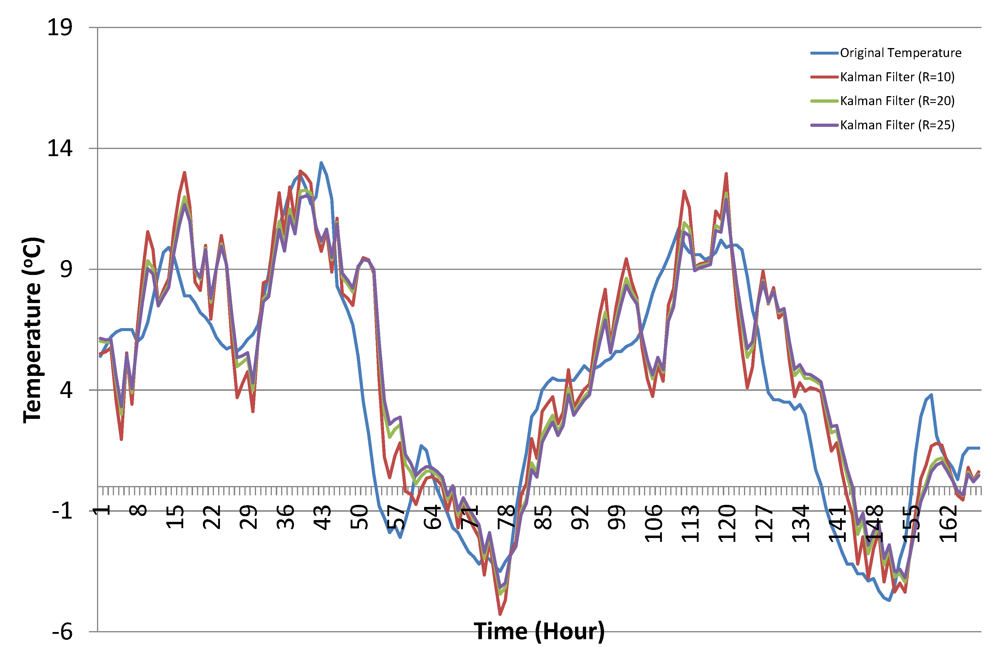
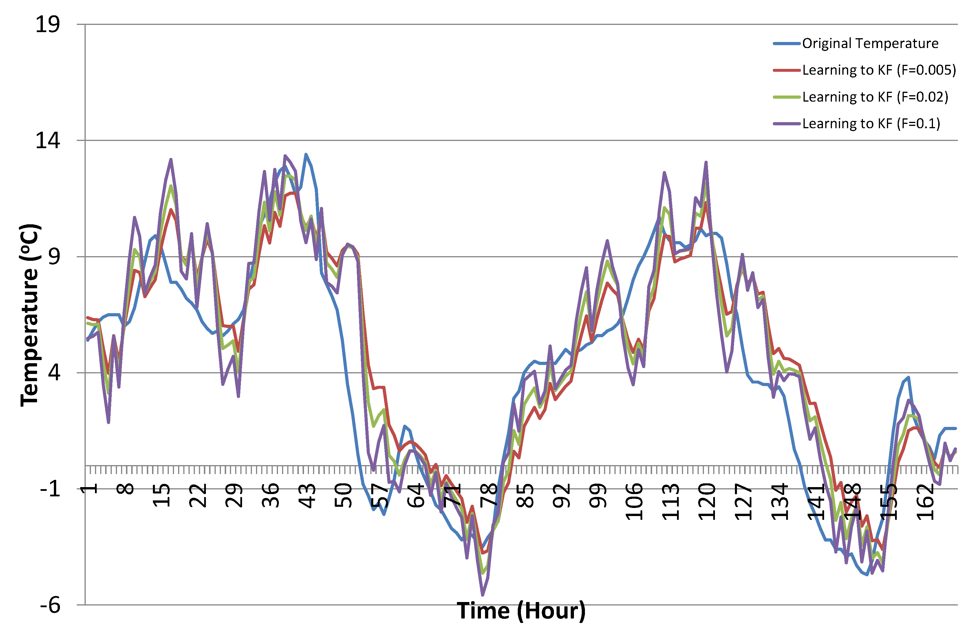
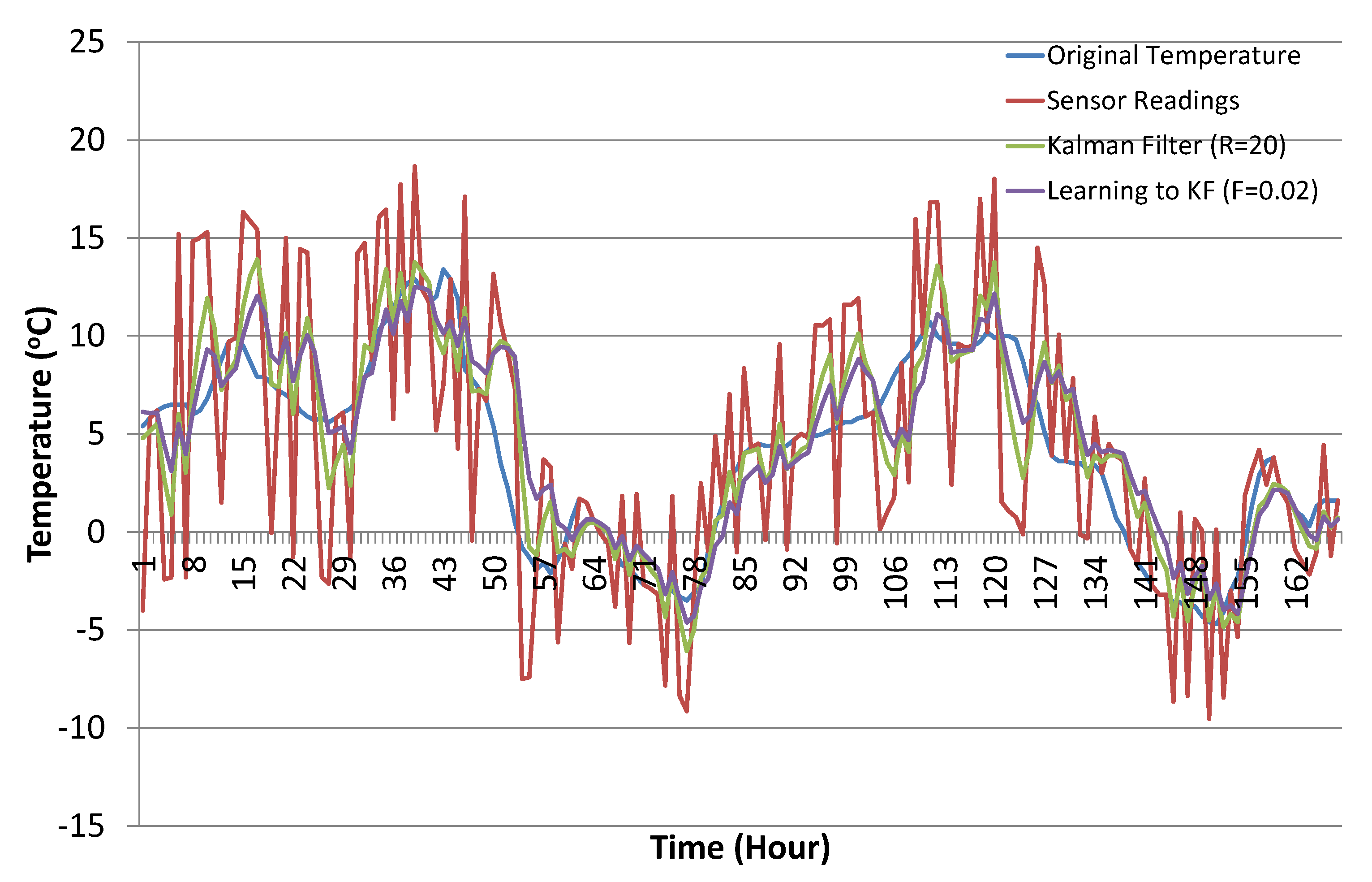
4. Experimental Results and Discussion

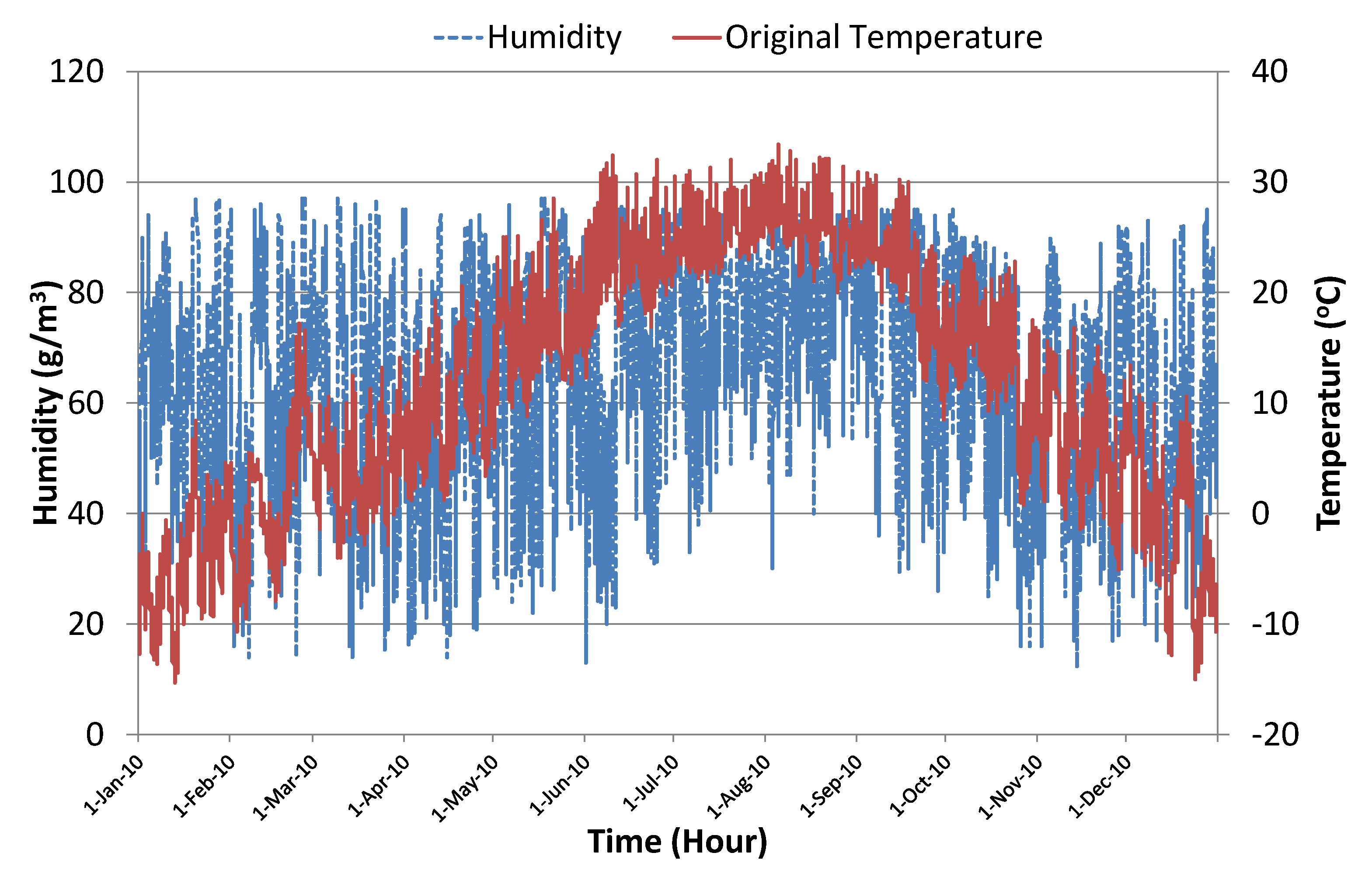
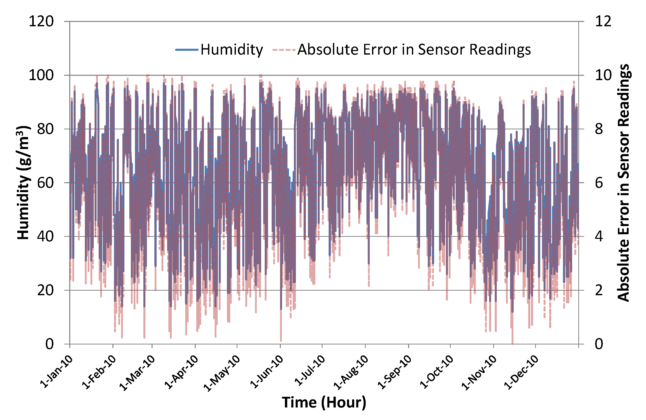
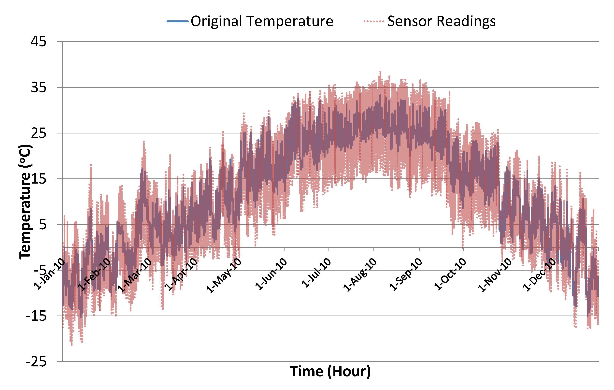
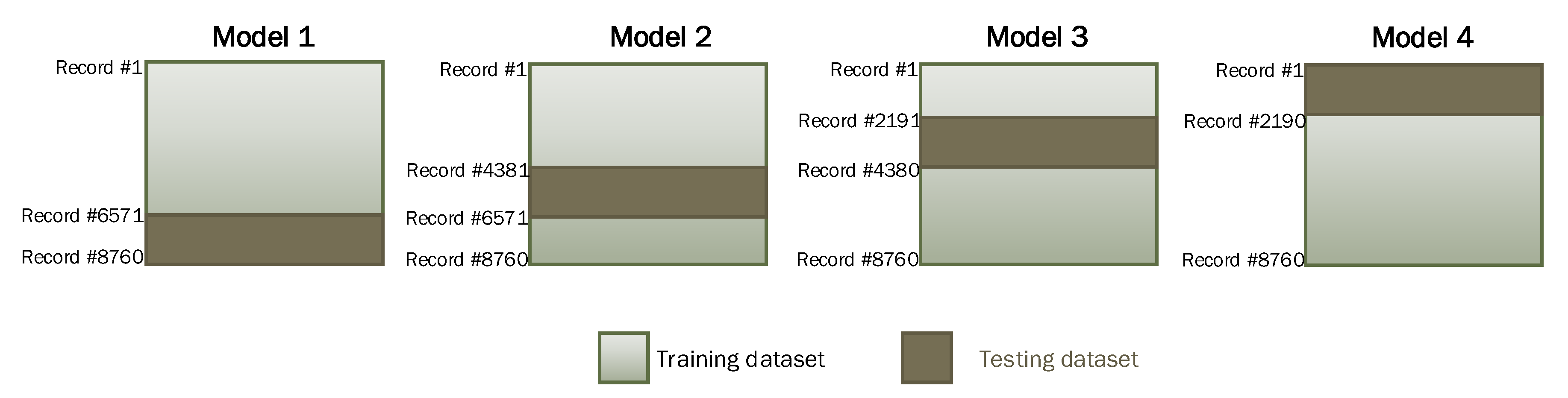
4.1. Experimental Setup

For the experimental analysis, we used real data of temperature and humidity level collected for a one-year period in Seoul, South Korea. Figure 5 shows the actual values of temperature and humidity data collected over an hourly interval from 1 January–31 December 2010. There was in total $365\times 24=8760$ data instances. To find the correlation between actual temperature and humidity level, we used the Pearson correlation coefficient formula given below.

$$Correl(T,H)=\rho =\frac{\sum (t_i-\overline{t})(h_i-\overline{h})}{\sqrt{\sum {(t_i-\overline{t})}^2\sum {(h_i-\overline{h})}^2}}$$

(6)

where $Correl(T,H)$ is the correlation coefficient $\rho$ between temperature and humidity and $t_i$ and $h_i$ represent the temperature and humidity values in the ith hour, respectively. The mean values of temperature and humidity are expressed as $\overline{t}$ and $\overline{h}$, respectively.

Figure 5. Temperature and humidity data.

There exists a significant, but weak, positive correlation between humidity level and the actual temperature, $r\left(8758\right)=0.22$, $p<0.0001$. To create dynamically-changing conditions, we introduced error into the temperature sensor readings based on the humidity level using a uniform distribution. The amount of error was randomly generated, but it was proportional to the normalized current humidity level, i.e.,

$$\left|Err\right|\propto \frac{h_{cur}-h_{\mathit{min}}}{h_{\mathit{max}}-h_{\mathit{min}}}$$

(7)

where $\left|Err\right|$ is the absolute error in temperature sensor readings and $h_{cur}$, $h_{\mathit{max}}$, and $h_{\mathit{min}}$ represent the current humidity level, maximum humidity level, and minimum humidity level, respectively. To compute the simulated sensor readings with noise, we have used the following formula.

$$T_{sen}=\frac{h_{cur}-h_{\mathit{min}}}{h_{\mathit{max}}-h_{\mathit{min}}}\times \Re (-1,1)\times S+T_{org}$$

(8)

where $T_{sen}$ is the simulated sensor reading with noise, ℜ is used to generate a random number between −1 and +1 using a uniform distribution, S is used for the scaling factor of the error, and $T_{org}$ is the original (actual) temperature.

Figure 6 shows the actual humidity level along with the corresponding randomly-generated error in temperature sensor readings. To introduce sufficient noise to generate dynamic conditions, we used scaling factor $S=10$ in these experiments. This was good enough to significantly disturb the Kalman filter algorithm’s prediction accuracy, thus creating a test scenario for the evaluation of the proposed learning to prediction model. Figure 7 shows the actual temperature values along with simulated sensor readings with randomly-generated noise using scaling factor $S=10$. Table 1 presents a brief summary of the collected data and simulated noisy sensor data.

Figure 6. Humidity and absolute error in sensor readings.

Figure 7. Original temperature and simulated noisy sensor readings’ data.

Table 1. Summary of collected and simulated noisy data.

Measure	Temperature (${}^{\circ }$C)	Temperature Sensor Readings (${}^{\circ }$C)	Humidity (g/m${}^3$)	Absolute Error in Temperature Sensor Readings
Minimum	−15.30	−21.36	12.00	0.00
Maximum	33.40	38.58	97.00	10.00
Average	12.14	12.16	62.90	5.99
Stdev	11.39	12.58	19.89	2.34

4.2. Implementation

We implemented the proposed system for the evaluation of the Kalman filter algorithm with the learning module in Visual C#. The experiments were performed on a real dataset containing temperature and humidity data for a one-year duration along with simulated noisy sensor readings. We loaded the data from an external text file and stored it inside the application’s data structure. The data contained four input parameters, i.e., original temperature, noisy sensor reading, humidity level, and amount of error. First, we computed the root mean squared error (RMSE) for sensor readings by comparing its values with the original temperature data. The RMSE for sensor readings is very high, i.e., 5.21.

Next, we used the Kalman filter algorithm to predict actual temperature from the noisy sensor reading. The implementation interface provides manual tuning of the Kalman filter internal parameter, i.e., estimated error in measurement (R). Experiments were conducted with different values of R, and the corresponding results were collected. The RMSE for predicted temperature using the Kalman filter with $R=20$ was 2.49, which was much better than the RMSE of sensor readings, i.e., $52.20\%$ reduction of the error. However, it still needs improvement. We have used the Accord.NET framework [48] for the implementation of the ANN-based learning module to predict and tune the error rate in measurement to improve the prediction accuracy of the Kalman filter algorithm. The ANN algorithm has three neurons in the input layer for humidity data, sensing, and predicted temperature data and one neuron in the output layer for predicting the error in sensor readings. Input and output data were normalized using the following equation.

$$\widetilde{d_i}=\frac{d_i-d_{\mathit{min}}}{d_{\mathit{max}}-d_{\mathit{min}}}$$

(9)

where $\widetilde{d_i}$ is the normalized value for the ith data point of the input and output parameters, i.e., humidity, sensing, and predicted temperature, and the predicted error in sensor readings. $d_{\mathit{min}}$ and $d_{\mathit{max}}$ are the corresponding minimum and maximum values in the available dataset for each parameter.

As the ANN network is trained with normalized data, therefore, we need to de-normalize the output of the neural network to get the corresponding predicted error using the following equation.

$$er{r}_i=\widetilde{er{r}_i}\times (er{r}_{\mathit{max}}-er{r}_{\mathit{min}})+er{r}_{\mathit{min}}$$

(10)

For ANN algorithm training, different configurations were considered by changing the number of neurons in the hidden layer, the activation function, and learning rates. For every configuration of ANN, multiple independent experiments were conducted for training, and average results are reported to factor out the stochastic element in ANN network weights’ initialization. Furthermore, to avoid bias in the training process, the 4-fold cross-validation technique was used for every configuration in all experiments. For this purpose, we divided the dataset into four subsets of equal size (i.e., 2190 instances in each subset). Figure 8 illustrates the training and testing dataset used for each model in our 4-fold cross-validation process. As per this scheme, $75\%$ of the data were used for training, and the remaining $25\%$ was used for testing the ANN algorithm with the selected configuration in each experiment. Table 2 provides detailed information regarding the selected configuration for ANN and the corresponding prediction accuracy in terms of RMSE for training and testing datasets in each model. The ANN training algorithm was based on the Levenberg–Marquardt algorithm, which is considered to be the best and fastest method for moderately-sized neural networks [49]. The maximum number of epochs used to train the ANN network was 100.

Figure 8. Training and testing dataset using the 4-fold cross-validation model.

Table 2. ANN algorithm prediction results in terms of RMSE for training and testing datasets with different configurations using the 4-fold cross-validation model.

ANN Configuration			Experiment ID	Model 1		Model 2		Model 3		Model 4		Models Average (Test Cases)	Experiments Average (Test Cases)
Hidden Layers	Activation Function	Learning Rate		Training	Test	Training	Test	Training	Test	Training	Test
5	Linear	0.1	1	4.45	5.19	5.04	3.18	4.50	5.05	4.56	4.88	4.57
5	Linear	0.1	2	4.45	5.19	5.04	3.18	4.50	5.05	4.56	4.88	4.57
5	Linear	0.1	3	4.45	5.19	5.04	3.18	4.50	5.05	4.56	4.88	4.57	4.57
5	Linear	0.2	1	4.45	5.19	5.04	3.18	4.50	5.05	4.56	4.88	3.28
5	Linear	0.2	2	4.45	5.19	5.04	3.18	4.50	5.05	4.56	4.88	4.57
5	Linear	0.2	3	4.45	5.19	5.04	3.18	4.50	5.05	4.56	4.88	4.57	4.14
5	Sigmoid	0.1	1	0.30	0.28	0.22	0.24	0.22	0.23	0.35	0.35	0.27
5	Sigmoid	0.1	2	0.21	0.18	0.22	0.25	0.22	0.23	0.06	0.09	0.19
5	Sigmoid	0.1	3	0.23	0.21	0.10	0.12	0.15	0.15	0.24	0.27	0.19	0.22
5	Sigmoid	0.2	1	0.16	0.15	0.18	0.18	0.22	0.24	0.22	0.25	0.21
5	Sigmoid	0.2	2	0.22	0.24	0.14	0.18	0.18	0.22	0.19	0.22	0.22
5	Sigmoid	0.2	3	0.11	0.20	0.22	0.23	0.23	0.23	0.24	0.26	0.23	0.22
10	Linear	0.1	1	4.45	5.19	5.04	3.18	4.50	5.05	4.56	4.88	4.57
10	Linear	0.1	2	4.45	5.19	5.04	3.18	4.50	5.05	4.56	4.88	4.57
10	Linear	0.1	3	4.45	5.19	5.04	3.18	4.50	5.05	4.56	4.88	4.57	4.57
10	Linear	0.2	1	4.45	5.19	5.04	3.18	4.50	5.05	4.56	4.88	4.57
10	Linear	0.2	2	4.45	5.19	5.04	3.18	4.50	5.05	4.56	4.88	4.57
10	Linear	0.2	3	4.45	5.19	5.04	3.18	4.50	5.05	4.56	4.88	4.57	4.57
10	Sigmoid	0.1	1	0.24	0.21	0.10	0.10	0.24	0.24	0.21	0.24	0.20
10	Sigmoid	0.1	2	0.26	0.22	0.20	0.22	0.27	0.27	0.52	0.36	0.27
10	Sigmoid	0.1	3	0.28	0.23	0.11	0.13	0.08	0.08	0.31	0.33	0.19	0.22
10	Sigmoid	0.2	1	0.20	0.16	0.09	0.10	0.23	0.25	0.24	0.27	0.19
10	Sigmoid	0.2	2	0.25	0.27	0.20	0.22	0.19	0.20	0.18	0.21	0.22
10	Sigmoid	0.2	3	0.24	0.19	0.15	0.16	0.24	0.24	0.22	0.23	0.21	0.21
15	Linear	0.1	1	4.45	5.19	5.04	3.18	4.50	5.05	4.56	4.88	4.57
15	Linear	0.1	2	4.45	5.19	5.04	3.18	4.50	5.05	4.56	4.88	4.57
15	Linear	0.1	3	4.45	5.19	5.04	3.18	4.50	5.05	4.56	4.88	4.57	4.57
15	Linear	0.2	1	4.45	5.19	5.04	3.18	4.50	5.05	4.56	4.88	4.57
15	Linear	0.2	2	4.45	5.19	5.04	3.18	4.50	5.05	4.56	4.88	4.57
15	Linear	0.2	3	4.45	5.19	5.04	3.18	4.50	5.05	4.56	4.88	4.57	4.57
15	Sigmoid	0.1	1	1.15	0.91	0.27	0.34	0.34	0.33	0.24	0.27	0.46
15	Sigmoid	0.1	2	0.13	0.11	0.23	0.25	0.23	0.20	0.31	0.31	0.21
15	Sigmoid	0.1	3	0.57	0.45	0.34	0.36	0.22	0.22	0.19	0.23	0.31	0.33
15	Sigmoid	0.2	1	0.27	0.23	0.56	0.91	0.19	0.22	0.40	0.40	0.44
15	Sigmoid	0.2	2	0.24	0.20	0.22	0.25	0.26	0.29	0.20	0.23	0.24
15	Sigmoid	0.2	3	0.25	0.19	0.20	0.24	0.21	0.22	0.21	0.24	0.22	0.30

The reported results reveal that with the linear activation function, resulted in ANN being rarely affected by changing the number of neurons in the hidden layer or the learning rate. However, significant variation in prediction accuracy can be observed for each model in the 4-fold cross-validation process. Interestingly, in the case of Model 2, higher prediction accuracy was achieved with the testing dataset as compared to the training dataset. The sigmoid activation function is commonly used in the ANN algorithm, and significant improvement in the prediction accuracy can be observed in the reported results in comparison to the linear activation function. The best case results (highlighted in bold) were achieved for the ANN algorithm with the sigmoid activation function having 10 neurons in the hidden layer with a learning rate of 0.2. The same configuration is further used for tuning the performance of the Kalman filter algorithm.

The screenshot given in Figure 9 shows the learning accuracy of the ANN algorithm with the best configuration for 200 sample data instances. The ANN predicted error rate was well aligned with the original error rate in data, which shows that our learning module was perfectly trained on the given data-set. As stated earlier, R is the estimated error in measurements, which is directly proportional to the predicted error rate in sensor readings, i.e.,

$$R\propto er{r}_i$$

(11)

Figure 9. Training results of the artificial neural network (ANN) algorithm (sample for 200 data instances).

Based on the predicted error rate, we updated the R value for the Kalman filter algorithm using the following equation.

$$R=\frac{er{r}_i}{F}$$

(12)

where is F is the proportionality constant, known as an error factor.

4.3. Results and Discussion

For the performance evaluation, we compared the conventional Kalman filter algorithm prediction results with our proposed learning to prediction model to observe the resultant improvement in the prediction accuracy of the Kalman filter algorithm results. For the conventional Kalman filter, the results were collected with varying the value of R. Figure 10 shows the results of the conventional Kalman filter with selected values of R. The optimal value of R was not fixed, and it depended on the available dataset. Its very difficult to choose the optimal value for R in the Kalman filter manually, and therefore, experiments were conducted with different values of R. We observed that the prediction accuracy of the Kalman filter changed with the changing values of R.

Figure 10. Temperature prediction results using the Kalman filter algorithm with selected values of R (sample results from 1 December–7 December).

Next, we present the results of the Kalman filter tuned with the proposed learning to prediction model. After training the ANN learning module, we used the trained model to improve the performance of the Kalman filter algorithm by appropriately tuning its parameter R. As stated earlier in Section 4.2, in order to get R from the predicted error, we need to choose an appropriate value for F, i.e., the proportionality constant, known as the error factor, as given in Equation (12). Therefore, experiments were conducted by varying the values of error factor F. Figure 11 shows the prediction results of the Kalman filter algorithm with the learning module, varying the values of error factor F.

Figure 11. Temperature prediction results using the proposed learning to prediction Kalman filter algorithm with selected error factor F (sample results from 1 December–7 December).

It is very difficult to comprehend the results presented in Figure 10 and Figure 11, as the differences among the results are not so obvious visually. Therefore, we used various statistical measures to summarize these results in the form of a single statistical value for quantifiable comparative analysis. Next, we present a short description of the three statistical measures that were used for performance comparisons in terms of accuracy along with the corresponding formulas.

• Mean absolute deviation (MAD): This measure is used to compute an average deviation found in predicted values from actual values. MAD is calculated by dividing the sum of absolute differences between the actual temperature $T_i$ and predicted temperature ${\widehat{T}}_i$ by the Kalman filter with the total number of data items, i.e., n.

  $$MAD=\frac{{\sum }_{i=1}^n\left|T_i-{\widehat{T}}_i\right|}{n}$$

  (13)
• Mean squared error (MSE): MSE is considered the most widely-used statistical measure in the performance evaluation of prediction algorithms. Squaring the error magnitude not only removes the negative and positive error problems, but it also gives more penalty for higher mispredictions as compared to low errors. The MSE is calculated using the following formula.

  $$MSE=\frac{{\sum }_{i=1}^n{\left(T_i-{\widehat{T}}_i\right)}^2}{n}$$

  (14)
• Root mean squared error (RMSE): The problem with MSE is that it magnifies the actual error, which sometimes makes it difficult to realize and comprehend the actual error amount. This problem is resolved by the RMSE measure, which is obtained by simply taking the square root of MSE.

  $$RMSE=\sqrt{\frac{{\sum }_{i=1}^n{\left(T_i-{\widehat{T}}_i\right)}^2}{n}}$$

  (15)

Table 3 presents the statistical summary of the results for the Kalman filter with and without the learning module. Results are summarized for varying values of R used in the case of experiments conducted for the Kalman filter without the learning module. Similarly, the statistical summary of the Kalman filter prediction results with the ANN learning module is also presented with different selected values of F, i.e., the error factor. Comparative analysis shows that the Kalman filter with the proposed learning to prediction model results in an error factor $F=0.02$ (highlighted in bold), outperforming all other settings on all statistical measures. The best results for the Kalman filter without the learning module were obtained with $R=20$, which results in a prediction accuracy of $2.49$ in terms of RMSE. Similarly, the best results for the Kalman filter with the learning module were obtained with $F=0.02$, which results in a prediction accuracy of $2.38$ in terms of RMSE. Figure 12 shows the sample results (from 1 December–7 December) for best cases of Kalman filter with and without the ANN-based learning module. The relative improvement in prediction accuracy of the proposed learning to prediction model (best case), when compared to the best and worst case results of the Kalman filter without the learning module, was $4.41\%$ and $11.19\%$ in terms of RMSE metric, respectively. Significant improvement in prediction accuracy gives us confidence to further explore the application of the proposed learning to prediction model to improve the performance of other prediction algorithms.

Table 3. Statistical summary of the Kalman filter prediction results with and without the ANN-based learning module.

Metric	Sensing Data	Kalman Filter					Kalman Filter with Learning Module
		R = 5	R = 10	R = 15	R = 20	R = 25	F = 0.005	F = 0.008	F = 0.01	F = 0.02	F = 0.05	F = 0.1
MAD	0.348	0.178	0.166	0.163	0.163	0.164	0.159	0.157	0.156	0.156	0.160	0.165
MSE	27.204	7.224	6.388	6.224	6.222	6.274	5.914	5.807	5.770	5.701	5.844	6.157
RMSE	5.216	2.688	2.527	2.495	2.494	2.505	2.432	2.410	2.402	2.388	2.417	2.481

Figure 12. Best case results for the Kalman filter with and without the ANN-based learning module (sample results from 1 December–7 December).

5. Conclusions and Future Work

In this paper, we presented a novel learning to prediction model to improve the performance of prediction algorithms under dynamic conditions. The proposed model enabled conventional prediction algorithms to adapt to dynamic conditions through continuous monitoring of its performance and tuning of its internal parameters. To evaluate the effectiveness of the proposed learning to prediction model, we developed an ANN-based learning module to improve the prediction accuracy of the Kalman filter algorithm as a case study. We considered a scenario for experimental analysis where temperature sensor readings were affected by an external parameter, i.e., humidity level. Noise level changes with changing humidity levels, and the Kalman filter algorithm was unable to predict the actual temperature. The proposed learning to prediction scheme improved the performance of the Kalman filter prediction by dynamically tuning its internal parameter R, i.e., estimated error in measurement. The ANN-based learning module takes three input parameters (i.e., current temperature sensor reading, humidity level, and Kalman filter predicted temperature) in order to predict the estimated noise in sensor readings. Afterwards, the estimated error in the measurement parameter, i.e., R in the Kalman filter is updated by dividing the estimated error with a noise factor F. Experiments were conducted to evaluate the performance of the Kalman filter algorithm with the proposed learning to prediction model with different values of F. For comparative analysis, we collected the results of the Kalman filter (without the learning module) with varying values of R. Results were summarized and compared in terms of three statistical measures, i.e., the mean absolute deviation (MAD), the mean squared error (MSE), and the root mean squared error (RMSE). Comparative analysis shows that the Kalman filter with the proposed learning to prediction model outperformed on all statistical measures. The best results for the Kalman filter without the learning module were obtained with $R=20$, which resulted in a prediction accuracy of $2.49$ in terms of RMSE, whilst the best results for the Kalman filter with the learning module were obtained with $F=0.02$, which resulted in prediction accuracy of $2.38$ in terms of RMSE. The relative improvement in the prediction accuracy of the proposed learning to prediction model (best case), when compared to the best and worst case results of the Kalman filter without the learning module, was 4.41% and 11.19% in terms of the RMSE metric, respectively. The significant improvement in prediction accuracy gives us confidence to further explore the application of the proposed learning to prediction model to improve the performance of other prediction algorithms.

References

1. Carpenter, M.; Erdogan, B.; Bauer, T. Principles of Management. Flat World Knowledge. Inc. USA 2009, 2, 424. [Google Scholar]
2. Russell, S.J.; Norvig, P. Artificial Intelligence: A Modern Approach; Pearson Education Limited: Kuala Lumpur, Malaysia, 2016. [Google Scholar]
3. Pomerol, J.C. Artificial intelligence and human decision making. Eur. J. Oper. Res. 1997, 99, 3–25. [Google Scholar] [CrossRef]
4. Weigend, A.S. Time Series Prediction: Forecasting the Future and Understanding the Past; Routledge: Abington, UK, 2018. [Google Scholar]
5. Xu, L.; Lin, W.; Kuo, C.C.J. Fundamental Knowledge of Machine Learning. In Visual Quality Assessment by Machine Learning; Springer: Berlin, Germany, 2015; pp. 23–35. [Google Scholar]
6. Rajagopalan, B.; Lall, U. A k-nearest-neighbor simulator for daily precipitation and other weather variables. Water Resour. Res. 1999, 35, 3089–3101. [Google Scholar] [CrossRef]
7. Smola, A.J.; Schölkopf, B. A tutorial on support vector regression. Stat. Comput. 2004, 14, 199–222. [Google Scholar] [CrossRef]
8. Ali, J.; Khan, R.; Ahmad, N.; Maqsood, I. Random forests and decision trees. Int. J. Comput. Sci. Issues 2012, 9, 272. [Google Scholar]
9. Zhang, Z. Artificial neural network. In Multivariate Time Series Analysis in Climate and Environmental Research; Springer: Berlin, Germany, 2018; pp. 1–35. [Google Scholar]
10. Zhou, Z.H.; Wu, J.; Tang, W. Ensembling neural networks: Many could be better than all. Artif. Intell. 2002, 137, 239–263. [Google Scholar] [CrossRef]
11. Naimi, A.I.; Balzer, L.B. Stacked generalization: An introduction to super learning. Eur. J. Epidemiol. 2018, 33, 459–464. [Google Scholar] [CrossRef]
12. Hu, Y.H.; Palreddy, S.; Tompkins, W.J. A patient-adaptable ECG beat classifier using a mixture of experts approach. IEEE Trans. Biomed. Eng. 1997, 44, 891–900. [Google Scholar]
13. Yates, D.; Gangopadhyay, S.; Rajagopalan, B.; Strzepek, K. A technique for generating regional climate scenarios using a nearest-neighbor algorithm. Water Resour. Res. 2003, 39. [Google Scholar] [CrossRef]
14. Zhang, M.L.; Zhou, Z.H. A k-nearest neighbor based algorithm for multi-label classification. In Proceedings of the 2005 IEEE International Conference on Granular Computing, Beijing, China, 25–27 July 2005; Volume 2, pp. 718–721. [Google Scholar]
15. Gunn, S.R. Support vector machines for classification and regression. ISIS Tech. Rep. 1998, 14, 5–16. [Google Scholar]
16. Suthaharan, S. Decision tree learning. In Machine Learning Models and Algorithms for Big Data Classification; Springer: Berlin, Germany, 2016; pp. 237–269. [Google Scholar]
17. Breiman, L. Classification and Regression Trees; Routledge: Abington, UK, 2017. [Google Scholar]
18. Slocum, M. Decision making using id3 algorithm. Insight River Acad. J 2012, 8, 2. [Google Scholar]
19. Quinlan, J.R. C4. 5: Programs for Machine Learning; Elsevier: New York, NY, USA, 2014. [Google Scholar]
20. Van Diepen, M.; Franses, P.H. Evaluating chi-squared automatic interaction detection. Inf. Syst. 2006, 31, 814–831. [Google Scholar] [CrossRef]
21. Batra, M.; Agrawal, R. Comparative analysis of decision tree algorithms. In Nature Inspired Computing; Springer: Berlin, Germany, 2018; pp. 31–36. [Google Scholar]
22. Breiman, L. Random forests. Mach. Learn. 2001, 45, 5–32. [Google Scholar] [CrossRef]
23. Zhang, G.; Patuwo, B.E.; Hu, M.Y. Forecasting with artificial neural networks:: The state of the art. Int. J. Forecast. 1998, 14, 35–62. [Google Scholar] [CrossRef]
24. Merkel, G.; Povinelli, R.; Brown, R. Short-term load forecasting of natural gas with deep neural network regression. Energies 2018, 11, 2008. [Google Scholar] [CrossRef]
25. Baykan, N.A.; Yılmaz, N. A mineral classification system with multiple artificial neural network using k-fold cross validation. Math. Comput. Appl. 2011, 16, 22–30. [Google Scholar] [CrossRef]
26. Genikomsakis, K.N.; Lopez, S.; Dallas, P.I.; Ioakimidis, C.S. Simulation of wind-battery microgrid based on short-term wind power forecasting. Appl. Sci. 2017, 7, 1142. [Google Scholar] [CrossRef]
27. Afolabi, D.; Guan, S.U.; Man, K.L.; Wong, P.W.; Zhao, X. Hierarchical Meta-Learning in Time Series Forecasting for Improved Interference-Less Machine Learning. Symmetry 2017, 9, 283. [Google Scholar] [CrossRef]
28. Sathyanarayana, S. A gentle introduction to backpropagation. Numeric Insight 2014, 7, 1–15. [Google Scholar]
29. Lai, S.; Xu, L.; Liu, K.; Zhao, J. Recurrent Convolutional Neural Networks for Text Classification. AAAI 2015, 333, 2267–2273. [Google Scholar]
30. Zhang, X.; LeCun, Y. Text understanding from scratch. arXiv, 2015; arXiv:1502.01710. [Google Scholar]
31. Kim, Y. Convolutional neural networks for sentence classification. arXiv, 2014; arXiv:1408.5882. [Google Scholar]
32. Sak, H.; Senior, A.; Beaufays, F. Long short-term memory recurrent neural network architectures for large scale acoustic modeling. In Proceedings of the Fifteenth Annual Conference of the International Speech Communication Association, Singapore, 14–18 September 2014. [Google Scholar]
33. Chang, F.J.; Chang, Y.T. Adaptive neuro-fuzzy inference system for prediction of water level in reservoir. Adv. Water Resour. 2006, 29, 1–10. [Google Scholar] [CrossRef]
34. Wolpert, D.H. Stacked generalization. Neural Netw. 1992, 5, 241–259. [Google Scholar] [CrossRef]
35. Jacobs, R.A. Methods for combining experts’ probability assessments. Neural Comput. 1995, 7, 867–888. [Google Scholar] [CrossRef]
36. Silver, D.; Huang, A.; Maddison, C.J.; Guez, A.; Sifre, L.; Van Den Driessche, G.; Schrittwieser, J.; Antonoglou, I.; Panneershelvam, V.; Lanctot, M.; et al. Mastering the game of Go with deep neural networks and tree search. Nature 2016, 529, 484. [Google Scholar] [CrossRef] [PubMed]
37. Mnih, V.; Kavukcuoglu, K.; Silver, D.; Rusu, A.A.; Veness, J.; Bellemare, M.G.; Graves, A.; Riedmiller, M.; Fidjeland, A.K.; Ostrovski, G.; et al. Human-level control through deep reinforcement learning. Nature 2015, 518, 529. [Google Scholar] [CrossRef] [PubMed]
38. Kang, C.W.; Park, C.G. Attitude estimation with accelerometers and gyros using fuzzy tuned Kalman filter. In Proceedings of the 2009 European Control Conference (ECC), Budapest, Hungary, 23–26 August 2009; pp. 3713–3718. [Google Scholar]
39. Ibarra-Bonilla, M.N.; Escamilla-Ambrosio, P.J.; Ramirez-Cortes, J.M. Attitude estimation using a Neuro-Fuzzy tuning based adaptive Kalman filter. J. Intell. Fuzzy Syst. 2015, 29, 479–488. [Google Scholar] [CrossRef]
40. Rong, H.; Peng, C.; Chen, Y.; Zou, L.; Zhu, Y.; Lv, J. Adaptive-Gain Regulation of Extended Kalman Filter for Use in Inertial and Magnetic Units Based on Hidden Markov Model. IEEE Sens. J. 2018, 18, 3016–3027. [Google Scholar] [CrossRef]
41. Havlík, J.; Straka, O. Performance evaluation of iterated extended Kalman filter with variable step-length. J. Phys. Conf. Ser. 2015, 659, 012022. [Google Scholar] [CrossRef]
42. Huang, J.; McBratney, A.B.; Minasny, B.; Triantafilis, J. Monitoring and modelling soil water dynamics using electromagnetic conductivity imaging and the ensemble Kalman filter. Geoderma 2017, 285, 76–93. [Google Scholar] [CrossRef]
43. Połap, D.; Winnicka, A.; Serwata, K.; Kęsik, K.; Woźniak, M. An Intelligent System for Monitoring Skin Diseases. Sensors 2018, 18, 2552. [Google Scholar] [CrossRef]
44. Zhao, S.; Shmaliy, Y.S.; Shi, P.; Ahn, C.K. Fusion Kalman/UFIR filter for state estimation with uncertain parameters and noise statistics. IEEE Trans. Ind. Electron. 2017, 64, 3075–3083. [Google Scholar] [CrossRef]
45. Woźniak, M.; Połap, D. Adaptive neuro-heuristic hybrid model for fruit peel defects detection. Neural Netw. 2018, 98, 16–33. [Google Scholar] [CrossRef] [PubMed]
46. Kalman, R.E. A new approach to linear filtering and prediction problems. J. Basic Eng. 1960, 82, 35–45. [Google Scholar] [CrossRef]
47. Julier, S.J.; Uhlmann, J.K. New extension of the Kalman filter to nonlinear systems. In Proceedings of the AeroSense 97 Conference on Photonic Quantum Computing, Orlando, FL, USA, 20–25 April 1997; Volume 3068, pp. 182–194. [Google Scholar]
48. Souza, C.R. The Accord. NET Framework. 2014. Available online: http://accord-framework.net (accessed on 20 August 2018).
49. Ranganathan, A. The levenberg-marquardt algorithm. Tutor. LM Algorithm 2004, 11, 101–110. [Google Scholar]
Article Metrics
Citations
Article Access Statistics
Multiple requests from the same IP address are counted as one view.