New Numerical Method for the Rotation form of the Oseen Problem with Corner Singularity

Abstract

In the paper, a new numerical approach for the rotation form of the Oseen system in a polygon $\Omega$ with an internal corner $\omega$ greater than ${180}^{\circ }$ on its boundary is presented. The results of computational simulations have shown that the convergence rate of the approximate solution (velocity field) by weighted FEM to the exact solution does not depend on the value of the internal corner $\omega$ and equals $\mathcal{O}\left(h\right)$ in the norm of a space $W_{2,\nu }^1(\Omega )$.

1. Introduction

Many mathematical models of natural processes are described by the boundary value problems for systems of partial differential equations with a singularity. The singularity of the solution to such systems in the two-dimensional closed domain $\Omega$ may be due to the degeneration of initial data, to the presence of reentrant corners on a boundary, or to internal features of the solution. The boundary value problem has a strong singularity if its solution does not belong to the Sobolev space $W_2^1(\Omega )$. In short, the Dirichlet integral from the solution diverges. In the case when the solution belongs to the space $W_2^1(\Omega )$, but it does not belong to the $W_2^2(\Omega )$, a boundary value problem is called weakly singular. The generalized solution of a boundary value problem in the two-dimension domain with a boundary containing an initial angle $\omega$ belongs to the space $W_2^{1+\alpha -ϵ}(\Omega )$, where $0.25\le \alpha <1$ for $\pi <\omega \le 2\pi$ and $ϵ$ is an arbitrary positive real number. Therefore, the approximate solution produced by the classical finite difference or finite element methods converges to an exact one no faster than at the $\mathcal{O}\left(h^{\alpha }\right)$ rate [1].

For the boundary value problem with singularity, there are various numerical approaches founded on the separation of singular and regular components of the generalized solution, on mesh refinement toward singularity points, and on the multiplicative identification of singularities. These methods slow down the convergence rate of the approximate solution to an exact one or to the significant complication of the finite element scheme, which in total influences the computational process speed and accuracy of the result.

In reference [2], we suggested to define the solution of the boundary value problem with weak or strong singularity as an $R_{\nu }$-generalized one in the weighted Sobolev space or set. Relying on this approach, numerical methods were created with a convergence rate independent of the value (size) of a singularity. In the papers [3,4,5] for the boundary value problems with a strong singularity, the weighted finite element method (FEM) and the weighted edge-based FEM were built. The approximate solution converges to an exact one with the second and first order rates (under the mesh step h) in the norms of the weighted Lebesgue and Sobolev spaces, respectively. In references [6,7], a weighted FEM for the Lame system in a domain with the reentrant corner on the boundary was built. The rate of convergence is equal to $\mathcal{O}\left(h\right)$ and independent of the size of a reentrant corner.

We study the incompressible Navier–Stokes equations in the two-dimensional polygonal domain $\Omega$ with one internal corner greater than ${180}^{\circ }$ on its boundary. The nonlinearity in this system can be written in several equivalent forms. For one case, if we regard these equations in the velocity field and kinematic pressure variables, then this leads to the convection form of nonlinear terms. For another case, if we consider these equations in the velocity field and total pressure variables, then it gives nonlinear terms in the rotation form. In order to meet the non-stationary incompressible system, we must be able to find the solution of a steady linearized one. The stationary Navier–Stokes system we can linearize in different manners. We use a scheme that is based on Picard’s iterative procedure (see [8] and the references therein). Starting with an arbitrary vector as a velocity field, which satisfies the law of conservation of mass, Picard’s iterative procedure forms the sequence of solutions of the corresponding linear Oseen system. We note that linearizations of convection and rotation forms of nonlinear terms tend to the systems of linear algebraic equations with various features. In the paper, we study the Oseen system in the rotation form. The fact is that the rotation form allows us (using a skew-symmetric of the resulting matrix) to construct a Schur complement preconditioner, which is acceptable to all parameters of the Oseen problem and becomes more effective for large Reynolds numbers (see [9] and the references therein). For the convection form of the Oseen problem, this is not so.

As usual, to solve a fluid problem, the explorer has freedom and can construct a method in different manners by selecting various discretization algorithms for the system of linear algebraic equations. There are many opportunities to solve the considered system. The researcher can select various finite difference, finite volume, or finite element methods. However, the chosen method is effective if it gives the best result in terms of the convergence rate under certain restrictions on the input data and geometric singularities of the domain $\Omega$.

In the paper, we consider a special case, where $\Omega$ is a polygon with one internal corner greater than ${180}^{\circ }$ on its boundary. The flow of the viscous fluid in a $\delta$-neighborhood of a reentrant angle was studied in [10]. It is not a secret that the velocity field and pressure, as a weak solution of a problem for the domain with corner singularity, do not belong to Sobolev spaces ${\mathbf{W}}_2^2(\Omega )$ and $W_2^1(\Omega )$, respectively [11]. Therefore, the rate of convergence of the approximate solution to an exact one is equal to $\mathcal{O}\left(h^{\alpha }\right),\alpha <1,$ in the norm of standard and weighted Sobolev spaces (see [12] and the references therein) for different classical finite difference and finite element methods. Earlier, for the Stokes problem, we defined the $R_{\nu }$-generalized solution; in [13], we formulated and proved the weighted LBBinequality ($\text{inf-sup}$ condition [14]); and in [15], we showed the advantage of our method over classical approaches.

The aim of the paper is to present a new numerical approach for the rotation form of the Oseen problem using (see [16]) a mass conservation space pair; to show that the rate of convergence of the approximate solution to an exact one (the velocity field) is equal to $\mathcal{O}\left(h\right)$ for all considered sizes of the internal corner greater than ${180}^{\circ }$ on the boundary in the norm of the space ${\mathbf{W}}_{2,\nu }^1\left({\Omega }_k\right)$; so that this rate is much better than if using the classical finite difference or finite element methods.

The article consists of six sections. Section 2 is devoted to the definition of the $R_{\nu }$-generalized solution for the rotation form of the Oseen system in a domain $\Omega$ with one internal corner greater than ${180}^{\circ }$ on its boundary. In Section 3, we construct the presented FEM. The iterative algorithm for the resulting system of linear algebraic equations is built in Section 4. In Section 5, we discuss the numerical results of computational experiments. Necessary conclusions are made in Section 6.

2. ${\mathit{R}}_{\mathit{\nu }}$-Generalized Solution of the Oseen Problem

Let $\mathbf{x}=(x_1,x_2)$ be an element of the Euclidean space ${\mathbf{R}}^2$, where $\Vert \mathbf{x}\Vert ={\left(x_1^2+x_2^2\right)}^{1/2}$ and $d\mathbf{x}=d{x}_{1}d{x}_2$ are the norm and measure of $\mathbf{x}$, respectively. Denote by $\Omega$ a bounded domain in ${\mathbf{R}}^2.$ Let $\Gamma$ and $\overline{\Omega }$ be the boundary and closure of $\Omega$, respectively, where $\overline{\Omega }=\Omega \cup \Gamma .$

At first, we write incompressible Navier–Stokes equations in such a form: find a velocity field $\mathbf{u}(\mathbf{x},t)=(u_1(\mathbf{x},t),u_2(\mathbf{x},t))$ and a kinematic pressure $p(\mathbf{x},t)$ from:

$$\begin{array}{c}{\displaystyle \frac{\partial \mathbf{u}}{\partial t}-\overline{\nu }\Delta \mathbf{u}+(\mathbf{u}·\nabla )\mathbf{u}+\nabla p=\mathbf{f}\mathrm{and}\mathrm{div}\mathbf{u}=\mathbf{0}\mathrm{in}\Omega \times (0,T],}\end{array}$$

(1)

with given force field $\mathbf{f}=(f_1,f_2)$ and viscosity $\overline{\nu }=\frac{1}{Re}>0.$ Let $\Delta$, $\mathrm{div}$, and ∇ be the Laplace, divergence, and gradient operators in ${\mathbf{R}}^2$, respectively. The equations in (1) are the convection form of Navier–Stokes equations.

We supplement the system (1) with a boundary and initial conditions:

$$\begin{array}{c}{\displaystyle \mathbf{u}=\mathbf{g}\mathrm{on}\Gamma \times (0,T],\mathbf{u}(\mathbf{x},0)={\mathbf{u}}^0\left(\mathbf{x}\right)\mathrm{in}\Omega ,}\end{array}$$

(2)

where $\mathbf{g}=(g_1,g_2)$ is given vector function on $\Gamma$ and ${\mathbf{u}}^0\left(\mathbf{x}\right)=(u_1^0\left(\mathbf{x}\right),u_2^0\left(\mathbf{x}\right))$ — in $\Omega$.

We introduce the following notation:

$$\mathbf{v}·\mathbf{u}=\sum _{i=1}^2{u}_i{v}_i,\mathrm{curl}\mathbf{u}=-\frac{\partial u_1}{\partial x_2}+\frac{\partial u_2}{\partial x_1},a\times \mathbf{u}=\left(\begin{array}{c}{\displaystyle -a{u}_2}\\ {\displaystyle a{u}_1}\end{array}\right).$$

We have a formal equality:

$$\begin{array}{c}\nabla (\mathbf{u}·\mathbf{v})+\left(\mathrm{curl}\mathbf{u}\right)\times \mathbf{v}+\left(\mathrm{curl}\mathbf{v}\right)\times \mathbf{u}=(\mathbf{u}·\nabla )\mathbf{v}+(\mathbf{v}·\nabla )\mathbf{u}.\end{array}$$

(3)

If $\mathbf{u}=\mathbf{v}$ in (3), then we have a relation:

$$\begin{array}{c}\left(\mathrm{curl}\mathbf{v}\right)\times \mathbf{v}+\frac{1}{2}\nabla {\mathbf{v}}^2=(\mathbf{v}·\nabla )\mathbf{v}.\end{array}$$

(4)

Let $P=p+{\displaystyle \frac{1}{2}}{\mathbf{u}}^2,$ using (4), for vector function $\mathbf{u};$ we get the rotation form of the Navier–Stokes system for an incompressible flow:

$$\begin{array}{c}{\displaystyle \frac{\partial \mathbf{u}}{\partial t}-\overline{\nu }\Delta \mathbf{u}+\left(\mathrm{curl}\mathbf{u}\right)\times \mathbf{u}+\nabla P=\mathbf{f}\mathrm{and}\mathrm{div}\mathbf{u}=\mathbf{0}\mathrm{in}\Omega \times (0,T].}\end{array}$$

(5)

We supplement the system (5) with the boundary and initial conditions (2). Using implicit time integration of (5) compared to explicit methods reduces accuracy, stability, and flexibility in selecting the step size for a time variable.

In our research, on each time level, we solve the following system of equations:

$$\begin{array}{c}{\displaystyle -\overline{\nu }\Delta \mathbf{u}+\mathrm{curl}\mathbf{u}\times \mathbf{u}+\alpha \mathbf{u}+\nabla P=\mathbf{f}\mathrm{and}\mathrm{div}\mathbf{u}=\mathbf{0}\mathrm{in}\Omega ,}\end{array}$$

(6)

$$\begin{array}{c}{\displaystyle \mathbf{u}=\mathbf{g}\mathrm{on}\Gamma ,}\end{array}$$

(7)

and parameter $\alpha$ is a known positive constant.

The system (6) and (7) is nonlinear due to the fact that there is a rotation term $\mathrm{curl}\mathbf{u}\times \mathbf{u}$ in the first Equation (6). This term and the system as a whole we linearized by Picard’s iterative procedure (see [8] and the references therein).

At each iteration, we need to solve the following problem:

$$\begin{array}{c}{\displaystyle -\overline{\nu }\Delta \mathbf{u}+w\times \mathbf{u}+\alpha \mathbf{u}+\nabla P=\mathbf{f},\mathrm{and}\mathrm{div}\mathbf{u}=\mathbf{0}\mathrm{in}\Omega ,}\end{array}$$

(8)

$$\begin{array}{c}\mathbf{u}=\mathbf{g}\mathrm{on}\Gamma ,\end{array}$$

(9)

which is called the Oseen system in a rotation form, where $w=\mathrm{curl}\mathbf{U}$ and $\mathbf{U}$ is some approximation to $\mathbf{u}$.

The linearization of convection and rotation forms of nonlinear terms tends to the systems of linear algebraic equations with various features. In the paper, we study the Oseen system in the rotation form. The fact is that the rotation form allows us (using a skew-symmetric of the resulting matrix) to construct the Schur complement preconditioner, which is acceptable to all parameters of the Oseen problem and becomes more effective when $\overline{\nu }\to 0$ (see [9] and the references therein). For the convection form of the Oseen problem, this is not so.

We note that for the linearized system (8) and (9), the laws of the conservation of momentum and mass remain valid.

In the paper, we consider a special case, where $\Omega$ is a bounded non-convex polygonal domain with one internal corner greater than ${180}^{\circ }$ on $\Gamma .$ Let its vertex be located at the origin. We define an $R_{\nu }$-generalized solution of the Oseen problem (8) and (9) with a corner singularity and construct the weighted FEM. We demonstrate the advantage of the proposed approach over the classical finite element methods for all sizes of the reentrant corner.

Let ${\Omega }_{\delta }^{\prime }=\{\mathbf{x}\in \overline{\Omega }:\parallel \mathbf{x}\parallel \le \delta ,\delta \in (0,1)\}$ be a part of a $\delta$-neighborhood, with a vertex located at the origin, which is in $\overline{\Omega }.$ Denote by $\rho \left(\mathbf{x}\right)$ a weight function: $\rho \left(\mathbf{x}\right)=\left\{\begin{array}{c}\parallel \mathbf{x}\parallel ,\mathbf{x}\in {\Omega }_{\delta }^{\prime },\hfill \\ \delta ,\mathbf{x}\in \overline{\Omega }\backslash {\Omega }_{\delta }^{\prime }.\hfill \end{array}\right.$

Let $D^{m}v\left(\mathbf{x}\right)=\frac{{\partial }^{\left|m\right|}v\left(\mathbf{x}\right)}{\partial x_1^{m_1}\partial x_2^{m_2}}$ be the $m^{\mathrm{th}}$ order generalized derivatives of a function $v\left(\mathbf{x}\right)$ in $\Omega ,$ where $\left|m\right|=m_1+m_2,m_i$, nonnegative integers. For the function $v\left(\mathbf{x}\right),$ we define the following inequalities:

$$\begin{array}{c}\underset{\Omega \backslash {\Omega }_{\delta }^{\prime }}{\int }{\rho }^{2\alpha }{v}^{2}d\mathbf{x}\ge C_1>0,\end{array}$$

(10)

$$\begin{array}{c}|D^{m}v\left(\mathbf{x}\right)|\le C_2{\left(\frac{\delta }{\rho \left(\mathbf{x}\right)}\right)}^{\alpha +m}\mathrm{for}\mathbf{x}\in {\Omega }_{\delta }^{\prime }\mathrm{and}m=0,1,\end{array}$$

(11)

where $\alpha >0$ and constant $C_2>0$ do not depend on m and $\alpha .$

Denote by $L_{2,\alpha }(\Omega )$ a space of functions $v\left(\mathbf{x}\right),$ such that:

$${\parallel v\parallel }_{L_{2,\alpha }(\Omega )}={(\underset{\Omega }{\int }{\rho }^{2\alpha }{v}^{2}d\mathbf{x})}^{1/2}<\infty .$$

If $\mathbf{w}=(w_1,w_2)$ is a vector function, then we define the weighted vector function space ${\mathbf{L}}_{2,\alpha }(\Omega )$ with a norm ${\parallel \mathbf{w}\parallel }_{{\mathbf{L}}_{2,\alpha }(\Omega )}={\left(\parallel w_1{\parallel }_{L_{2,\alpha }(\Omega )}^2+{\parallel w_2\parallel }_{L_{2,\alpha }(\Omega )}^2\right)}^{1/2}.$

Further, denote by $L_{2,\alpha }(\Omega ,\delta ),\alpha >0,$ a set of elements $v\left(\mathbf{x}\right)$ from the $L_{2,\alpha }(\Omega )$ space for which Inequalities (10) and (11) (the case $m=0$) are valid with a bounded $L_{2,\alpha }(\Omega )$ norm. Let $L_{2,\alpha }^0(\Omega ,\delta )$ be a subset of functions $v\left(\mathbf{x}\right),$ such that $L_{2,\alpha }^0(\Omega ,\delta )=\{v\in L_{2,\alpha }(\Omega ,\delta ):\underset{\Omega }{\int }{\rho }^{\alpha }vd\mathbf{x}=0\}.$ If $\mathbf{w}=(w_1,w_2)$ is a vector function, then we define a set ${\mathbf{L}}_{2,\alpha }(\Omega ,\delta )=\{\mathbf{w}:w_i\in L_{2,\alpha }(\Omega ,\delta )\}$ with a bounded ${\mathbf{L}}_{2,\alpha }(\Omega )$ norm.

Let $W_{2,\alpha }^1(\Omega )$ be a weighted space of functions $v\left(\mathbf{x}\right),$ such that:

$${\parallel v\parallel }_{W_{2,\alpha }^1(\Omega )}={(\sum _{\left|m\right|\le 1}\parallel {\rho }^{\alpha }|D^{m}v{|\parallel }_{L_2(\Omega )}^2)}^{1/2}<\infty .$$

If $\mathbf{w}=(w_1,w_2)$ is a vector function, then we denote by ${\mathbf{W}}_{2,\alpha }^1(\Omega )$ the weighted vector function space with a norm ${\parallel \mathbf{w}\parallel }_{{\mathbf{W}}_{2,\alpha }^1(\Omega )}={\left(\parallel w_1{\parallel }_{W_{2,\alpha }^1(\Omega )}^2+{\parallel w_2\parallel }_{W_{2,\alpha }^1(\Omega )}^2\right)}^{1/2}.$

Let $W_{2,\alpha }^1(\Omega ,\delta ),\alpha >0,$ be a set of functions $v\left(\mathbf{x}\right)$ from the space $W_{2,\alpha }^1(\Omega ),$ that meet the conditions (10) and (11) with a bounded $W_{2,\alpha }^1(\Omega )$ norm. We denote by $\stackrel{o}{W_{2,\alpha }^1}(\Omega ,\delta )(\stackrel{o}{W_{2,\alpha }^1}(\Omega ,\delta )\subset W_{2,\alpha }^1(\Omega ,\delta ))$ a closure, with respect to the $W_{2,\alpha }^1(\Omega )$ norm, of the set of infinitely-differentiable functions with compact support in $\Omega$ that meet the inequalities (10) and (11). Then, we denote by $W_{2,\alpha }^{1/2}(\Gamma ,\delta )$ the set of functions $\theta \left(\mathbf{x}\right)$ on $\Gamma$ : $\theta \left(\mathbf{x}\right)\in W_{2,\alpha }^{1/2}(\Gamma ,\delta ),$ if there exists a function $\Theta \left(\mathbf{x}\right)$ from the set $W_{2,\alpha }^1(\Omega ,\delta ),$ such that ${\Theta \left(\mathbf{x}\right)|}_{\Gamma }=\theta \left(\mathbf{x}\right)$ and ${\parallel \theta \parallel }_{W_{2,\alpha }^{1/2}(\Gamma ,\delta )}=\underset{{\Theta |}_{\Gamma }=\theta }{inf}{\parallel \Theta \parallel }_{W_{2,\alpha }^1(\Omega ,\delta )}.$

If $\mathbf{w}=(w_1,w_2)$ is a vector function, then we define a set ${\mathbf{W}}_{2,\alpha }^1(\Omega ,\delta )=\{\mathbf{w}:w_i\in W_{2,\alpha }^1(\Omega ,\delta )\}$ with a norm of space ${\mathbf{W}}_{2,\alpha }^1(\Omega )$. Similarly, we define the set $\stackrel{o}{{\mathbf{W}}_{2,\alpha }^1}(\Omega ,\delta )$ of vector functions in $\Omega$ and ${\mathbf{W}}_{2,\alpha }^{1/2}(\Gamma ,\delta )$, on $\Gamma$.

Let known functions $w$, $\mathbf{f}=(f_1,f_2)$ and $\mathbf{g}=(g_1,g_2)$ in (8) and (9) meet the following conditions:

$$\begin{array}{c}w\in L_{2,\gamma }(\Omega ,\delta ),\mathbf{f}\in {\mathbf{L}}_{2,\gamma }(\Omega ,\delta ),\mathbf{g}\in {\mathbf{W}}_{2,\gamma }^{1/2}(\Gamma ,\delta ),\gamma \ge 0.\end{array}$$

(12)

Bilinear and linear forms are as follows:

$$a({\mathbf{u}}_{\nu },\mathbf{v})=\underset{\Omega }{\int }(\overline{\nu }\nabla {\mathbf{u}}_{\nu }·\nabla \left({\rho }^{2\nu }\mathbf{v}\right)+{\rho }^{2\nu }(w\times {\mathbf{u}}_{\nu })·\mathbf{v}+\alpha {\rho }^{2\nu }{\mathbf{u}}_{\nu }·\mathbf{v})d\mathbf{x},$$

$$b(\mathbf{v},P_{\nu })=-\underset{\Omega }{\int }{P}_{\nu }\mathrm{div}\left({\rho }^{2\nu }\mathbf{v}\right)d\mathbf{x},c({\mathbf{u}}_{\nu },q)=-\underset{\Omega }{\int }{\rho }^{2\nu }q\mathrm{div}{\mathbf{u}}_{\nu }d\mathbf{x},l\left(\mathbf{v}\right)=\underset{\Omega }{\int }{\rho }^{2\nu }\mathbf{f}·\mathbf{v}d\mathbf{x}.$$

Definition 1.

The pair $({\mathbf{u}}_{\nu }\left(\mathbf{x}\right),P_{\nu }\left(\mathbf{x}\right))\in {\mathbf{W}}_{2,\nu }^1(\Omega ,\delta )\times L_{2,\nu }^0(\Omega ,\delta )$ is called the $R_{\nu }$-generalized solution for an Oseen system in the rotation form (8) and (9) such that for all pairs $(\mathbf{v}\left(\mathbf{x}\right),q\left(\mathbf{x}\right))\in \stackrel{o}{{\mathbf{W}}_{2,\nu }^1}(\Omega ,\delta )\times L_{2,\nu }^0(\Omega ,\delta )$, the equalities:

$$\begin{array}{c}a({\mathbf{u}}_{\nu },\mathbf{v})+b(\mathbf{v},P_{\nu })=l\left(\mathbf{v}\right),\\ c({\mathbf{u}}_{\nu },q)=0\end{array}$$

hold, where functions $w$, $\mathbf{f}$ and $\mathbf{g}$ satisfy the conditions (12) and $\nu \ge \gamma .$

Note that the bilinear and linear forms in the definition of an $R_{\nu }$-generalized solution include a weight function $\rho \left(\mathbf{x}\right)$. The introduction of the weight function into integral identities suppresses the influence of the singularity in the solution and ensures that ${\mathbf{u}}_{\nu }$ and $P_{\nu }$ belong to the weighted sets ${\mathbf{W}}_{2,\nu }^2(\Omega ,\delta )$ and $W_{2,\nu }^1(\Omega ,\delta )$, respectively. This property of the $R_{\nu }$-generalized solution allows one to construct a finite element scheme with a $\mathcal{O}\left(h\right)$ rate. This rate is significantly higher than in the classical finite element method for the Oseen problem in a polygonal domain with the internal corner greater than ${180}^{\circ }$ on the boundary.

3. The Weighted Finite Element Scheme

Now, we construct a finite element scheme for an Oseen problem in the rotation form (8) and (9) based on the definition of an $R_{\nu }$-generalized solution.

We would like to use the finite element space pair, which satisfies the law of mass conservation not in the weak (like the well-known Taylor–Hood (TH) element pair [14]), but in the strong sense. The fact is that the implementation of the mass conservation law in a weak sense combines pressure and velocity field errors and does not eliminate possible instabilities [17]. In the paper, we apply the Scott–Vogelius (SV) element pair [16] that will help us to obtain strong mass conservation of the approximate solution.

First, we divide $\overline{\Omega }$ into a finite quantity of triangles $L_i$, which we call macro-elements. The set of elements $L_i$ represents a quasi-uniform (see [1]) triangulation $T_h$ of $\overline{\Omega }$. Then, we divide each macro-element $L_i\in T_h$ into three triangles $K_{i_j}$ using the barycenter of $L_i.$ Thus, we construct a triangulation ${{\rm Y}}_h$, which is based on a barycenter refinement of a triangulation $T_h.$ Denote by ${\Omega }_h$ the set of resulting triangles (which are called finite elements) with sides of order h, i.e., ${\Omega }_h={\displaystyle \bigcup _{K_{i_j}\in {{\rm Y}}_h}{K}_{i_j}=\bigcup _{L_i\in T_h}(\bigcup _{j=1}^3{K}_{i_j})=\bigcup _{L_i\in T_h}{L}_i}$.

Let $A_m$ and $B_l$ be vertices and midpoints of the finite element sides $K_{i_j}\in {{\rm Y}}_h$, respectively. Then, for the components of a velocity field and pressure, we define sets of nodes G and $H,$ respectively, such that $G=G_{\Omega }\bigcup G_{\Gamma }=\{A_m\cup B_l\},$ where $G_{\Omega }$ is a totality of ${{\rm Y}}_h$ nodes in $\Omega$, $G_{\Gamma }$, on $\Gamma ,$ and $H=\left\{C_k\right\},$ where $C_k$ coincide with a node $A_m$ on the appropriate element $K_{i_j}\in {{\rm Y}}_h$ (see Figure 1).

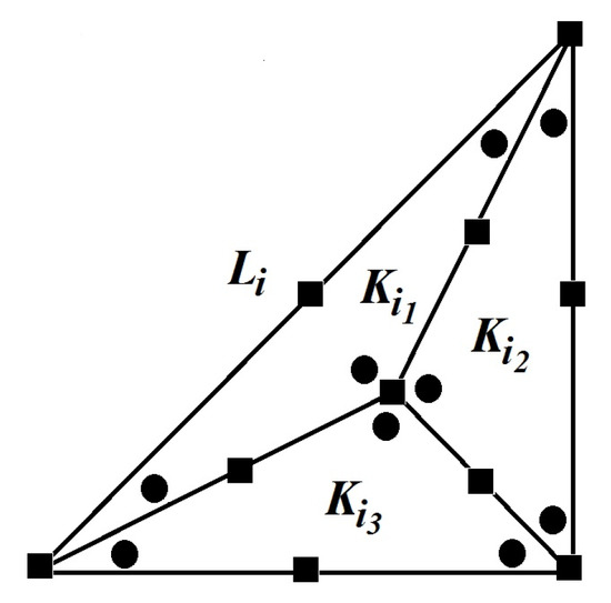
Figure 1. The macro-element $L_i$: squares and dots are the velocity and pressure nodes on $K_{i_j}$, $j=1,2,3,$ respectively.

Now, we define spaces of the SV element pair. The space $X_h,$ for the components of the velocity field, coincides with the corresponding space of degree two of the THelement pair, i.e., $X^h=\{w^h\in C(\Omega ):w^h{|}_{K_{i_j}}\in P_2(K_{i_j}),\forall K_{i_j}\in {{\rm Y}}_h\}$ and for a velocity field ${\mathbf{X}}^h=X^h\times X^h.$ The space $Y^h$, for the pressure, differs from the corresponding space degree one of the TH element pair by the fact that it is discontinuous in $\Omega ,$ i.e., $Y^h=\{y^h\in L_2(\Omega ):y^h{|}_{K_{i_j}}\in P_1(K_{i_j}),\forall K_{i_j}\in {{\rm Y}}_h,\underset{\Omega }{\int }{y}^{h}d\mathbf{x}=0\}.$

The SV element pair has an important property, namely $\mathrm{div}{\mathbf{X}}^h\subset Y^h.$ This means that there exists a function $y^h\in Y^h$ equal to $\mathrm{div}{\mathbf{w}}^h$ such that: from the condition for performing mass conservation in a weak sense, i.e., $\underset{\Omega }{\int }\mathrm{div}{\mathbf{w}}^h{\psi }^{h}d\mathbf{x}=0\forall {\psi }^h\in Y^h$, we get a pointwise mass conservation, i.e., $\parallel \mathrm{div}{\mathbf{w}}^h{\parallel }_{L_2(\Omega )}=0.$ Moreover, in [18], it was established that spaces of the SV element pair before us satisfy the Ladyzhenskaya–Babuška–Brezzi condition. Note, that approximations obtained using the TH element, pair unlike the SV element pair, in general, do not achieve pointwise mass conservation.

Then, we define the weighted basis functions and describe a special finite element method for the Oseen system in the rotation form (8) and (9). For components of the velocity field, for each node $M_k\in G_{\Omega },$ we will match a function:

$${\Phi }_k\left(\mathbf{x}\right)={\rho }^{{\nu }^{\diamond }}\left(\mathbf{x}\right)·{\phi }_k\left(\mathbf{x}\right),k=0,1,\dots ,$$

where ${\phi }_k\left(\mathbf{x}\right)\in X^h,{\phi }_k\left(M_j\right)=\left\{\begin{array}{c}1,k=j,\hfill \\ 0,k\ne j,\hfill \end{array}\right.\hspace{1em}k,j=0,1,\dots$; ${\nu }^{\diamond }$ is a parameter.

We define a set $V^h,$ for components of the velocity field, such that for any velocity field ${\mathbf{v}}^h=(v_1^h,v_2^h),v_i^h\in V^h$, we have:

$$\begin{array}{c}{v}_1^h\left(\mathbf{x}\right)=\sum _k{d}_{2k}{\Phi }_k\left(\mathbf{x}\right),v_2^h\left(\mathbf{x}\right)=\sum _k{d}_{2k+1}{\Phi }_k\left(\mathbf{x}\right),\end{array}$$

(13)

where $d_l={\rho }^{-{\nu }^{\diamond }}\left(M_{[l/2]}\right){\tilde{d}}_l.$

Let $V_0^h$ be a subset in $V^h$ such that $V_0^h=\{w^h\in V^h:w^h\left(M_k\right){|}_{M_k\in G_{\Gamma }}=0\}.$ Moreover, we define velocity field sets ${\mathbf{V}}^h=V^h\times V^h$ and ${\mathbf{V}}_0^h=V_0^h\times V_0^h.$

For the pressure, for each node $N_l\in H,$ we will match a function:

$${\Theta }_m\left(\mathbf{x}\right)={\rho }^{{\mu }^{\diamond }}\left(\mathbf{x}\right)·{\theta }_m\left(\mathbf{x}\right),m=0,1,\dots ,$$

where ${\theta }_m\left(\mathbf{x}\right)\in Y^h,{\theta }_m\left(N_j\right)=\left\{\begin{array}{c}1,m=j,\hfill \\ 0,m\ne j,\hfill \end{array}\right.\hspace{1em}m,j=0,1,\dots ;$ ${\mu }^{\diamond }$ is a parameter.

Then, we define a set $Q^h,$ for the pressure, such that for any $q^h\in Q^h$, we have:

$$\begin{array}{c}{q}^h\left(\mathbf{x}\right)=\sum _m{e}_m{\Theta }_m\left(\mathbf{x}\right),\end{array}$$

(14)

where $e_m={\rho }^{-{\mu }^{\diamond }}\left(N_m\right){\tilde{e}}_m.$

Remark 1.

The coefficients $d_j$ and $e_i$ in (13) and (14) are defined as a solution of a system (17) (see below).

Remark 2.

The following embedding of sets is valid:

$${\mathbf{V}}^h\subset {\mathbf{W}}_{2,\nu }^1({\Omega }_h,\delta ),{\mathbf{V}}_0^h\subset \stackrel{o}{{\mathbf{W}}_{2,\nu }^1}({\Omega }_h,\delta ),Q^h\subset L_{2,\nu }^0({\Omega }_h,\delta ).$$

Definition 2.

The pair $({\mathbf{u}}_{\nu }^h\left(\mathbf{x}\right),P_{\nu }^h\left(\mathbf{x}\right))\in {\mathbf{V}}^h\times Q^h$ is called an approximate $R_{\nu }$-generalized solution for an Oseen system in the rotation form (8) and (9) obtained by the weighted FEM if the equalities:

$$\begin{array}{c}a({\mathbf{u}}_{\nu }^h,{\mathbf{v}}^h)+b({\mathbf{v}}^h,P_{\nu }^h)=l\left({\mathbf{v}}^h\right),\end{array}$$

(15)

$$\begin{array}{c}c({\mathbf{u}}_{\nu }^h,q^h)=0\end{array}$$

(16)

hold for any pair $({\mathbf{v}}^h\left(\mathbf{x}\right),q^h\left(\mathbf{x}\right))\in {\mathbf{V}}_0^h\times Q^h,$ where ${\mathbf{u}}_{\nu }^h=(u_{\nu ,1}^h,u_{\nu ,2}^h)$ and $\omega \in L_{2,\gamma }(\Omega ,\delta ),\mathbf{f}\in {\mathbf{L}}_{2,\gamma }(\Omega ,\delta ),\mathbf{g}\in {\mathbf{W}}_{2,\gamma }^{1/2}(\Gamma ,\delta ),\nu \ge \gamma .$

Thus, we construct a weighted FEM to find an $R_{\nu }$-generalized solution for the rotation form of the Oseen problem (8) and (9).

Then, using (15) and (16), we get a system of linear algebraic equations:

$$\begin{array}{c}\mathbf{A}\mathbf{d}+\mathbf{B}\mathbf{e}=\omega ,{\mathbf{C}}^T\mathbf{d}=\mathbf{z},\end{array}$$

(17)

where $\mathbf{d}={(d_0,d_2,d_4,\dots ,d_1,d_3,d_5,\dots )}^T,\mathbf{e}={(e_0,e_1,e_2,\dots )}^T,\omega ={\mathbf{F}}^h,\mathbf{z}=\mathbf{0}.$

4. Iterative Algorithm

Now, we present an iterative procedure for solving the system of equations (17). Note that the system (17), which needs to be solved, has a large dimension, and moreover, its matrix is sparse. Finding the solution of the system by the direct method is not possible, so that we will construct a convergent iterative process of the following type [19]:

(1)

Let $({\mathbf{d}}^0,{\mathbf{e}}^0)$ be an initial guess for the system (17). We iterate $(n=0,1,2,\dots )$ until the stopping condition is fulfilled;

(2)

Compute ${\mathbf{d}}^{n+1}={\mathbf{d}}^n+{\widehat{\mathbf{A}}}^{-1}(\omega -\mathbf{A}{\mathbf{d}}^n-\mathbf{B}{\mathbf{e}}^n)$;

(3)

Find ${\mathbf{e}}^{n+1}={\mathbf{e}}^n+{\widehat{\mathbf{S}}}^{-1}({\mathbf{C}}^T{\mathbf{d}}^{n+1}-\mathbf{z})$;

where $\widehat{\mathbf{A}}$ is a preconditioning matrix to $\mathbf{A}$ and $\widehat{\mathbf{S}}$ is a preconditioning matrix to $\mathbf{S}={\mathbf{C}}^T{\mathbf{A}}^{-1}\mathbf{B}$, which is called the Schur complement matrix. Next, we describe the process of constructing preconditioning matrices $\widehat{\mathbf{A}}$ and $\widehat{\mathbf{S}}.$

At first, we build a preconditioner $\widehat{\mathbf{A}}$ applying an incomplete $\mathbf{LU}$ factorization, where $\mathbf{L}$ and $\mathbf{U}$ are low unitriangular and upper triangular matrices respectively. At each iteration in Item 2, we employ the GMRES(l) method (see [20]) as the solution of a problem $\mathbf{A}\mathbf{v}=\mathbf{s}$ with the left preconditioner $\widehat{\mathbf{A}}$. The method is designed so that it approximates the solution in an $l^{\mathrm{th}}$ order Krylov subspace. In our research, the dimension of a Krylov subspace is equal to 10; so that if ${\mathbf{r}}_0={\widehat{\mathbf{A}}}^{-1}(\mathbf{s}-\mathbf{A}\mathbf{v})$, then the Arnoldi procedure will build an orthonormal basis of the subspace: $\mathrm{Span}\{{\mathbf{r}}_0,{({\widehat{\mathbf{A}}}^{-1}\mathbf{A})}^1{\mathbf{r}}_0,\dots ,({\widehat{\mathbf{A}}}^{-1}\mathbf{A}{)}^9{\mathbf{r}}_0\}$.

Secondly, we build an intermediate matrix $\tilde{\mathbf{S}}$ to $\widehat{\mathbf{S}}.$ The matrix $\tilde{\mathbf{S}}$ represents a mass matrix ${\mathbf{M}}_P^{\overline{\nu },{\mu }^{\diamond },\nu }$ of a special view, such that on all elements $K\in {{\rm Y}}_h:$

$${({\mathbf{M}}_P^{\overline{\nu },{\mu }^{\diamond },\nu })}_{ij}=\frac{1}{\overline{\nu }}\underset{K}{\int }{\rho }^{2(\nu +{\mu }^{\diamond })}{\theta }_j\left(\mathbf{x}\right){\theta }_i\left(\mathbf{x}\right)d\mathbf{x},{\theta }_j\left(\mathbf{x}\right),{\theta }_i\left(\mathbf{x}\right)\in Y^h,j,i=0,1,\dots .$$

After that, we determine a matrix $\overline{\mathbf{S}}$, which is equal to a diagonal matrix ${\overline{\mathbf{M}}}_P^{\overline{\nu },{\mu }^{\diamond },\nu }$ with elements ${({\overline{\mathbf{M}}}_P^{\overline{\nu },{\mu }^{\diamond },\nu })}_{ii}={\displaystyle \sum _k}{({\mathbf{M}}_P^{\overline{\nu },{\mu }^{\diamond },\nu })}_{ik}$. In other words, ${\left(\overline{\mathbf{S}}\right)}_{ii}={\displaystyle \sum _k}{(\tilde{\mathbf{S}})}_{ik}$. It is known (see [9] and the references therein) that such diagonal lumping $\overline{\mathbf{S}}$ is a good preconditioner to the initial matrix $\tilde{\mathbf{S}}$.

Therefore, in order to determine the vector ${\Psi }^{🟉}:={\widehat{\mathbf{S}}}^{-1}\chi ,$ at each iteration of Item 3, we must find a solution to the following internal procedure: (1) ${\varphi }^0=\mathbf{0}$; (2) ${\varphi }^m={\varphi }^{m-1}+{\overline{\mathbf{S}}}^{-1}(\chi -\tilde{\mathbf{S}}{\varphi }^{m-1})(m=1,\dots ,M)$; (3) ${\Psi }^{🟉}={\varphi }^M.$

We apply the GMRES(5) method, where $\mathrm{Span}\{\overline{\mathbf{r}},{({\overline{\mathbf{S}}}^{-1}\tilde{\mathbf{S}})}^1\overline{\mathbf{r}},\dots ,{({\overline{\mathbf{S}}}^{-1}\tilde{\mathbf{S}})}^4\overline{\mathbf{r}}\}$, and $\overline{\mathbf{r}}={\overline{\mathbf{S}}}^{-1}(\chi -\tilde{\mathbf{S}}{\varphi }^{m-1})$.

5. Numerical Experiments

Now, we present numerical results for the Oseen system in the rotation form (8) and (9) and show the advantage of the proposed method.

Let ${\Omega }_k=(-l;l)\times (-l;l)\backslash {\overline{G}}_k$ be a polygon with one internal corner greater than ${180}^{\circ }$ on ${\Gamma }_k$ whose vertex is at the origin. We will consider the following sizes of the reentrant corner: ${\omega }_k=\frac{2^k+1}{2^k}\pi ,k=1,2,3.$ The triangulation ${{\rm Y}}_h$ (see Section 3) of each ${\overline{\Omega }}_k,k=1,2,3$ and $l=1$ we present in Figure 2.

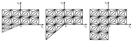
Figure 2. The triangulation ${{\rm Y}}_h$ of a domain ${\overline{\Omega }}_k$.

In a test problem, we consider the solution of the problem (8), (9), which has a singularity in a neighborhood of a point located at the origin. Let $\alpha =\overline{\nu }=1,w=b·\mathrm{curl}\mathbf{u},b=0.95$, and for each corner ${\omega }_k$ in polar coordinates $(r,\phi )$, we have an auxiliary function:

$${\Psi }_k\left(\phi \right)=\frac{\sin \left((1+{\lambda }_k)\phi \right)\cos \left({\lambda }_k{\omega }_k\right)}{1+{\lambda }_k}-\frac{\sin \left((1-{\lambda }_k)\phi \right)\cos \left({\lambda }_k{\omega }_k\right)}{1-{\lambda }_k}+\cos \left((1-{\lambda }_k)\phi \right)-\cos \left((1+{\lambda }_k)\phi \right).$$

Then, the exact solution $\mathbf{u}=(u_1,u_2)$ and P of the problem (8) and (9) for each corner ${\omega }_k,k=1,2,3,$ in polar coordinates has the following form:

$$u_1(r,\phi )=r^{{\lambda }_k}·(({\lambda }_k+1)\sin \phi ·{\Psi }_k\left(\phi \right)+\cos \phi ·{\Psi }_k^{\prime }\left(\phi \right)),$$

$$u_2(r,\phi )=r^{{\lambda }_k}·(\sin \phi ·{\Psi }_k^{\prime }\left(\phi \right)-({\lambda }_k+1)\cos \phi ·{\Psi }_k\left(\phi \right)),$$

$$P(r,\phi )=r^{{\lambda }_k-1}·\frac{{({\lambda }_k+1)}^2{\Psi }_k^{\prime }\left(\phi \right)+{\Psi }_k^{‴}\left(\phi \right)}{{\lambda }_k-1},$$

where ${\lambda }_k=min\{\lambda :\sin \left(\lambda {\omega }_k\right)+\lambda \sin {\omega }_k=0\mathrm{and}\lambda >0\}$.

Thus, for the corner ${\omega }_1=\frac{3\pi }{2}$, we have ${\lambda }_1\approx 0.544483,$ for ${\omega }_2=\frac{5\pi }{4}$, ${\lambda }_2\approx 0.673583$, and for ${\omega }_3=\frac{9\pi }{8}$, ${\lambda }_3\approx 0.800766.$ The proposed solution is analytical in ${\overline{\Omega }}_k\backslash (0,0),$ but unfortunately, $P\notin W_2^1\left({\Omega }_k\right),\mathbf{u}\notin {\mathbf{W}}_2^2\left({\Omega }_k\right).$

In numerical experiments, we use meshes with a various step size h and number N, where $N·h$ equals two. The approximate generalized solution (velocity field) by classical FEM converges to the exact one in the ${\mathbf{W}}_2^1\left({\Omega }_k\right)$ norm with a rate depending on the size of reentrant corner $\omega$, the so-called pollution effect (see [12] and the references therein): for a corner ${\omega }_1=\frac{3\pi }{2}$, we have the rate of convergence, which is equal to $\mathcal{O}(h^{0.55})$, for a corner ${\omega }_2=\frac{5\pi }{4}$, $\mathcal{O}(h^{0.67})$, and for a corner ${\omega }_3=\frac{9\pi }{8}$, $\mathcal{O}(h^{0.8})$ (see Table 1); whereas, the approximate $R_{\nu }$-generalized solution by the presented weighted FEM converges to the exact one in the ${\mathbf{W}}_{2,\nu }^1\left({\Omega }_k\right)$ norm with a rate that is independent of the value of the internal angle $\omega$ and has the first order by h (see Table 2), where we derive computationally the optimal parameters $\delta ,{\nu }^{\diamond }={\nu }_{opt}^{\diamond }$ and $\nu$. Both errors for the $R_{\nu }$-generalized and generalized solutions visually are represented in Figure 3 for different values of a number N.

Table 1. The generalized solution error $({\mathbf{u}}^h-\mathbf{u})$ in the norm of a space ${\mathbf{W}}_2^1\left({\Omega }_k\right).$

${\mathbf{\omega }}_{\mathit{k}}$, $\mathit{N}=$	74	148	296
$\frac{3\pi }{2}$	2.886 $\times {10}^{-1}$	1.980 $\times {10}^{-1}$	1.358 $\times {10}^{-1}$
$\frac{5\pi }{4}$	1.622 $\times {10}^{-1}$	1.017 $\times {10}^{-1}$	6.377 $\times {10}^{-2}$
$\frac{9\pi }{8}$	6.747 $\times {10}^{-2}$	3.870 $\times {10}^{-2}$	2.220 $\times {10}^{-2}$

Table 2. The $R_{\nu }$-generalized solution error $({\mathbf{u}}_{\nu }^h-{\mathbf{u}}_{\nu })$ in the norm of a space ${\mathbf{W}}_{2,\nu }^1\left({\Omega }_k\right),$ where ${\nu }^{\diamond }={\mu }^{\diamond }={\lambda }_k-1$ and ${\nu }^{\diamond }={\mu }^{\diamond }={\nu }_{opt}^{\diamond }.$

			${\mathbf{\nu }}^{\diamond }={\mathbf{\mu }}^{\diamond }={\mathbf{\lambda }}_{\mathit{k}}-1$			${\mathbf{\nu }}^{\diamond }={\mathbf{\mu }}^{\diamond }={\mathbf{\nu }}_{\mathit{opt}}^{\diamond }$
${\mathbf{\omega }}_{\mathit{k}}$	$\mathbf{\nu }$	$\mathbf{\delta }$, $\mathit{N}=$	74	148	296	74	148	296
$\frac{3\pi }{2}$	1.6	0.01375	2.261 $\times {10}^{-4}$	1.126 $\times {10}^{-4}$	5.504 $\times {10}^{-5}$	1.614 $\times {10}^{-5}$	8.026 $\times {10}^{-5}$	3.991 $\times {10}^{-5}$
		0.01625	3.181 $\times {10}^{-4}$	1.582 $\times {10}^{-4}$	7.895 $\times {10}^{-5}$	2.290 $\times {10}^{-4}$	1.138 $\times {10}^{-4}$	5.648 $\times {10}^{-5}$
	1.9	0.01375	6.236 $\times {10}^{-5}$	3.101 $\times {10}^{-5}$	1.543 $\times {10}^{-5}$	4.469 $\times {10}^{-5}$	2.235 $\times {10}^{-5}$	1.109 $\times {10}^{-5}$
		0.01625	9.311 $\times {10}^{-5}$	4.601 $\times {10}^{-5}$	2.288 $\times {10}^{-5}$	6.789 $\times {10}^{-5}$	3.381 $\times {10}^{-5}$	1.675 $\times {10}^{-5}$
$\frac{5\pi }{4}$	1.6	0.01375	1.181 $\times {10}^{-4}$	5.849 $\times {10}^{-5}$	2.925 $\times {10}^{-5}$	9.247 $\times {10}^{-5}$	4.603 $\times {10}^{-5}$	2.276 $\times {10}^{-5}$
		0.01625	1.720 $\times {10}^{-4}$	8.568 $\times {10}^{-5}$	4.275 $\times {10}^{-5}$	1.322 $\times {10}^{-4}$	6.567 $\times {10}^{-5}$	3.260 $\times {10}^{-5}$
	1.9	0.01375	3.320 $\times {10}^{-5}$	1.651 $\times {10}^{-5}$	8.234 $\times {10}^{-6}$	2.605 $\times {10}^{-5}$	1.293 $\times {10}^{-5}$	6.437 $\times {10}^{-6}$
		0.01625	5.115 $\times {10}^{-5}$	2.547 $\times {10}^{-5}$	1.262 $\times {10}^{-5}$	3.835 $\times {10}^{-5}$	1.905 $\times {10}^{-5}$	9.513 $\times {10}^{-6}$
$\frac{9\pi }{8}$	1.6	0.01375	6.020 $\times {10}^{-5}$	2.993 $\times {10}^{-5}$	1.495 $\times {10}^{-5}$	4.493 $\times {10}^{-5}$	2.233 $\times {10}^{-5}$	1.104 $\times {10}^{-5}$
		0.01625	7.947 $\times {10}^{-5}$	3.946 $\times {10}^{-5}$	1.959 $\times {10}^{-5}$	6.124 $\times {10}^{-5}$	3.036 $\times {10}^{-5}$	1.497 $\times {10}^{-5}$
	1.9	0.01375	1.684 $\times {10}^{-5}$	8.366 $\times {10}^{-6}$	4.170 $\times {10}^{-6}$	1.239 $\times {10}^{-5}$	6.158 $\times {10}^{-6}$	3.068 $\times {10}^{-6}$
		0.01625	2.364 $\times {10}^{-5}$	1.174 $\times {10}^{-5}$	5.800 $\times {10}^{-6}$	1.756 $\times {10}^{-5}$	8.708 $\times {10}^{-6}$	4.324 $\times {10}^{-6}$

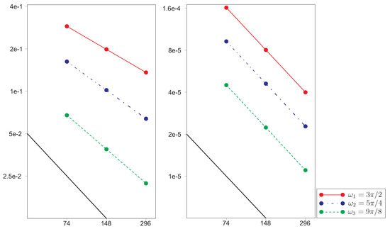
Figure 3. The errors of (left) a classical FEM in the ${\mathbf{W}}_2^1$ norm and (right) a weighted FEM in the ${\mathbf{W}}_{2,\nu }^1$ norm, where $\nu =1.6,\delta =0.01375:{\omega }_1=\frac{3\pi }{2},{\nu }^{\diamond }={\nu }_{opt}=-0.35;{\omega }_2=\frac{5\pi }{4},{\nu }^{\diamond }={\nu }_{opt}=-0.25$; ${\omega }_3=\frac{9\pi }{8},{\nu }^{\diamond }={\nu }_{opt}=-0.125$, for different values of a number N.

Let ${\delta }_{ji}^{\prime }=|u_j\left(M_i\right)-u_j^h\left(M_i\right)|$ and ${\delta }_{ji}=|u_j\left(M_i\right)-u_{\nu ,j}^h\left(M_i\right)|,j=1,2,M_i\in G_{\Omega }$ be errors for the generalized and $R_{\nu }$-generalized solutions, respectively. Then, we show the percentage of nodes, where ${\delta }_{1i}^{\prime }$ and ${\delta }_{1i}$ are less than a given value ${\overline{\Delta }}_l$. The quantity of points $M_i\in G_{\Omega }$, where ${\delta }_{1j}^{\prime }<{\overline{\Delta }}_l$ (for the classical FEM), is significantly less in relation to the quantity of points $M_i\in G_{\Omega }$, where ${\delta }_{1j}<{\overline{\Delta }}_l$ (for the proposed weighted FEM) for all sizes of the reentrant corner $\omega$ (see Table 3). Moreover, in numerical experiments, the number of nodes $M_i,$ where ${\delta }_{2i}^{\prime }<{\overline{\Delta }}_l$ and ${\delta }_{2i}<{\overline{\Delta }}_l$ are approximately equal to the number of nodes $M_i,$ where ${\delta }_{1i}^{\prime }<{\overline{\Delta }}_l$ and ${\delta }_{1i}<{\overline{\Delta }}_l$, $l=1,2,$ respectively.

Table 3. The percentage of points $M_i\in G_{\Omega },$ where the values ${\delta }_{1i}$ and ${\delta }_{1i}^{\prime }$ are less than ${\overline{\Delta }}_l,l=1,2.$

		${\mathbf{R}}_{\mathbf{\nu }}$-Generalized Solution, $\mathbf{\nu }=1.9,$ $\mathbf{\delta }=\mathbf{0.01375},{\mathbf{\nu }}^{\diamond }={\mathbf{\mu }}^{\diamond }={\mathbf{\nu }}_{\mathit{opt}}^{\diamond }$			Generalized Solution
${\omega }_k$	${\overline{\Delta }}_l,N=$	74	148	296	74	148	296
$\frac{3\pi }{2}$	${10}^{-5}$	19.1%	36.7%	65.7%	13.2%	14.8%	22.1%
	$5\times {10}^{-6}$	16.4%	29.3%	51.4%	6.2%	9.1%	15.6%
$\frac{5\pi }{4}$	${10}^{-5}$	33.9%	51.0%	76.2%	21.4%	32.4%	44.2%
	$5\times {10}^{-6}$	24.1%	42.4%	64.7%	11.4%	17.5%	27.4%
$\frac{9\pi }{8}$	${10}^{-5}$	60.3%	91.5%	98.1%	44.7%	68.3%	86.4%
	$5\times {10}^{-6}$	39.7%	62.7%	80.5%	24.8%	32.7%	44.3%

Then, we present the distribution of errors ${\delta }_{ji}$ and ${\delta }_{ji}^{\prime }$ in the points $M_k$ for components $u_{\nu ,j}^h$ and $u_j^h$ for all sizes ${\omega }_l,l=1,2,3,j=1,2$, and $h,$ such that $N=148$ and $N=296$. The weighted finite element method allows us to perform computations with high accuracy both inside of the domain and near the point of singularity. Moreover, the error of the proposed FEM is localized near the point of singularity and does not extend into the interior of the domain, in contrast to the error of the classical FEM for all values of the internal corner $\omega$ (see Figure 4, Figure 5, Figure 6, Figure 7, Figure 8, Figure 9, Figure 10, Figure 11, Figure 12, Figure 13, Figure 14 and Figure 15).

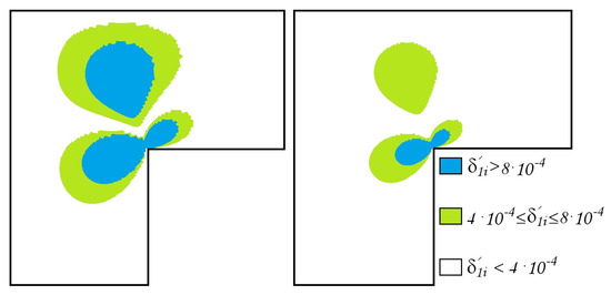
Figure 4. The errors ${\delta }_{1i}^{\prime }$ of the approximate generalized solution $(u_1^h):{\omega }_1=\frac{3\pi }{2}$, (left) $N=148$, (right) $N=296$.

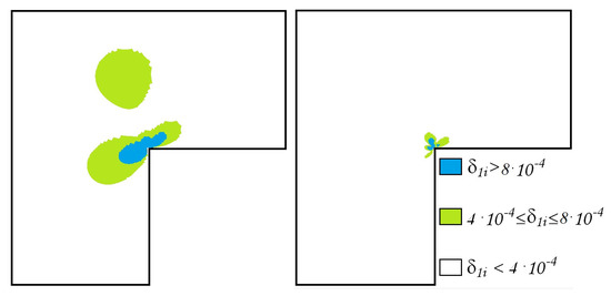
Figure 5. The errors ${\delta }_{1i}$ of the approximate $R_{\nu }$-generalized solution $(u_{\nu ,1}^h):{\omega }_1=\frac{3\pi }{2},\nu =1.6$, $\delta =0.01375,{\nu }^{\diamond }={\mu }^{\diamond }=-0.35$, (left) $N=148$, (right) $N=296$.

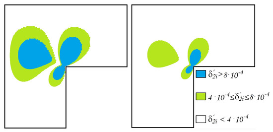
Figure 6. The distribution of the errors ${\delta }_{2i}^{\prime }$ of the approximate generalized solution $(u_2^h):{\omega }_1=\frac{3\pi }{2}$, (left) $N=148$, (right) $N=296$.

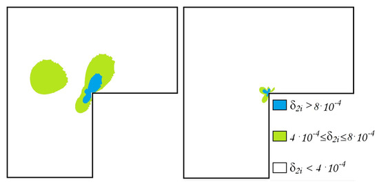
Figure 7. The errors ${\delta }_{2i}$ of the approximate $R_{\nu }$-generalized solution $(u_{\nu ,2}^h):{\omega }_1=\frac{3\pi }{2},\nu =1.6$, $\delta =0.01375,{\nu }^{\diamond }={\mu }^{\diamond }=-0.35$, (left) $N=148$, (right) $N=296$.

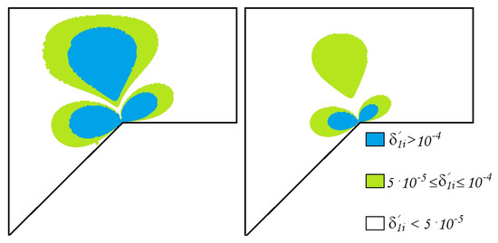
Figure 8. The errors ${\delta }_{1i}^{\prime }$ of the approximate generalized solution $(u_1^h):{\omega }_2=\frac{5\pi }{4}$, (left) $N=148$, (right) $N=296$.

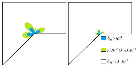
Figure 9. The errors ${\delta }_{1i}$ of the approximate $R_{\nu }$-generalized solution $(u_{\nu ,1}^h):{\omega }_2=\frac{5\pi }{4},\nu =1.6$, $\delta =0.01375,{\nu }^{\diamond }={\mu }^{\diamond }=-0.25$, (left) $N=148$, (right) $N=296$.

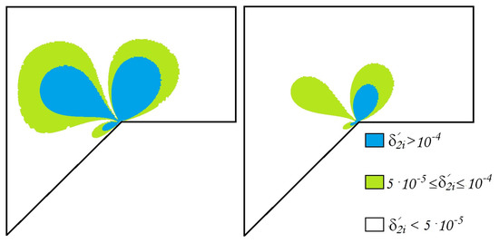
Figure 10. The errors ${\delta }_{2i}^{\prime }$ of the approximate generalized solution $(u_2^h):{\omega }_2=\frac{5\pi }{4},$ (left) $N=148$, (right) $N=296$.

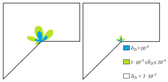
Figure 11. The errors ${\delta }_{2i}$ of the approximate $R_{\nu }$-generalized solution $(u_{\nu ,2}^h):{\omega }_2=\frac{5\pi }{4},\nu =1.6$, $\delta =0.01375,{\nu }^{\diamond }={\mu }^{\diamond }=-0.25$, (left) $N=148$, (right) $N=296$.

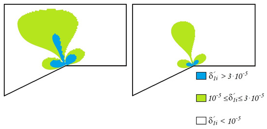
Figure 12. The errors ${\delta }_{1i}^{\prime }$ of the approximate generalized solution $(u_1^h):{\omega }_3=\frac{9\pi }{8},$ (left) $N=148$, (right) $N=296$.

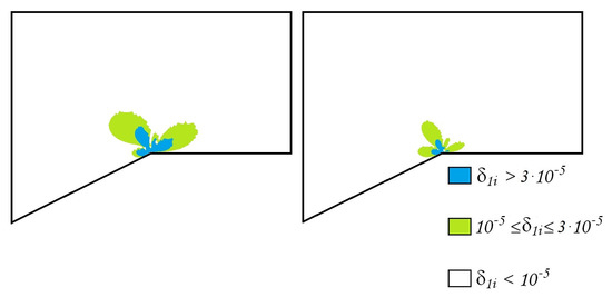
Figure 13. The errors ${\delta }_{1i}$ of the approximate $R_{\nu }$-generalized solution $(u_{\nu ,1}^h):{\omega }_3=\frac{9\pi }{8},\nu =1.6$, $\delta =0.01375,{\nu }^{\diamond }={\mu }^{\diamond }=-0.125$, (left) $N=148$, (right) $N=296$.

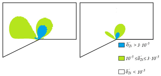
Figure 14. The errors ${\delta }_{2i}^{\prime }$ of the approximate generalized solution $(u_2^h):{\omega }_3=\frac{9\pi }{8}$, (left) $N=148$, (right) $N=296$.

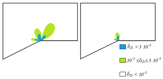
Figure 15. The errors ${\delta }_{2i}$ of the approximate $R_{\nu }$-generalized solution $(u_{\nu ,2}^h):{\omega }_3=\frac{9\pi }{8},\nu =1.6$, $\delta =0.01375,{\nu }^{\diamond }={\mu }^{\diamond }=-0.125$, (left) $N=148$, (right) $N=296$.

In Figure 16, Figure 17 and Figure 18, we show the dependence of error in the ${\mathbf{W}}_{2,\nu }^1\left({\Omega }_k\right)$ norm on the parameter ${\nu }^{\diamond }$ (${\mu }^{\diamond }={\nu }^{\diamond }$), where each minimum is compatible with the best value ${\nu }_{opt}^{\diamond }$. Any value from the interval $({\lambda }_k-1,0)$ can be taken as an exponent ${\nu }^{\diamond }$ for the presented FEM in the domain ${\Omega }_k$ with a reentrant corner ${\omega }_k$. Moreover, if the exponent ${\mu }^{\diamond }$ does not coincide with ${\nu }^{\diamond },$ then we get substantially worse results. This research was supported in through computational research provided by the Shared Facility Center “Data Center of FEB RAS”.

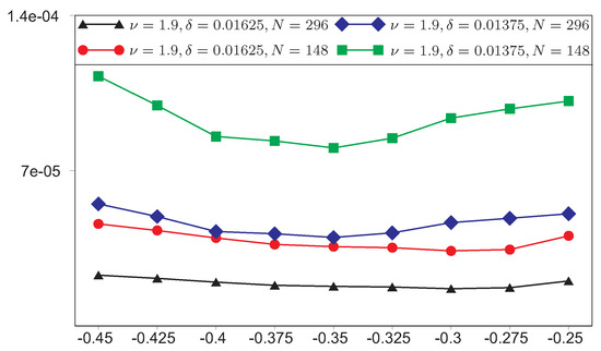
Figure 16. The dependence of error $({\mathbf{u}}_{\nu }^h-\mathbf{u})$ in the ${\mathbf{W}}_{2,\nu }^1\left({\Omega }_1\right)$ norm on the degree ${\nu }^{\diamond }$, ${\omega }_1=\frac{3\pi }{2}.$

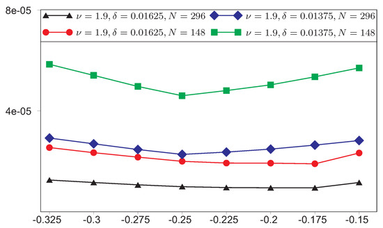
Figure 17. The dependence of error $({\mathbf{u}}_{\nu }^h-\mathbf{u})$ in the ${\mathbf{W}}_{2,\nu }^1\left({\Omega }_2\right)$ norm on the degree ${\nu }^{\diamond }$, ${\omega }_2=\frac{5\pi }{4}.$

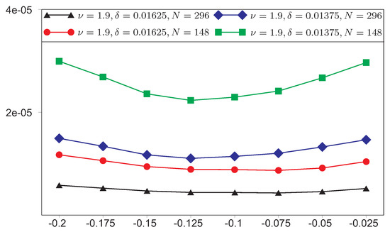
Figure 18. The dependence of error $({\mathbf{u}}_{\nu }^h-\mathbf{u})$ in the ${\mathbf{W}}_{2,\nu }^1\left({\Omega }_3\right)$ norm on the degree ${\nu }^{\diamond }$, ${\omega }_3=\frac{9\pi }{8}.$

6. Conclusions

The main results of the numerical experiments for the Oseen problem (8) and (9) lead to the following conclusions:

• The approximate generalized solution (velocity field) by classical FEM converges to the exact one in the ${\mathbf{W}}_2^1\left({\Omega }_k\right)$ norm with a rate $\mathcal{O}(h^{\lambda }),\lambda <1,$ where the exponent $\lambda$ depends on the size of reentrant corner $\omega$, the so-called pollution effect (see [12] and the references therein), while the approximate $R_{\nu }$-generalized solution by the presented weighted FEM converges to the exact one in the ${\mathbf{W}}_{2,\nu }^1$ norm with a rate that is independent of the value of the internal angle $\omega$ and has the first order by h for various values of $\nu ,\delta$ (see Table 1 and Table 2 and Figure 3).
• Thanks to Theorem 3.1 in [13], there exists a limitation on the radius ${\delta }_{*}$ of the neighborhood of a reentrant corner $\omega$ and $\rho \left(\mathbf{x}\right)$ exponent ${\nu }_{*}$ in Definition 1, that for all $\delta <{\delta }_{*}$ and $\nu >{\nu }_{*}$, a weighted $\mathrm{inf-sup}$ condition holds. After a series of computational experiments, we conclude that ${\nu }_{*}\sim 1$ and ${\delta }_{*}\sim h$.
• The proposed approach allows us to compute the approximate solution by the weighted FEM with a given accuracy ${10}^{-3}$, for example in a case when the internal corner $\omega$ is equal to $\frac{3\pi }{2}$, about ${10}^6$-times faster than using classical FEM. Note that in implementing the weighted FEM, one can spend about ${10}^6$-times less computing resources and energy consumption.
• The weighted finite element method enables us to perform computations with high accuracy, both inside of the domain and near the point of singularity.

References

- Ciarlet, P. The Finite Element Method for Elliptic Problems; Studies in Mathematics and Its Applications; North-Holland: Amsterdam, The Netherlands, 1978. [Google Scholar]
- Rukavishnikov, V.A. On the differential properties of Rν-generalized solution of Dirichlet problem. Dokl. Akad. Nauk SSSR 1989, 309, 1318–1320. [Google Scholar]
- Rukavishnikov, V.A.; Rukavishnikova, H.I. The finite element method for a boundary value problem with strong singularity. J. Comput. Appl. Math. 2010, 234, 2870–2882. [Google Scholar] [CrossRef]
- Rukavishnikov, V.A.; Mosolapov, A.O. New numerical method for solving time-harmonic Maxwell equations with strong singularity. J. Comput. Phys. 2012, 231, 2438–2448. [Google Scholar] [CrossRef]
- Rukavishnikov, V.A.; Rukavishnikova, H.I. On the error estimation of the finite element method for the boundary value problems with singularity in the Lebesgue weighted space. Numer. Funct. Anal. Optim. 2013, 34, 1328–1347. [Google Scholar] [CrossRef]
- Rukavishnikov, V.A. Weighted FEM for Two-Dimensional Elasticity Problem with Corner Singularity; Lecture Notes in Computational Science and Engineering; Oxford University Press: Oxford, UK, 2016; Volume 112, pp. 411–419. [Google Scholar] [CrossRef]
- Rukavishnikov, V.A.; Rukavishnikova, H.I. Weighted Finite-Element Method for Elasticity Problems with Singularity; Finite Element Method Simulation, Numerical Analysis and Solution Techniques; IntechOpen Limited: London, UK, 2018; pp. 295–311. [Google Scholar] [CrossRef]
- Benzi, M.; Golub, G.H.; Liesen, J. Numerical solution of saddle point problems. Acta Numer. 2005, 14, 1–137. [Google Scholar] [CrossRef]
- Layton, W.; Manica, C.; Neda, M.; Olshanskii, M.; Rebholz, L.G. On the accuracy of the rotation form in simulations of the Navier-Stokes equations. J. Computat. Phys. 2009, 228, 3433–3447. [Google Scholar] [CrossRef]
- Moffatt, H.K. Viscous and resistive eddies near a sharp corner. J. Fluid Mech. 1964, 18, 1–18. [Google Scholar] [CrossRef]
- Dauge, M. Stationary Stokes and Navier-Stokes system on two- or three-dimensional domains with corners. I. Linearized equations. SIAM J. Math. Anal. 1989, 20, 74–97. [Google Scholar] [CrossRef]
- Blum, H. The influence of reentrant corners in the numerical approximation of viscous flow problems. In Numerical Treatment of the Navier-Stokes Equations; Springer: Berlin, Germany, 1990; Volume 30. [Google Scholar] [CrossRef]
- Rukavishnikov, V.A.; Rukavishnikov, A.V. Weighted finite element method for the Stokes problem with corner singularity. J. Comput. Appl. Math. 2018, 341, 144–156. [Google Scholar] [CrossRef]
- Brezzi, F.; Fortin, M. Mixed and Hybrid Finite Element Methods; Springer-Verlag: New York, NY, USA, 1991. [Google Scholar] [CrossRef]
- Rukavishnikov, V.A.; Rukavishnikov, A.V. New approximate method for solving the Stokes problem in a domain with corner singularity. Bull. South Ural State Univ. Ser. Math. Model. Program. Comput. Softw. 2018, 11, 95–108. [Google Scholar] [CrossRef]
- Scott, L.R.; Vogelius, M. Norm estimates for a maximal right inverse of the divergence operator in spaces of piecewise polynomials. Math. Model. Numer. Anal. 1985, 19, 111–143, MR 813691. [Google Scholar]
- Linke, A. Collision in a cross-shaped domain—A steady 2D Navier-Stokes example demonstrating the importance of mass conservation in CFD. Comput. Methods Appl. Mech. Eng. 2009, 198, 3268–3278. [Google Scholar] [CrossRef]
- Qin, J. On the Convergence of Some Low Order Mixed Finite Element for Incompressible Fluids. Ph.D. Thesis, Pennsylvania State University, University Park, PA, USA, 1994. [Google Scholar] [CrossRef]
- Bramble, J.H.; Pasciak, J.E.; Vassilev, A.T. Analysis of the inexact Uzawa algorithm for saddle point problems. SIAM J. Numer. Anal. 1997, 34, 1072–1092. [Google Scholar] [CrossRef]
- Saad, Y. Iterative Methods for Sparse Linear Systems; Society for Industrial and Applied Mathematics: Philadelphia, PA, USA, 2003. [Google Scholar] [CrossRef]
© 2019 by the authors. Licensee MDPI, Basel, Switzerland. This article is an open access article distributed under the terms and conditions of the Creative Commons Attribution (CC BY) license (http://creativecommons.org/licenses/by/4.0/).