Generalized Modified Slash Birnbaum–Saunders Distribution

Abstract

In this paper, a generalization of the modified slash Birnbaum–Saunders (BS) distribution is introduced. The model is defined by using the stochastic representation of the BS distribution, where the standard normal distribution is replaced by a symmetric distribution proposed by Reyes et al. It is proved that this new distribution is able to model more kurtosis than other extensions of BS previously proposed in the literature. Closed expressions are given for the pdf (probability density functio), along with their moments, skewness and kurtosis coefficients. Inference carried out is based on modified moments method and maximum likelihood (ML). To obtain ML estimates, two approaches are considered: Newton–Raphson and EM-algorithm. Applications reveal that it has potential for doing well in real problems.

1. Introduction

The BS distribution was introduced by Birnbaum and Saunders [1,2]. The aim of this distribution is to model the fatigue in lifetime of certain materials. Nowadays, its use has spread to other contexts such as economic and environmental data. In these new applications, it is quite common to find real datasets in which a BS model with heavier tails would be suitable. Slash models are a good option to deal with this kind of situations, in which heavy tails are a serious problem for the data analyst. This is the main reason slash distributions have received a great deal of attention during the last decades. In this context, we face the problem of improving BS distribution by introducing a generalization able to model more kurtosis than other slash extensions previously proposed in the literature. In these extensions, the emphasis is on kurtosis because, as Moors [3] pointed out, the presence of heavy tails produces high kurtosis. Next, we briefly describe the BS-model and the most relevant slash precedents of our proposal.

1.1. Birnbaum–Saunders Distribution

If a random variable (rv) $T>0$ follows a BS distribution with shape parameter $\alpha >0$ and scale parameter $\beta >0$, $T\sim BS(\alpha ,\beta )$, then T can be expressed as

$$\begin{array}{c}\hfill T=\beta {\left(\frac{\alpha }{2}Z+\sqrt{{\left(\frac{\alpha }{2}Z\right)}^2+1}\right)}^2\end{array}$$

(1)

where $Z\sim N(0,1)$. From Equation (1), T is a monotone transformation of Z, and its cumulative distribution function (cdf) $F_T$ is

$$F_T\left(t\right)=\mathsf{\Phi }\left(w\left(t\right)\right)$$

(2)

with $\mathsf{\Phi }(·)$ the cdf of a $N(0,1)$ distribution and

$$w\left(t\right)=w_{\alpha ,\beta }\left(t\right)=\frac{1}{\alpha }\left(\sqrt{\frac{t}{\beta }}-\sqrt{\frac{\beta }{t}}\right)=\frac{2}{\alpha }sinh\left(ln\sqrt{\frac{t}{\beta }}\right),t>0.$$

(3)

The probability density function (pdf) of T is

$$f_T(t;\alpha ,\beta )=\frac{t^{-\frac{3}{2}}(t+\beta )}{2\alpha {\beta }^{\frac{1}{2}}}\varphi \left(w\left(t\right)\right)$$

(4)

where $\varphi (·)$ is the pdf of a $N(0,1)$ distribution (Johnson et al. [4]).

As properties (see, for instance, Leiva [5]), we highlight that the BS distribution is continuous, unimodal and positively skewed (asymmetry to right). $\beta$ is the median of the distribution. $\alpha$ is a shape parameter that modifies the skewness and kurtosis of the distribution. As $\alpha$ tends to zero, the BS distribution tends to be symmetrical around $\beta$ and its variability decreases. On the other hand, as $\alpha$ increases, the BS distribution exhibits heavier tails.

1.2. Slash Methodology

To use the BS distribution for modeling data with outliers, Gómez et al. [6] and Reyes et al. [7] proposed extensions of BS model based on the slash (S) and modified slash (MS) distribution. In this way, they got extensions of BS distribution with a high kurtosis coefficient.

The canonic slash distribution was introduced by Rogers and Tukey [8]. This model is defined as the ratio of a $N(0,1)$ and an independent uniform $U(0,1)$ distribution. It is proposed as a model for bell-shaped data with heavier tails than the corresponding normal distribution. Their theoretical properties can be seen, for instance, in Rogers and Tukey [8] or Johnson et al. [4]. The slash model, denoted as S, in which a kurtosis parameter q is introduced, is defined as

$$\begin{array}{c}\hfill S=\frac{Z}{U^{\frac{1}{q}}}\end{array}$$

(5)

with $Z\sim N(0,1)$ independent of $U\sim U(0,1)$ and $q>0$. Based on the representation given in Equation (5), Reyes et al. [7] proposed the modified slash (MS) distribution in which the variable at the denominator of Equation (5) is replaced by an exponential distribution of parameter 2, that is, $U\sim Exp\left(2\right)$. The MS model exhibits greater kurtosis than the S model. A new extension, called generalized modified slash (GMS) distribution, was introduced recently by Reyes et al. [9]. These authors proposed a new slash model where the denominator in Equation (5) is a Gamma distribution of parameters ($2q,q$) with $q>0$. The GMS model generalizes the MS model. As main features of the GMS model, we highlight that is a bell-shaped distribution, symmetrical with respect to zero, and exhibits a greater level of kurtosis than its predecessors, thus it can be of interest to study the distribution of the BS extension obtained when $Z\sim N(0,1)$ in Equation (1) is replaced by a GMS distribution with kurtosis parameter $q>0$. This proposal is a generalization of the papers by Gómez et al. [6] and Reyes et al. [7] where slash versions of the BS distribution were considered based on the slash and modified slash distribution, called slash Birnbaum–Saunders (SBS) and modified slash Birnbaum–Saunders (MSBS), respectively.

This paper is outlined as follows. In Section 2, the stochastic representation of the generalized modified slash Birnbaum–Saunders (GMSBS) distribution is introduced, and its probability density function, properties, moments, skewness and kurtosis coefficients are obtained. Section 3 is devoted to estimation methods: modified moment and maximum likelihood estimation (an iterative method and the EM-algorithm are proposed). Section 4 assesses the performance of the MLE using the EM algorithm via a simulation study. Two practical applications are given in Section 5.

2. GMSBS Distributions

In this section, the stochastic representation of a GMSBS distribution is introduced. A closed expression for its pdf is obtained and its properties are studied in depth. Motivated by Equation (1), the stochastic expression proposed for a GMSBS distribution is

$$T=\beta {\left(\frac{\alpha }{2}X+\sqrt{{\left(\frac{\alpha }{2}X\right)}^2+1}\right)}^2,\alpha >0,\beta >0,$$

(6)

where X follows a Generalized Modified Slash distribution, $X\sim GMS(0,1,q)$, $q>0$. It is then said that T follows a GMSBS distribution with parameters $\alpha$, $\beta$, and q, $T\sim GMSBS(\alpha ,\beta ,q)$. Similar to the BS distribution, $\alpha$ is a shape parameter and $\beta$ is a scale parameter. It is shown below that the new parameter q allows us to control the kurtosis and skewness of this new model and to obtain distributions with greater level of kurtosis than other slash Birnbaum–Saunders models. This fact allows us to model real datasets in which a BS-model can be appropriate but we have heavy tails, especially on the right.

2.1. Probability Density Function

Since T, introduced in Equation (6), is given as a function X with $X\sim GMS(0,1,q)$, to obtain the distribution of T, we need the pdf of X, which is given in next lemma.

Lemma 1.

Let $X\sim GMS(0,1,q)$ be defined as $X=Z/V$ with $Z\sim N(0,1)$ independent of $V\sim Ga(2q,q)$, $q>0$. Then, the pdf of X is

$$f_X(x;q)=\frac{{\left(2q\right)}^q}{\mathsf{\Gamma }\left(q\right)}{\int }_0^{\infty }{v}^q{e}^{-2qv}\varphi \left(xv\right)dv,x\in \mathbb{R}$$

(7)

where $\varphi \left(\right)$ denotes the pdf of a $N(0,1)$ distribution.

Proof. 

It can be seen in Reyes et al. [9]. ☐

Lemma 2.

The following closed expression for Equation (7) can be given

$$f_X(x;q)=\left\{\begin{array}{cc}\frac{q}{\sqrt{8\pi }},\hfill & \mathit{if}x=0\hfill \\ q\frac{2^{q/2}}{\sqrt{2\pi }}\frac{1}{{\left|x\right|}^{q+2}}U\left(1+\frac{q}{2},\frac{3}{2},\frac{2}{x^2}\right),\hfill & \mathit{if}x\ne 0\hfill \end{array}\right.$$

(8)

where $U(·)$ denotes the confluent hypergeometric function of the second kind (Abramowitz and Stegun [10], p. 505).

Proof. 

It can be seen in Reyes et al. [9]. ☐

Proposition 1.

Let $T\sim GMSBS(\alpha ,\beta ,q)$. Then, the pdf of T is

$$f_T(t;\alpha ,\beta ,q)=\frac{2^{q-1}{q}^q{t}^{-3/2}(t+\beta )}{\alpha {\beta }^{1/2}\mathsf{\Gamma }\left(q\right)}{\int }_0^{\infty }{v}^q{e}^{-2qv}\varphi \left(w\left(t\right)v\right)dv,$$

(9)

with $w\left(t\right)=\frac{1}{\alpha }\left(\sqrt{\frac{t}{\beta }}-\sqrt{\frac{\beta }{t}}\right)$ and $t>0.$

Proof. 

From Equation (6)

$$F_T\left(t\right)=F_X\left(w\left(t\right)\right)$$

(10)

where $F_T(·)$ and $F_X(·)$ denote the cdfs of T and X, respectively, and $w\left(t\right)$ is given in Equation (3).

From Equation (10), the following relationship for the pdf’s of T and X follows

$$f_T\left(t\right)=f_X\left(w\left(t\right)\right)w^{\prime }\left(t\right),$$

(11)

where $f_X(·)$ denotes the pdf of a $X\sim GMS(0,1,q)$.

Finally, from Equation (11), Lemma 1 and Equation (3), the expression proposed in Equation (9) is obtained. ☐

Corollary 1.

From Equation (11) and (8), we have the following closed expression for $f_T\left(\right)$

$$f_T(t;\alpha ,\beta ,q)=\left\{\begin{array}{cc}\frac{1}{\alpha \beta \sqrt{8\pi }},\hfill & \mathit{if}t=\beta \hfill \\ \frac{2^{q/2}{q}^{q+2}}{\sqrt{8\pi }}\frac{(\beta +t)}{{|t-\beta |}^{q+2}}{\alpha }^{q+1}{\beta }^{(q+1)/2}{t}^{(q-1)/2}U\left(1+\frac{q}{2},\frac{3}{2},\frac{2q^2{\alpha }^2\beta t}{{(t-\beta )}^2}\right),\hfill & \mathit{if}t\ne \beta \hfill \end{array}\right.$$

(12)

with $t>0$, $\alpha >0$, $\beta >0$ and $q>0$.

The next corollary relates the new model, proposed in Equation (6), to other slash models previously introduced in the literature.

Corollary 2.

For $q=1$, the pdf given in Equation (12) reduces to the pdf of a modified slash Birnbaum–Saunders distributions, $MSBS(\alpha ,\beta ,1)$ proposed in Reyes el al. [11].

Proof. 

This corollary follows from the fact that, for $q=1$, a $Ga(2,1)$ distribution reduces to an exponential, $Exp\left(2\right)$, and the stochastic representation proposed in Equation (6). ☐

Figure 1 illustrates the effect of the parameter q on the tails of our proposal. Plots given in this figure compare the pdfs of several $GMSBS$ models for different values of q. Specifically, the pdfs of a $GMSBS(0.3,2,q)$ distribution for $q=8,3,1$ are given. Note that a greater level of kurtosis is observed for small values of q. These appreciations are formalized in Section 2.3 where moments are obtained.

Figure 1. GMSMS$(\alpha =0.3,\beta =2,q)$ pdfs for different values of q.

2.2. Properties

In this subsection, some properties of GMSBS distributions are deduced.

Proposition 2.

Let $T\sim GMSBS(\alpha ,\beta ,q)$, with $\alpha >0$, $\beta >0$, $q>0$. Then,

1.

Let $t_p$ be the pth quantile of T, $0<p<1$.

$$t_p=\beta {\left(\frac{\alpha }{2}{x}_p+\sqrt{{\left(\frac{\alpha }{2}{x}_p\right)}^2+1}\right)}^2$$

(13)

where $x_p$ denotes the pth quantile of $X\sim GMS(0,1,q).$

In particular, the median of T is β, $t_{0.5}=\beta$.

2.

$\forall b>0$, $bT\sim GMSBS(\alpha ,b\beta ,q)$.

3.

$T^{-1}\sim GMSBS(\alpha ,{\beta }^{-1},q)$.

Proof. 

(1). Equation (13) follows from the fact that Equation (6) is a one-to-one transformation from $\mathbb{R}$ to ${\mathbb{R}}^{+}$.

On the other hand, $t_{0.5}=\beta$ since $X\sim GMS(0,1,q)$ is a symmetric distribution around zero, and therefore $x_{0.5}=0$.

(2) and (3) are immediate from Proposition 1 by properly using the change-of-variable technique. ☐

Next, we show that if $q\to \infty$ then $GMSBS(\alpha ,\beta ,q)$ model approaches to a Birnbaum–Saunders distribution. The subscript q is included in the notation to highlight this fact.

Proposition 3.

Let $T_q\sim GMSBS(\alpha ,\beta ,q)$. Then, $T_q$ converges in law to $T\sim BS(2\alpha ,\beta )$ as $q\to \infty$, that is

$$T_q\stackrel{L}{⟶}T,q\to \infty ,\mathit{where}T\sim BS(2\alpha ,\beta ).$$

(14)

Proof. 

See Appendix A, Proof of Proposition 3. ☐

Proposition 3 means that, for large q, $GMSBS(\alpha ,\beta ,q)$ model can be approached by a Birnbaum–Saunders distribution.

2.3. Moments

Formulae for the moments of order r, $r\in {\mathbb{Z}}^{+}$, in a GMSBS distribution are given next.

Proposition 4.

Let $T\sim GMSBS(\alpha ,\beta ,q)$. For $r\in {\mathbb{Z}}^{+}$, $E\left[T^r\right]$ exists if and only if $q>2r$ and

$${\displaystyle E\left[T^r\right]={\beta }^r\sum _{y=0}^r\left(\genfrac{}{}{0pt}{}{2r}{2y}\right)\sum _{s=0}^y\left(\genfrac{}{}{0pt}{}{y}{s}\right){\left(\frac{\alpha }{2}\right)}^{2(r+s-y)}\frac{2^{(r+s-y)}{q}^{2(r+s-y)}\left[2(r+s-y)\right]!\mathsf{\Gamma }(q-2(r+s-y))}{(r+s-y)!\mathsf{\Gamma }\left(q\right)}.}$$

(15)

Proof. 

See Appendix A, Proof of Proposition 4. ☐

Remark 1.

From Equation (15), note that $E\left[T^r\right]$ is a polynomial in β of degree r, in α of degree $2r$ (only even powers are obtained), and coefficients that involve rational functions of q (with numerator and denominator of the same degree).

Next, some non-central moments for the GMSBS distribution are given. These expressions involve the Pochhammer symbol or rising factorial, defined for $a>0$ and $k\in {\mathbb{Z}}^{+}$ as

$${\left(a\right)}_k=a(a+1)(a+2)\dots (a+k-1)=\frac{\mathsf{\Gamma }(a+k)}{\mathsf{\Gamma }\left(a\right)}.$$

(16)

Corollary 3.

Let $T\sim GMSBS(\alpha ,\beta ,q)$ and ${\mu }_r=E\left[T^r\right]$. Then

${\mu }_1=\beta \left[2{\alpha }^2\frac{q^2}{{(q-2)}_2}+1\right],q>2$ (mean or expected value of T),

${\mu }_2={\beta }^2\left[24{\alpha }^4\frac{q^4}{{(q-4)}_4}+8{\alpha }^2\frac{q^2}{{(q-2)}_2}+1\right],q>4$,

${\mu }_3={\beta }^3\left[480{\alpha }^6\frac{q^6}{{(q-6)}_6}+144{\alpha }^4\frac{q^4}{{(q-4)}_4}+18{\alpha }^2\frac{q^2}{{(q-2)}_2}+1\right],q>6$,

${\mu }_4={\beta }^4\left[13440{\alpha }^8\frac{q^8}{{(q-8)}_8}+3840{\alpha }^6\frac{q^6}{{(q-6)}_6}+480{\alpha }^4\frac{q^4}{{(q-4)}_4}+32{\alpha }^2\frac{q^2}{{(q-2)}_2}+1\right],q>8$.

Proof. 

The proposed results follow from Proposition 4 and Equation (16). Aditional details can be seen in Appendix A, Proof of Corollary 3. ☐

From Corollary 3, it follows that the variance of T is

$$Var\left(T\right)=4{\beta }^2\left[{\alpha }^2{c}_2\left(q\right)+{\alpha }^4{c}_4\left(q\right)\right],q>4$$

(17)

where

$$\begin{array}{ccc}\hfill c_2\left(q\right)& =& \frac{q^2}{{(q-2)}_2}\hfill \\ \hfill c_4\left(q\right)& =& \frac{6q^4}{{(q-4)}_4}-\frac{q^4}{{\left\{{(q-2)}_2\right\}}^2}.\hfill \end{array}$$

The skewness coefficient, $\sqrt{{\beta }_1}$, and the kurtosis coefficient, ${\beta }_2$, can be computed by using the previous expressions and the relationships

$$\sqrt{{\beta }_1}=\frac{{\mu }_3-3{\mu }_1{\mu }_2+2{\mu }_1^3}{{({\mu }_2-{\mu }_1^2)}^{3/2}}.$$

$${\beta }_2=\frac{{\mu }_4-4{\mu }_1{\mu }_3+6{\mu }_1^2{\mu }_2-3{\mu }_1^4}{{({\mu }_2-{\mu }_1^2)}^2}.$$

Next, the behavior of $\sqrt{{\beta }_1}$ and ${\beta }_2$ as functions of the kurtosis parameter q is studied.

Although the convergence in law, in general, does not imply the convergence in moments, in this case, we have such convergence as $q\to \infty$. The notation ${\beta }_1\left(q\right)$ and ${\beta }_2\left(q\right)$ is used. The next corollary states explicit results for $\sqrt{{\beta }_1\left(q\right)}$ and ${\beta }_2\left(q\right)$, if $q\to \infty$, along with others that help us to understand the behavior of these features. The explicit expressions of $\sqrt{{\beta }_1\left(q\right)}$ and ${\beta }_2\left(q\right)$, given in Appendix A, Equation (A12), are used.

Corollary 4.

(1) Limit behavior of skewness coefficient

$$\begin{array}{ccc}\hfill \underset{q\to 6}{lim}\sqrt{{\beta }_1\left(q\right)}& =& \infty \hfill \\ \hfill \underset{q\to \infty }{lim}\sqrt{{\beta }_1\left(q\right)}& =& \frac{48\alpha +352{\alpha }^4}{{\left\{4(1+5{\alpha }^2)\right\}}^{3/2}}\hfill \end{array}$$

that is, if $q\to \infty$ then the skewness coefficient of a $GMSBS(\alpha ,\beta ,q)$ tends to the skewness coefficient of a $BS(2\alpha ,\beta )$ distribution.

(2) Limit behavior of kurtosis coefficient

$$\begin{array}{ccc}\hfill \underset{q\to 8}{lim}{\beta }_2\left(q\right)& =& \infty \hfill \\ \hfill \underset{q\to \infty }{lim}{\beta }_2\left(q\right)& =& 3+\frac{24{\alpha }^2+(372{\alpha }^2+41)}{{(20{\alpha }^2+4)}^2}.\hfill \end{array}$$

that is, if $q\to \infty$ then the kurtosis coefficient of a $GMSBS(\alpha ,\beta ,q)$ tends to the kurtosis coefficient of a $BS(2\alpha ,\beta )$ distribution.

Proof. 

The proposed results follow from expressions for ${\beta }_1\left(q\right)$ and ${\beta }_2\left(q\right)$ given in Appendix A, Equation (A12), and the moments ${\mu }_r$, given in Equation (15). ☐

Remark 2.

Interpretation of parameters in a $GMSBS(\alpha ,\beta ,q)$ model.

(i) In the $GMSBS$ model, as in the Birnbaum–Saunders distribution, $\beta >0$ is a scale parameter, which is also the median of the distribution (see Equation (6) and Proposition 2).

(ii) It can be seen in Leiva [5] that in the Birnbaum–Saunders distribution $\alpha >0$ is a shape parameter that modifies the skewness and kurtosis of the distribution. As α tends to zero, the BS distribution tends to be more symmetrical around its median β and its variability decreases. The expressions of the skewness coefficient $\sqrt{{\beta }_1}$, given in Equations (A12) and (17), suggest that α has a similar interpretation in the $GMSBS$ model.

(iii) As for the parameter $q>0$, it is proven through this paper that controls the kurtosis and skewness coefficient in the $GMSBS$ model, in such a way that allows us to obtain models with greater level of kurtosis than other slash BS distributions, previously introduced in the literature.

As graphical aid, to show the way in which $\alpha$ and q determine the asymmetry and kurtosis of a $GMSBS(\alpha ,\beta ,q)$ model, see plots in Figure 2. Without loss of generality, the scale parameter is taken equal to one, $\beta =1$. They illustrate the way in which the asymmetry and kurtosis coefficients depend on both parameters. Plots in Figure 2 suggest that, on the one hand, for increasing values of $\alpha$, the asymmetry and kurtosis increase. On the other hand, if $\alpha$ is fixed, asymmetry and kurtosis coefficients are decreasing functions of q.

Figure 2. Skewness and kurtosis coefficients for $GMSBS(\alpha ,\beta =1,q)$ model as function of q taking $\alpha =0.25,1$ and 5.

These considerations motivate that GMSBS distribution can be used for modeling more kurtosis than other slash Birnbaum–Saunders distributions previously introduced in the literature such as SBS and MSBS densities. Figure 3 displays the GMSBS pdf plot along with MSBS and SBS densities. Note that the right tail of the GMSBS distribution is heavier than the tails of the other ones.

Figure 3. Comparison of right tails of densities for GMSBS, MSBS and SBS models for the same value for parameters $\alpha ,\beta$ and q.

3. Estimation

Let $T_1,\dots ,T_n$ be a simple random sample (srs) from $T\sim GMSBS(\alpha ,\beta ,q)$, $n>3$. In this section, we face the problem of estimating $(\alpha ,\beta ,q)$. Next, we propose a couple of techniques to tackle this problem.

3.1. Modified Moment Estimation

Following Ng et al. [12], a modified method moment based on Property (3) given in Proposition 2 is next introduced. Thus, we propose to equal $E\left[T\right]$, $E\left[T^2\right]$, and $E[1/T]$ to their corresponding sample moments, that is

$$\begin{array}{ccc}\hfill E\left[T\right]& =& \beta \left[1+2{\alpha }^2\frac{q^2}{{(q-2)}_2}\right]=\overline{T}\hfill \end{array}$$

(18)

$$\begin{array}{ccc}\hfill E\left[T^2\right]& =& {\beta }^2\left[1+8{\alpha }^2\frac{q^2}{{(q-2)}_2}+24{\alpha }^2\frac{q^4}{{(q-4)}_4}\right]=m_2\hfill \end{array}$$

(19)

$$\begin{array}{ccc}\hfill E\left[\frac{1}{T}\right]& =& \frac{1}{\beta }\left[1+2{\alpha }^2\frac{q^2}{{(q-2)}_2}\right]=R\hfill \end{array}$$

(20)

where $\overline{T}=\frac{{\sum }_{i=1}^n{T}_i}{n}$, $m_2=\frac{{\sum }_{i=1}^n{T}_i^2}{n}$, and $R=\frac{{\sum }_{i=1}^n\frac{1}{T_i}}{n}$.

Note that $R=H^{-1}$ with $H=\frac{n}{{\sum }_{i=1}^n\frac{1}{T_i}}$ the sample harmonic mean.

The solutions of previous equations for $q>4$ and $\alpha >0$ are called the modified moment (MM) estimators, denoted as ${\widehat{\alpha }}_{MM}$, ${\widehat{\beta }}_{MM}$, and ${\widehat{q}}_{MM}$.

3.2. Maximum Likelihood Estimation

Given a srs $T_1,T_2,\dots ,T_n$ from a $GMSBS(\alpha ,\beta ,q)$ distribution and $t_1,t_2,\dots ,t_n$ their observations, by applying Equation (9), the log-likelihood function is

$$l(\alpha ,\beta ,q)=\sum _{i=1}^{n}log{f}_T(t_i;\alpha ,\beta ,q)$$

$${\displaystyle =n(q-1)log2+nqlogq-\frac{3}{2}\sum _{i=1}^{n}log{t}_i+\sum _{i=1}^{n}log(t_i+\beta )-nlog\mathsf{\Gamma }\left(q\right)-nlog\alpha -\frac{n}{2}log\beta }$$

${\displaystyle +\sum _{i=1}^{n}logG\left(w_i\right)}$ with $G\left(w_i\right)={\int }_0^{\infty }{v}^q{e}^{-2qv}\varphi \left(w_{i}v\right)dv$ and $w_i=\frac{1}{\alpha }\left(\sqrt{\frac{t_i}{\beta }}-\sqrt{\frac{\beta }{t_i}}\right)$.

To maximize $l(\alpha ,\beta ,q)$ in $(\alpha ,\beta ,q)$, consider the first derivatives of $l(\alpha ,\beta ,q)$ with respect to $\alpha$, $\beta$ and q, denoted as ${\dot{l}}_{\alpha }$, ${\dot{l}}_{\beta }$ and ${\dot{l}}_q$, respectively. From ${\dot{l}}_{\alpha }=0$, ${\dot{l}}_{\beta }=0$ and ${\dot{l}}_q=0$, we obtain the likelihood equations, whose expressions are given in Appendix B, and can be solved by using iterative Newton–Raphson methods.

Let us denote by $d\left(t_i\right)=\frac{{\int }_0^{\infty }{v}^{q+2}{e}^{-2qv}\varphi \left(w_{i}v\right)dv}{G\left(w_i\right)}$. Then, the following iterative process can be proposed for $k\ge 0$

$$\begin{array}{ccc}\hfill {\widehat{\alpha }}^{(k+1)}& =& \frac{1}{n}{\left\{\sum _{i=1}^n\left(\frac{t_i}{{\widehat{\beta }}^{\left(k\right)}}+\frac{{\widehat{\beta }}^{\left(k\right)}}{t_i}-2\right)d^{\left(k\right)}\left(t_i\right)\right\}}^{1/2}\hfill \end{array}$$

(21)

$$\begin{array}{ccc}\hfill {\widehat{\beta }}^{(k+1)}& =& {\left\{\frac{{\displaystyle \frac{1}{2{\left({\widehat{\alpha }}^{\left(k\right)}\right)}^2}\sum _{i=1}^n{t}_i{d}^{\left(k\right)}\left(t_i\right)}}{{\displaystyle \frac{n}{2{\widehat{\beta }}^{\left(k\right)}}-\sum _{i=1}^n\frac{1}{t_i+{\widehat{\beta }}^{\left(k\right)}}+\frac{1}{2{\left({\widehat{\alpha }}^{\left(k\right)}\right)}^2}\sum _{i=1}^n\frac{1}{t_i}{d}^{\left(k\right)}\left(t_i\right)}}\right\}}^{1/2}\hfill \end{array}$$

(22)

$$\begin{array}{ccc}\hfill {\widehat{q}}^{(k+1)}& =& exp\left\{{\displaystyle \psi \left(q^{\left(k\right)}\right)-1-ln2-\frac{1}{n}\sum _{i=1}^n\sum _{i=1}^n\frac{G_3^{\left(k\right)}\left(w_i\right)}{G^{\left(k\right)}\left(w_i\right)}}\right\}\hfill \end{array}$$

(23)

which needs starting values ${\widehat{\alpha }}^{\left(0\right)}$, ${\widehat{\beta }}^{\left(0\right)}$ and ${\widehat{q}}^{\left(0\right)}$ to start the recursion. As initial values, the modified moment estimators, previously proposed, can be considered.

Remark 3.

(1) In Equations (21)–(23), $d^{\left(k\right)}(·)$, $G^{\left(k\right)}(·)$ and $G_3^{\left(k\right)}(·)$ denote these expressions evaluated at ${\widehat{\alpha }}^{\left(k\right)}$, ${\widehat{\beta }}^{\left(k\right)}$ and ${\widehat{q}}^{\left(k\right)}$. The expression of $G_3(·)$ can be seen in Appendix B.

(2) It can be seen in Leiva [5] p. 41 that in the Birnbaum–Saunders model, $BS(\alpha ,\beta )$, the iterative equations for the MLEs of $\widehat{\alpha }$ and $\widehat{\beta }$ are

$$\begin{array}{ccc}\hfill {\widehat{\alpha }}^{(k+1)}& =& \frac{1}{n}{\left\{\sum _{i=1}^n\left(\frac{t_i}{{\widehat{\beta }}^{\left(k\right)}}+\frac{{\widehat{\beta }}^{\left(k\right)}}{t_i}-2\right)\right\}}^{1/2}\hfill \end{array}$$

(24)

$$\begin{array}{ccc}\hfill {\widehat{\beta }}^{(k+1)}& =& {\left\{\frac{{\displaystyle \frac{1}{2{\left({\widehat{\alpha }}^{\left(k\right)}\right)}^2}\sum _{i=1}^n{t}_i}}{{\displaystyle \frac{n}{2{\widehat{\beta }}^{\left(k\right)}}-\sum _{i=1}^n\frac{1}{t_i+{\widehat{\beta }}^{\left(k\right)}}+\frac{1}{2{\left({\widehat{\alpha }}^{\left(k\right)}\right)}^2}\sum _{i=1}^n\frac{1}{t_i}}}\right\}}^{1/2}.\hfill \end{array}$$

(25)

The effect of introducing the generalized modified slash variable on the $BS(\alpha ,\beta )$ model can be appreciated by comparing Equations (21) and (22) to Equations (24) and (25).

3.3. ML Estimation Using EM-Algorithm

Taking advantage of the stochastic representation of the GMSBS model, we can develop a more attractive iterative method to find the MLEs based on the EM algorithm (Dempster et al. [13]). This is a well-known tool when unobserved (missing) data or latent variables are present while modeling. This algorithm enables the computationally efficient determination of the ML estimates when iterative procedures are required. Looking at the stochastic representation of a generalized modified slash distribution given in Equation (6), we note that the scale factor V depends on the parameter q, thus we consider a re-parameterization to get the EM-algorithm in the GMSBS model. Then, the resulting stochastic representation for T can be expressed as

$$\begin{array}{c}\hfill T=\beta {\left(\frac{\alpha }{2}X+\sqrt{{\left(\frac{\alpha }{2}X\right)}^2+1}\right)}^2,\end{array}$$

(26)

where $X=U^{-1/2}Z$, with $Z\sim N(0,1)$ independent of $U\sim GG\left(q,2q,2\right)$, i.e., the generalized gamma distribution whose pdf can be expressed as

$$h\left(u\right)=2^{q-1}{q}^q{u}^{q/2-1}exp\{-2q{u}^{-1/2}\}/\mathsf{\Gamma }\left(q\right),u>0.$$

Under the new parameterization, we have the conditional distribution of T, given $U=u$, follows the $BS(\alpha /\sqrt{u},\beta )$ distribution. Consequently, the pdf of the T reduces to

$$\begin{array}{c}\hfill f_T\left(t\right)=\frac{t^{-3/2}(t+\beta )2^{q-1}{q}^q}{\alpha {\beta }^{1/2}\mathsf{\Gamma }\left(q\right)}{\int }_0^{\infty }{u}^{q/2-1}exp\{-2q{u}^{-1/2}\}\varphi \left(\sqrt{u}{a}_t(\alpha ,\beta )\right)du,t>0,\end{array}$$

(27)

where $\varphi (·)$ is the pdf of $N(0,1)$ distribution.

Let $T_1,\dots ,T_n$ be a simple random sample of size n of $T\sim \mathrm{GMSBS}(\alpha ,\beta ,q)$. Here, the parameter vector is $\mathit{\theta }={(\alpha ,\beta ,q)}^{\top }$, with $\mathit{\theta }\in \Theta \subseteq {\mathbb{R}}_{+}^3$. Let ${\ell }_c\left(\mathit{\theta }\right|{\mathbf{t}}_c)$ and $Q\left(\mathit{\theta }\right|\widehat{\mathit{\theta }})=\mathbb{E}\left[{\ell }_c\left(\mathit{\theta }\right|{\mathbf{t}}_c)\right|\mathbf{t},\widehat{\mathit{\theta }}]$ denote the complete-data log-likelihood function and its expected value, respectively. Each iteration of the EM algorithm involves two steps. Note that the above setup can be represented through a hierarchical representation given by

$$\begin{array}{ccc}\hfill T_i|(U_i=u_i)& \sim & \mathrm{BS}\left(\alpha /\sqrt{u_i},\beta \right),\hfill \end{array}$$

(28)

$$\begin{array}{ccc}\hfill U_i& \sim & GG(q,2q,2),i=1,\dots ,n.\hfill \end{array}$$

(29)

Let $\mathbf{t}={[t_1,\dots ,t_n]}^{\top }$ and $\mathbf{u}={[u_1,\dots ,u_n]}^{\top }$ be observed and unobserved data, respectively. The complete data ${\mathbf{t}}_c={[{\mathbf{t}}^{\top },{\mathbf{u}}^{\top }]}^{\top }$ corresponds to the original data $\mathbf{t}$ augmented with $\mathbf{u}$. We now detail the implementation of the ML estimation of parameters of GMSBS distributions by using the EM-algorithm. In this section, the hierarchical representation given in Equations (28) and (29) is useful to obtain the complete log-likelihood function associated with ${\mathbf{t}}_c$, which can be expressed as

$$\begin{array}{ccc}\hfill {\ell }_c\left(\mathit{\theta }\right|{\mathbf{t}}_c)& \propto & -nlog\left(\alpha \right)-\frac{n}{2}log\left(\beta \right)-\frac{1}{2{\alpha }^2}\sum _{i=1}^n{u}_i\left[\frac{t_i}{\beta }+\frac{\beta }{t_i}-2\right]+\sum _{i=1}^{n}log\left(t_i+\beta \right)\hfill \\ & +& {\ell }_c\left(q\right|{\mathbf{t}}_c),\hfill \end{array}$$

(30)

where ${\ell }_c\left(q\right|{\mathbf{t}}_c)=n\left[(q-1)log\left(2\right)+qlogq-log\mathsf{\Gamma }\left(q\right)\right]+(q/2-1){\sum }_{i=1}^{n}log\left(u_i\right)-2q{\sum }_{i=1}^n{u}_i^{-1/2}$.

Letting ${\widehat{u}}_i=\mathbb{E}\left[U_i\right|t_i,\mathit{\theta }=\widehat{\mathit{\theta }}]$, it follows that the conditional expectation of the complete log-likelihood function has the form

$$\begin{array}{ccc}\hfill Q\left(\mathit{\theta }\right|\widehat{\mathit{\theta }})& \propto & -nlog\left(\alpha \right)-\frac{n}{2}log\left(\beta \right)-\frac{1}{2{\alpha }^2}\sum _{i=1}^n{\widehat{u}}_i\left[\frac{t_i}{\beta }+\frac{\beta }{t_i}-2\right]+\sum _{i=1}^{n}log\left(t_i+\beta \right)\hfill \\ & +& Q\left(q\right|\widehat{\mathit{\theta }}),\hfill \end{array}$$

(31)

where $Q\left(q\right|\widehat{\mathit{\theta }})=n\left[(q-1)log\left(2\right)+qlogq-log\mathsf{\Gamma }\left(q\right)\right]+(q/2-1)S_{1n}-2q{S}_{2n}$, with $S_{1n}={\sum }_{i=1}^n\mathbb{E}[log\left(U_i\right)|t_i]$ and $S_{2n}={\sum }_{i=1}^n\mathbb{E}\left[U_i^{-1/2}\right|t_i]$. As both quantities $S_{1n}$ and $S_{2n}$ have no explicit forms in the context of our model, they have to be computed numerically. Thus, to compute $Q\left(q\right|\widehat{\mathit{\theta }})$, we use a similar approach to that by Lee and Xu (2004, Section 3.1) [14]. Specifically, let $\{u_r;r=1,\dots ,R\}$ be a sample randomly drawn from the conditional distribution $U\left|\right(T=t,\mathit{\theta }=\widehat{\mathit{\theta }})$, so the quantity $Q\left(q\right|\widehat{\mathit{\theta }})$ can be approximated as follows:

$$Q\left(q\right|\widehat{\mathit{\theta }})\approx \frac{1}{R}\sum _{r=1}^R{\ell }_c\left(q\right|u_r).$$

We then have the EM-algorithm for the ML estimation of the parameters of the GMSBS distributions as follows:

E-step. Given $\mathit{\theta }={\widehat{\mathit{\theta }}}^{\left(k\right)}={({\widehat{\alpha }}^{\left(k\right)},{\widehat{\beta }}^{\left(k\right)},{\widehat{q}}^{\left(k\right)})}^{\top }$, compute ${\widehat{u_i}}^{\left(k\right)}$, for $i=1,\dots ,n$.

CM-step I: Update ${\widehat{\alpha }}^{\left(k\right)}$ by maximizing $Q\left(\mathit{\theta }\right|{\widehat{\mathit{\theta }}}^{\left(k\right)})$ over $\alpha$, which leads to the expression:

$$\begin{array}{ccc}\hfill {\widehat{\alpha }}^{2(k+1)}& =& \frac{S_u^{\left(k\right)}}{{\widehat{\beta }}^{\left(k\right)}}+\frac{{\widehat{\beta }}^{\left(k\right)}}{R_u^{\left(k\right)}}-2{\overline{u}}^{\left(k\right)},\hfill \end{array}$$

CM-step II: Obtain ${\widehat{\beta }}^{(k+1)}$ as the solution of

$${\widehat{\beta }}^{2(k+1)}-{\widehat{\beta }}^{(k+1)}\left[K\left({\widehat{\beta }}^{(k+1)}\right)+2{\overline{u}}^{\left(k\right)}{R}_u^{\left(k\right)}\right]+R_u\left[{\overline{u}}^{\left(k\right)}K\left({\widehat{\beta }}^{(k+1)}\right)+S_u^{\left(k\right)}\right]=0.$$

CM-step III: Fix $\alpha ={\widehat{\alpha }}^{(k+1)}$ and $\beta ={\widehat{\beta }}^{(k+1)}$, update $q^{\left(k\right)}$ by optimizing

$$\begin{array}{ccc}\hfill {\widehat{q}}^{(k+1)}& =& \arg {\max }_{\mathrm{q}}Q({\widehat{\alpha }}^{(k+1)},{\widehat{\beta }}^{(k+1)},q|{\widehat{\mathit{\theta }}}^{\left(k\right)}).\hfill \end{array}$$

where

$${\overline{u}}^{\left(k\right)}=\frac{1}{n}\sum _{i=1}^n{\widehat{u}}_i^{\left(k\right)},S_u^{\left(k\right)}=\frac{1}{n}\sum _{i=1}^n{\widehat{u}}_i^{\left(k\right)}{t}_i,\mathrm{and}{R}_u^{\left(k\right)}=\frac{1}{\frac{1}{n}{\sum }_{i=1}^n\left(\frac{{\widehat{u}}_i^{\left(k\right)}}{t_i}\right)},$$

with $K\left(x\right)={\left\{\frac{1}{n}{\sum }_{i=1}^n\left(\frac{1}{x+t_i}\right)\right\}}^{-1}$. The iterations are repeated until a suitable convergence rule is satisfied, say $|\ell ({\widehat{\mathit{\theta }}}^{(k+1)})-\ell ({\widehat{\mathit{\theta }}}^{\left(k\right)})|$ sufficiently small. Useful starting values required to implement this algorithm are those obtained under the normality assumption or by using the modified moment estimates ${\widehat{\alpha }}_{MM}$, ${\widehat{\beta }}_{MM}$ and ${\widehat{q}}_{MM}$.

Remark 4.

(1) Note that, if q tends to ∞, then the estimates of α and β in M-step reduce to those when the BS distribution is used.

(2) Note that CM-Step II requires a one-dimensional search for the root of β, respectively, which can easily be achieved by using the “uniroot" function built in R. On the other hand, CM-Step III can be very slow. An alternative is to use the idea by Lin and Liu [15] (Section 3), and it can be defined as:

CML-step: Update $q^{\left(k\right)}$ by optimizing the following constrained actual log-likelihood function

$$\begin{array}{ccc}\hfill {\widehat{q}}^{(k+1)}& =& {\displaystyle \arg {\max }_{\mathrm{q}}}\ell ({\widehat{\alpha }}^{(k+1)},{\widehat{\beta }}^{(k+1)},q).\hfill \end{array}$$

The corresponding standard errors (s.e.) are calculated from the observed information matrix.

4. Simulation

In this section, a simulation study is carried out to illustrate the behavior of EM algorithm to obtain MLEs of the parameters. By using the representation given in Equation (6), it is possible to generate random numbers for the $GMSBS(\alpha ,\beta ,q)$ distribution, which leads to the following algorithm.

• Simulate $Z_i\sim N(0,1),i=1,2,\dots ,n.$
• Simulate $V_i\sim Ga(2q,q),i=1,2,\dots ,n,$ with $q>0$.
• Compute $X_i=\frac{Z_i}{V_i}.$ Then, $X_i\sim GMS(0,1,q)$, $i=1,2,\dots ,n.$
• Compute $T_i=\beta {\left(\frac{\alpha }{2}{X}_i+\sqrt{{\left(\frac{\alpha }{2}{X}_i\right)}^2+1}\right)}^2$, $\alpha >0$, $\beta >0$. $T_i\sim GMSBS(\alpha ,\beta ,q)$ for $i=1,2,\dots ,n.$

Table 1 shows results of simulation studies, which illustrate the behavior of the MLEs for 1000 samples of sizes $n=50$, 100, and 200 generated from a population distributed as GMSBS($\alpha ,\beta ,q$) for different values of $\alpha$, $\beta$ and q. For each generated sample, MLEs were computed numerically using a EM-algorithm previously proposed. Bias, standard error (s.e) and $\sqrt{MSE}$ of estimates are reported.

Table 1. Empirical bias, standard error and $\sqrt{MSE}$ for the MLEs of $\alpha$, $\beta$, and q using the EM-algorithm.

True Value				$\mathit{n}=50$			$\mathit{n}=100$			$\mathit{n}=200$
$\mathit{\alpha }$	$\mathit{\beta }$	$\mathit{q}$	$\widehat{\mathit{\theta }}$	bias	s.e.	$\sqrt{\mathit{MSE}}$	bias	s.e.	$\sqrt{\mathit{MSE}}$	bias	s.e.	$\sqrt{\mathit{MSE}}$
1	2	2	$\widehat{\alpha }$	0.0578	0.2267	0.2327	0.0455	0.1596	0.1588	0.0373	0.1110	0.1113
			$\widehat{\beta }$	0.1191	0.6707	0.7412	0.0702	0.4794	0.4953	0.0367	0.3273	0.3352
			$\widehat{q}$	1.0222	1.8522	3.5878	0.3839	0.7437	1.2601	0.1959	0.4183	0.4789
2			$\widehat{\alpha }$	0.1373	0.4633	0.4914	0.1012	0.3235	0.3282	0.0753	0.2290	0.2279
			$\widehat{\beta }$	0.1871	0.9125	1.0495	0.0635	0.6299	0.6729	0.0489	0.4542	0.4677
			$\widehat{q}$	1.3715	2.2452	5.0045	0.3781	0.7066	0.9840	0.1812	0.4254	0.4560
3			$\widehat{\alpha }$	0.2858	0.7062	0.7504	0.1563	0.4872	0.4798	0.1264	0.3398	0.3385
			$\widehat{\beta }$	0.2776	0.9688	1.1139	0.1234	0.6537	0.7049	0.0535	0.4630	0.4451
			$\widehat{q}$	1.2999	2.0412	4.3190	0.3930	0.7107	0.9874	0.1928	0.4161	0.4836
1	1	1	$\widehat{\alpha }$	0.1946	0.3061	0.6894	0.1402	0.2041	0.2457	0.1535	0.1373	0.3721
			$\widehat{\beta }$	0.2621	0.4270	4.8105	0.0401	0.2711	0.2847	0.0333	0.1870	0.1996
			$\widehat{q}$	0.3416	0.4464	0.6948	0.2206	0.2528	0.3243	0.1723	0.1647	0.2305
	2		$\widehat{\alpha }$	0.1741	0.3155	0.3550	0.1443	0.2088	0.2595	0.1461	0.1326	0.3455
			$\widehat{\beta }$	0.1844	0.8233	0.9462	0.0805	0.5533	0.5930	0.0465	0.3566	0.3866
			$\widehat{q}$	0.3206	0.4777	0.8124	0.2104	0.2537	0.3223	0.1745	0.1609	0.2323
	3		$\widehat{\alpha }$	0.1689	0.3042	0.4005	0.1405	0.2041	0.3346	0.1351	0.1348	0.2716
			$\widehat{\beta }$	0.3346	1.2332	2.3262	0.1246	0.7904	0.8285	0.0445	0.5271	0.5435
			$\widehat{q}$	0.3351	0.4584	0.6384	0.2132	0.2594	0.3229	0.1701	0.1608	0.2274
0.5	1	1	$\widehat{\alpha }$	0.0734	0.1447	0.1658	0.0712	0.0987	0.1625	0.0667	0.0659	0.1430
			$\widehat{\beta }$	0.0314	0.1952	0.2170	0.0091	0.1306	0.1365	0.0064	0.0889	0.1240
			$\widehat{q}$	0.2724	0.4067	0.5825	0.2005	0.2432	0.3146	0.1656	0.1588	0.2270
		2	$\widehat{\alpha }$	0.0196	0.1174	0.1117	0.0173	0.0783	0.0732	0.0183	0.0566	0.0570
			$\widehat{\beta }$	0.0193	0.1848	0.1798	0.0080	0.1237	0.1215	0.0041	0.0879	0.0836
			$\widehat{q}$	0.9310	1.7205	4.1727	0.2917	0.6519	0.7662	0.1691	0.4138	0.4612
		3	$\widehat{\alpha }$	0.0138	0.0993	0.0995	0.0148	0.0695	0.0660	0.0110	0.0488	0.0482
			$\widehat{\beta }$	0.0118	0.1663	0.1742	0.0133	0.1207	0.1182	0.0009	0.0829	0.0832
			$\widehat{q}$	2.4498	4.3431	7.8277	0.7645	1.4680	3.0066	0.2994	0.7723	0.9407

Results in Table 1 show that, when the sample size increases, MLEs’ bias tends to zero, and their standard errors and ${\sqrt{MSE}}^{\prime }s$ decrease. Therefore, they are consistent.

5. Applications

Next, the model is illustrated with two datasets collected by the Department of Mines of the University of Atacama, Chile, representing Neodymium and Nickel levels in samples of minerals.

5.1. Neodymium Dataset

The descriptive summaries are given in Table 2 where $\overline{t}$ denotes the sample mean, $S_t$ the sample standard deviation, $g_1$ the sample skewness coefficient, and $g_2$ the sample kurtosis coefficient. GMSBS, MSBS and SBS distributions are fitted to this dataset, the parameters are estimated via maximum likelihood (EM-algorithm), abd their corresponding standard errors are given in parentheses in Table 3. As goodness of fit criteria, the Akaike Information Criterion (AIC) and QQ-plots are considered. Recall that AIC = $-2ln\left(likelihood\right)+2p$ where p is the number of parameters to be estimated [16]. The AIC values we obtained are given in Table 3. They suggest that GMSBS model provides the best fit to these data since this model exhibits less AIC.

Table 2. Summary of Neodymium dataset.

n	$\overline{\mathit{t}}$	${\mathit{S}}_{\mathit{t}}$	${\mathit{g}}_1$	${\mathit{g}}_2$
86	35.02	35.2307	3.648	18.216

Table 3. MLEs for Neodymium dataset, their standard errors (in parenthesis) and AIC values.

Parameter	SBS	MSBS	GMSBS
$\alpha$	0.289 (0.064)	0.290 (0.105)	0.2087 (0.0366)
$\beta$	27.247 (1.592)	27.683 (5.983)	28.1102 (1.4994)
q	1.578 (0.426)	2.009 (0.570)	2.5661 (0.9489)
AIC	743.9906	741.3566	739.9394

Figure 4 depicts the histogram for the data with the fitted density and the empirical cdf along with the cdf estimated by GMSBS model, as well QQ-plots given in Figure 5; these also show the good agreement of the GMSBS model for the Neodymium data.

Figure 4. (left) Histogram of the Neodymium data with estimated pdf of GMSBS distribution; and (right) empirical cdf (dotted lines) with estimated cdf of GMSBS model.

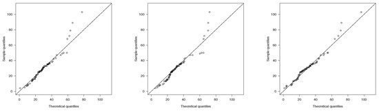
Figure 5. Q-Q plots in Neodymium dataset for: SBS model (left); MSBS model (middle); and GMSBS model (right)

5.2. Nickel Dataset

The descriptive summaries are given in Table 4. GMSBS, MSBS and SBS distributions are fitted to this dataset, the parameters are estimated via maximum likelihood (EM-algorithm), and their corresponding standard errors are given in parentheses in Table 5. The AIC values we obtained are given in Table 5. They suggest that GMSBS model provides the best fit to these data since this model exhibits less AIC.

Table 4. Summary of Nickel dataset.

n	$\overline{\mathit{t}}$	${\mathit{S}}_{\mathit{t}}$	${\mathit{g}}_1$	${\mathit{g}}_2$
85	21.59	16.5732	2.3922	11.325

Table 5. MLEs for Nickel dataset, their standard errors (in parenthesis) and AIC values.

Parameter	SBS	MSBS	GMSBS
$\alpha$	0.3877 (0.0918)	0.3266 (0.0852)	0.2490 (0.0330)
$\beta$	17.7982 (1.2464)	17.6017 (1.1027)	17.4961 (1.0622)
q	2.0118 (0.6967)	2.0932 (0.6284)	3.1927 (1.2341)
AIC	670.742	668.251	666.571

Figure 6 depicts the histogram for the data with the fitted density and the empirical cdf along with the cdf estimated by GMSBS model. QQ-plots are given in Figure 7. All of them show the good agreement of the GMSBS model for the Nickel data.

Figure 6. (left) Histogram of the Nickel data with estimated pdf of GMSBS distribution; and (right) empirical cdf (dotted lines) with estimated cdf of GMSBS model.

Figure 7. Q-Q plots in Nickel dataset for: SBS model (left); MSBS model (middle); and GMSBS model (right)

References

- Birnbaum, Z.W.; Saunders, S.C. A New Family of Life Distributions. J. Appl. Probab. 1969, 6, 319–327. [Google Scholar] [CrossRef]
- Birnbaum, Z.W.; Saunders, S.C. Estimation for a family of life distributions with applications to fatigue. J. Appl. Probab. 1969a, 6, 328–347. [Google Scholar] [CrossRef]
- Moors, J.J.A. A quantile alternative for kurtosis. J. R. Stat. Soc. Ser. D 1988, 37, 25–32. [Google Scholar] [CrossRef]
- Johnson, N.L.; Kotz, S.; Balakrishnan, N. Continuous Univariate Distributions, 2nd ed.; Wiley: New York, NY, USA, 1995; Volume 1. [Google Scholar]
- Leiva, V. The Birnbaum–Saunders Distribution; Academic Press: New York, NY, US, 2016. [Google Scholar]
- Gómez, H.W.; Olivares-Pacheco, J.F.; Bolfarine, H. An extension of the generalized Birnbaum–Saunders distribution. Stat. Probab. Lett. 2009, 79, 331–338. [Google Scholar] [CrossRef]
- Reyes, J.; Gómez, H.W.; Bolfarine, H. Modified slash distribution. Stat. J. Theor. App. Stat. 2013, 47, 929–941. [Google Scholar] [CrossRef]
- Rogers, W.H.; Tukey, J.W. Understanding some long-tailed symmetrical distributions. Stat. Neerl. 1972, 26, 211–226. [Google Scholar] [CrossRef]
- Reyes, J.; Barranco-Chamorro, I.; Gómez, H.W. Generalized modified slash distribution. 2018. Submitted. [Google Scholar]
- Abramowitz, M.; Stegun, I.A. Handbook of Mathematical Functions, 10th ed.; Handbook of Mathematical Functions: Dover, NY, USA, 1972. [Google Scholar]
- Reyes, J.; Vilca, F.; Gallardo, D.I.; Gómez, H.W. Modified slash Birnbaum–Saunders distribution. Hacettepe J. Math. Stat. Ser. B 2017, 46, 969–984. [Google Scholar] [CrossRef]
- Ng, H.; Kundu, D.; Balakrishnan, N. Modified moment estimation for the two-parameter Birnbaum–Saunders distribution. Comput. Stat. Data Anal. 2003, 43, 283–298. [Google Scholar] [CrossRef]
- Dempster, A.P.; Rubin, D.B.; Laird, N.M. Maximum likelihood from incomplete data via the EM algorithm (with discussion). J. R. Stat. Soc. B 1977, 39, 1–38. [Google Scholar]
- Lee, S.Y.; Xu, L. Influence analyses of nonlinear mixed-effects model. Comput. Stat. Data Anal. 2004, 45, 321–341. [Google Scholar] [CrossRef]
- Lin, X.S.; Liu, X. Markow aging process and phase-type law of mortality. N. Am. Actuar. J. 2007, 11, 92–109. [Google Scholar] [CrossRef]
- Akaike, H. A new look at the statistical model identification. IEEE Trans. Autom. Control 1974, 19, 716–723. [Google Scholar] [CrossRef]
- Rohatgi, V.K.; Ehsanes Saleh, A.K.M.D. An Introduction to Probability and Statistics, 3rd ed.; John Wiley and Sons: New York, NY, USA, 2001. [Google Scholar]
© 2018 by the authors. Licensee MDPI, Basel, Switzerland. This article is an open access article distributed under the terms and conditions of the Creative Commons Attribution (CC BY) license (http://creativecommons.org/licenses/by/4.0/).