Methods for Extracting Fractional Vegetation Cover from Differentiated Scenarios Based on Unmanned Aerial Vehicle Imagery

Abstract

Fractional vegetation cover (FVC) plays a key role in ecological and environmental status assessment because it directly reflects the extent of vegetation cover and its status, yet vegetation is an important component of ecosystems. FVC estimation methods have evolved from traditional manual interpretation to advanced remote sensing technologies, such as satellite data analysis and unmanned aerial vehicle (UAV) image processing. Extraction methods based on high-resolution UAV data are being increasingly studied in the fields of ecology and remote sensing. However, research on UAV-based FVC extraction against the backdrop of the high soil reflectance in arid regions remains scarce. In this paper, based on 12 UAV visible light images in differentiated scenarios in the Ebinur Lake basin, Xinjiang, China, various methods are used for high-precision FVC estimation: Otsu’s thresholding method combined with 12 Visible Vegetation Indices (abbreviated as Otsu-VVIs) (excess green index, excess red index, excess red minus green index, normalized green–red difference index, normalized green–blue difference index, red–green ratio index, color index of vegetation extraction, visible-band-modified soil-adjusted vegetation index, excess green minus red index, modified green–red vegetation index, red–green–blue vegetation index, visible-band difference vegetation index), color space method (red, green, blue, hue, saturation, value, lightness, ‘a’ (Green–Red component), and ‘b’ (Blue–Yellow component)), linear mixing model (LMM), and two machine learning algorithms (a support vector machine and a neural network). The results show that the following methods exhibit high accuracy in FVC extraction across differentiated scenarios: Otsu–CIVE, color space method (‘a’: Green–Red component), LMM, and SVM (Accuracy > 0.75, Precision > 0.8, kappa coefficient > 0.6). Nonetheless, higher scene complexity and image entropy reduce the applicability of precise FVC extraction methods. This study facilitates accurate, efficient extraction of vegetation information in differentiated scenarios within arid and semiarid regions, providing key technical references for FVC estimation in similar arid areas.

1. Introduction

Fractional vegetation cover (FVC), typically expressed as a percentage, represents the proportion of land surface covered by vegetation. It serves as a critical parameter for assessing vegetation health and understanding the interactions between global change and terrestrial ecosystems [1,2]. Moreover, FVC plays an essential role in evaluating ecosystem models and predicting ecological changes [3,4], highlighting its ecological, environmental, and societal relevance. Accurate FVC estimation aids in monitoring ecosystem health and contributes to the sustainable management of natural resources, essential for both environmental conservation and human society [5,6].

Arid and semiarid regions, such as Xinjiang, have distinctive ecosystems shaped by their unique geographical and climatic conditions. These regions are dominated by desert and grassland systems, where key vegetation types include desert plants like desert willow and poplar, semiarid species like bitterweed and reed, and mountain shrubs like saxaul and tamarisk [7,8,9]. These vegetation types play significant ecological roles, including mitigating wind erosion, preventing desertification, supporting wildlife habitats, and maintaining soil stability and water cycles. Given the ecological importance of this vegetation in Xinjiang, monitoring FVC is crucial for assessing regional ecological quality. However, traditional FVC retrieval methods face significant challenges due to environmental disturbances, necessitating the development of high-precision, repeatable techniques for accurate vegetation monitoring [10,11,12].

FVC extraction methods have traditionally relied on ground measurement and remote sensing. Ground-based methods, while precise, are resource-intensive and limited to small spatial and temporal scales, making them impractical in harsh environments [13,14]. Satellite remote sensing, on the other hand, provides wide coverage and allows large-scale vegetation monitoring, but its accuracy diminishes in arid and semiarid areas where vegetation is sparse and fragmented. The heterogeneity of these regions, coupled with complex terrain, further complicates satellite-based FVC extraction, and specialized methods are required for better accuracy [15,16].

In recent years, unmanned aerial vehicle (UAV) remote sensing has emerged as a promising alternative for estimating FVC, offering high spatial resolution, flexibility in data collection, and strong resistance to environmental interference [17,18]. Additionally, advances in machine learning algorithms have enhanced the ability to extract geoinformation from high-resolution UAV images, contributing to improved monitoring of vegetation dynamics and biodiversity [19,20]. Various techniques have been applied for FVC extraction, although the effectiveness of different algorithms varies depending on the region and vegetation characteristics [21,22].

This paper discusses different FVC extraction methods for arid and semiarid areas under varying entropy-difference conditions. The following Python-based methods are used: the Otsu–VVI method, color space method, linear mixing model [LMM], and two machine learning algorithms (a support vector machine [SVM] and a neural network [NN]). The precision of 24 extraction methods is validated using manually labeled points, confusion matrices, and kappa coefficients to select optimal algorithms suitable for arid and semiarid areas. This study aims to provide a scientific algorithmic basis and reference for the use of UAV monitoring in extracting FVC in such environments.

2. Materials

2.1. Study Area

The study area is in the Ebinur Lake basin, geographically situated between 43°38′ N and 45°52′ N, and 79°53′ E and 85°02′ E (Figure 1). The region features various geomorphological types, predominantly plains. Vegetation types are diverse and include the following: Saline vegetation: this vegetation dominates the area and is characterized by salt-tolerant plants. Common plants include Suaeda salsa and Haloxylon ammodendron [23], which are able to survive the saline conditions typical of the region. Wetland vegetation: this includes reedbeds dominated by Phragmites australis and Typha, which provide important habitat for waterfowl and act as natural water filters. Desert shrubs: in the surrounding arid areas, the vegetation includes drought-tolerant plants such as Tamarix chinensis Lour and Haloxylon ammodendron [24,25], which play an important role in stabilizing the soil and preventing erosion. Riparian vegetation: at the edge of the lake, plants such as Populus and Willow Salix provide important habitat for birds and other wildlife [26,27]. In recent years, human activities, especially agricultural expansion, irrigation water deployment and industrial development, dam construction, and pumping of water from water supply rivers have reduced the inflow to the lake, resulting in a drop in the water level and a drastic reduction in the size of the lake, a reduction which threatens biodiversity, especially the flora and fauna that depend on these ecosystems for their survival [28]. Changes in the Lake Ebey watershed therefore have important implications for scientific research and conservation efforts [29].

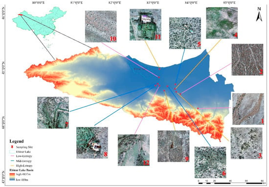
Figure 1. Overview map of the study area (the red numbers represent the number of each plot (1–12), and the different colored tows indicate the entropy values (high, medium, and low entropy) of the 12 plots).

2.2. UAV Data and Preprocessing

The UAV used in this study is the DJI Phantom4 RTK SE, which is equipped with a quadrotor flight system and a 20-million-pixel camera capable of capturing image information in three visible light bands (red: 650 nm ± 16 nm; green: 560 nm ± 16 nm; blue: 450 nm ± 16 nm [RGB]). The experiments were conducted from 28 July 2022 to 1 August 2022 using 3D photogrammetry (grid flight). The conditions were wind speeds less than 8 m/s, clear weather, visibility greater than 5 km, and a solar altitude angle greater than 45° at time of flight. The flight altitude was 40 m with an 80% lateral overlap and an 80% longitudinal overlap. Ground control points were established in each flight test site (total error < 0.5 m) to ensure the correct georegistration of UAV orthoimages (Figure 2). The collected UAV images were processed using the software Pix4D 4.4.10 (https://www.pix4d.com) (accessed on 11 July 2023) to obtain orthoimages with a pixel spatial resolution of 0.03 m. FVC was extracted from the UAV image data using a combination of methods based on Python: the Otsu–VVI method, the color space method, an LMM, and two machine learning algorithms (an SVM and an NN). These methods were evaluated for accuracy, and the optimal FVC extraction method was selected.

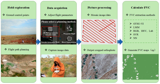
Figure 2. Flowchart of FVC extraction from UAV image data.

3. Methods

3.1. Scenarios and Entropy

Differentiated scenarios typically refer to specific environments influenced by varying geographic, climatic, and soil conditions and human activities. The concept of differentiated scenarios was used in this study to understand and analyze vegetation distribution and changes accurately under different environmental conditions. Based on manual visual interpretation, 12 orthorectified visible light (RGB) drone images obtained in the experiments were categorized into six scenarios according to vegetation distribution and surface complexity: (1) sparse shrub areas with similar backgrounds, (2) mixed grass–shrub areas with distinct ground vegetation demarcation, (3) mixed zone of sparse herbs and shrubs, (4) extensive shrub areas with minor grassland integration, (5) mixed grass–shrub areas with indistinguishable soil backgrounds, and (6) complex vegetation types with high cover and architectural interference.

Herein, entropy was used to describe these scenarios quantitatively. In remote sensing image processing, entropy is commonly used to measure the randomness or richness of information in image pixels [30]. Specifically for vegetation cover images, entropy can be used to analyze and differentiate the extent and type of vegetation coverage because different vegetation types and coverage exhibit various textures and gray-level variabilities. High entropy values indicate a wide and complex distribution of image pixel values, corresponding to areas with complex or mixed vegetation. Low entropy values suggest that the area is relatively uniform, with little variation in color and brightness, indicating simple vegetation areas. Entropy is typically calculated using a gray-level cooccurrence matrix (GLCM), a statistical method for characterizing image texture features [31]. A GLCM calculates the frequency distribution of gray-level similarity or dissimilarity between an image pixel and its neighboring pixels. Entropy is a statistical measure from this matrix used to describe the complexity and irregularity of image textures. The calculation formula is [31]

$$H=-{\sum }_{i=1}{p}_i{\mathit{log}}_2\left(p_i\right),$$

(1)

$$P_i=C_i/N,$$

(2)

where $P_i$ is the probability of the $i$th gray level occurring in the image, $C_i$ is the number of occurrences of gray level i, and $N$ is the total number of pixels in the image.

3.2. FVC Extraction Methods

(1)

Otsu–VVI Method

Otsu thresholding, also known as the maximum interclass variance method, is an adaptive thresholding method for image segmentation based on image data. Its principle involves calculating the image’s grayscale histogram to determine a threshold that divides the image into the foreground and background. VVIs (Table 1) are used to extract vegetation information from remote sensing images using the differential reflection between vegetation and nonvegetation areas [32,33]. These indices, typically calculated using visible light reflectance values, are based on data from different spectral bands [34]. Combining Otsu thresholding with VVIs leverages their respective advantages to enhance the accuracy and reliability of vegetation cover extraction.

Table 1. Visible Vegetation Indices (VVIs) and their formulas.

VVIs	Formula	Reference
Excess green index (EXG)	$2\times G-R-B$	[35]
Excess red index (EXR)	$1.4\times R-B$	[36]
Excess red minus green index (EXER)	$2\times G-2.4$	[37]
Normalized green–red difference index (NGRDI)	$(G-R)/(G+R)$	[38]
Normalized green–blue difference index (NGBDI)	$(G-B)/(G+B)$	[39]
Red–green ratio index (RGRI)	$R/B$	[40]
Visible-band difference vegetation index (VDVI)	$(2\times G-R-B)/(2\times G+R+B)$	[19]
Visible-band-modified soil-adjusted vegetation index (V-MSAVI)	$(2\times G+1-\sqrt{{\left(2\times G+1\right)}^2-8\times \left(2\times G-R-B\right)})/2$	[41]
Excess green minus red index (EXGR)	$3\times G-2.4\times R-B$	[42]
Modified green–red vegetation index (MGRVI)	$(G^2-R^2)/{(G}^2+R^2)$	[43]
Red–green–blue vegetation index (RGBVI)	$(G^2-\left(B\times R\right))/(G^2+\left(B\times R\right))$	[34]
Vegetation color index (CIVE)	$0.441\times R-0.811\times G+0.385\times B+18.78745$	[44]

R, G, and B represent the reflectance of the red, green, and blue bands, respectively.

(2)

Color Space Method

The color space method for FVC extraction is based on the absorption and reflection characteristics of vegetation at different wavelengths. This method involves converting color remote sensing images into an appropriate color space, commonly RGB; hue, saturation, value (HSV); and CIELab. Depending on the chosen color space, the original image is transformed into the corresponding color space, and the relevant color channels (R, G, B, H, S, V, L, a, and b) are extracted. Appropriate thresholds are set to segregate vegetated and nonvegetated areas within the image. Different color channels may require varying thresholds. Finally, FVC is obtained from UAV image data by calculating the proportion of vegetated pixels to nonvegetated ones in the binary image.

(3)

LMM

An LMM posits that the reflectance value of a pixel in a specific spectral band is a linear combination of the reflectance values of the pixel’s endmember components and their respective abundances [45].

$${Ref}_i={\sum }_{j=1}^m{P}_{i,j}+{\epsilon }_i$$

(3)

where $i=1,2,3,\dots ,n$ (where $n$ is the number of spectral bands); $j=\mathrm{1,2},3,\dots ,m$ (where $m$ is the number of endmember components within a pixel); ${Ref}_i$ is the mixed-pixel reflectance value; $P_{i,j}$ is the reflectance value of the $j$th endmember component in the $i$th spectral band; and ${\epsilon }_i$ is the error in the $i$th band.

(4)

SVM

An SVM fundamentally operates by identifying a hyperplane in the feature space that maximizes the margin between different classes. This hyperplane serves as a decision boundary that discriminates between classes. For data that are not linearly separable, an SVM uses kernel techniques to project these data into a higher-dimensional space to identify a linear separating hyperplane. An SVM solves the optimization problem [46]

$$\underset{w,b}{\min }{\displaystyle \frac{1}{2}}{‖w‖}^2+C{\sum }_{i=1}^n{\xi }_i$$

(4)

subject to the constraints

$$y_i(w·x_i+b)\ge 1-{\xi }_i, { \xi }_i\ge 0, i=1,\dots ,n,$$

(5)

where $w$ is the normal vector to the hyperplane; $b$ is the bias of the hyperplane; $C$ is a regularization parameter that controls the misclassification penalty; ${\xi }_i$ denotes slack variables, allowing some data points to be on the incorrect side of the margin; $y_i$ is the label of each sample, typically +1 or −1; and $x_i$ denotes the feature vectors.

The SVM model parameter settings include the kernel type, penalty coefficient $C$, and gamma. $C$ balances the accuracy of classification with the smoothness of the decision surface. A larger $C$ can reduce training errors but may lead to overfitting, whereas a smaller $C$ enhances the model’s robustness to noise but may increase training errors. The gamma parameter determines the reach of a single training example’s influence, thereby affecting classification granularity or smoothness.

(5)

NN

Numerous nodes (neurons) are organized in a hierarchical structure within an NN. Each neuron processes input signals through an activation function and produces output signals for the next layer. In an NN, each connection has a weight, which is adjusted during training through backpropagation algorithms to minimize the error between the model outputs and the true labels. The basic equations of an NN involve forward propagation and error backpropagation processes. In forward propagation, the output $y$ of each neuron is calculated as [36]

$$y=f\left({\sum }_{i=1}^n{w}_i{x}_i+b\right),$$

(6)

where $x_i$ is the input value; $w_i$ is the weight; $b$ is the bias; and $f$ is the activation function, whose common functions include sigmoid, tanh, or ReLU. During backpropagation, the network minimizes the loss function, typically a function of the prediction error, such as the mean squared error or cross-entropy loss.

The number of hidden layers and nodes, activation function, learning rate, number of epochs, and batch size are commonly used parameters in traditional MLP NNs. The numbers of hidden layers and their nodes define the network depth and width, respectively, with each hidden layer potentially having a distinct number of nodes. Additional layers and nodes can increase model complexity and lead to overfitting. Common activation functions include sigmoid, tanh, and ReLU, which introduce nonlinear factors allowing the network to learn complex data patterns. The learning rate, which determines the step size of weight adjustments, is a crucial parameter in optimization algorithms. The number of iterations, or epochs, is the number of times the entire training dataset is used to update the model weights, with multiple iterations helping the network learn better. During training, data are divided into batches, each used to compute model errors and update weights.

3.3. Precision Evaluation

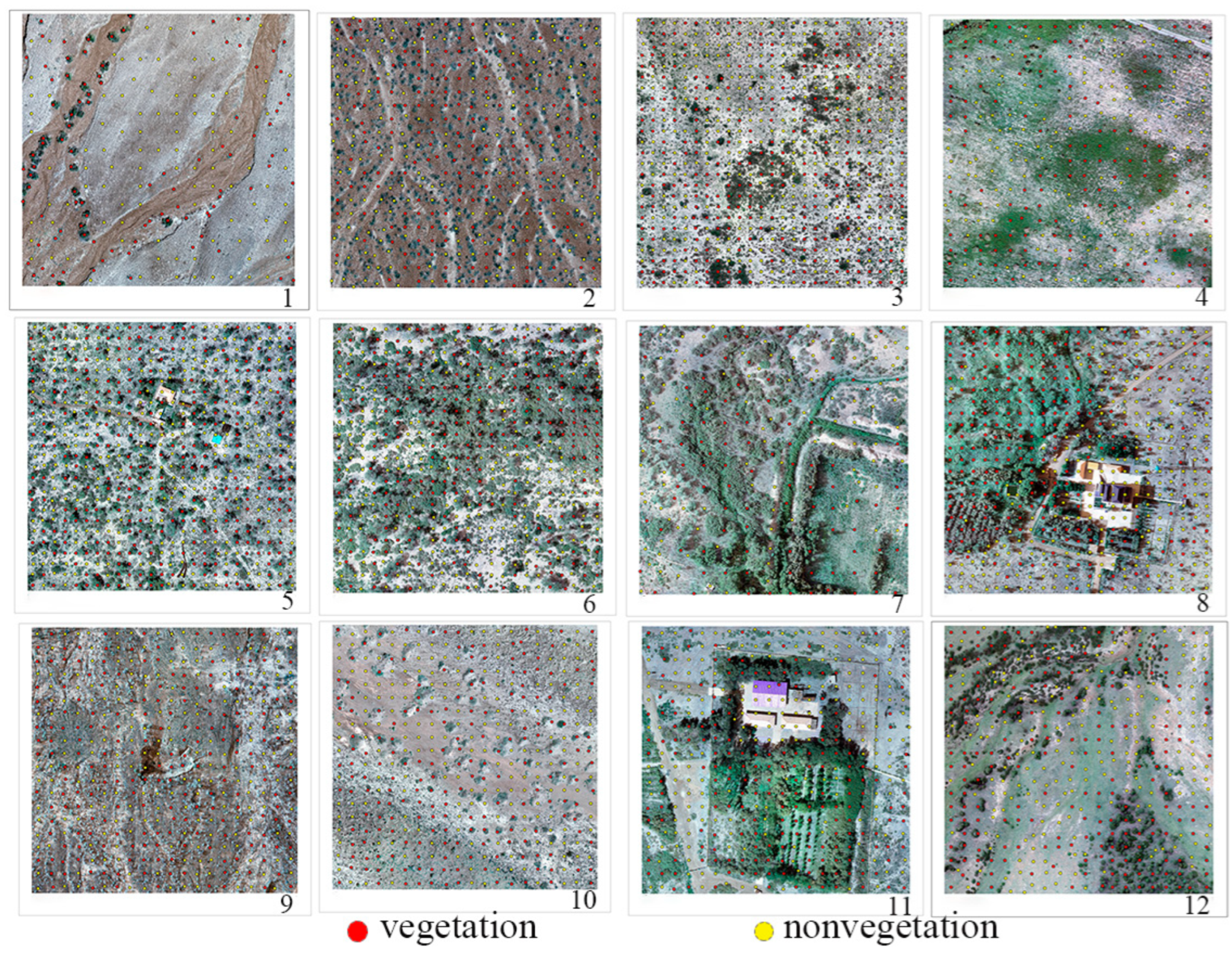
The vegetated and nonvegetated areas in the 12 UAV images were manually marked in this study (Figure 3). According to the area size and vegetation sparsity, type, and complexity, vegetation and nonvegetation were proportionally marked in the images. From the 1st image to the 12th image, named 1–12, the total number of point markers was 200, 400, 600, 300, 600, 500, 200, 500, 400, 400, and 400, respectively. The 12 marked images were then used to extract vegetation cover using the Otsu–VVI method, color space method, LMM, and two machine learning methods (SVM and NN), followed by accuracy validation using confusion matrices and kappa coefficients.

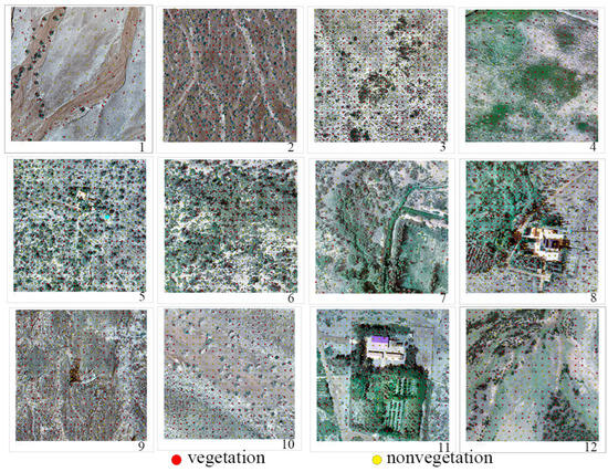
Figure 3. Thumbnails of 12 markers.

(1)

Confusion Matrix

The FVC extraction results of different methods were evaluated using confusion matrices and accuracy metrics [37] (Formulas (7)–(12); Table 2).

$$Accuracy={\displaystyle \frac{a+d}{a+b+c+d}}$$

(7)

$$Precision={\displaystyle \frac{a}{a+c}}$$

(8)

$$Recall={\displaystyle \frac{a}{a+b}}$$

(9)

$$f={\displaystyle \frac{2a}{2a+b+c}}$$

(10)

$$OA={\displaystyle \frac{c}{c+d}}$$

(11)

$$UA={\displaystyle \frac{b}{a+b}}$$

(12)

Table 2. Confusion matrix for precision validation.

Marking Result	Extraction Result
	FVC	non-FVC
FVC	a	b
non-FVC	c	d

Several key statistical metrics were used to assess the FVC extraction accuracy of the classification models: total accuracy, precision, recall, overestimation error, underestimation error, and the $f$ score. These metrics are defined as follows:

$Accuracy$: This is the proportion of correctly identified observations (vegetation and nonvegetation in this study) to the total number of observations. This is the most straightforward performance evaluation metric; a higher value indicates better overall model performance.

$Precision$: This was the proportion of correctly predicted vegetation observations out of all predicted vegetation. A higher value indicated higher accuracy in the predicted vegetation samples.

$Recall$: This metric was the proportion of actual vegetation observations that were correctly predicted as vegetation. A higher value indicated a stronger ability of the model to extract vegetation.

$f$ score: This is the harmonic mean of precision and recall, ranging between 0 and 1. Values closer to 1 indicated better FVC extraction effectiveness.

Overestimation Error ($OA$): This metric was the probability of nonvegetation observations being incorrectly predicted as vegetation.

$N$ is the total number of observations, $X$ is the number of correct classifications, and $E$ is the number expected by chance. The kappa coefficient ranges from −1 (total disagreement) to +1 (perfect agreement); a value of 0 indicates that the observed agreement is random. In practical applications, a higher kappa value signifies better classification performance and considers the impact of random factors.

Underestimation Error ($UA$): This refers to the probability of vegetation observations being missed or undetected.

These metrics constitute a comprehensive framework for evaluating the performance of vegetation classification models in different aspects. Total accuracy reflects the overall accuracy of each model. Underestimation and overestimation errors provide information about potential misjudgments by each model.

(2)

Kappa Coefficient

The kappa coefficient is a statistical measure used to assess classification accuracy, especially in terms of accounting for random agreement. In the classification of FVC, the kappa coefficient was used to understand the degree of consistency between the classification results and actual conditions, providing insights beyond those offered by overall accuracy alone. The kappa coefficient of each FVC extraction method was calculated as [38]

$$N=a+b+c+d,$$

(13)

$$X=a+d,$$

(14)

$$E=\left({\displaystyle \frac{(a+c)\times (a+b)}{N}}\right)+\left({\displaystyle \frac{(b+d)\times (c+b)}{N}}\right),$$

(15)

$$Kappa={\displaystyle \frac{X-E}{N-E}}.$$

(16)

4. Result

4.1. Scenarios and Entropy

Entropy values were calculated for the 12 images across the six scenarios (Table 3). Based on the average entropy value and standard deviation, entropy classifications were assigned as follows: high entropy (values greater than the mean minus 0.5 times the standard deviation), low entropy (values less than the mean minus 0.5 times the standard deviation), and medium entropy (values in between). These categories were used to classify each of the 12 images into low-, medium-, and high-entropy categories. Subsequently, FVC was extracted from these images using the Otsu–VVI method, color space method, LMM, SVM, and NN.

Table 3. Classification of entropy and differentiated scenarios.

No.	Entropy	Differentiated Scenario
1	Low Entropy	Sparse shrub areas with similar backgrounds
2	Low Entropy	Sparse shrub areas with similar backgrounds
3	Medium Entropy	Mixed grass–shrub areas with distinct ground vegetation demarcation
4	Medium Entropy	Areas cooccupied by shrubs and sparse herbaceous vegetation
5	High Entropy	Complex vegetation types with high cover and architectural interference
6	High Entropy	Extensive shrub areas with minor grassland integration
7	High Entropy	Extensive shrub areas with minor grassland integration
8	High Entropy	Complex vegetation types with high cover and architectural interference
9	Medium Entropy	Mixed grass–shrub areas with indistinguishable soil backgrounds
10	Low Entropy	Mixed grass–shrub areas with distinct ground vegetation demarcation
11	Medium Entropy	Complex vegetation types with high cover and architectural interference
12	Low Entropy	Areas cooccupied by shrubs and sparse herbaceous vegetation

High entropy > Mean-0.5 × SD; low entropy < Mean-0.5 × SD; Mean-0.5 × SD ≤ medium entropy ≤ Mean: 0.5 × SD, where SD is the standard deviation and Mean is the mean.

4.2. Otsu–VVIs

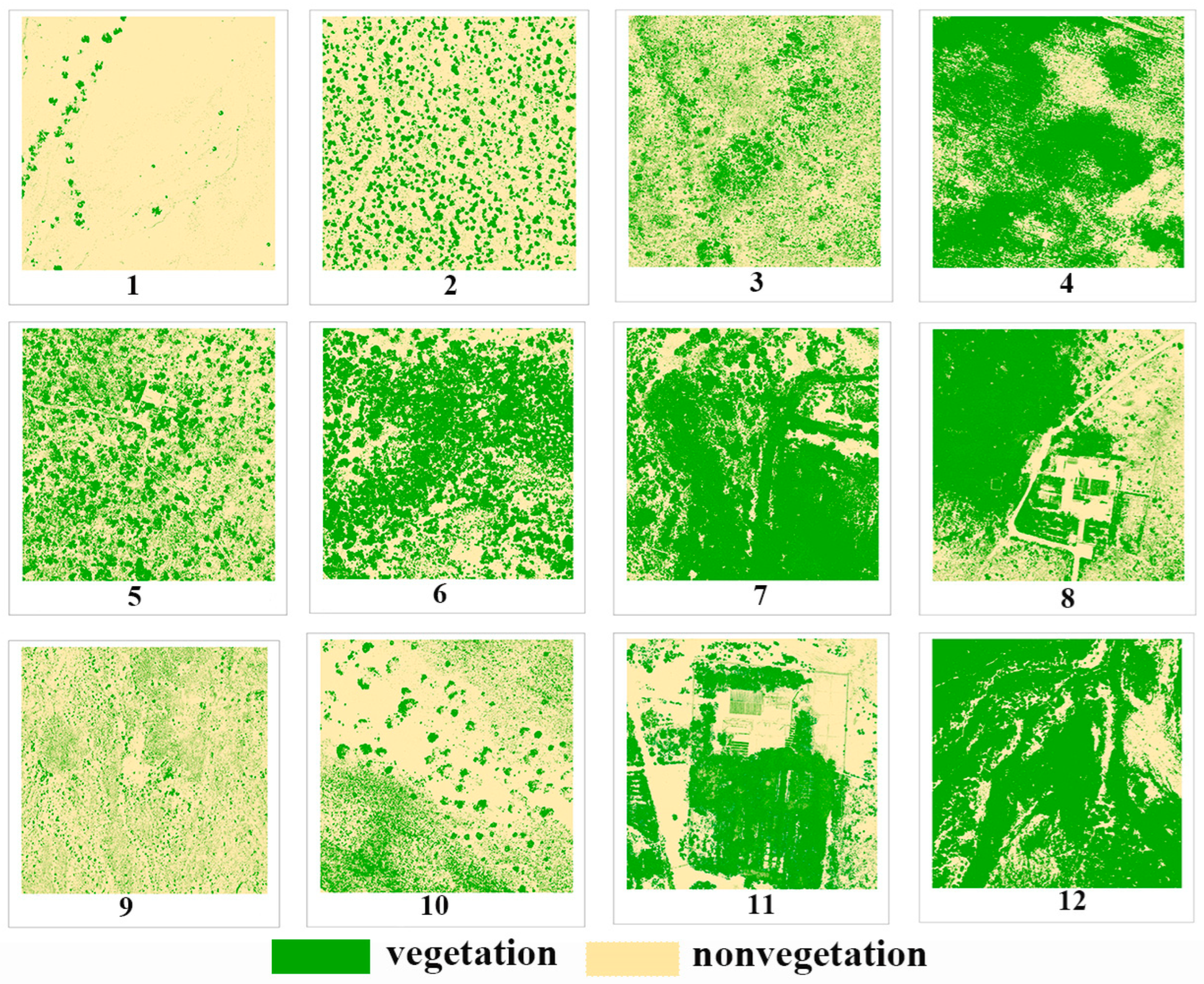
Twelve Otsu–VVI methods were used to extract FVC from the 12 orthorectified RGB drone images, and extraction result maps were generated (Figure 4; Table 4).

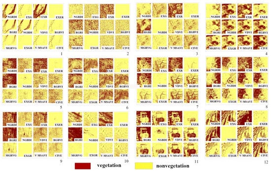
Figure 4. Thumbnails of 12 UAV results extracted based on the Otsu–VVI method.

Table 4. Accuracy verification of Otsu–VVI method ^a.

No.	VVIs	$\mathbf{a}$	$\mathbf{b}$	$\mathbf{c}$	$\mathbf{d}$	$\mathbf{A}\mathbf{c}\mathbf{c}\mathbf{u}\mathbf{r}\mathbf{a}\mathbf{c}\mathbf{y}$	$\mathbf{P}\mathbf{r}\mathbf{e}\mathbf{c}\mathbf{i}\mathbf{s}\mathbf{i}\mathbf{o}\mathbf{n}$	$\mathbf{R}\mathbf{e}\mathbf{c}\mathbf{a}\mathbf{l}\mathbf{l}$	$\mathbf{f}$	$\mathbf{O}\mathbf{A}$	$\mathbf{U}\mathbf{A}$
1	NGRDI	61	39	79	21	0.410	0.436	0.610	0.508	0.790	0.390
	EXG	63	37	3	97	0.800	0.955	0.630	0.759	0.030	0.370
	EXR	37	63	59	41	0.390	0.385	0.370	0.378	0.590	0.630
	EXER	0	100	0	100	0.500	0.000	0.000	0.000	0.000	1.000
	RGRI	69	31	92	8	0.385	0.429	0.690	0.529	0.920	0.310
	NGBDI	2	98	11	89	0.455	0.154	0.020	0.035	0.110	0.980
	VDVI	68	32	2	98	0.830	0.971	0.680	0.800	0.020	0.320
	RGBVI	61	39	1	99	0.800	0.984	0.610	0.753	0.010	0.390
	MGRVI	21	79	3	97	0.590	0.875	0.210	0.339	0.030	0.790
	EXGR	2	98	0	100	0.510	1.000	0.020	0.039	0.000	0.980
	V-MSAVI	59	41	1	99	0.790	0.983	0.590	0.738	0.010	0.410
	CIVE	69	31	4	96	0.825	0.945	0.690	0.798	0.040	0.310
2	NGRDI	68	132	2	198	0.665	0.971	0.340	0.504	0.010	0.660
	EXG	126	74	23	177	0.758	0.846	0.630	0.722	0.115	0.370
	EXR	163	37	79	121	0.710	0.674	0.815	0.738	0.395	0.185
	EXER	0	200	0	200	0.500	0.000	0.000	0.000	0.000	1.000
	RGRI	159	41	46	154	0.783	0.776	0.795	0.785	0.230	0.205
	NGBDI	5	195	94	106	0.278	0.051	0.025	0.033	0.470	0.975
	VDVI	126	74	14	186	0.780	0.900	0.630	0.741	0.070	0.370
	RGBVI	127	73	15	185	0.780	0.894	0.635	0.743	0.075	0.365
	MGRVI	5	195	90	110	0.288	0.053	0.025	0.034	0.450	0.975
	EXGR	0	200	0	200	0.500	0.000	0.000	0.000	0.000	1.000
	V-MSAVI	125	75	14	186	0.778	0.899	0.625	0.737	0.070	0.375
	CIVE	138	62	30	170	0.770	0.821	0.690	0.750	0.150	0.310
3	NGRDI	34	266	24	276	0.517	0.586	0.113	0.190	0.080	0.887
	EXG	177	123	2	298	0.792	0.989	0.590	0.739	0.007	0.410
	EXR	43	257	295	5	0.080	0.127	0.143	0.135	0.983	0.857
	EXER	15	285	0	300	0.525	1.000	0.050	0.095	0.000	0.950
	RGRI	70	230	156	144	0.357	0.310	0.233	0.266	0.520	0.767
	NGBDI	0	300	0	300	0.500	0.000	0.000	0.000	0.000	1.000
	VDVI	153	147	2	298	0.752	0.987	0.510	0.673	0.007	0.490
	RGBVI	168	132	2	298	0.777	0.988	0.560	0.715	0.007	0.440
	MGRVI	121	179	1	299	0.700	0.992	0.403	0.573	0.003	0.597
	EXGR	59	241	1	299	0.597	0.983	0.197	0.328	0.003	0.803
	V-MSAVI	171	129	2	298	0.782	0.988	0.570	0.723	0.007	0.430
	CIVE	186	114	2	298	0.807	0.989	0.620	0.762	0.007	0.380
4	NGRDI	4	146	47	103	0.357	0.078	0.027	0.040	0.313	0.973
	EXG	111	39	0	150	0.870	1.000	0.740	0.851	0.000	0.260
	EXR	44	106	148	2	0.153	0.229	0.293	0.257	0.987	0.707
	EXER	41	109	150	150	0.424	0.215	0.273	0.240	0.500	0.727
	RGRI	12	138	108	42	0.180	0.100	0.080	0.089	0.720	0.920
	NGBDI	98	52	0	150	0.827	1.000	0.653	0.790	0.000	0.347
	VDVI	96	54	0	150	0.820	1.000	0.640	0.780	0.000	0.360
	RGBVI	104	46	0	150	0.847	1.000	0.693	0.819	0.000	0.307
	MGRVI	90	60	0	150	0.800	1.000	0.600	0.750	0.000	0.400
	EXGR	80	70	0	150	0.767	1.000	0.533	0.696	0.000	0.467
	V-MSAVI	109	41	0	150	0.863	1.000	0.727	0.842	0.000	0.273
	CIVE	133	17	0	150	0.943	1.000	0.887	0.940	0.000	0.113
5	NGRDI	89	211	157	143	0.387	0.362	0.297	0.326	0.523	0.703
	EXG	196	104	3	297	0.822	0.985	0.653	0.786	0.010	0.347
	EXR	118	181	291	9	0.212	0.289	0.395	0.333	0.970	0.605
	EXER	3	297	1	299	0.503	0.750	0.010	0.020	0.003	0.990
	RGRI	126	174	264	36	0.270	0.323	0.420	0.365	0.880	0.580
	NGBDI	1	299	4	296	0.495	0.200	0.003	0.007	0.013	0.997
	VDVI	173	127	2	298	0.785	0.989	0.577	0.728	0.007	0.423
	RGBVI	179	121	2	298	0.795	0.989	0.597	0.744	0.007	0.403
	MGRVI	105	195	3	297	0.670	0.972	0.350	0.515	0.010	0.650
	EXGR	51	249	1	299	0.583	0.981	0.170	0.290	0.003	0.830
	V-MSAVI	183	117	2	298	0.802	0.989	0.610	0.755	0.007	0.390
	CIVE	208	92	4	296	0.840	0.981	0.693	0.813	0.013	0.307
6	NGRDI	43	207	43	62	0.296	0.500	0.172	0.256	0.410	0.828
	EXG	175	75	0	250	0.850	1.000	0.700	0.824	0.000	0.300
	EXR	109	141	228	22	0.262	0.323	0.436	0.371	0.912	0.564
	EXER	6	244	0	250	0.512	1.000	0.024	0.047	0.000	0.976
	RGRI	67	183	238	12	0.158	0.220	0.268	0.241	0.952	0.732
	NGBDI	3	247	12	238	0.482	0.200	0.012	0.023	0.048	0.988
	VDVI	158	92	0	250	0.816	1.000	0.632	0.775	0.000	0.368
	RGBVI	162	88	0	250	0.824	1.000	0.648	0.786	0.000	0.352
	MGRVI	83	167	0	250	0.666	1.000	0.332	0.498	0.000	0.668
	EXGR	37	213	0	250	0.574	1.000	0.148	0.258	0.000	0.852
	V-MSAVI	168	82	0	250	0.836	1.000	0.672	0.804	0.000	0.328
	CIVE	188	62	0	250	0.876	1.000	0.752	0.858	0.000	0.248
7	NGRDI	10	90	67	33	0.215	0.130	0.100	0.113	0.670	0.900
	EXG	53	47	1	99	0.760	0.981	0.530	0.688	0.010	0.470
	EXR	64	36	80	20	0.420	0.444	0.640	0.525	0.800	0.360
	EXER	5	95	0	100	0.525	1.000	0.050	0.095	0.000	0.950
	RGRI	16	84	87	13	0.145	0.155	0.160	0.158	0.870	0.840
	NGBDI	0	100	6	94	0.470	0.000	0.000	0.000	0.060	1.000
	VDVI	50	50	1	99	0.745	0.980	0.500	0.662	0.010	0.500
	RGBVI	52	48	1	99	0.755	0.981	0.520	0.680	0.010	0.480
	MGRVI	24	76	0	100	0.620	1.000	0.240	0.387	0.000	0.760
	EXGR	20	80	0	100	0.600	1.000	0.200	0.333	0.000	0.800
	V-MSAVI	56	44	1	99	0.775	0.982	0.560	0.713	0.010	0.440
	CIVE	73	27	1	99	0.860	0.986	0.730	0.839	0.010	0.270
8	NGRDI	30	220	155	95	0.250	0.162	0.120	0.138	0.620	0.880
	EXG	147	103	1	249	0.792	0.993	0.588	0.739	0.004	0.412
	EXR	149	101	186	64	0.426	0.445	0.596	0.509	0.744	0.404
	EXER	36	214	13	237	0.546	0.735	0.144	0.241	0.052	0.856
	RGRI	44	206	193	57	0.202	0.186	0.176	0.181	0.772	0.824
	NGBDI	4	246	47	203	0.414	0.078	0.016	0.027	0.188	0.984
	VDVI	163	87	2	248	0.822	0.988	0.652	0.786	0.008	0.348
	RGBVI	152	98	2	248	0.800	0.987	0.608	0.752	0.008	0.392
	MGRVI	73	177	32	218	0.582	0.695	0.292	0.411	0.128	0.708
	EXGR	64	186	1	249	0.626	0.985	0.256	0.406	0.004	0.744
	V-MSAVI	164	86	2	248	0.824	0.988	0.656	0.788	0.008	0.344
	CIVE	183	67	3	247	0.860	0.984	0.732	0.839	0.012	0.268
9	NGRDI	179	21	89	111	0.725	0.668	0.895	0.765	0.445	0.105
	EXG	153	47	23	177	0.825	0.869	0.765	0.814	0.115	0.235
	EXR	187	13	88	112	0.748	0.680	0.935	0.787	0.440	0.065
	EXER	0	200	1	199	0.498	0.000	0.000	0.000	0.005	1.000
	RGRI	191	9	140	60	0.628	0.577	0.955	0.719	0.700	0.045
	NGBDI	0	200	47	153	0.383	0.000	0.000	0.000	0.235	1.000
	VDVI	170	30	45	155	0.813	0.791	0.850	0.819	0.225	0.150
	RGBVI	160	40	3	197	0.893	0.982	0.800	0.882	0.015	0.200
	MGRVI	4	196	23	177	0.453	0.148	0.020	0.035	0.115	0.980
	EXGR	2	198	0	200	0.505	1.000	0.010	0.020	0.000	0.990
	V-MSAVI	150	50	3	197	0.868	0.980	0.750	0.850	0.015	0.250
	CIVE	142	58	9	191	0.833	0.940	0.710	0.809	0.045	0.290
10	NGRDI	20	180	62	138	0.395	0.244	0.100	0.142	0.310	0.900
	EXG	182	18	1	199	0.953	0.995	0.910	0.950	0.005	0.090
	EXR	102	98	119	81	0.458	0.462	0.510	0.485	0.595	0.490
	EXER	0	200	0	200	0.500	0.000	0.000	0.000	0.000	1.000
	RGRI	53	147	181	19	0.180	0.226	0.265	0.244	0.905	0.735
	NGBDI	1	199	10	190	0.478	0.091	0.005	0.009	0.050	0.995
	VDVI	184	16	1	199	0.958	0.995	0.920	0.956	0.005	0.080
	RGBVI	181	19	1	199	0.950	0.995	0.905	0.948	0.005	0.095
	MGRVI	94	106	1	199	0.733	0.989	0.470	0.637	0.005	0.530
	EXGR	34	166	200	200	0.390	0.145	0.170	0.157	0.500	0.830
	V-MSAVI	183	17	1	199	0.955	0.995	0.915	0.953	0.005	0.085
	CIVE	189	11	2	198	0.968	0.990	0.945	0.967	0.010	0.055
11	NGRDI	26	174	154	46	0.180	0.144	0.130	0.137	0.770	0.870
	EXG	125	75	1	199	0.810	0.992	0.625	0.767	0.005	0.375
	EXR	47	153	175	25	0.180	0.212	0.235	0.223	0.875	0.765
	EXER	20	180	1	199	0.548	0.952	0.100	0.181	0.005	0.900
	RGRI	29	171	180	20	0.123	0.139	0.145	0.142	0.900	0.855
	NGBDI	0	200	18	182	0.455	0.000	0.000	0.000	0.090	1.000
	VDVI	128	72	1	199	0.818	0.992	0.640	0.778	0.005	0.360
	RGBVI	124	76	1	199	0.808	0.992	0.620	0.763	0.005	0.380
	MGRVI	87	113	4	196	0.708	0.956	0.435	0.598	0.020	0.565
	EXGR	49	151	1	199	0.620	0.980	0.245	0.392	0.005	0.755
	V-MSAVI	142	58	1	199	0.853	0.993	0.710	0.828	0.005	0.290
	CIVE	167	33	9	191	0.895	0.949	0.835	0.888	0.045	0.165
12	NGRDI	40	160	126	74	0.285	0.241	0.200	0.219	0.630	0.800
	EXG	121	79	7	193	0.785	0.945	0.605	0.738	0.035	0.395
	EXR	111	89	190	10	0.303	0.369	0.555	0.443	0.950	0.445
	EXER	16	184	0	200	0.540	1.000	0.080	0.148	0.000	0.920
	RGRI	73	127	167	33	0.265	0.304	0.365	0.332	0.835	0.635
	NGBDI	0	200	5	195	0.488	0.000	0.000	0.000	0.025	1.000
	VDVI	79	121	0	200	0.698	1.000	0.395	0.566	0.000	0.605
	RGBVI	78	122	0	200	0.695	1.000	0.390	0.561	0.000	0.610
	MGRVI	62	138	0	200	0.655	1.000	0.310	0.473	0.000	0.690
	EXGR	39	161	0	200	0.598	1.000	0.195	0.326	0.000	0.805
	V-MSAVI	88	112	0	200	0.720	1.000	0.440	0.611	0.000	0.560
	CIVE	133	67	6	194	0.818	0.957	0.665	0.785	0.030	0.335

^a a, b, c, and d in the Table 4 header indicate extracted results and results made from the confusion matrix.

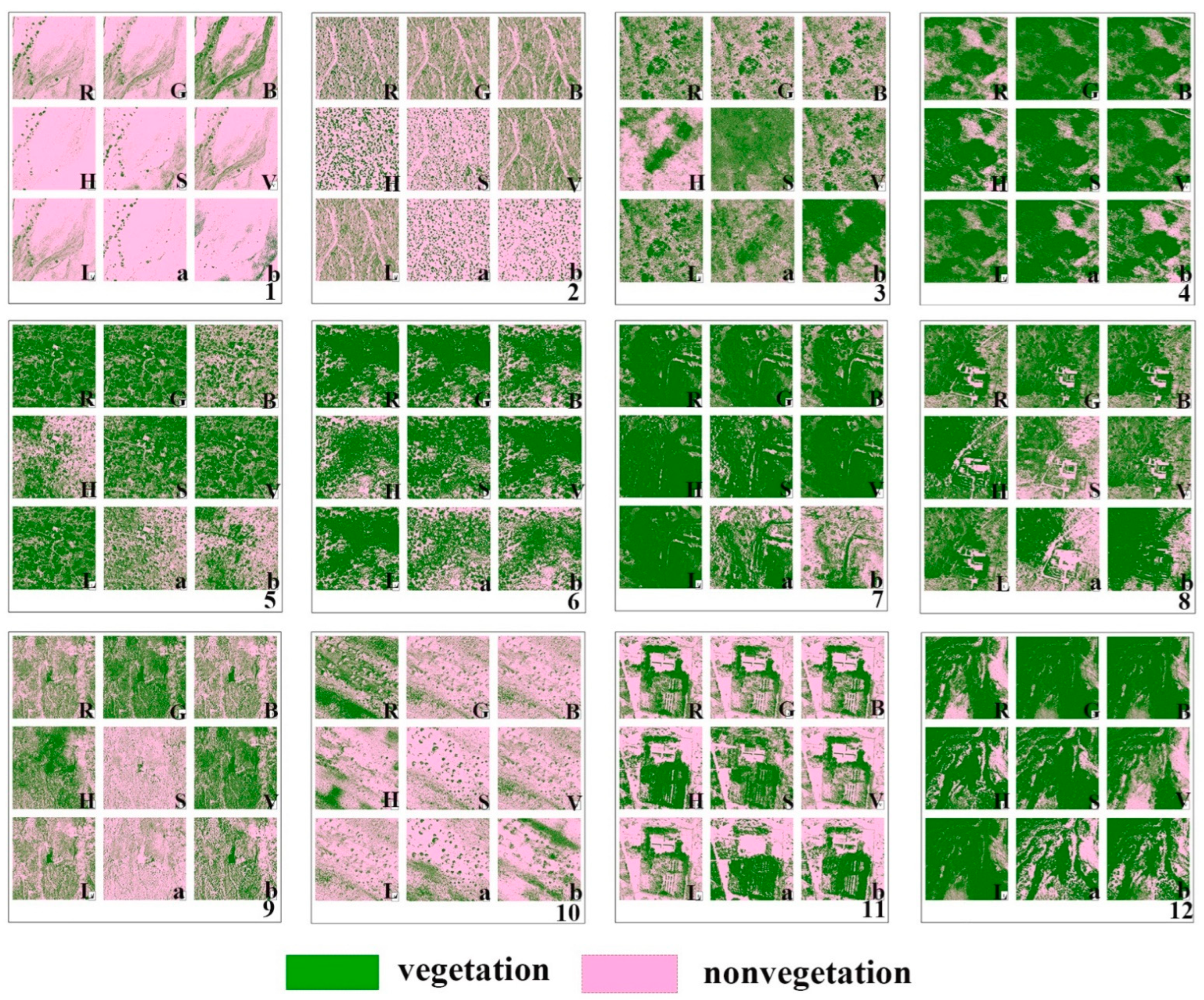
4.3. Color Space Method

FVC was extracted from the 12 images using the color space method, and FVC extraction result maps were produced (Figure 5; Table 5).

Figure 5. Thumbnails of 12 UAV image results extracted based on the color space method. R, G, B, H, S, V, L, a and b in Figure 5 represent the components in the color space method, respectively.

Table 5. Accuracy verification of color space method ^a.

No.	Component	$\mathbf{a}$	$\mathbf{b}$	$\mathbf{c}$	$\mathbf{d}$	$\mathbf{A}\mathbf{c}\mathbf{c}\mathbf{u}\mathbf{r}\mathbf{a}\mathbf{c}\mathbf{y}$	$\mathbf{P}\mathbf{r}\mathbf{e}\mathbf{c}\mathbf{i}\mathbf{s}\mathbf{i}\mathbf{o}\mathbf{n}$	$\mathbf{R}\mathbf{e}\mathbf{c}\mathbf{a}\mathbf{l}\mathbf{l}$	$\mathbf{f}$	$\mathbf{O}\mathbf{A}$	$\mathbf{U}\mathbf{A}$
1	R	94	6	30	70	0.820	0.758	0.940	0.839	0.300	0.060
	G	76	24	31	69	0.725	0.710	0.760	0.734	0.310	0.240
	B	69	31	30	70	0.695	0.697	0.690	0.693	0.300	0.310
	H	35	65	5	95	0.650	0.875	0.350	0.500	0.050	0.650
	S	63	37	7	93	0.780	0.900	0.630	0.741	0.070	0.370
	V	40	60	8	92	0.660	0.833	0.400	0.541	0.080	0.600
	L	43	57	10	90	0.665	0.811	0.430	0.562	0.100	0.570
	a	72	28	3	97	0.845	0.960	0.720	0.823	0.030	0.280
	b	21	79	9	91	0.560	0.700	0.210	0.323	0.090	0.790
2	R	155	45	45	155	0.775	0.775	0.775	0.775	0.225	0.225
	G	124	76	58	142	0.665	0.681	0.620	0.649	0.290	0.380
	B	111	89	64	136	0.618	0.634	0.555	0.592	0.320	0.445
	H	183	17	9	191	0.935	0.953	0.915	0.934	0.045	0.085
	S	155	45	20	180	0.838	0.886	0.775	0.827	0.100	0.225
	V	131	69	59	141	0.680	0.689	0.655	0.672	0.295	0.345
	L	123	77	50	150	0.683	0.711	0.615	0.660	0.250	0.385
	a	158	42	14	186	0.860	0.919	0.790	0.849	0.070	0.210
	b	130	70	5	195	0.813	0.963	0.650	0.776	0.025	0.350
3	R	297	3	5	295	0.987	0.983	0.990	0.987	0.017	0.010
	G	285	15	3	297	0.970	0.990	0.950	0.969	0.010	0.050
	B	282	18	3	297	0.965	0.989	0.940	0.964	0.010	0.060
	H	156	144	92	208	0.607	0.629	0.520	0.569	0.307	0.480
	S	246	54	253	47	0.488	0.493	0.820	0.616	0.843	0.180
	V	293	7	7	293	0.977	0.977	0.977	0.977	0.023	0.023
	L	296	4	10	190	0.972	0.967	0.987	0.977	0.050	0.013
	a	282	18	92	208	0.817	0.754	0.940	0.837	0.307	0.060
	b	246	54	225	75	0.535	0.522	0.820	0.638	0.750	0.180
4	R	131	19	2	148	0.930	0.985	0.873	0.926	0.013	0.127
	G	140	10	4	146	0.953	0.972	0.933	0.952	0.027	0.067
	B	138	12	2	148	0.953	0.986	0.920	0.952	0.013	0.080
	H	138	12	36	114	0.840	0.793	0.920	0.852	0.240	0.080
	S	138	12	5	145	0.943	0.965	0.920	0.942	0.033	0.080
	V	138	12	4	146	0.947	0.972	0.920	0.945	0.027	0.080
	L	139	11	3	147	0.953	0.979	0.927	0.952	0.020	0.073
	a	139	11	5	145	0.947	0.965	0.927	0.946	0.033	0.073
	b	133	17	32	118	0.837	0.806	0.887	0.844	0.213	0.113
5	R	293	7	16	284	0.962	0.948	0.977	0.962	0.053	0.023
	G	292	8	15	285	0.962	0.951	0.973	0.962	0.050	0.027
	B	260	40	11	289	0.915	0.959	0.867	0.911	0.037	0.133
	H	236	64	91	209	0.742	0.722	0.787	0.753	0.303	0.213
	S	260	40	19	281	0.902	0.932	0.867	0.898	0.063	0.133
	V	291	9	14	286	0.962	0.954	0.970	0.962	0.047	0.030
	L	293	7	14	286	0.965	0.954	0.977	0.965	0.047	0.023
	a	242	58	6	294	0.893	0.976	0.807	0.883	0.020	0.193
	b	193	107	28	272	0.775	0.873	0.643	0.741	0.093	0.357
6	R	246	4	59	191	0.874	0.807	0.984	0.886	0.236	0.016
	G	246	4	55	195	0.882	0.817	0.984	0.893	0.220	0.016
	B	227	23	25	225	0.904	0.901	0.908	0.904	0.100	0.092
	H	221	29	39	211	0.864	0.850	0.884	0.867	0.156	0.116
	S	226	24	86	164	0.780	0.724	0.904	0.804	0.344	0.096
	V	247	3	43	207	0.908	0.852	0.988	0.915	0.172	0.012
	L	246	4	45	205	0.902	0.845	0.984	0.909	0.180	0.016
	a	214	36	8	242	0.912	0.964	0.856	0.907	0.032	0.144
	b	192	58	35	215	0.814	0.846	0.768	0.805	0.140	0.232
7	R	97	3	38	62	0.795	0.719	0.970	0.826	0.380	0.030
	G	93	7	38	62	0.775	0.710	0.930	0.805	0.380	0.070
	B	93	7	32	68	0.805	0.744	0.930	0.827	0.320	0.070
	H	95	5	28	72	0.835	0.772	0.950	0.852	0.280	0.050
	S	96	4	35	65	0.805	0.733	0.960	0.831	0.350	0.040
	V	98	2	53	47	0.725	0.649	0.980	0.781	0.530	0.020
	L	98	2	58	42	0.700	0.628	0.980	0.766	0.580	0.020
	a	94	6	12	88	0.910	0.887	0.940	0.913	0.120	0.060
	b	54	46	19	81	0.675	0.740	0.540	0.624	0.190	0.460
8	R	211	39	110	140	0.702	0.657	0.844	0.739	0.440	0.156
	G	210	40	105	145	0.710	0.667	0.840	0.743	0.420	0.160
	B	216	34	216	127	0.578	0.500	0.864	0.633	0.630	0.136
	H	242	8	250	0	0.484	0.492	0.968	0.652	1.000	0.032
	S	172	78	250	0	0.344	0.408	0.688	0.512	1.000	0.312
	V	199	51	250	0	0.398	0.443	0.796	0.569	1.000	0.204
	L	201	49	133	117	0.636	0.602	0.804	0.688	0.532	0.196
	a	219	31	44	206	0.850	0.833	0.876	0.854	0.176	0.124
	b	238	12	239	11	0.498	0.499	0.952	0.655	0.956	0.048
9	R	94	106	43	157	0.628	0.686	0.470	0.558	0.215	0.530
	G	93	107	98	102	0.488	0.487	0.465	0.476	0.490	0.535
	B	36	164	55	145	0.453	0.396	0.180	0.247	0.275	0.820
	H	143	57	143	57	0.500	0.500	0.715	0.588	0.715	0.285
	S	187	13	101	9	0.632	0.649	0.935	0.766	0.918	0.065
	V	37	163	104	96	0.333	0.262	0.185	0.217	0.520	0.815
	L	50	150	41	159	0.523	0.549	0.250	0.344	0.205	0.750
	a	186	14	31	169	0.888	0.857	0.930	0.892	0.155	0.070
	b	9	101	112	88	0.313	0.074	0.082	0.078	0.560	0.918
10	R	198	2	91	109	0.768	0.685	0.990	0.810	0.455	0.010
	G	153	47	22	178	0.828	0.874	0.765	0.816	0.110	0.235
	B	166	34	19	181	0.868	0.897	0.830	0.862	0.095	0.170
	H	177	27	43	157	0.827	0.805	0.868	0.835	0.215	0.132
	S	191	9	3	197	0.970	0.985	0.955	0.970	0.015	0.045
	V	157	43	24	176	0.833	0.867	0.785	0.824	0.120	0.215
	L	156	44	15	185	0.853	0.912	0.780	0.841	0.075	0.220
	a	192	8	19	181	0.933	0.910	0.960	0.934	0.095	0.040
	b	50	150	40	160	0.525	0.556	0.250	0.345	0.200	0.750
11	R	135	65	18	182	0.793	0.882	0.675	0.765	0.090	0.325
	G	95	105	19	181	0.690	0.833	0.475	0.605	0.095	0.525
	B	116	84	18	182	0.745	0.866	0.580	0.695	0.090	0.420
	H	174	26	22	178	0.880	0.888	0.870	0.879	0.110	0.130
	S	160	40	65	135	0.738	0.711	0.800	0.753	0.325	0.200
	V	100	100	17	183	0.708	0.855	0.500	0.631	0.085	0.500
	L	93	107	17	183	0.690	0.845	0.465	0.600	0.085	0.535
	a	180	20	22	178	0.895	0.891	0.900	0.896	0.110	0.100
	b	156	44	22	178	0.835	0.876	0.780	0.825	0.110	0.220
12	R	172	28	9	191	0.908	0.950	0.860	0.903	0.045	0.140
	G	191	9	47	153	0.860	0.803	0.955	0.872	0.235	0.045
	B	191	9	40	160	0.878	0.827	0.955	0.886	0.200	0.045
	H	181	19	72	128	0.773	0.715	0.905	0.799	0.360	0.095
	S	181	19	29	171	0.880	0.862	0.905	0.883	0.145	0.095
	V	159	41	10	190	0.873	0.941	0.795	0.862	0.050	0.205
	L	189	11	38	162	0.878	0.833	0.945	0.885	0.190	0.055
	a	161	39	16	184	0.863	0.910	0.805	0.854	0.080	0.195
	b	171	29	129	71	0.605	0.570	0.855	0.684	0.645	0.145

^a a, b, c, and d in the Table 5 header indicate extracted results and results made from the confusion matrix, and the first column of Table 5 shows the components of the color space method.

4.4. LMM

The LMM was used to extract FVC from the 12 images, and extraction outcome images were obtained (Figure 6; Table 6).

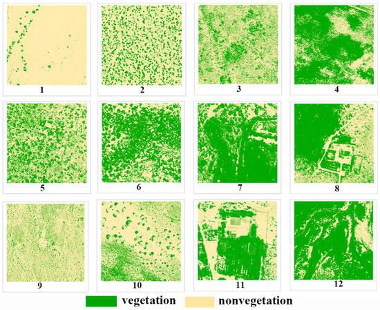
Figure 6. Thumbnails of 12 UAV image results extracted based on the LMM.

Table 6. Accuracy verification of LMM ^a.

No.	$\mathbf{a}$	$\mathbf{b}$	$\mathbf{c}$	$\mathbf{d}$	$\mathbf{A}\mathbf{c}\mathbf{c}\mathbf{u}\mathbf{r}\mathbf{a}\mathbf{c}\mathbf{y}$	$\mathbf{P}\mathbf{r}\mathbf{e}\mathbf{c}\mathbf{i}\mathbf{s}\mathbf{i}\mathbf{o}\mathbf{n}$	$\mathbf{R}\mathbf{e}\mathbf{c}\mathbf{a}\mathbf{l}\mathbf{l}$	$\mathbf{f}$	$\mathbf{O}\mathbf{A}$	$\mathbf{U}\mathbf{A}$
1	72	28	3	97	0.845	0.960	0.720	0.823	0.030	0.280
2	163	37	40	160	0.808	0.803	0.815	0.809	0.200	0.185
3	231	69	3	297	0.880	0.987	0.770	0.865	0.010	0.230
4	136	14	20	130	0.887	0.872	0.907	0.889	0.133	0.093
5	239	61	5	295	0.890	0.980	0.797	0.879	0.017	0.203
6	216	34	2	248	0.928	0.991	0.864	0.923	0.008	0.136
7	97	3	8	92	0.945	0.924	0.970	0.946	0.080	0.030
8	229	21	33	217	0.892	0.874	0.916	0.895	0.132	0.084
9	166	34	6	194	0.900	0.965	0.830	0.892	0.030	0.170
10	177	23	21	179	0.890	0.894	0.885	0.889	0.105	0.115
11	176	24	11	189	0.913	0.941	0.880	0.910	0.055	0.120
12	179	21	27	173	0.880	0.869	0.895	0.882	0.135	0.105

^a a, b, c, and d in the Table 6 header indicate extracted results and results made from the confusion matrix.

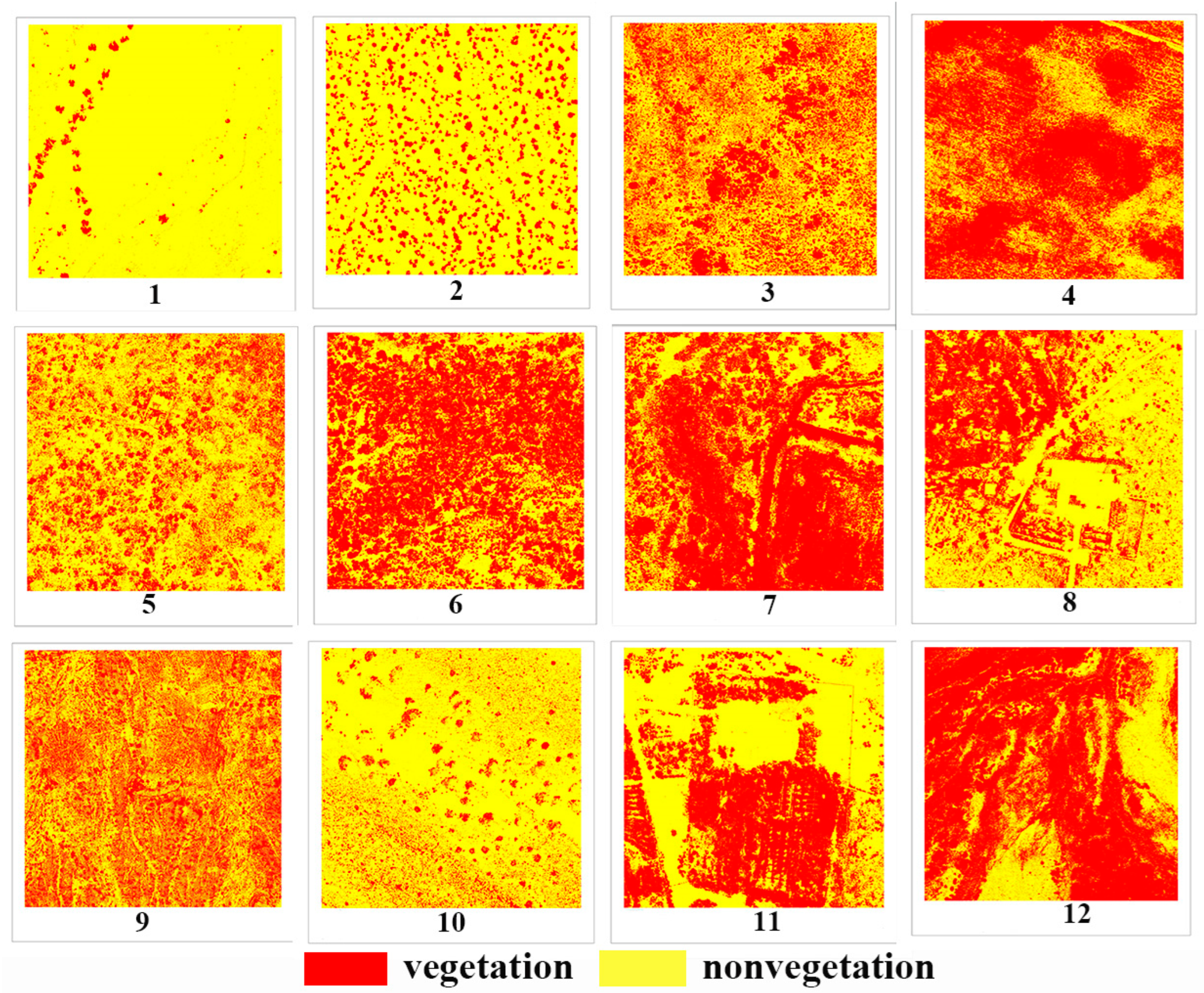
4.5. SVM

The SVM was used to extract FVC from the 12 images, and extraction outcome images were obtained (Figure 7; Table 7).

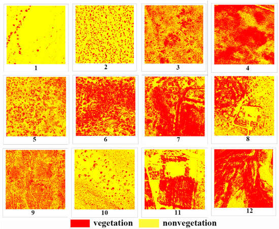
Figure 7. Thumbnail extraction of 12 UAV image results based on the SVM.

Table 7. Accuracy verification of SVM ^a.

No.	$\mathbf{a}$	$\mathbf{b}$	$\mathbf{c}$	$\mathbf{d}$	$\mathbf{A}\mathbf{c}\mathbf{c}\mathbf{u}\mathbf{r}\mathbf{a}\mathbf{c}\mathbf{y}$	$\mathbf{P}\mathbf{r}\mathbf{e}\mathbf{c}\mathbf{i}\mathbf{s}\mathbf{i}\mathbf{o}\mathbf{n}$	$\mathbf{R}\mathbf{e}\mathbf{c}\mathbf{a}\mathbf{l}\mathbf{l}$	$\mathbf{f}$	$\mathbf{O}\mathbf{A}$	$\mathbf{U}\mathbf{A}$
1	78	22	3	97	0.875	0.963	0.780	0.862	0.030	0.220
2	159	41	1	199	0.895	0.994	0.795	0.883	0.005	0.205
3	294	6	4	296	0.983	0.987	0.980	0.983	0.013	0.020
4	135	15	5	145	0.933	0.964	0.900	0.931	0.033	0.100
5	183	117	26	274	0.762	0.876	0.610	0.719	0.087	0.390
6	231	19	12	238	0.938	0.951	0.924	0.937	0.048	0.076
7	99	1	8	92	0.955	0.925	0.990	0.957	0.080	0.010
8	189	61	17	233	0.844	0.917	0.756	0.829	0.068	0.244
9	189	11	31	169	0.895	0.859	0.945	0.900	0.155	0.055
10	192	8	1	199	0.978	0.995	0.960	0.977	0.005	0.040
11	186	14	5	195	0.953	0.974	0.930	0.951	0.025	0.070
12	169	31	9	191	0.900	0.949	0.845	0.894	0.045	0.155

^a a, b, c, and d in the Table 7 header indicate extracted results and results made from the confusion matrix.

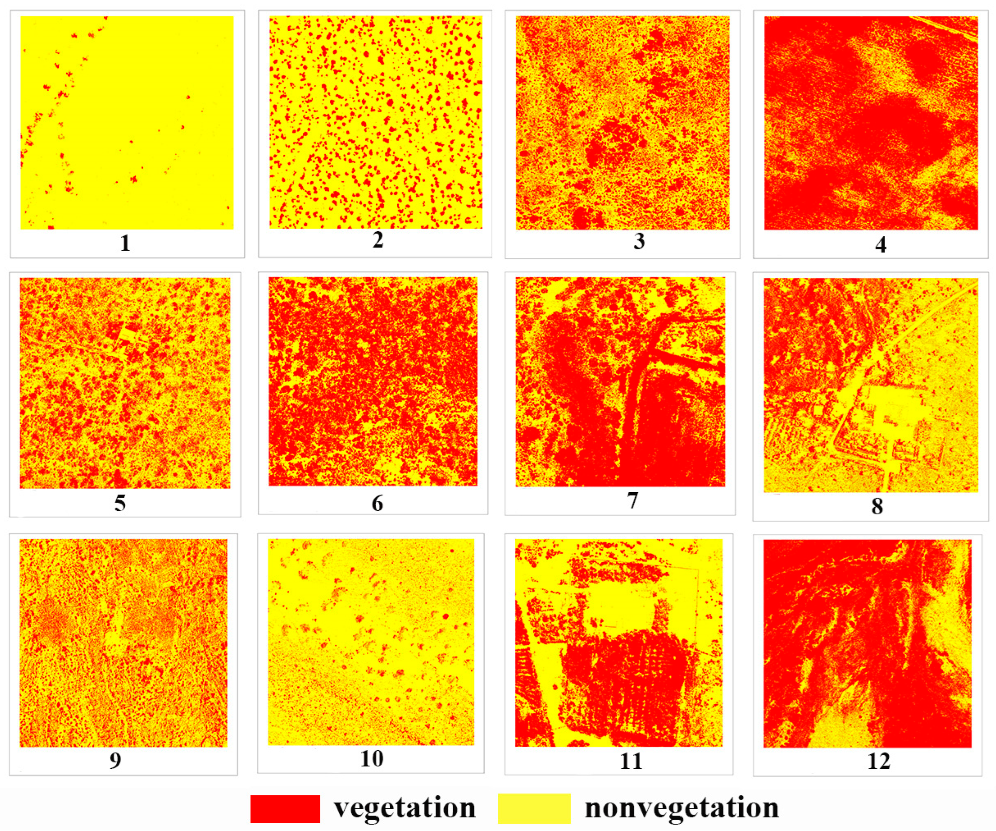
4.6. NN

The NN was used to extract FVC from the 12 images, and extraction outcome images were generated (Figure 8; Table 8).

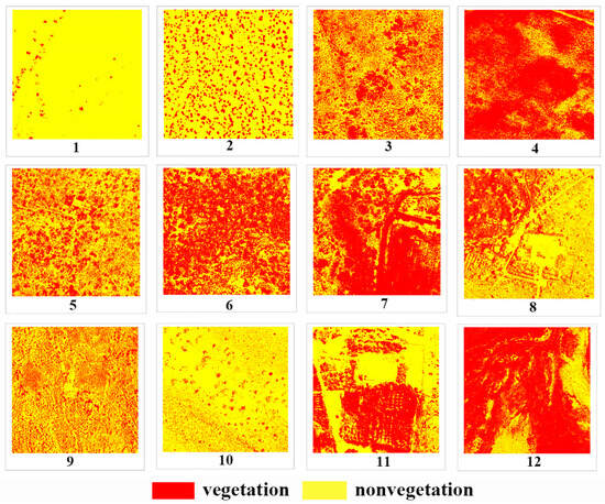
Figure 8. Thumbnail extraction of 12 UAV image results based on the NN.

Table 8. Accuracy verification of NN ^a.

No.	$\mathbf{a}$	$\mathbf{b}$	$\mathbf{c}$	$\mathbf{d}$	$\mathbf{A}\mathbf{c}\mathbf{c}\mathbf{u}\mathbf{r}\mathbf{a}\mathbf{c}\mathbf{y}$	$\mathbf{P}\mathbf{r}\mathbf{e}\mathbf{c}\mathbf{i}\mathbf{s}\mathbf{i}\mathbf{o}\mathbf{n}$	$\mathbf{R}\mathbf{e}\mathbf{c}\mathbf{a}\mathbf{l}\mathbf{l}$	$\mathbf{f}$	$\mathbf{O}\mathbf{A}$	$\mathbf{U}\mathbf{A}$
1	49	51	0	100	0.745	1.000	0.490	0.658	0.000	0.510
2	163	37	2	198	0.903	0.988	0.815	0.893	0.010	0.185
3	296	4	4	296	0.987	0.987	0.987	0.987	0.013	0.013
4	138	162	168	132	0.450	0.451	0.460	0.455	0.560	0.540
5	214	86	2	298	0.853	0.991	0.713	0.829	0.007	0.287
6	214	36	38	212	0.852	0.849	0.856	0.853	0.152	0.144
7	97	3	8	92	0.945	0.924	0.970	0.946	0.080	0.030
8	174	76	48	202	0.752	0.784	0.696	0.737	0.192	0.304
9	190	10	6	194	0.960	0.969	0.950	0.960	0.030	0.050
10	172	28	0	200	0.930	1.000	0.860	0.925	0.000	0.140
11	176	24	13	187	0.908	0.931	0.880	0.905	0.065	0.120
12	182	18	46	154	0.840	0.798	0.910	0.850	0.230	0.090

^a a, b, c, and d in the Table 8 header indicate extracted results and results made from the confusion matrix.

4.7. Confusion Matrix

(1)

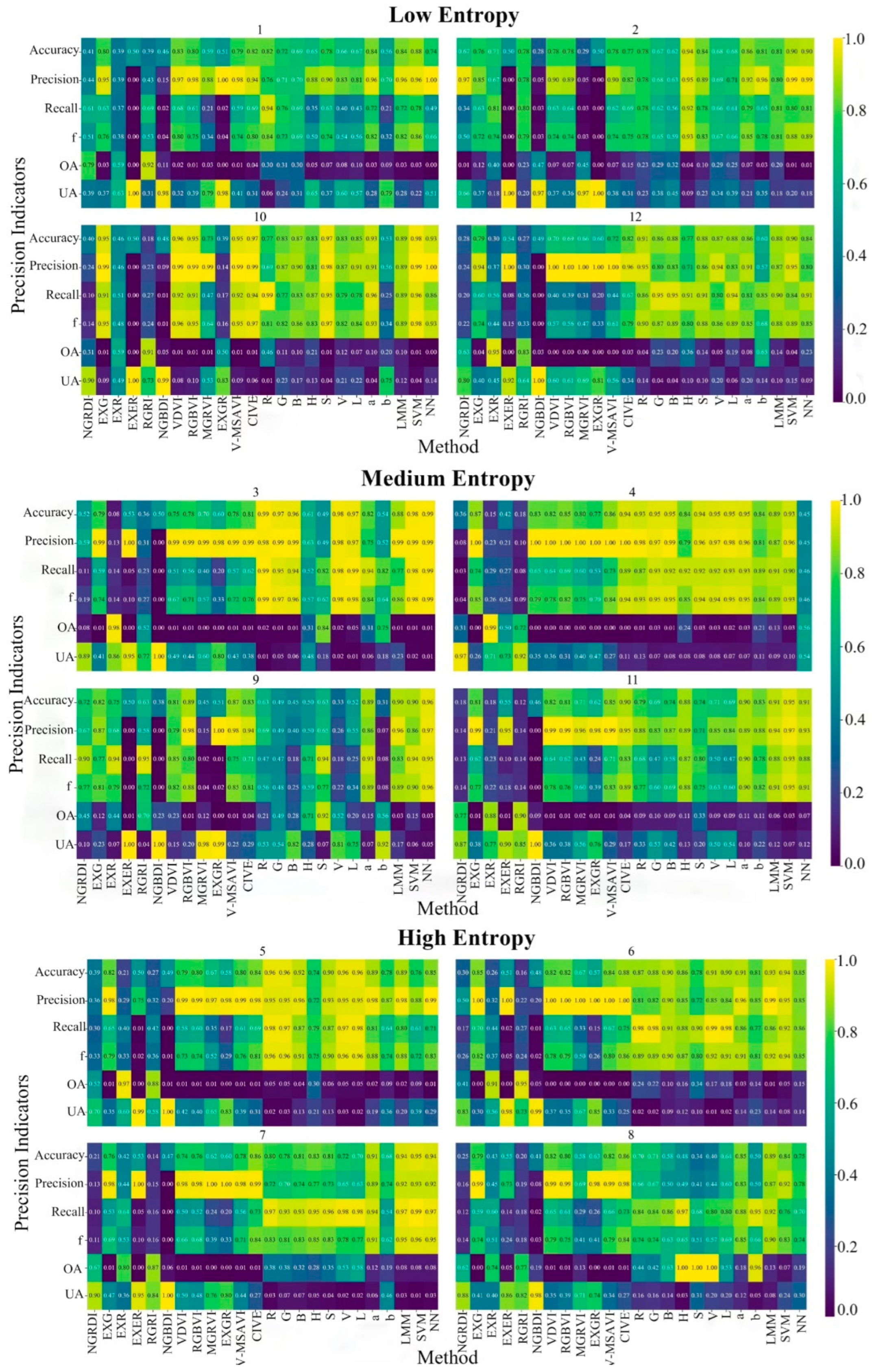
Otsu–VVIs

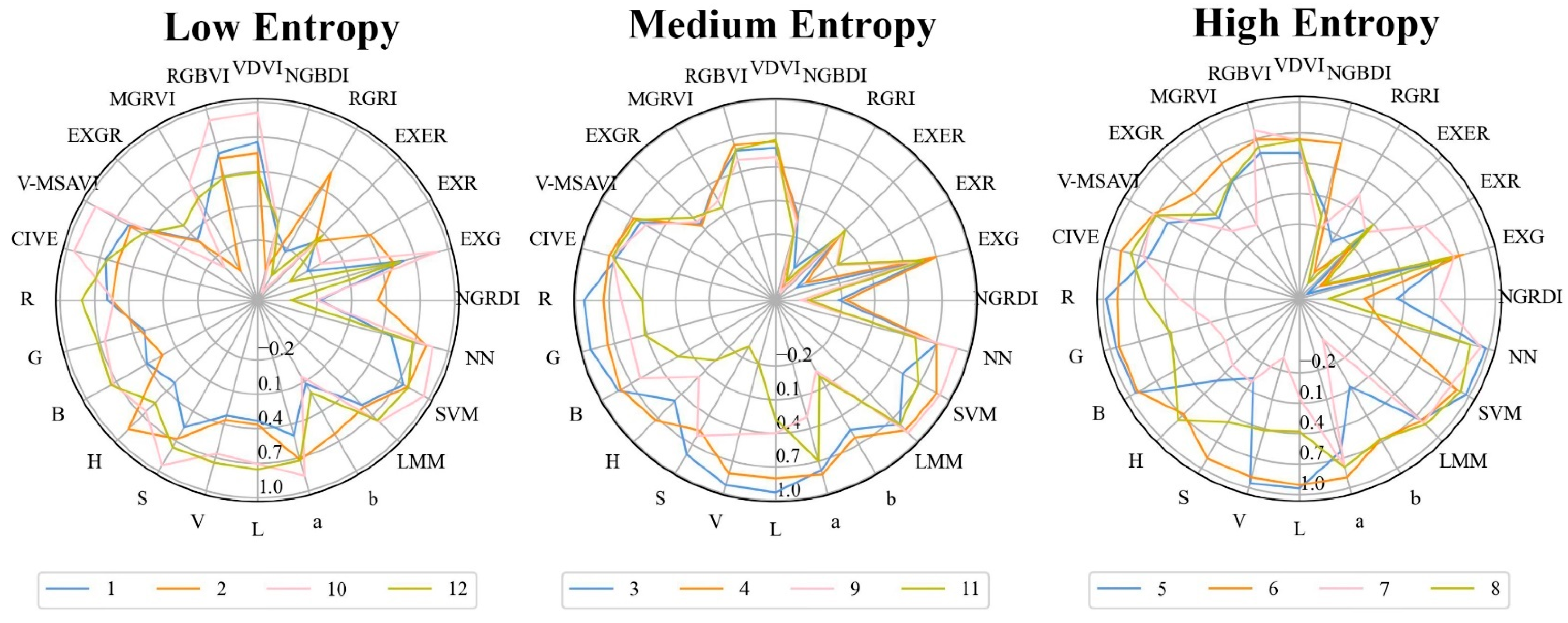
The vegetation indices EXG, VDVI, RGBVI, V-MSAVI, and CIVE display universality and stability across various entropy conditions (Figure 9). For the low-entropy images, these indices demonstrate an $Accuracy$ range of 0.7–0.96, indicating excellent differentiation between vegetation and nonvegetation. $Precision$ ranges from 0.85 to 1, showing high vegetation recognition precision. Although $Recall$ is generally good, some misclassification occurs. For the medium-entropy images, $Accuracy$ slightly drops to 0.75–0.94, but $Precision$ increases to 0.87–1. $Recall$ is similar to that for the low-entropy images (prone to misclassification). For the high-entropy images, $Accuracy$ ranges from 0.74 to 0.86 and $Precision$ is 0.98–1; however, the vegetation extraction accuracy is notably lower than that for the low- and medium-entropy images. $Recall$ is still generally good but includes some misclassifications.

Figure 9. Thumbnails of heat maps of high, medium, and low entropy values.

(2)

Color Space Method

Each color component (R, G, B, H, S, V, L, a, and b) exhibits distinct stability and universality between entropy conditions (Figure 9). For the low-entropy images, $Accuracy$ is 0.53–0.97 and $Precision$ is 0.56–1, indicating good overall model performance and high vegetation extraction precision, respectively. For the medium-entropy images, $Accuracy$ is 0.31–0.94 and $Precision$ is 0.07–0.98, showing notable declines in overall performance and vegetation extraction precision, respectively, compared with those for the low-entropy images. For the high-entropy images, $Accuracy$ ranges from 0.34 to 0.96 and $Precision$ from 0.41 to 0.98, suggesting lower overall performance and precision in vegetation extraction, respectively, than for the low- and medium-entropy images. Furthermore, more misclassifications are observed here than for the low- and medium-entropy images.

(3)

LMM

For the low-, medium-, and high-entropy images, the model’s overall performance, vegetation extraction precision, and accuracy significantly improve (Figure 9). Specifically, for the low-entropy images, $Accuracy$ is between 0.79 and 0.89, $Precision$ is 0.87–0.97, and $Recall$ is between 0.59 and 0.9, with few misclassifications. As for the medium-entropy images, $Accuracy$ is between 0.88 and 0.91, $Precision$ is between 0.87 and 0.99, and $Recall$ is 0.77–0.91, with few misclassifications. For the high-entropy images, $Accuracy$ is 0.89–0.94, $Precision$ is 0.87–0.99, and $Recall$ is 0.80–0.97, with few misclassifications. Overall, the overall model performance and vegetation extraction accuracy and precision are notably better than those under the Otsu–VVI and color space methods.

(4)

SVM

For the low-entropy images, FVC extraction $Accuracy$ is 0.89–0.94, $Precision$ is 0.87–0.99, and $Recall$ is 0.78–0.96, with few misclassifications (Figure 9). For the medium-entropy images, $Accuracy$ ranges from 0.89 to 0.98, $Precision$ from 0.86 to 0.99, and $Recall$ from 0.86 to 0.98, with few misclassifications. For the high-entropy images, $Accuracy$ is 0.76–0.95, $Precision$ is 0.88–0.95, and $Recall$ is 0.61–0.99, with few misclassifications. These indicate high stability and precision across all entropy conditions.

(5)

NN

For the low-entropy images, $Accuracy$ ranges from 0.74 to 0.93, $Precision$ from 0.8 to 1, and $Recall$ from 0.49 to 0.91, with few misclassifications (Figure 9). These suggest good overall model performance and significantly good vegetation extraction precision. For the medium-entropy images, $Accuracy$ is 0.45–0.99, $Precision$ is 0.45–0.99, and $Recall$ is 0.46–0.99, with few misclassifications. These show good overall model performance and vegetation extraction precision.

4.8. Kappa Coefficient

(1)

Otsu–VVIs

For images with low, medium, and high entropy values, the VVIs EXG, VDVI, RGBVI, V-MSAVI, and CIVE show optimal vegetation extraction accuracy. In particular, the CIVE demonstrates high precision across all entropy conditions, with kappa coefficients ranging from 0.54 to 0.94 (Figure 10; Table 9).

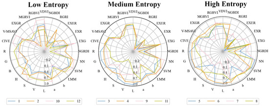
Figure 10. Thumbnails of radars of high, medium, and low entropy values.

Table 9. Kappa of FVC extraction using Otsu–VVIs.

No.	VVIs	Kappa
1	NGRDI	−0.180
	EXG	0.600
	EXR	−0.220
	EXER	0.000
	RGRI	−0.230
	NGBDI	−0.090
	VDVI	0.660
	RGBVI	0.600
	MGRVI	0.180
	EXGR	0.020
	V-MSAVI	0.580
	CIVE	0.650
2	NGRDI	0.330
	EXG	0.515
	EXR	0.420
	EXER	0.000
	RGRI	0.565
	NGBDI	−0.445
	VDVI	0.560
	RGBVI	0.560
	MGRVI	−0.425
	EXGR	0.000
	V-MSAVI	0.555
	CIVE	0.540
3	NGRDI	0.033
	EXG	0.583
	EXR	−0.840
	EXER	0.050
	RGRI	−0.287
	NGBDI	0.000
	VDVI	0.503
	RGBVI	0.553
	MGRVI	0.400
	EXGR	0.193
	V-MSAVI	0.563
	CIVE	0.613
4	NGRDI	−0.287
	EXG	0.740
	EXR	−0.693
	EXER	−0.212
	RGRI	−0.640
	NGBDI	0.653
	VDVI	0.640
	RGBVI	0.693
	MGRVI	0.600
	EXGR	0.533
	V-MSAVI	0.727
	CIVE	0.887
5	NGRDI	−0.227
	EXG	0.643
	EXR	−0.575
	EXER	0.007
	RGRI	−0.460
	NGBDI	−0.010
	VDVI	0.570
	RGBVI	0.590
	MGRVI	0.340
	EXGR	0.167
	V-MSAVI	0.603
	CIVE	0.680
6	NGRDI	−0.163
	EXG	0.700
	EXR	−0.476
	EXER	0.024
	RGRI	−0.684
	NGBDI	−0.036
	VDVI	0.632
	RGBVI	0.648
	MGRVI	0.332
	EXGR	0.148
	V-MSAVI	0.672
	CIVE	0.752
7	NGRDI	−0.570
	EXG	0.520
	EXR	−0.160
	EXER	0.050
	RGRI	−0.710
	NGBDI	−0.060
	VDVI	0.490
	RGBVI	0.510
	MGRVI	0.240
	EXGR	0.200
	V-MSAVI	0.550
	CIVE	0.720
8	NGRDI	−0.500
	EXG	0.584
	EXR	−0.148
	EXER	0.092
	RGRI	−0.596
	NGBDI	−0.172
	VDVI	0.644
	RGBVI	0.600
	MGRVI	0.164
	EXGR	0.252
	V-MSAVI	0.648
	CIVE	0.720
9	NGRDI	0.450
	EXG	0.650
	EXR	0.495
	EXER	−0.005
	RGRI	0.255
	NGBDI	−0.235
	VDVI	0.625
	RGBVI	0.785
	MGRVI	−0.095
	EXGR	0.010
	V-MSAVI	0.735
	CIVE	0.665
10	NGRDI	−0.210
	EXG	0.905
	EXR	−0.085
	EXER	0.000
	RGRI	−0.640
	NGBDI	−0.045
	VDVI	0.915
	RGBVI	0.900
	MGRVI	0.465
	EXGR	−0.317
	V-MSAVI	0.910
	CIVE	0.935
11	NGRDI	−0.640
	EXG	0.620
	EXR	−0.640
	EXER	0.095
	RGRI	−0.755
	NGBDI	−0.090
	VDVI	0.635
	RGBVI	0.615
	MGRVI	0.415
	EXGR	0.240
	V-MSAVI	0.705
	CIVE	0.790
12	NGRDI	−0.430
	EXG	0.570
	EXR	−0.395
	EXER	0.080
	RGRI	−0.470
	NGBDI	−0.025
	VDVI	0.395
	RGBVI	0.390
	MGRVI	0.310
	EXGR	0.195
	V-MSAVI	0.440
	CIVE	0.635

(2)

Color Space Method

The ‘a’ component achieves high accuracy in images with low, medium, and high entropy values, with kappa coefficients ranging from 0.63 to 0.89. This indicates that this component has significant discriminative ability in extracting vegetation cover across various entropy conditions (Table 10).

Table 10. Kappa of FVC extraction using color space method.

No.	Components	Kappa
1	R	0.640
	G	0.450
	B	0.390
	H	0.300
	S	0.560
	V	0.320
	L	0.330
	a	0.690
	b	0.120
2	R	0.550
	G	0.330
	B	0.235
	H	0.870
	S	0.675
	V	0.360
	L	0.365
	a	0.720
	b	0.625
3	R	0.973
	G	0.940
	B	0.930
	H	0.213
	S	−0.023
	V	0.953
	L	0.941
	a	0.633
	b	0.070
4	R	0.860
	G	0.907
	B	0.907
	H	0.680
	S	0.887
	V	0.893
	L	0.907
	a	0.893
	b	0.673
5	R	0.923
	G	0.923
	B	0.830
	H	0.483
	S	0.803
	V	0.923
	L	0.930
	a	0.787
	b	0.550
6	R	0.748
	G	0.764
	B	0.808
	H	0.728
	S	0.560
	V	0.816
	L	0.804
	a	0.824
	b	0.628
7	R	0.590
	G	0.550
	B	0.610
	H	0.670
	S	0.610
	V	0.450
	L	0.400
	a	0.820
	b	0.350
8	R	0.404
	G	0.420
	B	0.213
	H	−0.032
	S	−0.312
	V	−0.204
	L	0.272
	a	0.700
	b	−0.004
9	R	0.255
	G	−0.025
	B	−0.095
	H	0.000
	S	0.021
	V	−0.335
	L	0.045
	a	0.775
	b	−0.468
10	R	0.535
	G	0.655
	B	0.735
	H	0.653
	S	0.940
	V	0.665
	L	0.705
	a	0.865
	b	0.050
11	R	0.585
	G	0.380
	B	0.490
	H	0.760
	S	0.475
	V	0.415
	L	0.380
	a	0.790
	b	0.670
12	R	0.815
	G	0.720
	B	0.755
	H	0.545
	S	0.760
	V	0.745
	L	0.755
	a	0.725
	b	0.210

(3)

LMM

This model shows higher vegetation extraction accuracy in the low-entropy images, with kappa coefficients between 0.62 and 0.78. For the medium-entropy images, the kappa coefficients range from 0.76 to 0.89, indicating an improvement in vegetation extraction accuracy compared with that for the low-entropy images. In the high-entropy images, the kappa coefficients range from 0.78 to 0.89, suggesting that the model’s overall precision in vegetation extraction is higher than that for the low-entropy images but lower than that for the medium-entropy images (Table 11).

Table 11. Kappa of FVC extraction using LMM.

No.	Kappa
1	0.690
2	0.615
3	0.760
4	0.773
5	0.780
6	0.856
7	0.890
8	0.784
9	0.800
10	0.780
11	0.825
12	0.760

(4)

SVM

In FVC extraction using the SVM, the low-entropy images show kappa coefficients ranging from 0.75 to 0.96, indicating high vegetation extraction accuracy. The medium-entropy images have kappa coefficients ranging from 0.79 to 0.97, showing a slight decline in accuracy compared with the low-entropy images, but the overall performance of the model remains good. The high-entropy images have kappa coefficients of 0.52 and 0.91, indicating a decrease in vegetation extraction accuracy compared with that for the low- and medium-entropy images (Table 12).

Table 12. Kappa of FVC extraction using SVM.

No.	Kappa
1	0.750
2	0.790
3	0.967
4	0.867
5	0.523
6	0.876
7	0.910
8	0.688
9	0.790
10	0.955
11	0.905
12	0.800

(5)

NN

Except the first low-entropy image, which has a kappa coefficient of 0.49, all low-entropy images have kappa coefficients of 0.68–0.86, indicating low precision in sparse vegetation areas. Except the fourth medium-entropy image, which has a kappa of −0.1, the medium-entropy images have kappa coefficients ranging from 0.82 to 0.97, showing high precision in extracting widely distributed vegetation but lower precision in extracting sporadically distributed vegetation. Except the eighth high-entropy image, which has a kappa coefficient of 0.50, the high-entropy images have kappa coefficients of 0.70 to 0.89, indicating lower precision in extracting vegetation in areas with sparse herbaceous vegetation and widespread soil backgrounds (Table 13).

Table 13. Kappa of FVC extraction using NN.

No.	Kappa
1	0.490
2	0.805
3	0.973
4	−0.100
5	0.707
6	0.704
7	0.890
8	0.504
9	0.920
10	0.860
11	0.815
12	0.680

5. Discussion

5.1. Comparison of Differentiated Scenarios and Entropy for FVC Extraction

(1)

Sparse Shrub Areas with Similar Backgrounds (No. 1 and No. 2)

Both are low-entropy images. In No. 1, the sparse yellow vegetation blends visually with its soil background in color and texture. This reduces the applicability of extraction methods other than the vegetation indices EXG, VDVI, RGBVI, V-MSAVI, and CIVE and the ‘b’ component of the color space method. These methods have limitations in distinguishing subtle differences, affecting the accuracy and reliability of the overall data analysis. Conversely, No. 2 displays a clearer contrast between vegetation and the background, improving the applicability and effectiveness of up to 20 high-precision FVC extraction methods (including the above). This highlights the importance of environmental background differences for the selection of vegetation extraction methods and data interpretation. Xie et al. (2020) introduced a new red–green–blue ratio vegetation index, which showed 93.5% accuracy in vegetation cover extraction using simple RGB data [39]. However, this is clearly not suitable for FVC extraction in arid and semiarid regions.

(2)

Mixed Grass–Shrub Areas with Distinct Ground Vegetation Demarcation (No. 3 and No. 10)

Both images cover mixed grass–shrub areas but show significant differences in the distinctiveness of surface vegetation, so the same high-precision FVC extraction methods apply to both images except the ‘S’ component. Specifically, the content of No. 10, a low-entropy image, is uniform and simple, where the ‘S’ component (saturation) demonstrates high accuracy in vegetation extraction. Therefore, in environments with simple, sparse vegetation distributions, the ‘S’ component can effectively distinguish between vegetated and nonvegetated areas, thus enhancing extraction accuracy. No. 3, a medium-entropy image, is visually more complex and diverse, containing more information and noise due to its mix of vegetation and nonvegetation and different surface features, reducing the performance of the ‘S’ component in vegetation extraction. This complexity sharply differs from the simpler, sparser vegetation distribution in No. 10, further highlighting how environmental complexity affects the choice and effectiveness of UAV data analysis methods, as noted by Mariana et al. (2017) [40].

(3)

Areas Cooccupied by Shrubs and Sparse Herbaceous Vegetation (No. 4 and No. 12)

In these scenarios, the same methods apply to both images except NNs, which show differing efficiencies. No. 4, a medium-entropy image, has a complex distribution of shrubs and grass, including unevenly distributed, densely interwoven vegetation structures, and variable surface features, which increase classification difficulty, compromising the performance of the NN model. Similar to the findings by Yan et al. (2019), environmental complexity significantly hinders NN performance [41]. By contrast, No. 12, a low-entropy image, may have simpler or more regular vegetation and terrain distribution despite also having shrubs and sparse grass, providing a more manageable data structure for the NN. Additionally, No. 12 may benefit from optimized lighting conditions, further enhancing data processing efficiency and accuracy. Thus, environmental complexity significantly affects the effectiveness of NN methods in vegetation classification.

(4)

Extensive Shrub Areas with Minor Grassland Integration (No. 6 and No. 7)

Both are medium-entropy images. Up to 19 methods are suitable for these widely, uniformly vegetated areas, mainly because the adequate resolution and spectral information of the images allow these high-precision methods to better process and analyze the characteristics of extensive, uniform vegetation distributions. Zhang et al. (2022) demonstrated that random forest models perform particularly well in processing such uniform vegetation distributions in arid regions [42]. Additionally, these methods benefit from their algorithms’ high data processing capability and robustness to environmental noise and background variations, which are crucial for extensively vegetated areas. Therefore, methods besides the five vegetation indices (NGRDI, EXR, EXER, RGRI, NGBDI) enable a more comprehensive assessment and accurate extraction of vegetation cover in such environments.

(5)

Mixed Grass–Shrub Areas with Indistinguishable Soil Backgrounds (No. 9)

In this medium-entropy image, the spectral properties of the soil closely resemble those of the surrounding vegetation, so traditional vegetation indices cannot effectively distinguish between vegetation and soil. This significantly reduces the number of suitable high-precision vegetation extraction methods, especially in the color space method, where only the R, S, and ‘a’ component exhibit high extraction precision. Adjusting the UAV’s shooting angle and optimizing lighting conditions, as suggested by Catherine et al. (2013), can help improve vegetation extraction in such complex scenarios [43]. Data quality should be optimized through adjustments in image capture timing, lighting conditions, and camera angles to improve vegetation extraction in complex scenarios. Flying under optimal sunlight conditions, such as early morning or late evening, can avoid the high reflectance and intense shadows caused by direct midday sunlight and reduce spectral differences between vegetation and soil due to changes in solar angle. Adjusting the UAV’s shooting angle can capture more dimensional surface information, increasing the visual and spectral distinction between vegetation and soil in images. This improves the recognition and classification accuracy of vegetation features in UAV images and optimizes vegetation cover estimates in areas with complex soil backgrounds.

(6)

Complex Vegetation Types with High Cover and Architectural Interference (No. 5, 8, and 11)

No. 5 and No. 8 are high-entropy images, whereas Image 11 is a medium-entropy one. In this scenario, the same high-precision vegetation extraction methods are applied to No. 5 and No. 11 due to their similar settings. As for No. 8, only 13 FVC extraction methods are available, fewer than those for the two other images. Specifically, only five components (G, B, H, S, V, and b) in the color space method are suitable. This is mainly because of the extensive presence of sparse herbaceous vegetation and the soil background in Image 8, which lowers the accuracy of these color space components in distinguishing between vegetation and nonvegetation. Li et al. (2019) have similarly highlighted the limitations of vegetation indices in complex, mixed environments [44].

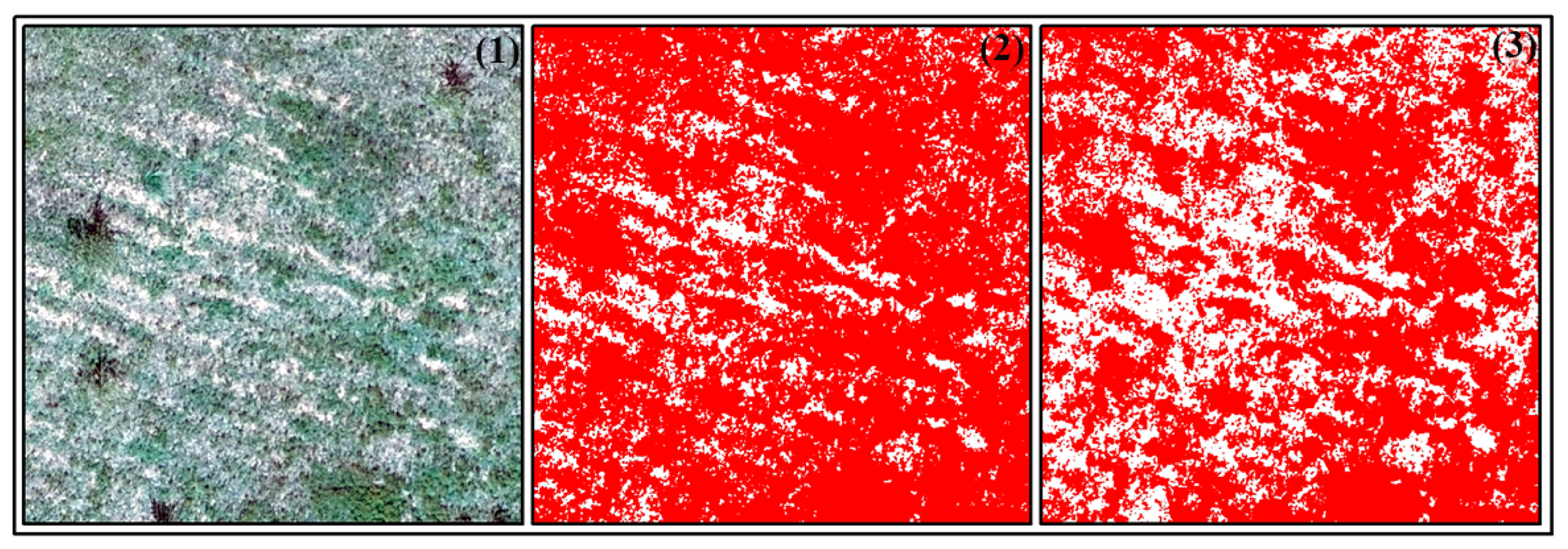
In conclusion, the effectiveness of vegetation cover extraction in different entropy scenarios significantly depends on the entropy level and scene complexity, so selecting extraction methods suitable for specific backgrounds and conditions is crucial. Future research should further explore how to integrate the advantages of various methods—traditional vegetation indices, machine learning techniques, and recent image processing algorithms—to adapt to diverse environmental scenarios and improve vegetation extraction precision (Figure 11).

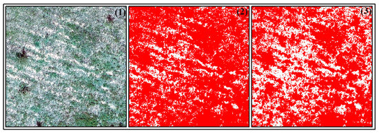
Figure 11. (1)–(3) Original image, SVM and NN. Red: FVC; white: non-FVC.

5.2. Comparison of FVC Extraction Methods

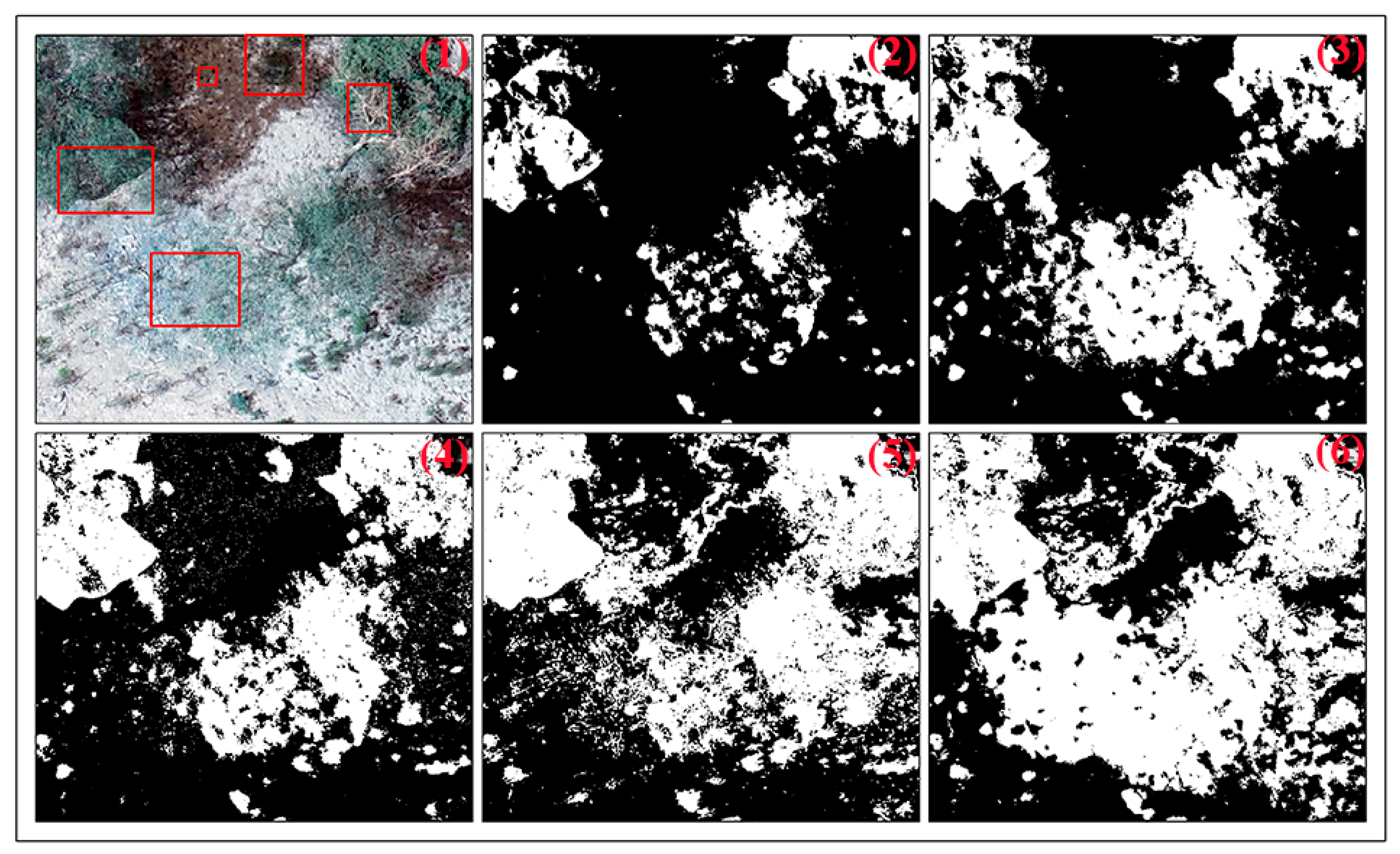
This study uses UAV image data and 24 FVC extraction methods to explore vegetation cover extraction in typical arid areas in Xinjiang across different entropy values. These methods encompass widely used vegetation indices, the color space method, LMM, and machine learning algorithms (SVM and NN) that are becoming mainstream in various research domains. Under different entropy conditions, the optimal FVC extraction methods are the CIVE, the ‘a’ component of the color space method, LMM, and machine learning. However, each method has distinct strengths and limitations in extracting FVC under specific conditions, such as shadows, vegetation under shadows, yellow vegetation, sparse vegetation, and biological soil crusts. These are detailed as follows (Figure 12, 15 m × 14 m):

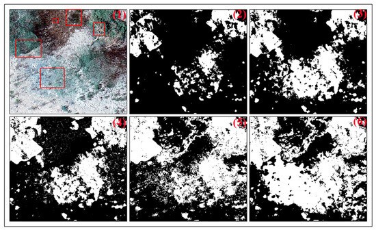
Figure 12. (1) Original, (2) CIVE, (3) ‘a’ component, (4) LMM, (5) SVM, (6) NN. White: FVC; black: non-FVC. The red squares in subplot a highlight the particular vegetation encountered during the extraction process and its particular environment.

(1)

CIVE

The CIVE performs well in distinguishing pure shadows from vegetation but identifies biological soil crusts, sparse vegetation, yellow vegetation, and their branches as nonvegetation, which aligns with findings in desert regions by Hao et al. (2020), in which areas under shadows are also frequently misclassified, highlighting the need for strict control over lighting and angles during UAV image capture to enhance FVC extraction accuracy under these conditions [45]. Vegetation under shadows is also frequently misclassified. This necessitates strict control over lighting and angles during UAV image capture to enhance FVC extraction accuracy under these conditions.

(2)

Color Space Method

The ‘a’ component improves extraction accuracy for sparse vegetation and pure shadow parts but identifies biological soil crusts, vegetation under shadows, yellow vegetation, and branch areas as nonvegetation, consistent with previous research on urban vegetation cover mapping [46]. Threshold adjustment can optimize the distinction between vegetation and nonvegetation for optimal accuracy.

(3)

LMM

Compared with the CIVE and the ‘a’ component, the LMM significantly improves extraction accuracy for pure shadows, sparse vegetation, vegetation under shadows, and biological soil crusts, but it has limitations with yellow vegetation and branches. Its overall accuracy is significantly higher than that of the CIVE and the ‘a’ component, as reported by Ni (2023) [46].

(4)

Machine Learning Algorithms

The SVM and NN outperform the other methods in extracting yellow vegetation and its branches. However, they have limitations in extracting pure shadow and sparse vegetation parts, with the NN performing notably worse. Vegetation under shadows and biological soil crusts are also not effectively recognized, with the SVM generally outperforming the NN. Moreover, despite these methods’ high extraction accuracy for pure green vegetation, limitations remain in extracting biological soil crusts, yellow vegetation, branches, shadows, and vegetation under shadows. Future research should explore combining these methods’ strengths to develop more accurate and practical strategies, particularly for vegetation cover extraction in arid and semiarid areas [47].

5.3. Accuracy of UAV Remote Sensing Images

UAV remote sensing bridges the gap between ground measurements and low-spatial-resolution satellite sensing, providing fine centimeter-level ground data without the constraints of timing or other factors [48]. This particularly holds in specific small-scale monitoring tasks, where UAV operation costs are significantly lower than those of traditional satellite sensing methods. In practical applications, high-resolution UAV imagery captures more details, greatly enhancing the accuracy of assessments of vegetation type, health, and cover. The high-resolution UAV imagery is one of its greatest advantages, allowing researchers to observe and analyze surface features meticulously. However, whether the accuracy of vegetation cover extraction linearly increases with the resolution of the original images or the effect of resolution on FVC extraction stops being significant beyond a certain threshold remains a critical question. This issue should be discussed to optimize UAV remote sensing applications in ecological monitoring and environmental management. Current research indicates that although high-resolution imagery provides rich surface information, it can also introduce noise, especially in areas with unclear vegetation boundaries or dense vegetation, potentially decreasing FVC extraction accuracy [49]. Moreover, a high image resolution typically entails considerable data processing demands, requiring more advanced data processing hardware and high processing time and costs. Therefore, determining the optimal image resolution to balance accuracy and cost is an important direction for future research. Experimental and theoretical analyses should be performed to assess FVC extraction performance systematically at different resolutions and establish precise vegetation monitoring models. Finally, the lack of near-infrared (NIR) as well as multispectral data in this study greatly limits the ability to capture nuances in vegetation health, especially in the later stages of growth. Without the use of NIR or multispectral imagery, more detailed information on plant health and soil-vegetation interactions cannot be obtained. NIR data, however, are able to distinguish between healthy and stressed vegetation and are widely used in vegetation studies.

6. Conclusions

This study utilizes UAV data combined with Otsu–VVIs (EXG, EXR, EXER, NGRDI, NGBDI, RGRI, CIVE, V-MSAVI, EXGR, MGRVI, RGBVI, and VDVI), the color space method (R, G, B, H, S, V, L, a, and b), LMM, and two machine learning algorithms (SVM and NN) to extract fractional vegetation cover in different entropy scenarios in the arid regions of Xinjiang. The most effective methods for extracting fractional vegetation cover against the backdrop of the strong reflective soil found in arid and semiarid regions were identified and validated: the CIVE, the ‘a’ component in the color space method, LMM, and SVM.

Regarding the Otsu–VVIs in high-, medium-, and low-entropy images, the CIVE outperforms the other vegetation indices, with $Accuracy$ = 0.77–0.97 and $Precision$ = 0.82–1. These results highlight the CIVE’s superior overall performance, accuracy, and precision in vegetation extraction, with low rates of missed and false detections.

Regarding the color space method in high-, medium-, and low-entropy images, the ‘a’ component demonstrates superior FVC extraction accuracy compared with the other color components. It shows $Accuracy$ = 0.82–0.95 and $Precision$ = 0.75–0.96. These results emphasize the applicability of the ‘a’ component in extracting vegetation cover in the arid regions of Xinjiang.

The LMM achieves the following metrics in FVC extraction across high-, medium-, and low-entropy images: $Accuracy$ = 0.81–0.94, $Precision$ = 0.87–0.99. Therefore, the LMM provides high precision and accuracy in extracting vegetation cover in Xinjiang’s arid regions, with low rates of missed and false detections.

The SVM achieves the following values in FVC extraction across high-, medium-, and low-entropy images: $Accuracy$ = 0.76–0.98, $Precision$ = 0.88–0.95. Hence, the SVM is highly applicable for extracting FVC under different entropy conditions in Xinjiang’s arid and semiarid regions. On the contrary, the NN shows relatively lower accuracy in extracting vegetation cover under varying entropy conditions among sparse distributions of shrubs and grasslands in arid regions.

References

- Liu, C.; Zhang, X.; Wang, T.; Chen, G.; Zhu, K.; Wang, Q.; Wang, J. Detection of vegetation cover-age changes in the Yellow River Basin from 2003 to 2020. Ecol. Indic. 2022, 138, 108818. (In English) [Google Scholar] [CrossRef]
- Song, J.M.; Xia, N.; Hai, W.Y.; Tang, M.Y. Spatial-temporal variation of vegetation in Gobi region of Xinjiang based on NDVI-DFI model. Southwest China J. Agric. Sci. 2022, 35, 2867–2875. [Google Scholar]
- Zhao, J.; Li, J.; Zhang, Z.X.; Wu, S.L.; Zhong, B.; Liu, Q.H. A dataset of 16 m/10-day fractional vegetation cover of MuSyQ GF-series (2018–2020, China, Version 01). China Sci. Data 2022, 7, 221–230. [Google Scholar] [CrossRef]
- Zhang, S.; Yang, R.; Wenxing, H.; Wang, L.; Shuang, L.; Song, H.; Zhao, W.; Li, L. Analysis of Fractional Vegetation Cover Changes and Driving Forces on Both Banks of Yongding River Before and After Ecological Water Replenishment. Ecol. Environ. Sci. 2023, 32, 264–273. [Google Scholar]
- Chen, X.; Lv, X.; Ma, L.; Chen, A.; Zhang, Q.; Zhang, Z. Optimization and Validation of Hyperspectral Estimation Capability of Cotton Leaf Nitrogen Based on SPA and RF. Remote Sens. 2022, 14, 5201. [Google Scholar] [CrossRef]
- Li, Y.; Sun, J.; Wang, M.; Guo, J.; Wei, X.; Shukla, M.K.; Qi, Y. Spatiotemporal Variation of Fractional Vegetation Cover and Its Response to Climate Change and Topography Characteristics in Shaanxi Province, China. Appl. Sci. 2023, 13, 11532. [Google Scholar] [CrossRef]
- Cai, Y.; Zhang, M.; Lin, H. Estimating the Urban Fractional Vegetation Cover Using an Object-Based Mixture Analysis Method and Sentinel-2 MSI Imagery. IEEE J. Sel. Top. Appl. Earth Obs. Remote Sens. 2020, 13, 341–350. [Google Scholar] [CrossRef]
- Liang, J.; Liu, D. Automated estimation of daily surface water fraction from MODIS and Landsat images using Gaussian process regression. Int. J. Remote Sens. 2021, 42, 4261–4283. [Google Scholar] [CrossRef]
- Jia, X.; Shao, M.; Zhu, Y.; Luo, Y. Soil moisture decline due to afforestation across the Loess Plateau, China. J. Hydrol. 2017, 546, 113–122. [Google Scholar] [CrossRef]
- Elmendorf, S.C.; Henry, G.H.; Hollister, R.D.; Björk, R.G.; Bjorkman, A.D.; Callaghan, T.V.; Collier, L.S.; Cooper, E.J.; Cornelissen, H.C.; Day, T.A.; et al. Global assessment of experimental climate warming on tundra vegetation: Heterogeneity over space and time. Ecol. Lett. 2012, 15, 164–175. [Google Scholar] [CrossRef]
- Wang, N.; Guo, Y.; Wei, X.; Zhou, M.; Wang, H.; Bai, Y. UAV-based remote sensing using visible and multi-spectral indices for the estimation of vegetation cover in an oasis of a desert. Ecol. Indic. 2022, 141, 109155. [Google Scholar] [CrossRef]
- Zhong, G.; Chen, J.; Huang, R.; Yi, S.; Qin, Y.; You, H.; Han, X.; Zhou, G. High Spatial Resolution Fractional Vegetation Coverage Inversion Based on UAV and Sentinel-2 Data: A Case Study of Alpine Grassland. Remote Sens. 2023, 15, 4266. [Google Scholar] [CrossRef]
- Brazier, R.E.; Turnbull, L.; Wainwright, J.; Bol, R. Carbon loss by water erosion in drylands: Implications from a study of vegetation change in the south-west USA. Hydrol. Process. 2013, 28, 2212–2222. [Google Scholar] [CrossRef]
- Maurya, A.K.; Bhargava, N.; Singh, D. Efficient selection of SAR features using ML based algorithms f-or accurate FVC estimation. Adv. Space Res. 2022, 70, 1795–1809. [Google Scholar] [CrossRef]
- Fernández-Guisuraga, J.M.; Verrelst, J.; Calvo, L.; Suárez-Seoane, S. Hybrid inversion of radiative transfer models based on high spatial resolution satellite reflectance data improves fractional vegetation cover retrieval in heterogeneous ecological systems after fire. Remote Sens. Environ. 2021, 255, 12304. [Google Scholar] [CrossRef]
- Getzin, S.; Wiegand, K.; Schöning, I. Assessing biodiversity in forests using very high-resolution images and unmanned aerial vehicles. Methods Ecol. Evol. 2011, 3, 397–404. [Google Scholar] [CrossRef]
- Wu, S.; Deng, L.; Zhai, J.; Lu, Z.; Wu, Y.; Chen, Y.; Guo, L.; Gao, H. Approach for Monitoring Spatiotemporal Changes in Fractional Vegetation Cover Through Unmanned Aerial System-Guided-Satellite Survey: A Case Study in Mining Area. IEEE J. Sel. Top. Appl. Earth Obs. Remote Sens. 2023, 16, 5502–5513. [Google Scholar] [CrossRef]
- Zhang, T.; Liu, D. Estimating fractional vegetation cover from multispectral unmixing modeled with local endmember variability and spatial contextual information. ISPRS J. Photogramm. Remote Sens. 2024, 209, 481–499. [Google Scholar] [CrossRef]
- Wang, H.; Han, D.; Mu, Y.; Jiang, L.; Yao, X.; Bai, Y.; Lu, Q.; Wang, F. Landscape-level vegetation classification and fractional woody and herbaceous vegetation cover estimation over the dryland ecosystems by unmanned aerial vehicle platform. Agric. For. Meteorol. 2019, 278, 107665. [Google Scholar] [CrossRef]
- AAshapure, A.; Jung, J.; Chang, A.; Oh, S.; Maeda, M.; Landivar, J. A Comparative Study of RGB and Multispectral Sensor-Based Cotton Canopy Cover Modelling Using Multi-Temporal UAS Data. Remote Sens. 2019, 11, 2757. [Google Scholar] [CrossRef]
- Du, M.; Li, M.; Noguchi, N.; Ji, J.; Ye, M. Retrieval of Fractional Vegetation Cover from Remote Sensing Image of Unmanned Aerial Vehicle Based on Mixed Pixel Decomposition Method. Drones 2023, 7, 43. [Google Scholar] [CrossRef]
- Guo, W.; Rage, U.K.; Ninomiya, S. Illumination invariant segmentation of vegetation for time series wheat images based on decision tree model. Comput. Electron. Agric. 2013, 96, 58–66. [Google Scholar] [CrossRef]
- Hu, Q.; Yang, J.; Xu, B.; Huang, J.; Memon, M.S.; Yin, G.; Zeng, Y.; Zhao, J.; Liu, K. Evaluation of Global Decametric-Resolution LAI, FAPAR and FVC Estimates Derived from Sentinel-2 Imagery. Remote Sens. 2020, 12, 912. [Google Scholar] [CrossRef]
- Wang, B.; Jia, K.; Liang, S.; Xie, X.; Wei, X.; Zhao, X.; Yao, Y.; Zhang, X. Assessment of Sentinel-2 MSI Spectral Band Reflectances for Estimating Fractional Vegetation Cover. Remote Sens. 2018, 10, 1927. [Google Scholar] [CrossRef]
- Li, J.; Fan, W.; Li, M. Application of linear mixing spectral model to classification of multi-spectral remote sensing image. J. Northeast. For. Univ. 2008, 36, 45–69. [Google Scholar]
- Hultquist, C.; Chen, G.; Zhao, K. A comparison of Gaussian process regression, random forests and support vector regression for burn severity assessment in diseased forests. Remote Sens. Lett. 2014, 5, 723–732. [Google Scholar] [CrossRef]
- Durbha, S.S.; King, R.L.; Younan, N.H. Support vector machines regression for retrieval of leaf area index from multiangle imaging spectroradiometer. Remote Sens. Environ. 2007, 107, 348–361. [Google Scholar] [CrossRef]
- Gränzig, T.; Fassnacht, F.E.; Kleinschmit, B.; Foerster, M. Mapping the fractional coverage of the invasive shrub Ulex europaeus with multi-temporal Sentinel-2 imagery utilizing UAV orthoimages and a new spatial optimization approach. Int. J. Appl. Earth Obs. Geoinf. 2021, 96, 102281. [Google Scholar] [CrossRef]
- Mao, H.; Meng, J.; Ji, F.; Zhang, Q.; Fang, H. Comparison of Machine Learning Regression Algorithms for Cotton Leaf Area Index Retrieval Using Sentinel-2 Spectral Bands. Appl. Sci. 2019, 9, 1459. [Google Scholar] [CrossRef]
- Jamin, A.; Humeau-Heurtier, A. (Multiscale) Cross-Entropy Methods: A Review. Entropy 2019, 22, 45. [Google Scholar] [CrossRef]
- Rankine, W.J.M.; Tait, P.G. Miscellaneous Scientific Papers; C. Griffin: Glasgow, Scotland, 1881. [Google Scholar]
- Liu, Y.; Mu, X.; Wang, H.; Yan, G. A novel method for extracting green fractional vegetation cover from digital images. J. Veg. Sci. 2011, 23, 406–418. [Google Scholar] [CrossRef]
- Geng, X.; Wang, X.; Fang, H.; Ye, J.; Han, L.; Gong, Y.; Cai, D. Vegetation coverage of desert ecosystems in the Qinghai-Tibet Plateau is underestimated. Ecol. Indic. 2022, 137, 108780. [Google Scholar] [CrossRef]
- Sainui, J.; Pattanasatean, P. Color Classification based on Pixel Intensity Values. In Proceedings of the 2018 19th IEEE/ACIS International Conference on Software Engineering, Artificial Intelligence, Networking and Parallel/Distributed Computing (SNPD), Busan, Republic of Korea, 27–29 June 2018; pp. 302–306. [Google Scholar]
- Pan, Y.; Wu, W.; He, J.; Zhu, J.; Su, X.; Li, W.; Li, D.; Yao, X.; Cheng, T.; Zhu, Y.; et al. A novel approach for estimating fractional cover of crops by correcting angular effect using radiative transfer models and UAV multi-angular spectral data. Comput. Electron. Agric. 2024, 222, 109030. [Google Scholar] [CrossRef]
- Meyer, G.E.; Mehta, T.; Kocher, M.F.; Mortensen, D.A.; Samal, A. Textural imaging and discriminant analysis for distinguishing weeds for spot spraying. Trans. ASAE 1998, 41, 1189–1197. [Google Scholar] [CrossRef]
- Meyer, G.E.; Hindman, T.W.; Laksmi, K. Machine vision detection parameters for plant species identification. In Proceedings of the SPIE the International Society for Optical Engineering, Boston, MA, USA, 14 January 1999; pp. 124–523. [Google Scholar]
- Meyer, G.E.; Neto, J.C. Verification of color vegetation indices for automated crop imaging applications. Comput. Electron. Agric. 2008, 63, 282–293. [Google Scholar] [CrossRef]
- Verrelst, J.; Schaepman, M.E.; Koetz, B.; Kneubühler, M. Angular sensitivity analysis of vegetation indices derived from CHRIS/PROBA data. Remote Sens. Environ. 2008, 112, 2341–2353. [Google Scholar] [CrossRef]
- Liu, J.; Wei, L.; Zheng, Z.; Du, J. Vegetation cover change and its response to climate extremes in the Yellow River Basin. Sci. Total Environ. 2023, 905, 167366. [Google Scholar] [CrossRef]
- Zaiming, Z.; Yanming, Y.; Benqing, C. Research on Vegetation Extraction and Fractional Vegetation Cover of Spartina Alterniflora Using UAV Images. Remote Sens. Technol. Appl. 2017, 32, 714–720. [Google Scholar]
- Huete, A.; Liu, H.; de Lira, G.; Batchily, K.; Escadafal, R. A soil color index to adjust for soil and litter noise in vegetation index imagery of arid regions. In Proceedings of the IGARSS’ 94—1994 IEEE International Geoscience and Remote Sensing Symposium, Pasadena, CA, USA, 8–12 August; pp. 1042–1043.
- Yan, G.; Li, L.; Coy, A.; Mu, X.; Chen, S.; Xie, D.; Zhang, W.; Shen, Q.; Zhou, H. Improving the estimation of fractional vegetation cover from UAV RGB imagery by colour unmixing. ISPRS J. Photogramm. Remote. Sens. 2019, 158, 23–34. [Google Scholar] [CrossRef]
- Li, L.; Mu, X.; Macfarlane, C.; Song, W.; Chen, J.; Yan, K.; Yan, G. A half-Gaussian fitting method for estimating fractional vegetation cover of corn crops using unmanned aerial vehicle images. Agric. For. Meteorol. 2018, 262, 379–390. [Google Scholar] [CrossRef]
- Van de Voorde, T.; Vlaeminck, J.; Canters, F. Comparing Different Approaches for Mapping Urban Vegetation Cover from Landsat ETM+ Data: A Case Study on Brussels. Sensors 2008, 8, 3880–3902. [Google Scholar] [CrossRef] [PubMed]
- Zhang, D.; Ni, H. Inversion of Forest Biomass Based on Multi-Source Remote Sensing Images. Sensors 2023, 23, 9313. (In English) [Google Scholar] [CrossRef] [PubMed]
- Hao, M.; Qin, L.; Mao, P.; Luo, J.; Zhao, W.; Qiu, G. Unmanned aerial vehicle(UAV)based methodology for spatial distribution pattern analysis of desert vegetation. J. Desert Res. 2020, 40, 169–179. [Google Scholar]
- Keesstra, S.D.; Bouma, J.; Wallinga, J.; Tittonell, P.; Smith, P.; Cerdà, A.; Montanarella, L.; Quinton, J.N.; Pachepsky, Y.; van der Putten, W.H.; et al. The significance of soils and soil science towards realization of the United Nations Sustainable Development Goals. Soil 2016, 2, 111–128. [Google Scholar] [CrossRef]
- Croft, T.L.; Phillips, T.N. Least-Squares Proper Generalized Decompositions for Weakly Coercive Elliptic Problems. SIAM J. Sci. Comput. 2017, 39, A1366–A1388. [Google Scholar] [CrossRef]
Disclaimer/Publisher’s Note: The statements, opinions and data contained in all publications are solely those of the individual author(s) and contributor(s) and not of MDPI and/or the editor(s). MDPI and/or the editor(s) disclaim responsibility for any injury to people or property resulting from any ideas, methods, instructions or products referred to in the content. |
© 2024 by the authors. Licensee MDPI, Basel, Switzerland. This article is an open access article distributed under the terms and conditions of the Creative Commons Attribution (CC BY) license (https://creativecommons.org/licenses/by/4.0/).