
Glaciers Landscapes during the Pleistocene in Trevinca Massif (Northwest Iberian Peninsula)


Abstract
1. Introduction
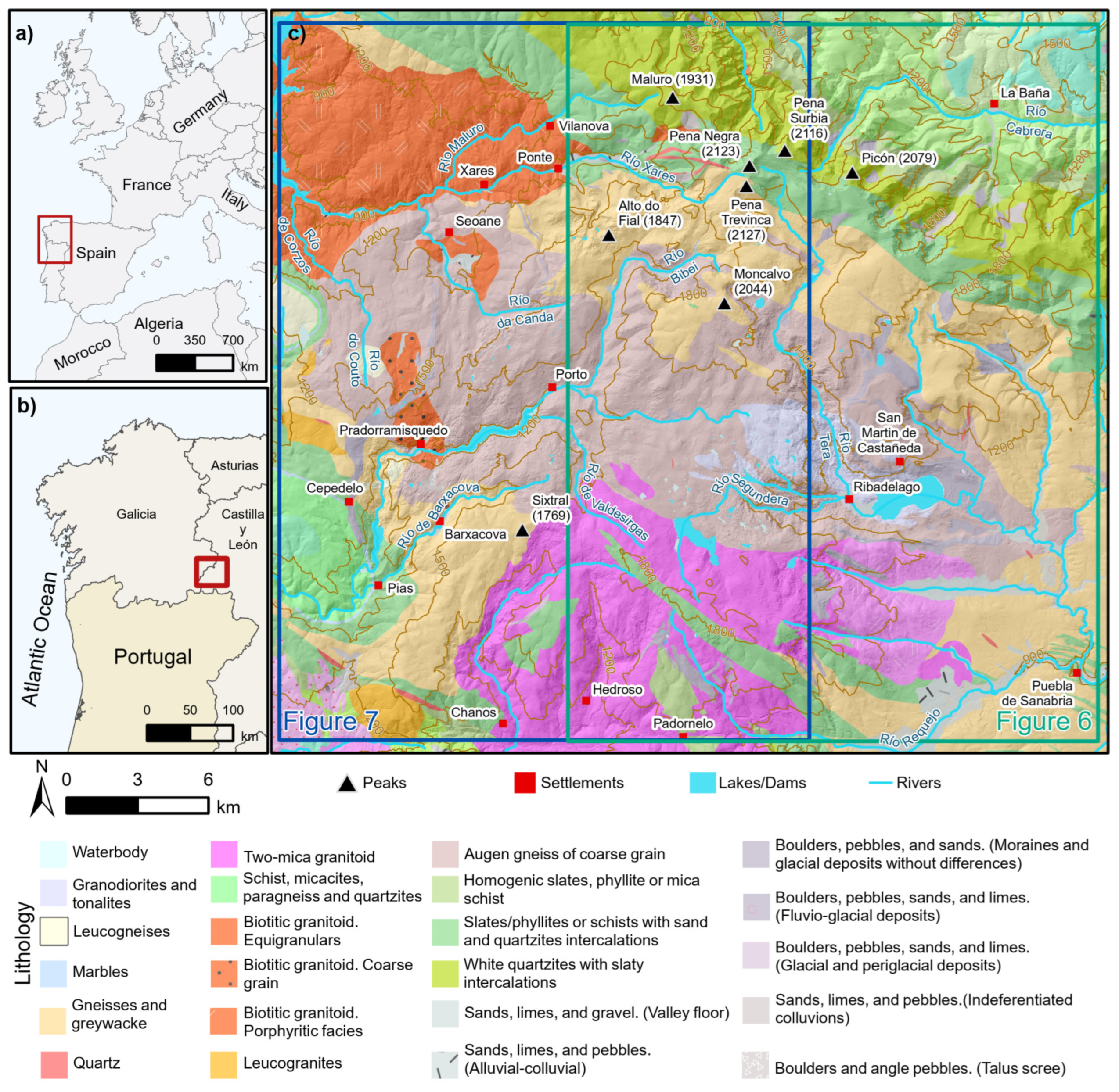
2. Study Area
3. Material and Methods
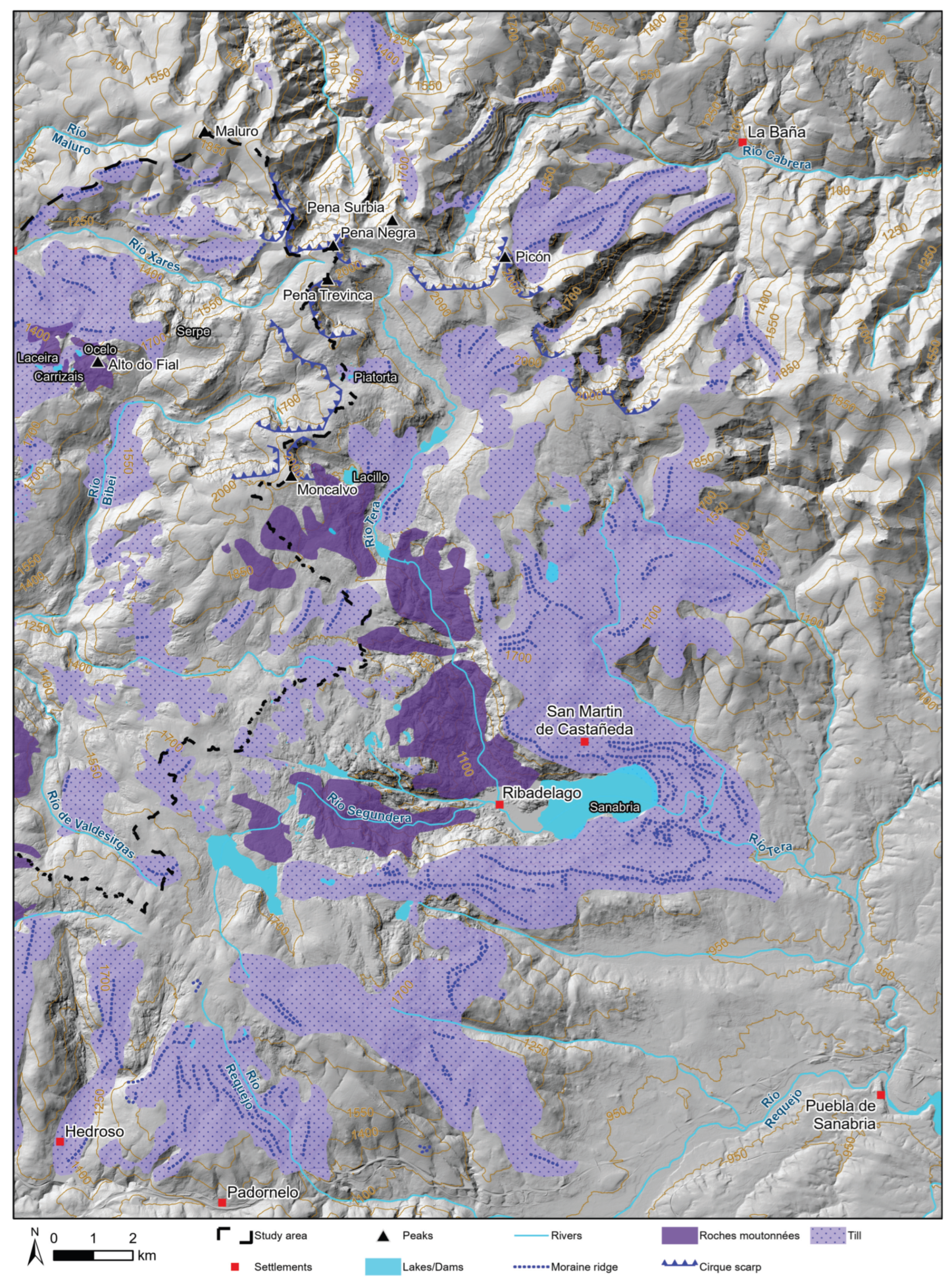
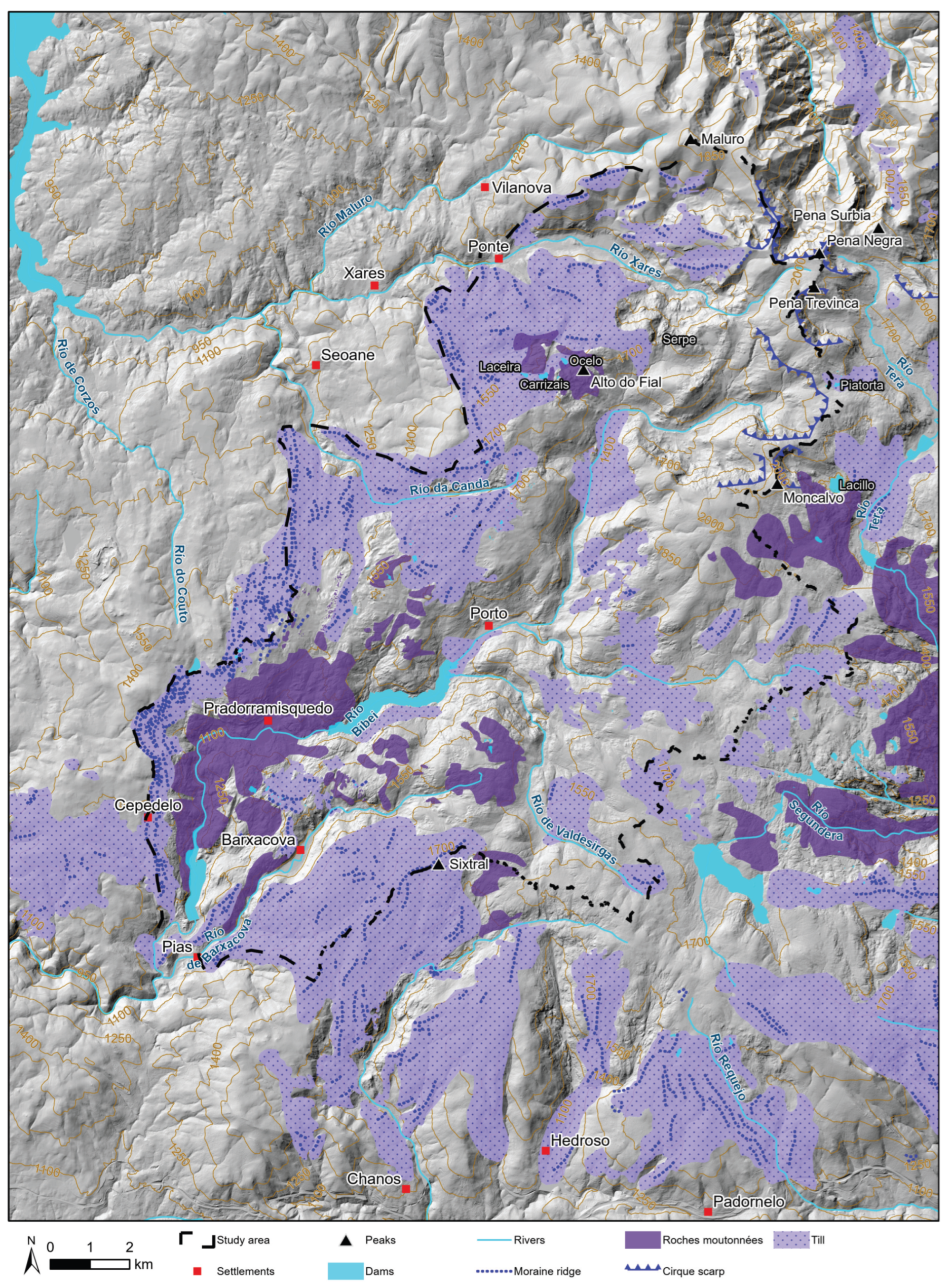
3.1. Mapping of Glacial Landforms and Deposits in the Trevinca Massif
3.2. The Glacial Development in the Western Sector of the Trevinca
3.2.1. Distribution of Moraine Ridges
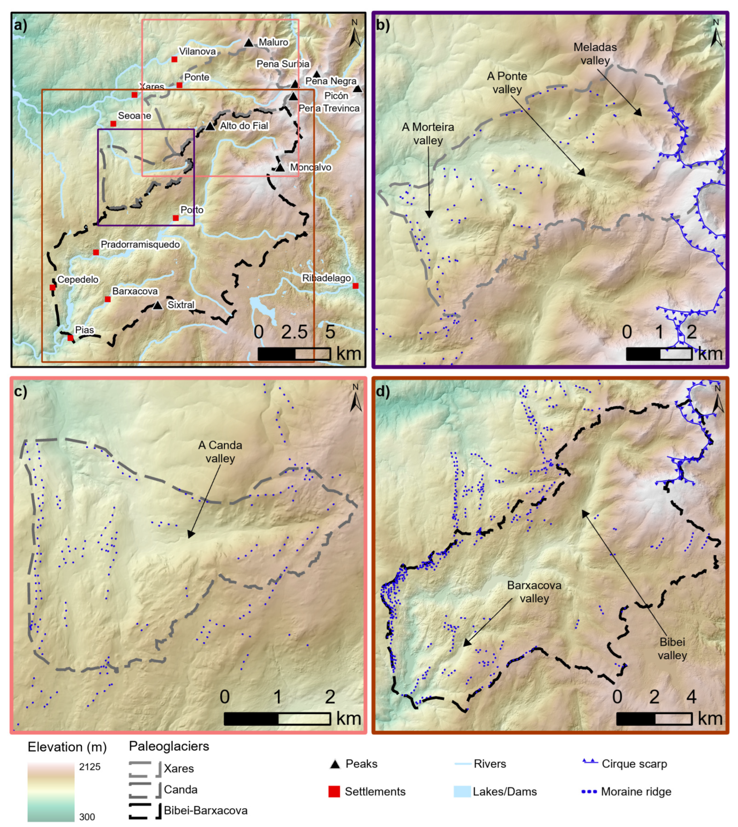
3.2.2. Basins/Paleobasins Delimitation
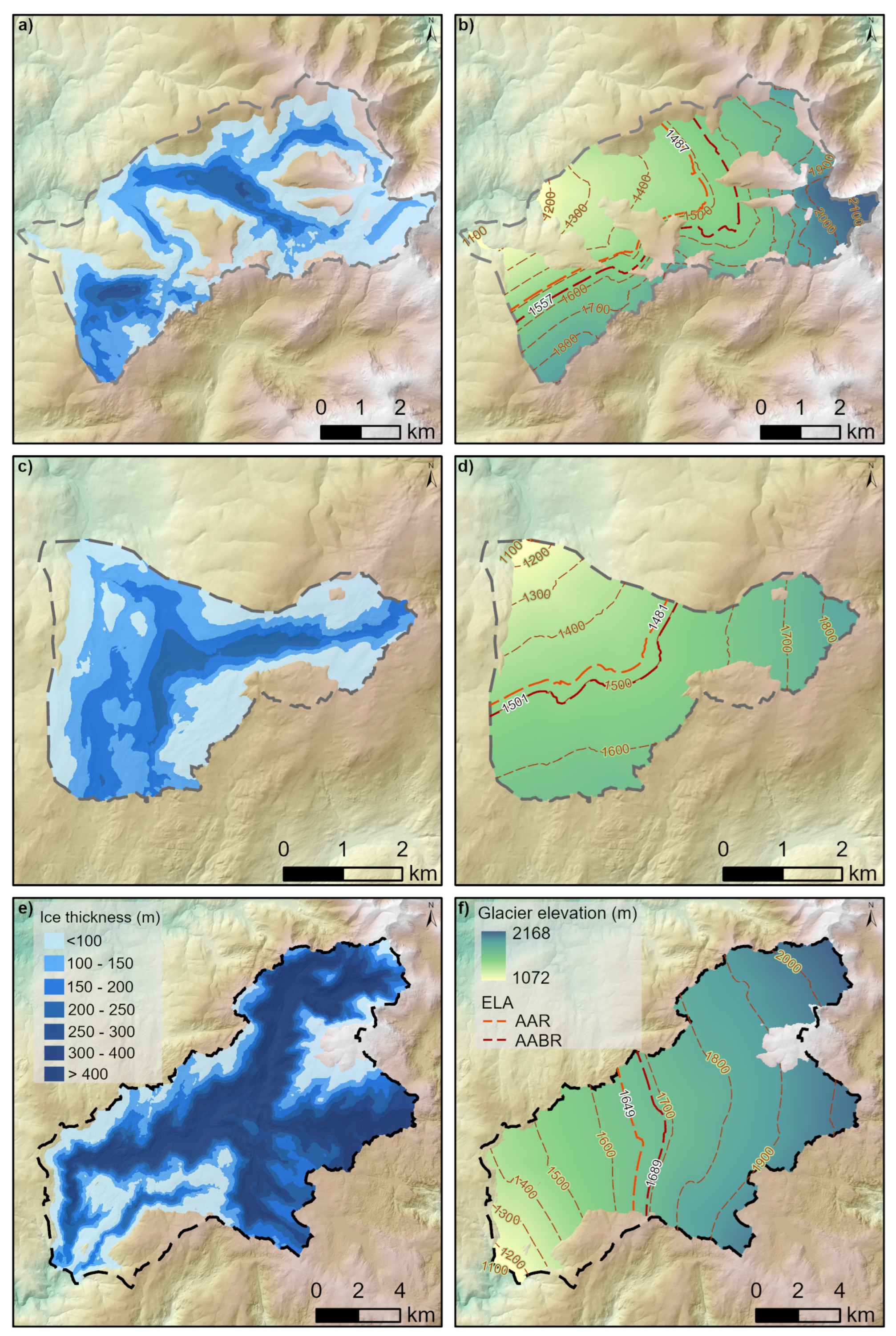
3.2.3. Paleoglacier Distribution and Ice Thickness
3.2.4. ELA Estimation
4. Results
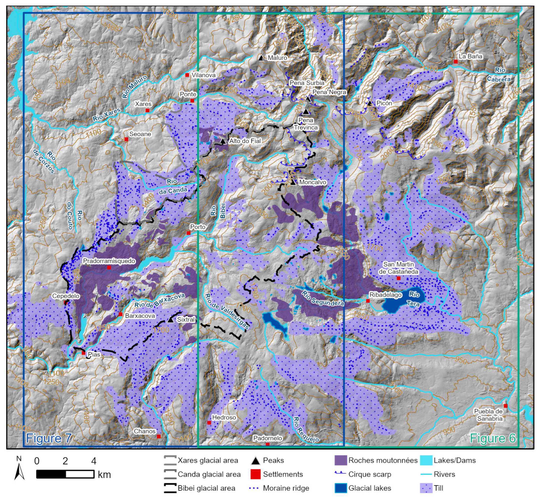
4.1. Glacial Cartography of Trevinca Massif
4.2. Definition and Main Characteristics of Occidental Paleoglaciers
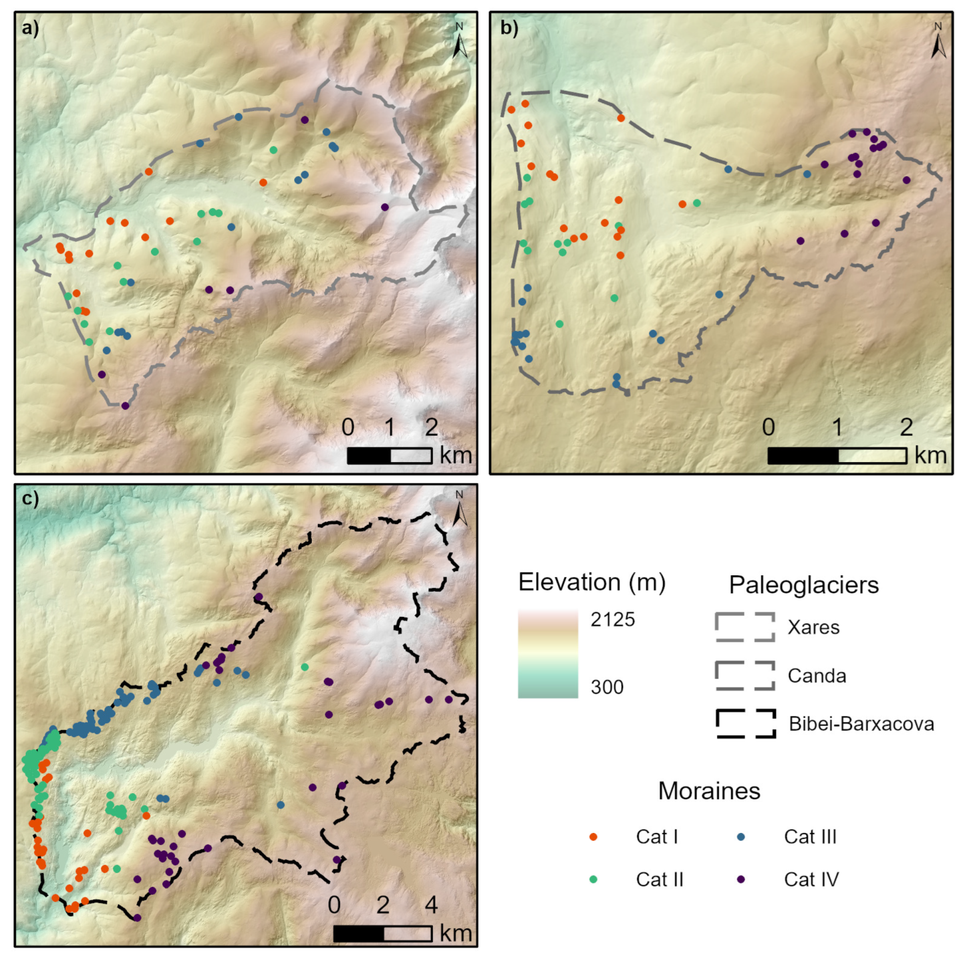
4.3. Moraine Ridges Distribution at the Occidental Sector
4.4. Relation between Moraine Ridges and the Glacial Phases
4.5. Paleoglacial Extension and Ice Thickness
4.6. ELA Estimation
5. Discussion
6. Conclusions
Author Contributions
Funding
Data Availability Statement
Acknowledgments
Conflicts of Interest
Abbreviations
| AABR | Area–altitude balance ratio |
| AAR | Accumulation area ratio |
| DEM | Digital elevation model |
| ELA | Equilibrium-line altitude |
| GIS | Geographic information system |
| gLGM | Global last glacial maximum |
| LiDAR | Light detection and ranging |
| lLGM | Local last glacial maximum |
| OSL | Optically stimulated luminescence |
| PNOA | Plan Nacional de Ortofotografía Aérea (Spain) |
References
- Oliva, M.; Palacios, D.; Fernández-Fernández, J.; Rodríguez-Rodríguez, L.; García-Ruiz, J.; Andrés, N.; Carrasco, R.; Pedraza, J.; Pérez-Alberti, A.; Valcárcel-Díaz, M.; et al. Late Quaternary glacial phases in the Iberian Peninsula. Earth-Sci. Rev. 2019, 192, 564–600. [Google Scholar] [CrossRef]
- Harris, C.; Arenson, L.U.; Christiansen, H.H.; Etzelmüller, B.; Frauenfelder, R.; Gruber, S.; Haeberli, W.; Hauck, C.; Hölzle, M.; Humlum, O.; et al. Permafrost and climate in Europe: Monitoring and modelling thermal, geomorphological and geotechnical responses. Earth-Sci. Rev. 2009, 92, 117–171. [Google Scholar] [CrossRef]
- Oliva, M.; Serrano, E.; Gómez-Ortiz, A.; González-Amuchastegui, M.; Nieuwendam, A.; Palacios, D.; Pérez-Alberti, A.; Pellitero-Ondicol, R.; Ruiz-Fernández, J.; Valcárcel-Díaz, M.; et al. Spatial and temporal variability of periglaciation of the Iberian Peninsula. Quat. Sci. Rev. 2016, 137, 176–199. [Google Scholar] [CrossRef]
- Sáenz Ridruejo, C. Varves glaciares del Alto Bibey. Rev. Obras Públicas 1968, 115, 339–350. [Google Scholar]
- Vandenberghe, J.; French, H.M.; Gorbunov, A.; Marchenko, S.; Velichko, A.A.; Jin, H.; Cui, Z.; Zhang, T.; Wan, X. The Last Permafrost Maximum (LPM) map of the Northern Hemisphere: Permafrost extent and mean annual air temperatures, 25–17 ka BP. Boreas 2014, 43, 652–666. [Google Scholar] [CrossRef]
- Pérez-Alberti, A.; Covelo Abeleira, P. Reconstrucción paleoambiental de la dinámica glaciar del Alto Bibei durante el Pleistoceno reciente a partir del estudio de los sedimentos acumulados en Pías (Noroeste de la Península Ibérica). In Dinámica y Evolución de Medios Cuaternarios; Xunta de Galicia: Santiago de Compostela, Spain, 1996; pp. 115–130. [Google Scholar]
- Viana-Soto, A.; Pérez-Alberti, A. Periglacial deposits as indicators of paleotemperatures. A case study in the Iberian Peninsula: The mountains of Galicia. Permafr. Periglac. Process. 2019, 30, 374–388. [Google Scholar] [CrossRef]
- Van Huissteden, K.; Vandenberghe, J.; Pollard, D. Palaeotemperature reconstructions of the European permafrost zone during marine oxygen isotope stage 3 compared with climate model results. J. Quat. Sci. 2003, 18, 453–464. [Google Scholar] [CrossRef]
- Benn, D.I.; Hulton, N.R.J. An ExcelTM spreadsheet program for reconstructing the surface profile of former mountain glaciers and ice caps. Comput. Geosci. 2010, 36, 605–610. [Google Scholar] [CrossRef]
- Fernández-Fernández, J.M. Aplicaciones de los sistemas de información geográfica en la reconstrucción paleoglaciar: El caso de la Sierra Segundera (Zamora, España). Geofocus Rev. Int. Cienc. Tecnol. Inf. Geográfica 2015, 16, 5. [Google Scholar]
- Pellitero, R.; Rea, B.R.; Spagnolo, M.; Bakke, J.; Ivy-Ochs, S.; Frew, C.R.; Hughes, P.; Ribolini, A.; Lukas, S.; Renssen, H. GlaRe, a GIS tool to reconstruct the 3D surface of palaeoglaciers. Comput. Geosci. 2016, 94, 77–85. [Google Scholar] [CrossRef]
- Oliva, M.; Palacios, D.; Fernández-Fernández, J.M. Iberia, Land of Glaciers How the Mountains Were Shaped by Glaciers; Elsevier: Amsterdam, The Netherlands, 2021; p. 300. [Google Scholar]
- García-Ruiz, J.M.; Palacios, D.; de Andrés, N.; Valero-Garcés, B.L.; López-Moreno, J.I.; Sanjuán, Y. Holocene and ‘little ice age’ glacial activity in the Marboré cirque, Monte Perdido Massif, Central Spanish Pyrenees. Holocene 2014, 24, 1439–1452. [Google Scholar] [CrossRef]
- Fernandes, M.; Oliva, M.; Vieira, G.; Palacios, D.; Fernández-Fernández, J.M.; Delmas, M.; García-Oteyza, J.; Schimmelpfennig, I.; Ventura, J. Maximum glacier extent of the Penultimate Glacial Cycle in the Upper Garonne Basin (Pyrenees): New chronological evidence. Environ. Earth Sci. 2021, 80, 1–20. [Google Scholar] [CrossRef]
- Serrano, E.; González-Trueba, J.J.; Pellitero, R.; Gómez-Lende, M. Quaternary glacial history of the Cantabrian Mountains of northern Spain: A new synthesis. Geol. Soc. Lond. Spec. Publ. 2016, 433, 55–85. [Google Scholar] [CrossRef]
- Serrano, E.; González-Trueba, J.; Pellitero, R.; González-García, M.; Gómez-Lende, M. Quaternary glacial evolution in the Central Cantabrian Mountains (Northern Spain). Geomorphology 2013, 196, 65–82. [Google Scholar] [CrossRef]
- Pisabarro, A.; Pellitero, R.; Serrano, E.; Gómez-Lende, M.; González-Trueba, J. Ground temperatures, landforms and processes in an Atlantic mountain. Cantabrian Mountains (Northern Spain). Catena 2017, 149, 623–636. [Google Scholar] [CrossRef]
- Ruiz-Fernández, J.; Oliva, M.; Cruces, A.; Lopes, V.; da Conceição Freitas, M.; Andrade, C.; Garcia-Hernandez, C.; López-Sáez, J.A.; Geraldes, M. Environmental evolution in the Picos de Europa (Cantabrian Mountains, SW Europe) since the last glaciation. Quat. Sci. Rev. 2016, 138, 87–104. [Google Scholar] [CrossRef]
- Palacios, D.; Gómez-Ortiz, A.; Alcalá-Reygosa, J.; Andrés, N.; Oliva, M.; Tanarro, L.M.; Salvador-Franch, F.; Schimmelpfennig, I.; Fernández-Fernández, J.M.; Léanni, L. The challenging application of cosmogenic dating methods in residual glacial landforms: The case of Sierra Nevada (Spain). Geomorphology 2019, 325, 103–118. [Google Scholar] [CrossRef]
- Palma, P.; Oliva, M.; García-Hernández, C.; Gómez Ortiz, A.; Ruiz-Fernández, J.; Salvador-Franch, F.; Catarineu, M. Spatial characterization of glacial and periglacial landforms in the highlands of Sierra Nevada (Spain). Sci. Total Environ. 2017, 584–585, 1256–1267. [Google Scholar] [CrossRef] [PubMed]
- Stickel, R. Observaciones de Morfología Glaciar en el No de España. Bol. R. Soc. Esp. Hist. Nat. 1929, 29, 297–318. [Google Scholar]
- Schmitz, H. Glazialmorphologische Untersuchungen im Bergland Nordwestspaniens (Galicien/León); Kolner Geogr. Arb. 23; Univ. Köln: Köln, Germany, 1969. [Google Scholar]
- Pérez-Alberti, A. Nuevas observaciones sobre glaciarismo y periglaciarismo en el NW de la Península ibérica: La Galicia sudoriental. Acta GeolóGica HispáNica 1979, 14, 441–444. [Google Scholar]
- Hall-Riaza, J.F.; Valcárcel, M.; Blanco-Chao, R. Caracterización morfométrica de formas glaciares en cuña en las Sierras de Xistral, Teleno y Cabrera. Polígonos. Rev. Geogr. 2016, 28, 55. [Google Scholar] [CrossRef]
- Azor, A.; González Lodeiro, F.; Hacar Rodríguez, M.; Martín Parra, L.M.; Martínez Catalán, J.R.; Pérez Estaún, A. Estratigrafía y estructura del Paelozoico en el Dominio del Ollo de Sapo. In Proceedings of the Paleozoico Inferior de Ibero-América. Conferencia Internacional sobre el Paleozoico Inferior de Ibero-América, Mérida, Spain, 6–12 May 1992; pp. 469–483. [Google Scholar]
- Vidal Romaní, J.R.; Marti, K. The glaciation of Serra de Queixa-Invernadoiro and Serra do Gerês-Xurés, NW Iberia. A critical review and a cosmogenic nuclide (10Be and 21 Ne) chronology. Cad. Lab. Xeolóxico de Laxe. Rev. Xeoloxía Galega Hercínico Penins. 2015, 38, 25–43. [Google Scholar] [CrossRef]
- Valcárcel-Díaz, M.; Pérez-Alberti, A. Un ejemplo de glaciarismo de baja cota en el NW de la Península Ibérica: El valle de Queixadoiro. In Estudios Recientes en Geomorfología. Patrimonio, Montaña y dináMica Territorial; Universidad de Valladolid: Valladolid, Spain, 2002; Volume 205, p. 215. [Google Scholar]
- Hernández-Pacheco, F. El glaciarismo cuaternario de la Sierra de Queija-Orense, Galicia. Bol. R. Soc. Esp. Hist. Nat. 1957, 55, 27–74. [Google Scholar]
- Rodríguez-Guitián, M.; Pérez-Alberti, A.; Valcárcel-Díaz, M. El modelado glaciar en la vertiente oriental de la sierra de Ancares (noroeste de la Península Ibérica). Papeles Geogr. 1992, 18, 39–54. [Google Scholar]
- Valcárcel Díaz, M.; Rodríguez Guitián, M.; Pérez Alberti, A. Dinámica glaciar pleistocena del complejo Porcarizas-Valongo (Serra dos Ancares, NW Ibérico). In Avances en el Conocimiento Paleoambiental de las Montañas Lucenses; Diputación de Lugo: Lugo, Spain, 1996; pp. 53–64. [Google Scholar]
- Llopis Lladó, N. Sobre la morfología de los picos Ancares y Miravalles. An. Asoc. Española Prog. Cienc. (Rev. Las Cienc.) 1954, 19, 627–643. [Google Scholar]
- Kossel, U. Problemas geomorfológicos acerca de la determinación del máximo avance glaciar en la Sierra de Ancares (León-Lugo-Asturias). In Dinámica y Evolución de Medios Cuaternarios; Xunta de Galicia: Santiago de Compostela, Spain, 1996; Volume 131, p. 142. [Google Scholar]
- Pérez-Alberti, A. El patrimonio glaciar y periglaciar del Geoparque Mundial UNESCO Montañas do Courel (Galicia). Cuaternario Geomorfol. 2021, 35, 79–98. [Google Scholar] [CrossRef]
- Vidal-Romaní, J.; Aira-Rodríguez, M.; Santos Fidalgo, L. La glaciación finicuaternaria en el NO de la Península Ibérica (Serra do Courel, Lugo): Datos geomorfológicos y paleobotánicos. In Libro de Resúmenes. VIII Reunión Nacional Sobre el Cuaternario; Universidad de Valencia: Valencia, Spain, 1991. [Google Scholar]
- Aira, M.J.; Guitian Ojea, F. Contribución al estudio de los suelos y sedimentos de montaña de Galicia y su cronología por analisis polinico. I. Sierra del Caurel (Lugo). An. Edafol. Agrobiol. 1986, 45, 1189–1202. [Google Scholar]
- Rodríguez-Guitián, M.A.; Valcárcel-Díaz, M. Contribución al conocimiento del glaciarismo pleistoceno en la vertiente sur-occidental del Macizo de Peña Trevinca (Montañas Galaico-Sanabrienses, NW Ibérico). In Proceedings of the Geomorfología de España, Logroño, Spain, 14–16 September 1994. [Google Scholar]
- Dionne, J.; Pérez-Alberti, A. Observations of vertical cylindrical structures in an unconsolidated Quaternary deposit, in Spain. Geogr. Phys. Quat. 2001, 54, 343–349. [Google Scholar]
- Rodríguez-Rodríguez, L.; Domínguez-Cuesta, M.J.; Jimenez Sánchez, M. Reconstrucción en 3D del máximo glaciar registrado en la cuenca del Lago de Sanabria (Noroeste de España). Boletín Real Soc. Española Hist. Nat. (Sección Geol.) 2011, 105, 31–44. [Google Scholar]
- Rodríguez-Rodríguez, L.; Jiménez-Sánchez, M.; Domínguez-Cuesta, M.J.; González-Lemos, S. The glaciers around Lake Sanabria. In Iberia, Land of Glaciers; Elsevier: Amsterdam, The Netherlands, 2022; pp. 335–351. [Google Scholar]
- Pérez-Alberti, A.; Valcárcel-Díaz, M. Chapter 4.14—The glaciers in Eastern Galicia. In Iberia, Land of Glaciers; Oliva, M., Palacios, D., Fernández-Fernández, J.M., Eds.; Elsevier: Amsterdam, The Netherlands, 2022; pp. 375–395. [Google Scholar] [CrossRef]
- Valcarcel-Díaz, M.; Pérez-Alberti, A. Chapter 4.13—The glaciers in Western Galicia. In Iberia, Land of Glaciers; Oliva, M., Palacios, D., Fernández-Fernández, J.M., Eds.; Elsevier: Amsterdam, The Netherlands, 2022; pp. 353–373. [Google Scholar] [CrossRef]
- Oliva, M.; Serrano, E.; Fernández-Fernández, J.M.; Palacios, D.; Fernandes, M.; García-Ruiz, J.M.; López-Moreno, J.I.; Pérez-Alberti, A.; Antoniades, D. The Iberian Peninsula. In Periglacial Landscapes of Europe; Oliva, M., Nývlt, D., Fernández-Fernández, J.M., Eds.; Springer International Publishing: Cham, Switzerland, 2022; pp. 43–68. [Google Scholar] [CrossRef]
- Pérez-Alberti, A.; Valcárcel-Díaz, M.; Martini, P.I.; Pascucci, V.; Andreucci, S. Upper Pleistocene glacial valley-junction sediments at Pias, Trevinca Mountains, NW Spain. Geol. Soc. Lond. Spec. Publ. 2011, 354, 93–110. [Google Scholar] [CrossRef]
- Díez-Montes, A. La geología del Dominio “Ollo de Sapo” en las comarcas de Sanabria y Terra do Bolo. Ph.D. Thesis, University of Salamanca, Salamanca, Spain, 2006. [Google Scholar]
- Muñoz-Martín, A.; Álvarez, J.; Carbó, A.; De Vicente, G.; Vegas, R.; Cloetingh, S. La Estructura de la Corteza del Antepaís Ibérico; Geología de España; SGE-IGME: Madrid, Spain, 2004; pp. 591–596. [Google Scholar]
- Pérez-Alberti, A. Climatoloxía. In Xeografía de Galicia; Pérez-Alberti, A., Ed.; Sálvora: A Coruña, Spain, 1982. [Google Scholar]
- Meteogalicia. Meteogalicia. 2023. Available online: https://www.meteogalicia.gal/ (accessed on 3 January 2023).
- IGN. Instituto Geográfico Nacional. 2023. Available online: https://www.centrodedescargas.cnig.es/ (accessed on 2 January 2023).
- Lambiel, C.; Maillard, B.; Regamei, B.; Martin, S.; Kummert, M.; Schoeneich, P.; Pellitero Ondicol, R.; Reynard, E. Adaptation of the geomorphological mapping system of the University of Lau sanne for ArcGIS. In Proceedings of the 8th International Conference on Geomorphology (IAG), Paris, France, 27–31 August 2013. [Google Scholar]
- Jenks, G.F. The data model concept in statistical mapping. Int. Yearb. Cartogr. 1967, 7, 186–190. [Google Scholar]
- R Core Team. R: A Language and Environment for Statistical Computing; R Core Team: Vienna, Austria, 2021. [Google Scholar]
- Temovski, M.; Madarász, B.; Kern, Z.; Milevski, I.; Ruszkiczay-Rüdiger, Z. Glacial geomorphology and Preliminary glacier reconstruction in the Jablanica mountain, Macedonia, central Balkan peninsula. Geosciences 2018, 8, 270. [Google Scholar] [CrossRef]
- Oien, R.; Spagnolo, M.; Rea, B.; Barr, I.; Bingham, R.G.; Jansen, J. Analysing palaeo cirque glacier equilibrium line altitudes as indicators of palaeoclimate across Scandinavia. In Proceedings of the EGU General Assembly 2020, Online, 4–8 May 2020. [Google Scholar]
- Paul, O.J.; Dar, R.A.; Romshoo, S.A. Paleo-glacial and paleo-equilibrium line altitude reconstruction from the Late Quaternary glacier features in the Pir Panjal Range, NW Himalayas. Quat. Int. 2021, 642, 5–16. [Google Scholar] [CrossRef]
- Campos, N.; Palacios, D.; Tanarro, L.M. Glacier reconstruction of La Covacha Massif in Sierra de Gredos (central Spain) during the Last Glacial Maximum. J. Mt. Sci. 2019, 16, 1336–1352. [Google Scholar] [CrossRef]
- Moulin, A.; Benedetti, L.; Vidal, L.; Hage-Hassan, J.; Elias, A.; Van der Woerd, J.; Schimmelpfennig, I.; Daëron, M.; Tapponnier, P. LGM glaciers in the SE Mediterranean? First evidence from glacial landforms and 36Cl dating on Mount Lebanon. Quat. Sci. Rev. 2022, 285, 107502. [Google Scholar] [CrossRef]
- Palacios, D.; Rodríguez-Mena, M.; Fernández-Fernández, J.M.; Schimmelpfennig, I.; Tanarro, L.M.; Zamorano, J.J.; Andrés, N.; Úbeda, J.; Sæmundsson, T.; Brynjólfsson, S. Reversible glacial-periglacial transition in response to climate changes and paraglacial dynamics: A case study from Héðinsdalsjökull (northern Iceland). Geomorphology 2021, 388, 107787. [Google Scholar] [CrossRef]
- Figueira, E.; Gomes, A.; Pérez-Alberti, A.; Chaminé, H.I. 3D modelling of the maximum ice extent and thickness of the palaeoglacier of Serra do Soajo, Northern Portugal. In Proceedings of the 10th International Conference on Geomorphology, Coimbra, Portugal, 12–16 September 2022. [Google Scholar] [CrossRef]
- Pellitero, R.; Rea, B.R.; Spagnolo, M.; Bakke, J.; Hughes, P.; Ivy-Ochs, S.; Lukas, S.; Ribolini, A. A GIS tool for automatic calculation of glacier equilibrium-line altitudes. Comput. Geosci. 2015, 82, 55–62. [Google Scholar] [CrossRef]
- Pérez-Alberti, A.; Valcárcel Díaz, M.; Blanco-Chao, R. Pleistocene glaciation in Spain. In Quaternary Glaciations–Extent and Chronology. Part I: Europe. Amsterdam, etc.; Developments in Quaternary Science 2; Elsevier: Amsterdam, The Netherlands, 2004. [Google Scholar]
- Pérez-Alberti, A.; Rodríguez-Guitián, M.; Valcárcel-Díaz, M. Las Formas y Depósitos Glaciares en las Sierras Orientales y Septentrionales de Galicia (NW Península Ibérica); Xunta de Galicia: A Coruña, Spain, 1993; pp. 61–90. [Google Scholar]
- Rodríguez-Rodríguez, L.; Jiménez-Sánchez, M.; Domínguez-Cuesta, M.J.; Rinterknecht, V.; Pallàs, R.; Bourlès, D.; Valero-Garcés, B. A multiple dating-method approach applied to the Sanabria Lake moraine complex (NW Iberian Peninsula, SW Europe). Quat. Sci. Rev. 2014, 83, 1–10. [Google Scholar] [CrossRef]
- Vidal Romaní, J.R.; Fernández-Mosquera, D. Glaciarismo Pleistoceno en el NW de la peninsula Ibérica (Galicia, España-Norte de Portugal). Enseñanza Las Cienc. Tierra 2005, 13, 270–277. [Google Scholar]
- Martínez Cortizas, A.; Moares Domínguez, M.M.; Pérez-Alberti, A. Los Procesos Periglaciares en el Noroeste de la Península Ibérica; Universidad de Granada: Granada, Spain, 1994; pp. 33–54. [Google Scholar]
- Fernández-Duro, C. El Lago de Sanabria o de San Martín de Castañeda. Bol. Real Soc. Geogr. 1879, 6, 65. [Google Scholar]
- Taboada, J. El lago de San Martín de Castañeda. Bol. Soc. Esp. Hist. Nat. 1913, 13, 860–883. [Google Scholar]
- Pérez-Alberti, A. Procesos periglaciares e glaciares no Nordeste de Galicia. Rev. Terra 1983, 3, 78–86. [Google Scholar]
- Pérez-Alberti, A. La Geomorfología de la Galicia Sudoriental: Problemas Geomorfológicos de un Macizo Hercínico de la Fachada atlántica Ibérica: Centro-Sudeste de Galicia. Ph.D. Thesis, Universidade de Santiago de Compostela, A Coruña, Spain, 1990. [Google Scholar]
- Luque, J.A. El Lago de Sanabria: Un Sensor de Las Oscilaciones Climáticas del Atlántico Norte Durante Los últimos 6.000 Años; Universitat de Barcelona: Barcelona, Spain, 2003. [Google Scholar]
- Rico, M.T.; Valero-Garcés, B.L.; Vega, J.C.; Moreno Caballud, A.; González-Sampériz, P.; Morellón, M.; Mata, M.P. El Registro Sedimentario del Lago de Sanabria Desde la última Deglaciación; Asociación Española para el Estudio del Cuaternario; Universidad Politécnica de Madrid: Madrid, Spain, 2007. [Google Scholar]
- Jambrina-Enríquez, M.; Rico, M.; Moreno, A.; Leira, M.; Bernárdez, P.; Prego, R.; Recio, C.; Valero-Garcés, B.L. Timing of deglaciation and postglacial environmental dynamics in NW Iberia: The Sanabria Lake record. Quat. Sci. Rev. 2014, 94, 136–158. [Google Scholar] [CrossRef]
- Jambrina-Enríquez, M.; Recio, C.; Vega, J.C.; Valero-Garcés, B. Tracking climate change in oligotrophic mountain lakes: Recent hydrology and productivity synergies in Lago de Sanabria (NW Iberian Peninsula). Sci. Total Environ. 2017, 590, 579–591. [Google Scholar] [CrossRef] [PubMed]
- Cowton, T.; Hughes, P.D.; Gibbard, P.L. Palaeoglaciation of Parque Natural Lago de Sanabria, northwest Spain. Geomorphology 2009, 108, 282–291. [Google Scholar] [CrossRef]
- Rodríguez-Rodríguez, L.; Jiménez-Sánchez, M.; Domínguez-Cuesta, M.J.; Rico, M.T.; Valero-Garcés, B. Last deglaciation in northwestern Spain: New chronological and geomorphologic evidence from the Sanabria region. Geomorphology 2011, 135, 48–65. [Google Scholar] [CrossRef]
- Vieira, G. Combined numerical and geomorphological reconstruction of the Serra da Estrela plateau icefield, Portugal. Geomorphology 2008, 97, 190–207. [Google Scholar] [CrossRef]
- Hernández-Pacheco, F. Huellas Glaciares en la Sierra de Queija (Orense). Bol. R. Soc. Esp. Hist. Nat. 1949, 47, 97–102. [Google Scholar]
- Ribolini, A.; Bini, M.; Isola, I.; Spagnolo, M.; Zanchetta, G.; Pellitero, R.; Mechernich, S.; Gromig, R.; Dunai, T.; Wagner, B.; et al. An Oldest Dryas glacier expansion on Mount Pelister (Former Yugoslavian Republic of Macedonia) according to 10Be cosmogenic dating. J. Geol. Soc. 2017, 175, 100–110. [Google Scholar] [CrossRef]
- Spagnolo, M.; Ribolini, A. Glacier extent and climate in the Maritime Alps during the Younger Dryas. Palaeogeogr. Palaeoclimatol. Palaeoecol. 2019, 536, 109400. [Google Scholar] [CrossRef]
- Valcárcel-Díaz, M.; Blanco-Chao, R.; Martínez-Cortizas, A.; Pérez-Alberti, A. Estimation of paleotemperatures in Galicia during the last glacial cycle from geomorphological and climatic data. In Investigaciones Recientes de la Geomorfología Española; Gómez-Ortiz, A., Salvador Franch, F., Eds.; Universitat de Barcelona: Barcelona, Spain, 1998; pp. 661–664. [Google Scholar]
- Bordonau, J.; Serrat, D.; Vilaplana, J.M. Las fases glaciares cuaternarias en los Pirineos. In The Late Quaternary in the Western Pyrenean Region; Servicio Editorial Universidad del País Vasco: Bilbao, Spain, 1992; pp. 303–312. [Google Scholar]
- Martínez de Pisón, E.; Serrano, E. Morfología Glaciar del valle del Tena (Pirineo Aragonés). In Las Huellas Glaciares de las Montañas españOlas; Servicio de Publicaciones e Intercambio Científico: A Coruña, Spain, 1998; pp. 239–261. [Google Scholar]


| Basin | Surface (ha) | Max. Elevation (m) | Min. Elevation (m) | Mean Elevation (m) |
|---|---|---|---|---|
| Xares | 3764.05 | 2123.92 | 1089.2 | 1522.91 |
| Bibei-Barxacova | 15,879.94 | 2049.55 | 997.20 | 1532.12 |
| Canda | 1650.52 | 1750.07 | 1069.33 | 1420.82 |
| Category | Maximum Elevation (m) | Number of Moraines |
|---|---|---|
| I | 1339.81 | 62 |
| II | 1459.04 | 92 |
| III | 1593.67 | 91 |
| IV | 1933.24 | 55 |
| Bibei-Barxacova | Xares | Canda | |||||||
|---|---|---|---|---|---|---|---|---|---|
| Category | Elevation (m) | Number of Moraines | Percentage | Elevation (m) | Number of Moraines | Percentage | Elevation (m) | Number of Moraines | Percentage |
| I | 1342.77 | 31 | 15.98 | 1263.02 | 8 | 17.39 | 1288.60 | 7 | 11.67 |
| II | 1462.54 | 69 | 35.57 | 1406.46 | 14 | 30.43 | 1425.36 | 22 | 36.67 |
| III | 1576.71 | 59 | 30.41 | 1575.65 | 18 | 39.13 | 1566.52 | 16 | 26.67 |
| IV | 1784.99 | 35 | 18.04 | 1933.24 | 6 | 13.04 | 1735.00 | 15 | 25.00 |
| Paleoglacier | Max. Thickness (m) | Mean Thickness (m) | Extension (km) | Length (km) |
|---|---|---|---|---|
| Xares | 292.51 | 101.97 | 28.26 | 7.83 |
| Canda | 384.54 | 116.60 | 14.85 | 6.59 |
| Bibei-Barxacova | 527.03 | 218.16 | 143.74 | 27.26 |
| Paleoglacier | ELA (m) | |||||
|---|---|---|---|---|---|---|
| AABR | AABR (1.75) | AAR | AAR (0.67) | MGE | AA | |
| Xares | 1487–1617 | 1557 | 1427–1657 | 1487 | 1597 | 1604 |
| Canda | 1451–1531 | 1501 | 1431–1571 | 1481 | 1551 | 1528 |
| Bibei-Barxacova | 1599–1749 | 1689 | 1569–1839 | 1649 | 1789 | 1735 |
Disclaimer/Publisher’s Note: The statements, opinions and data contained in all publications are solely those of the individual author(s) and contributor(s) and not of MDPI and/or the editor(s). MDPI and/or the editor(s) disclaim responsibility for any injury to people or property resulting from any ideas, methods, instructions or products referred to in the content. |
© 2023 by the authors. Licensee MDPI, Basel, Switzerland. This article is an open access article distributed under the terms and conditions of the Creative Commons Attribution (CC BY) license (https://creativecommons.org/licenses/by/4.0/).
Share and Cite
Pérez-Alberti, A.; Gómez-Pazo, A. Glaciers Landscapes during the Pleistocene in Trevinca Massif (Northwest Iberian Peninsula). Land 2023, 12, 530. https://doi.org/10.3390/land12030530
Pérez-Alberti A, Gómez-Pazo A. Glaciers Landscapes during the Pleistocene in Trevinca Massif (Northwest Iberian Peninsula). Land. 2023; 12(3):530. https://doi.org/10.3390/land12030530
Chicago/Turabian StylePérez-Alberti, Augusto, and Alejandro Gómez-Pazo. 2023. "Glaciers Landscapes during the Pleistocene in Trevinca Massif (Northwest Iberian Peninsula)" Land 12, no. 3: 530. https://doi.org/10.3390/land12030530
APA StylePérez-Alberti, A., & Gómez-Pazo, A. (2023). Glaciers Landscapes during the Pleistocene in Trevinca Massif (Northwest Iberian Peninsula). Land, 12(3), 530. https://doi.org/10.3390/land12030530