
Contribution of High-Resolution Virtual Outcrop Models for the Definition of Rockfall Activity and Associated Hazard Modelling

 , ,
, ,  , , and
Abstract
1. Introduction
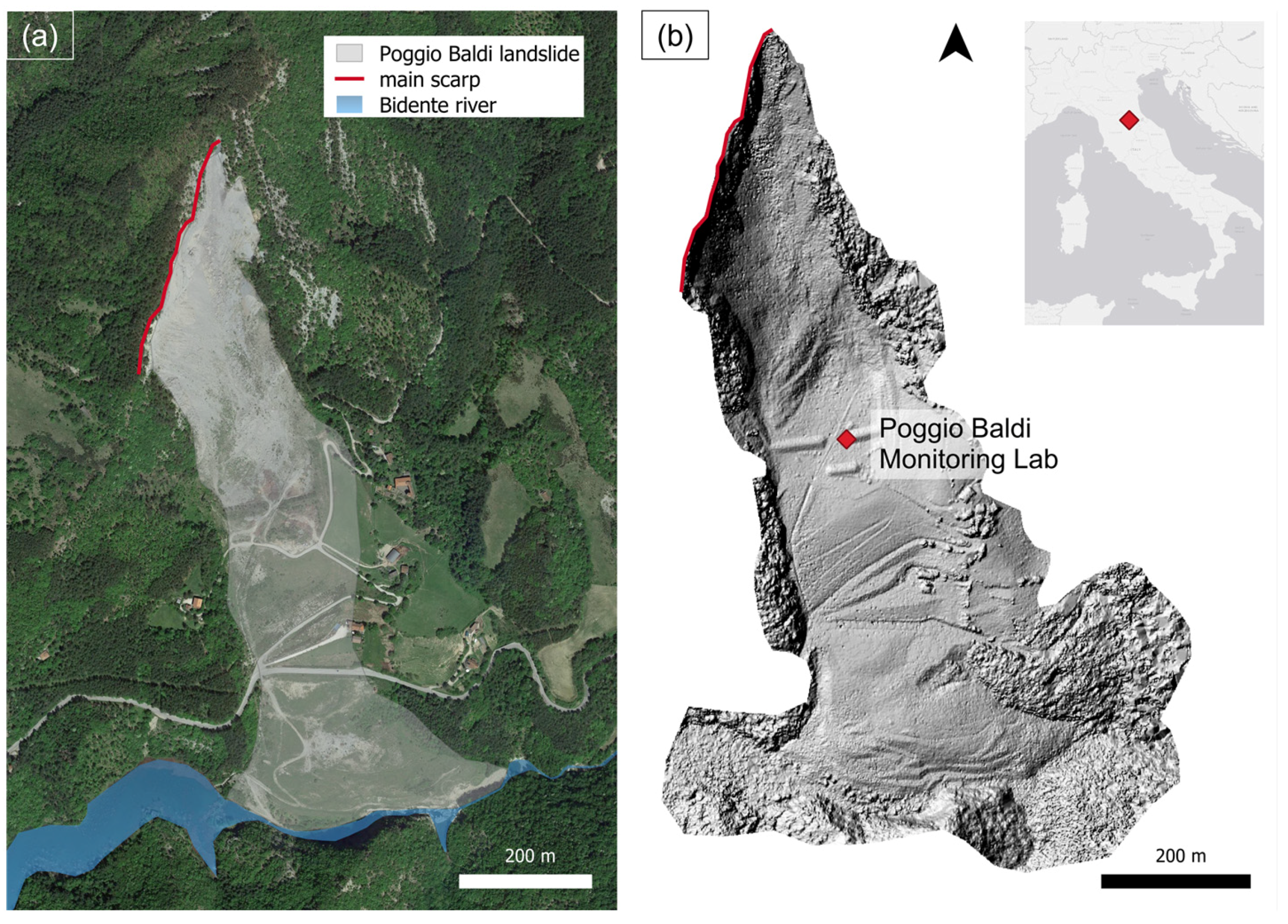
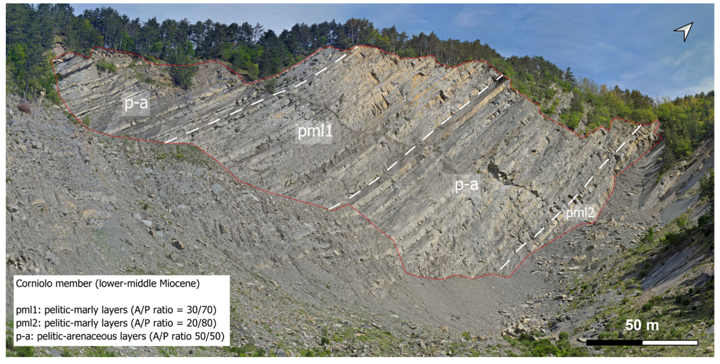
2. Study Area
3. Material and Methods
3.1. Virtual Outcrop Models
3.2. Slope Analysis
Rockfall Hazard Analysis and Numerical Modelling
4. Results
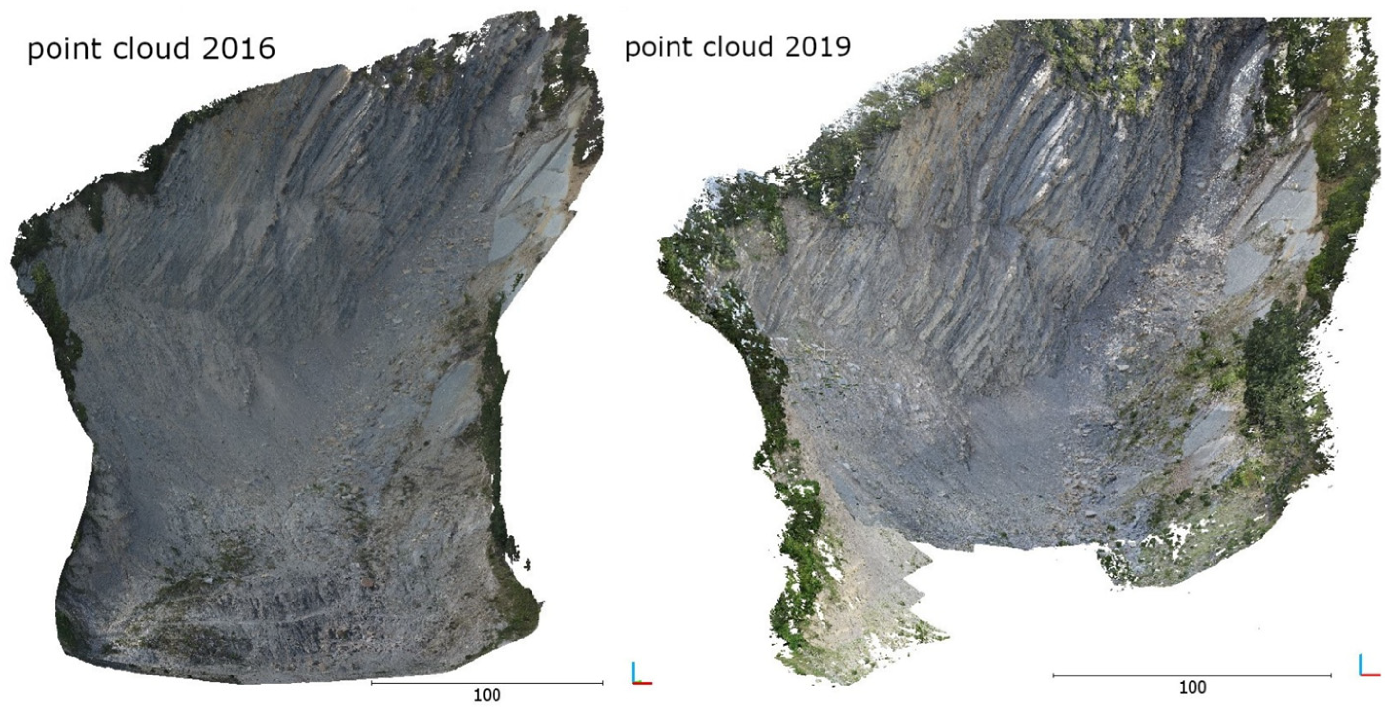
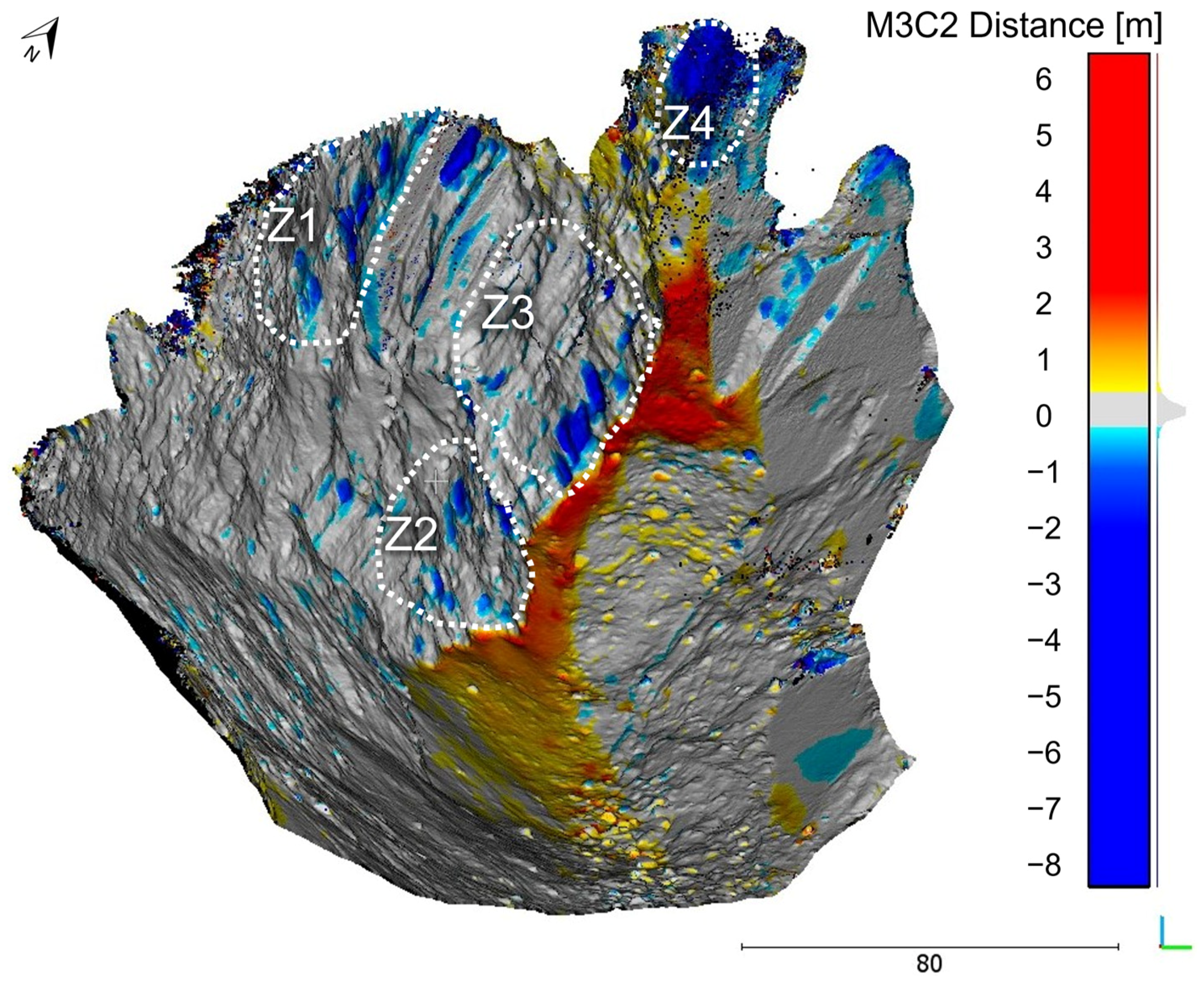
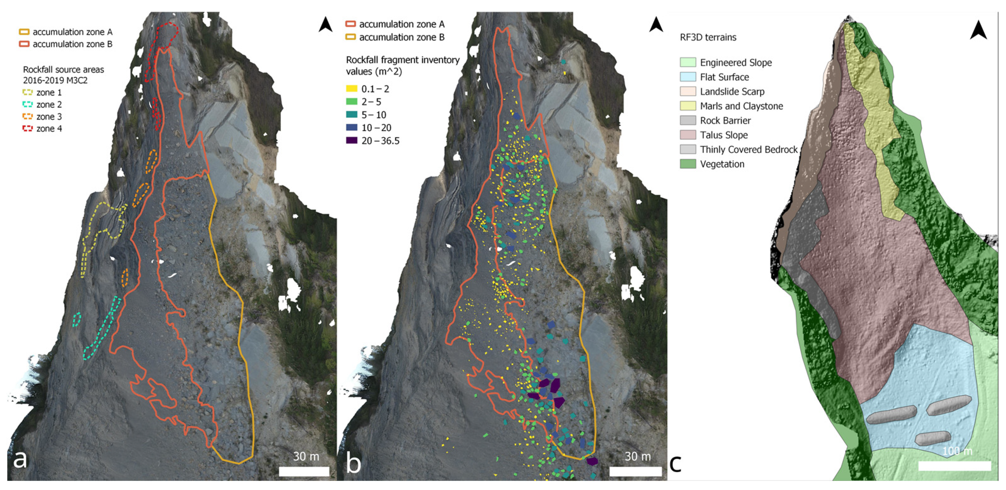
4.1. Three-Dimensional Change Detection
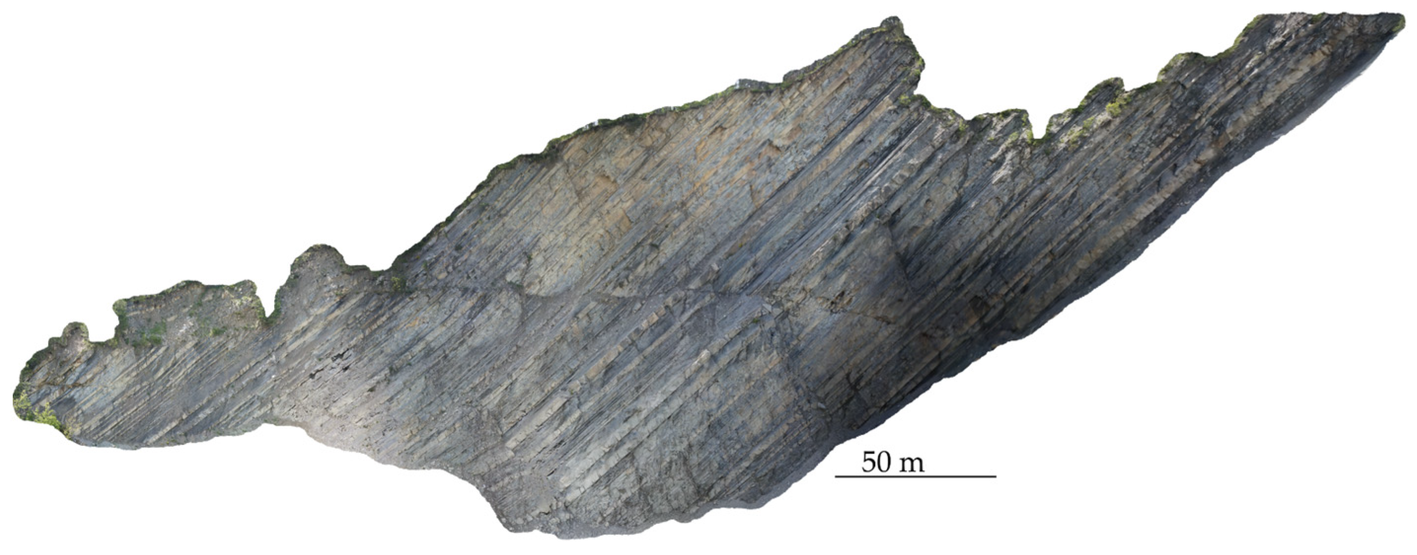
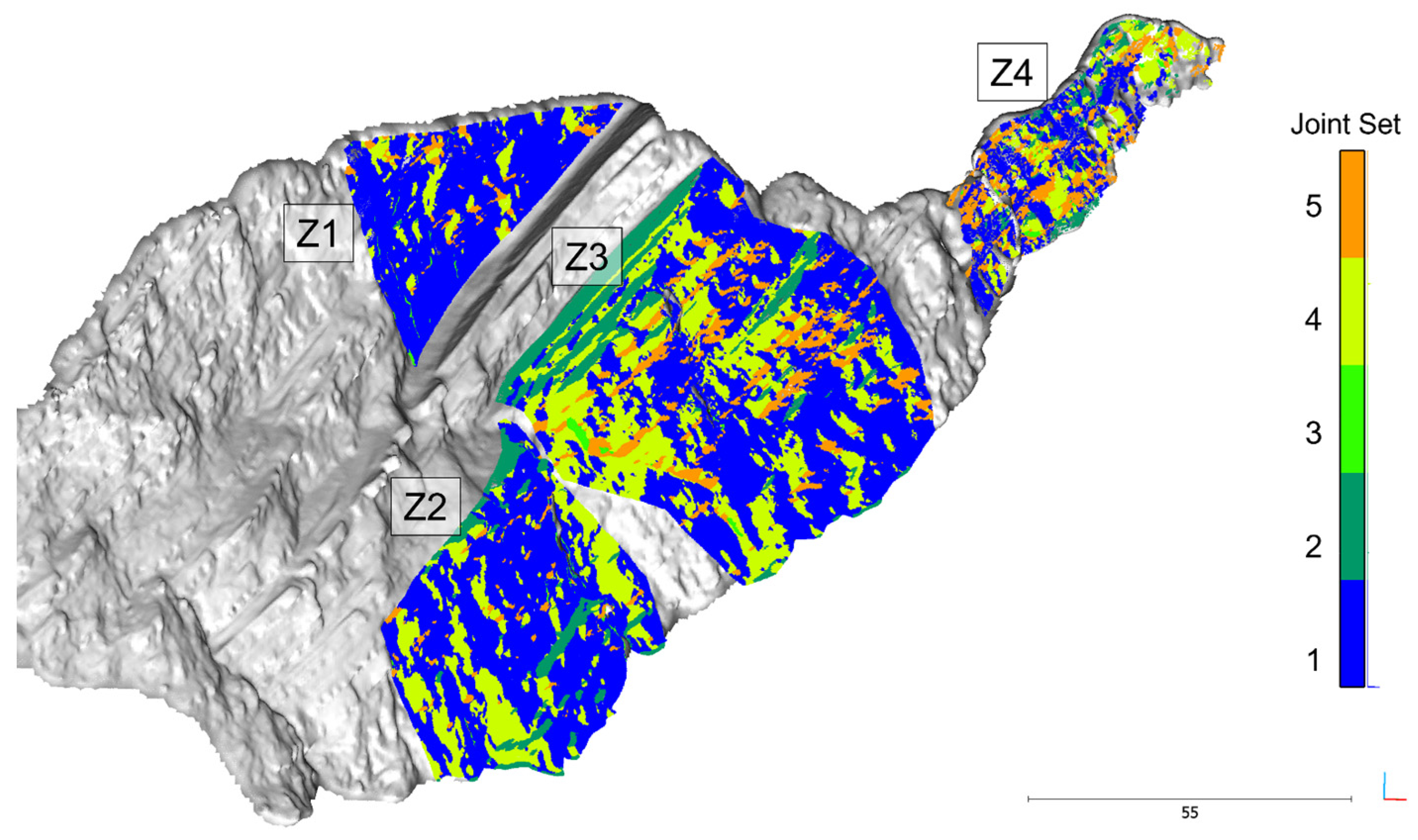
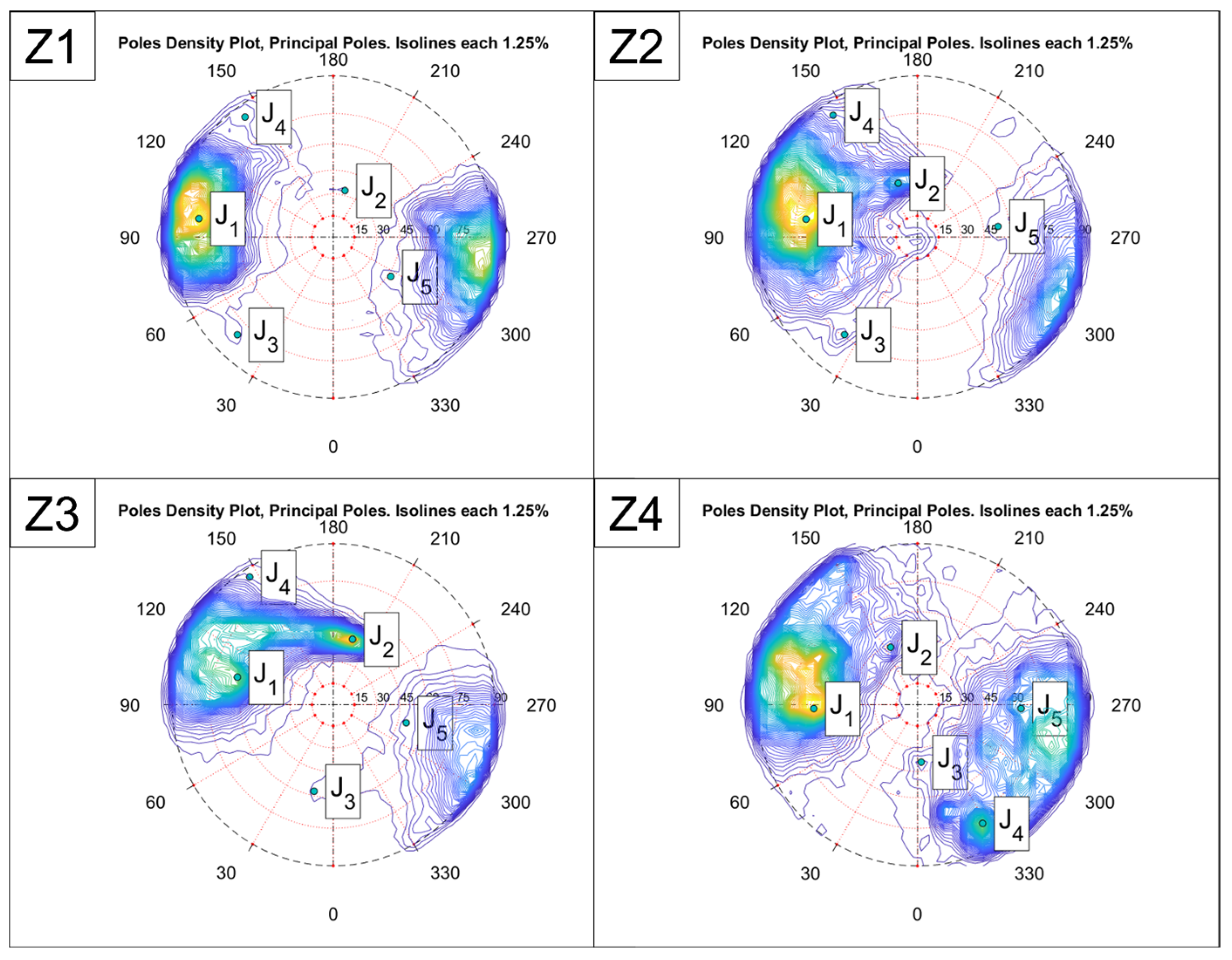
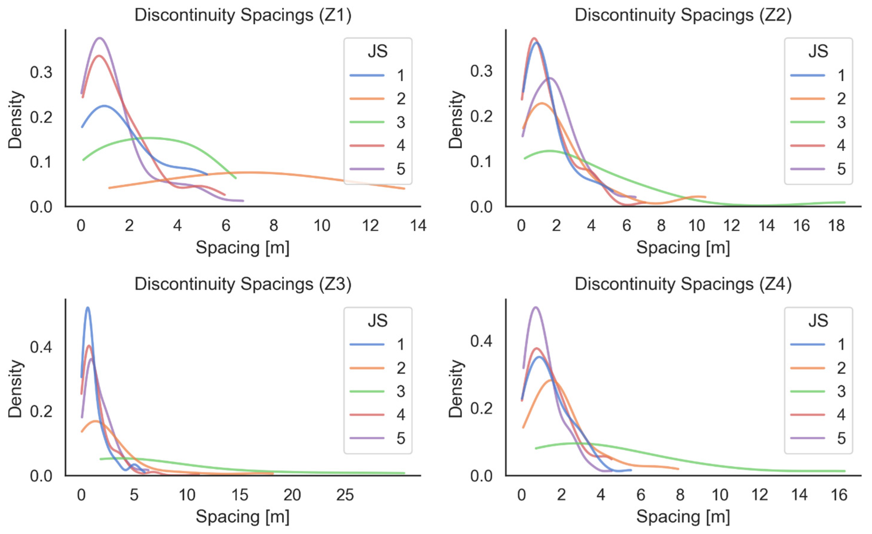
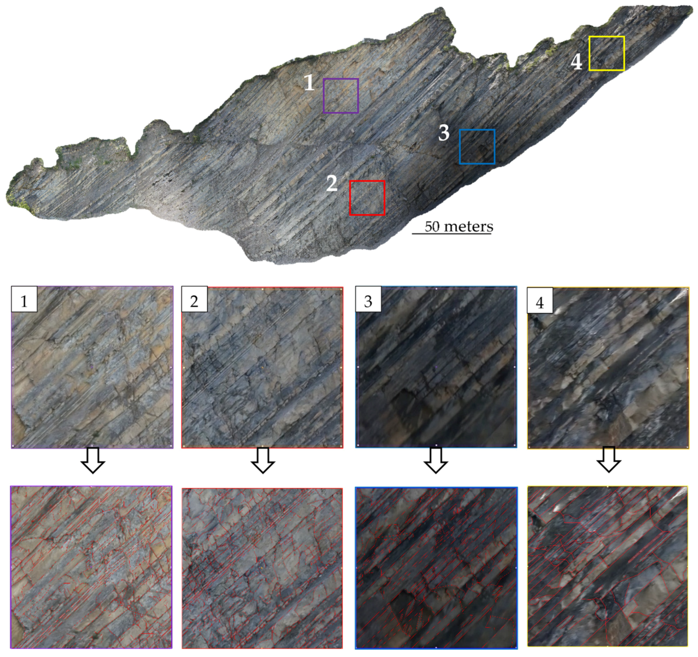
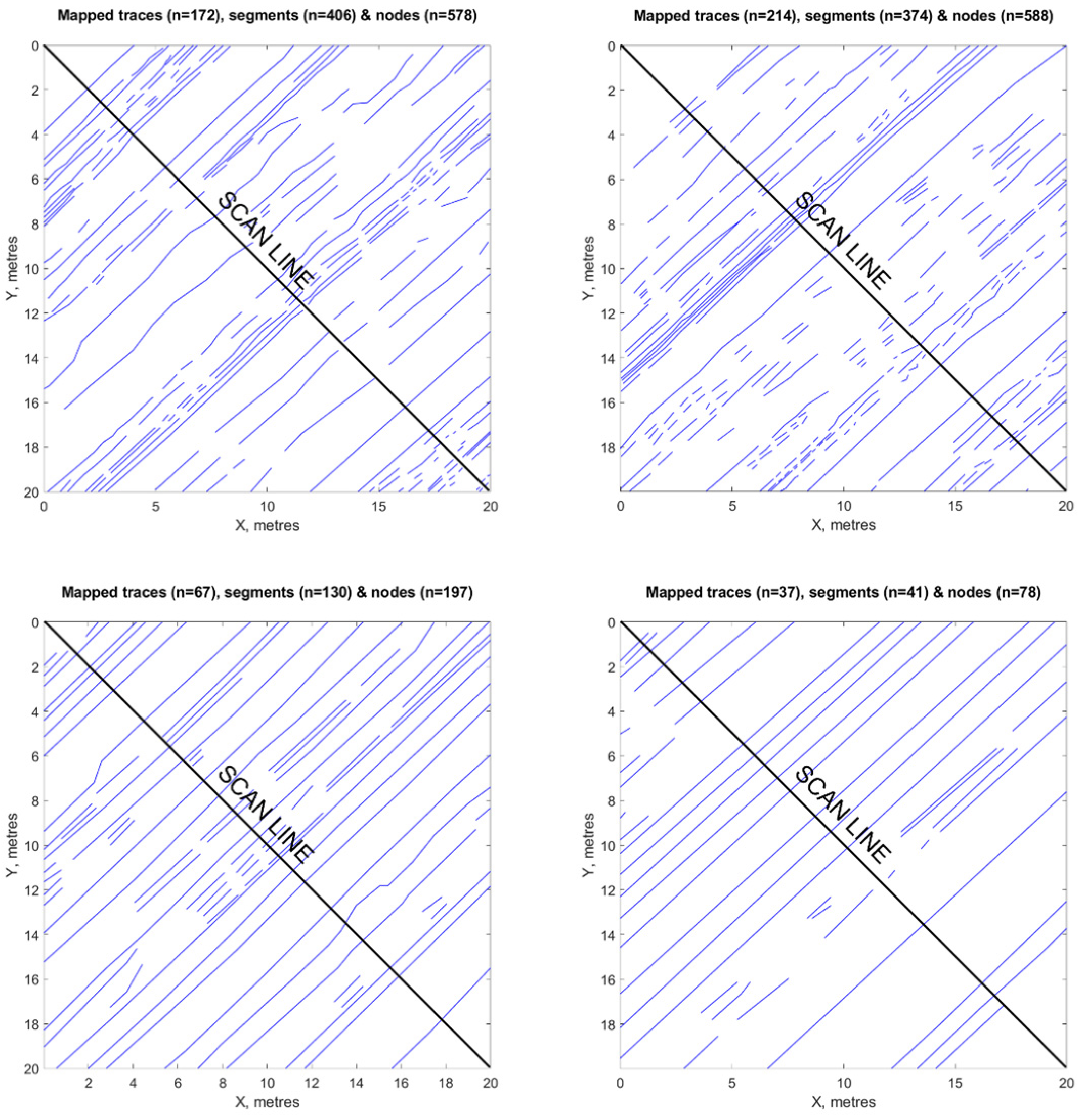
4.2. Geostructural Characterization
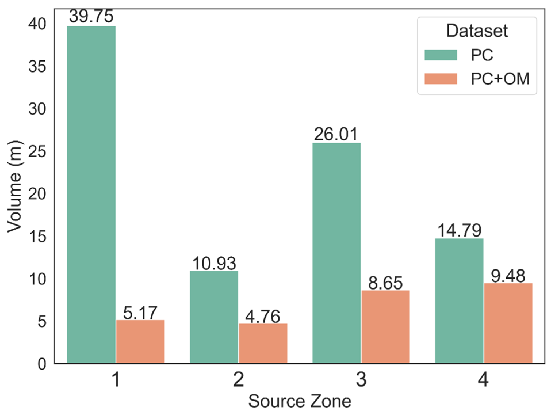
4.3. Three-Dimensional Rockfall Trajectory Analysis
5. Discussion
6. Conclusions
Author Contributions
Funding
Data Availability Statement
Acknowledgments
Conflicts of Interest
References
- Sarro, R.; Riquelme, A.; García-Davalillo, J.C.; Mateos, R.M.; Tomás, R.; Pastor, J.L.; Cano, M.; Herrera, G. Rockfall Simulation Based on UAV Photogrammetry Data Obtained during an Emergency Declaration: Application at a Cultural Heritage Site. Remote Sens. 2018, 10, 1923. [Google Scholar] [CrossRef]
- Francioni, M.; Antonaci, F.; Sciarra, N.; Robiati, C.; Coggan, J.; Stead, D.; Calamita, F. Application of Unmanned Aerial Vehicle Data and Discrete Fracture Network Models for Improved Rockfall Simulations. Remote Sens. 2020, 12, 2053. [Google Scholar] [CrossRef]
- Schilirò, L.; Robiati, C.; Smeraglia, L.; Vinci, F.; Iannace, A.; Parente, M.; Tavani, S. An Integrated Approach for the Reconstruction of Rockfall Scenarios from UAV and Satellite-Based Data in the Sorrento Peninsula (Southern Italy). Eng. Geol. 2022, 308, 106795. [Google Scholar] [CrossRef]
- Bonneau, D.A.; DiFrancesco, P.-M.; Hutchinson, D.J. A Method for Vegetation Extraction in Mountainous Terrain for Rockfall Simulation. Remote Sens. Environ. 2020, 251, 112098. [Google Scholar] [CrossRef]
- Rossi, M.; Sarro, R.; Reichenbach, P.; Mateos, R.M. Probabilistic Identification of Rockfall Source Areas at Regional Scale in El Hierro (Canary Islands, Spain). Geomorphology 2021, 381, 107661. [Google Scholar] [CrossRef]
- Guzzetti, F.; Reichenbach, P.; Ghigi, S. Rockfall Hazard and Risk Assessment along a Transportation Corridor in the Nera Valley, Central Italy. Environ. Manag. 2004, 34, 191–208. [Google Scholar] [CrossRef]
- Michoud, C.; Derron, M.-H.; Horton, P.; Jaboyedoff, M.; Baillifard, F.-J.; Loye, A.; Nicolet, P.; Pedrazzini, A.; Queyrel, A. Rockfall Hazard and Risk Assessments along Roads at a Regional Scale: Example in Swiss Alps. Nat. Hazards Earth Syst. Sci. 2012, 12, 615–629. [Google Scholar] [CrossRef]
- Scavia, C.; Barbero, M.; Castelli, M.; Marchelli, M.; Peila, D.; Torsello, G.; Vallero, G. Evaluating Rockfall Risk: Some Critical Aspects. Geosciences 2020, 10, 98. [Google Scholar] [CrossRef]
- Gili, J.A.; Ruiz-Carulla, R.; Matas, G.; Moya, J.; Prades, A.; Corominas, J.; Lantada, N.; Núñez-Andrés, M.A.; Buill, F.; Puig, C.; et al. Rockfalls: Analysis of the Block Fragmentation through Field Experiments. Landslides 2022, 19, 1009–1029. [Google Scholar] [CrossRef]
- Gallo, I.G.; Martínez-Corbella, M.; Sarro, R.; Iovine, G.; López-Vinielles, J.; Hérnandez, M.; Robustelli, G.; Mateos, R.M.; García-Davalillo, J.C. An Integration of UAV-Based Photogrammetry and 3D Modelling for Rockfall Hazard Assessment: The Cárcavos Case in 2018 (Spain). Remote Sens. 2021, 13, 3450. [Google Scholar] [CrossRef]
- Robiati, C.; Eyre, M.; Vanneschi, C.; Francioni, M.; Venn, A.; Coggan, J. Application of Remote Sensing Data for Evaluation of Rockfall Potential within a Quarry Slope. ISPRS Int. J. Geo. Inf. 2019, 8, 367. [Google Scholar] [CrossRef]
- Onsel, I.E.; Donati, D.; Stead, D.; Chang, O. Applications of Virtual and Mixed Reality in Rock Engineering. In Proceedings of the 52nd U.S. Rock Mechanics/Geomechanics Symposium, Seattle, Washington, 17–20 June 2018. [Google Scholar]
- Lato, M.J.; Diederichs, M.S.; Hutchinson, D.J.; Harrap, R. Evaluating Roadside Rockmasses for Rockfall Hazards Using LiDAR Data: Optimizing Data Collection and Processing Protocols. Nat. Hazards 2012, 60, 831–864. [Google Scholar] [CrossRef]
- Jaboyedoff, M.; Oppikofer, T.; Abellán, A.; Derron, M.-H.; Loye, A.; Metzger, R.; Pedrazzini, A. Use of LIDAR in Landslide Investigations: A Review. Nat. Hazards 2012, 61, 5–28. [Google Scholar] [CrossRef]
- Abellán, A.; Oppikofer, T.; Jaboyedoff, M.; Rosser, N.J.; Lim, M.; Lato, M.J. Terrestrial Laser Scanning of Rock Slope Instabilities. Earth Surf. Process. Landf. 2014, 39, 80–97. [Google Scholar] [CrossRef]
- Eltner, A.; Kaiser, A.; Castillo, C.; Rock, G.; Neugirg, F.; Abellán, A. Image-Based Surface Reconstruction in Geomorphometry – Merits, Limits and Developments. Earth Surf. Dyn. 2016, 4, 359–389. [Google Scholar] [CrossRef]
- Bonneau, D.; DiFrancesco, P.-M.; Hutchinson, D.J. Surface Reconstruction for Three-Dimensional Rockfall Volumetric Analysis. ISPRS Int. J. Geo. Inf. 2019, 8, 548. [Google Scholar] [CrossRef]
- Sarro, R.; María Mateos, R.; Reichenbach, P.; Aguilera, H.; Riquelme, A.; Hernández-Gutiérrez, L.E.; Martín, A.; Barra, A.; Solari, L.; Monserrat, O.; et al. Geotechnics for Rockfall Assessment in the Volcanic Island of Gran Canaria (Canary Islands, Spain). J. Maps 2020, 16, 605–613. [Google Scholar] [CrossRef]
- Francioni, M.; Stead, D.; Sciarra, N.; Calamita, F. A New Approach for Defining Slope Mass Rating in Heterogeneous Sedimentary Rocks Using a Combined Remote Sensing GIS Approach. Bull. Eng. Geol. Environ. 2019, 78, 4253–4274. [Google Scholar] [CrossRef]
- McKenzie, D. Active Tectonics of the Mediterranean Region. Geophys. J. Int. 1972, 30, 109–185. [Google Scholar] [CrossRef]
- Martelli, L.; Camassi, R.; Catanzariti, R.; Fornaciari, L.; Spadafora, E. Explanatory Notes of the Geological Map of Italy, Scale 1:50,000, Sheet 265 “Bagno Di Romagna”; APAT and Geological Survey of Italy: Rome, Italy, 2002. [Google Scholar]
- Ricci Lucchi, F. The Miocene Marnoso-Arenacea Turbidites, Romagna and Umbria Apennines. Excursion N 7, Excursion Guidebook. In Proceedings of the 2nd International Association of Sedimentologists Regional Meeting, Bologna, Italy, 13–15 April 1981. [Google Scholar]
- Benini, A.; Farabegoli, E.; Martelli, L.; Severi, P. Stratigrafia e Paleogeografia Del Gruppo Di S. Sofia (Alto Appennino Forlivese). Mem. Descr. Della Carta Geol. d’Ital. 1992, 46, 231–243. [Google Scholar]
- Mutti, E.; Bernoulli, D.; Lucchi, F.R.; Tinterri, R. Turbidites and Turbidity Currents from Alpine ‘Flysch’ to the Exploration of Continental Margins. Sedimentology 2009, 56, 267–318. [Google Scholar] [CrossRef]
- Esposito, C.; Di Luzio, E.; Baleani, M.; Troiani, F.; Seta, M.D.; Bozzano, F.; Mazzanti, P. Fold architecture predisposing deep-seated gravitational slope deformations within a flysch sequence in the northern apennines (Italy). Geomorphology 2021, 380, 107629. [Google Scholar] [CrossRef]
- Bortolotti, V. Guide Geologiche Regionali. Appennino Tosco-Emiliano; BE-MA: Milano, Italy, 1992. [Google Scholar]
- Benini, A.; Biavati, G.; Generali, M.; Pizziolo, M. The Poggio Baldi Landslide (High Bidente Valley): Event and Post-Event Analysis and Geological Characterization. In Proceedings of the 7th EUREGEO–European Congress on Regional GEOscientific Cartography and Information Systems, Bologna, Italy, 12–15 June 2012; pp. 64–65. [Google Scholar]
- Mazzanti, P.; Bozzano, F.; Brunetti, A.; Caporossi, P.; Esposito, C.; Mugnozza, G.S. Experimental Landslide Monitoring Site of Poggio Baldi Landslide (Santa Sofia, N-Apennine, Italy). In Proceedings of the Advancing Culture of Living with Landslides; Mikoš, M., Arbanas, Ž., Yin, Y., Sassa, K., Eds.; Springer International Publishing: Cham, Switzerland, 2017; pp. 259–266. [Google Scholar]
- Varnes, D.J. Slope Movement Types and Processes. Spec. Rep. 1978, 176, 11–33. [Google Scholar]
- Mazzanti, P.; Caporossi, P.; Brunetti, A.; Mohammadi, F.I.; Bozzano, F. Short-Term Geomorphological Evolution of the Poggio Baldi Landslide Upper Scarp via 3D Change Detection. Landslides 2021, 18, 2367–2381. [Google Scholar] [CrossRef]
- Romeo, S.; Cosentino, A.; Giani, F.; Mastrantoni, G.; Mazzanti, P. Combining Ground Based Remote Sensing Tools for Rockfalls Assessment and Monitoring: The Poggio Baldi Landslide Natural Laboratory. Sensors 2021, 21, 2632. [Google Scholar] [CrossRef] [PubMed]
- Girardeau-Montaut, D. Détection de Changement Sur Des Données Géométriques Tridimensionnelles. Ph.D. Thesis, Télécom ParisTech, Paris, France, 2006. [Google Scholar]
- Spetsakis, M.E.; Aloimonos, J. (Yiannis) Structure from Motion Using Line Correspondences. Int. J. Comput. Vis. 1990, 4, 171–183. [Google Scholar] [CrossRef]
- Boufama, B.; Mohr, R.; Veillon, F. Euclidean Constraints for Uncalibrated Reconstruction. In Proceedings of the 1993 (4th) International Conference on Computer Vision, Berlin, Germany, 11–14 May 1993; pp. 466–470. [Google Scholar]
- Szeliski, R.; Kang, S.B. Recovering 3D Shape and Motion from Image Streams Using Nonlinear Least Squares. J. Vis. Commun. Image Represent. 1994, 5, 10–28. [Google Scholar] [CrossRef]
- Seitz, S.M.; Curless, B.; Diebel, J.; Scharstein, D.; Szeliski, R. A Comparison and Evaluation of Multi-View Stereo Reconstruction Algorithms. In Proceedings of the 2006 IEEE Computer Society Conference on Computer Vision and Pattern Recognition (CVPR’06), New York, NY, USA, 17–22 June 2006; Volume 1, pp. 519–528. [Google Scholar]
- James, M.R.; Robson, S. Straightforward Reconstruction of 3D Surfaces and Topography with a Camera: Accuracy and Geoscience Application. J. Geophys. Res. Earth Surf. 2012, 117, F03017. [Google Scholar] [CrossRef]
- Luhmann, T.; Robson, S.; Kyle, S.; Boehm, J. Close-Range Photogrammetry and 3D Imaging; De Gruyter: Berlin, Germany, 2019; ISBN 978-3-11-060725-3. [Google Scholar]
- Carrivick, J.L.; Smith, M.W.; Quincey, D.J. Structure from Motion in the Geosciences; John and Wiley and Sons: Hoboken, NJ, USA, 2016; ISBN 978-1-118-89583-2. [Google Scholar]
- Snavely, N.; Seitz, S.M.; Szeliski, R. Modeling the World from Internet Photo Collections. Int. J. Comput. Vis. 2008, 80, 189–210. [Google Scholar] [CrossRef]
- Arya, S.; Mount, D.M.; Netanyahu, N.S.; Silverman, R.; Wu, A.Y. An Optimal Algorithm for Approximate Nearest Neighbor Searching Fixed Dimensions. J. ACM 1998, 45, 891–923. [Google Scholar] [CrossRef]
- Fischler, M.A.; Bolles, R.C. Random Sample Consensus: A Paradigm for Model Fitting with Applications to Image Analysis and Automated Cartography. Commun. ACM 1981, 24, 381–395. [Google Scholar] [CrossRef]
- Lague, D.; Brodu, N.; Leroux, J. Accurate 3D Comparison of Complex Topography with Terrestrial Laser Scanner: Application to the Rangitikei Canyon (N-Z). ISPRS J. Photogramm. Remote Sens. 2013, 82, 10–26. [Google Scholar] [CrossRef]
- Stumpf, A.; Malet, J.-P.; Allemand, P.; Pierrot-Deseilligny, M.; Skupinski, G. Ground-Based Multi-View Photogrammetry for the Monitoring of Landslide Deformation and Erosion. Geomorphology 2015, 231, 130–145. [Google Scholar] [CrossRef]
- Riquelme, A.J.; Abellán, A.; Tomás, R.; Jaboyedoff, M. A New Approach for Semi-Automatic Rock Mass Joints Recognition from 3D Point Clouds. Comput. Geosci. 2014, 68, 38–52. [Google Scholar] [CrossRef]
- Riquelme, A.; Cano, M.; Tomás, R.; Abellán, A. Identification of Rock Slope Discontinuity Sets from Laser Scanner and Photogrammetric Point Clouds: A Comparative Analysis. Procedia Eng. 2017, 191, 838–845. [Google Scholar] [CrossRef]
- Friedman, J.H. A Recursive Partitioning Decision Rule for Nonparametric Classification. IEEE Trans. Comput. 1977, 26, 404–408. [Google Scholar] [CrossRef]
- Botev, Z.I.; Grotowski, J.F.; Kroese, D.P. Kernel Density Estimation via Diffusion. Ann. Stat. 2010, 38, 2916–2957. [Google Scholar] [CrossRef]
- Ester, M.; Kriegel, H.-P.; Sander, J.; Xu, X. A Density-Based Algorithm for Discovering Clusters in Large Spatial Databases with Noise. In Proceedings of the Second International Conference on Knowledge Discovery and Data Mining; AAAI Press: Portland, Oregon, 1996; pp. 226–231. [Google Scholar]
- Farmakis, I.; Hutchinson, D.J. Semi-Automated Discontinuity Orientation Extraction in Complex Rock Masses Using Single-Scan LiDAR Data. Geophys. Res. Abstr. 2019, 21, 1. [Google Scholar]
- Farmakis, I.; Marinos, V.; Papathanassiou, G.; Karantanellis, E. Automated 3D Jointed Rock Mass Structural Analysis and Characterization Using LiDAR Terrestrial Laser Scanner for Rockfall Susceptibility Assessment: Perissa Area Case (Santorini). Geotech. Geol. Eng. 2020, 38, 3007–3024. [Google Scholar] [CrossRef]
- Riquelme, A.J.; Abellán, A.; Tomás, R. Discontinuity Spacing Analysis in Rock Masses Using 3D Point Clouds. Eng. Geol. 2015, 195, 185–195. [Google Scholar] [CrossRef]
- Palmstrom, A. Measurements of and Correlations between Block Size and Rock Quality Designation (RQD). Tunn. Undergr. Space Technol. 2005, 20, 362–377. [Google Scholar] [CrossRef]
- Healy, D.; Rizzo, R.E.; Cornwell, D.G.; Farrell, N.J.C.; Watkins, H.; Timms, N.E.; Gomez-Rivas, E.; Smith, M. FracPaQ: A MATLABTM Toolbox for the Quantification of Fracture Patterns. J. Struct. Geol. 2017, 95, 1–16. [Google Scholar] [CrossRef]
- Hantz, D.; Corominas, J.; Crosta, G.B.; Jaboyedoff, M. Definitions and Concepts for Quantitative Rockfall Hazard and Risk Analysis. Geosciences 2021, 11, 158. [Google Scholar] [CrossRef]
- Ferrari, F.; Giacomini, A.; Thoeni, K. Qualitative Rockfall Hazard Assessment: A Comprehensive Review of Current Practices. Rock Mech. Rock Eng. 2016, 49, 2865–2922. [Google Scholar] [CrossRef]
- Volkwein, A.; Schellenberg, K.; Labiouse, V.; Agliardi, F.; Berger, F.; Bourrier, F.; Dorren, L.K.A.; Gerber, W.; Jaboyedoff, M. Rockfall Characterisation and Structural Protection—A Review. Nat. Hazards Earth Syst. Sci. 2011, 11, 2617–2651. [Google Scholar] [CrossRef]
- Noël, F.; Cloutier, C.; Jaboyedoff, M.; Locat, J. Impact-Detection Algorithm That Uses Point Clouds as Topographic Inputs for 3D Rockfall Simulations. Geosciences 2021, 11, 188. [Google Scholar] [CrossRef]
- Dorren, L.K.A. A Review of Rockfall Mechanics and Modelling Approaches. Prog. Phys. Geogr. Earth Environ. 2003, 27, 69–87. [Google Scholar] [CrossRef]
- Ritchie, A.M. Evaluation of Rockfall and Its Control. Highw. Res. Rec. 1963, 17, 13–28. [Google Scholar]
- Mitchell, A.; Hungr, O. Theory and Calibration of the Pierre 2 Stochastic Rock Fall Dynamics Simulation Program. Can. Geotech. J. 2017, 54, 18–30. [Google Scholar] [CrossRef]
- Asteriou, P.; Tsiambaos, G. Effect of Impact Velocity, Block Mass and Hardness on the Coefficients of Restitution for Rockfall Analysis. Int. J. Rock Mech. Min. Sci. 2018, 106, 41–50. [Google Scholar] [CrossRef]
- Dorren, L.K.A. Rockyfor3D (v5. 2) Revealed–Transparent Description of the Complete 3D Rockfall Model; Int ecorisQ Association: Geneva, Switzerland, 2016; p. 32. [Google Scholar]
- Vanneschi, C.; Rindinella, A.; Salvini, R. Hazard Assessment of Rocky Slopes: An Integrated Photogrammetry–GIS Approach Including Fracture Density and Probability of Failure Data. Remote Sens. 2022, 14, 1438. [Google Scholar] [CrossRef]
- Moos, C.; Bontognali, Z.; Dorren, L.; Jaboyedoff, M.; Hantz, D. Estimating Rockfall and Block Volume Scenarios Based on a Straightforward Rockfall Frequency Model. Eng. Geol. 2022, 309, 106828. [Google Scholar] [CrossRef]


| Source Sector | Process | Estimated Surface (m2) | Estimated Volume (m3) |
|---|---|---|---|
| 1 | Rockfalls | 1441 | 620 |
| 2 | Rockfalls | 1805 | 475 |
| 3 | Rockfalls | 2795 | 817 |
| 4 | Rockfalls | 1479 | 1196 |
| Toe | Debris accumulation | 4572 | 5160 |
| Joint Set | Type of Discontinuity | Z1 | Z2 | Z3 | Z4 | ||||
|---|---|---|---|---|---|---|---|---|---|
| Dip-Dir | Dip-Angle | Dip-Dir | Dip-Angle | Dip-Dir | Dip-Angle | Dip-Dir | Dip-Angle | ||
| 1 | Slope Face | 98 | 80 | 99 | 70 | 105 | 64 | 88 | 65 |
| 2 | Bedding | 194 | 33 | 160 | 39 | 196 | 46 | 155 | 43 |
| 3 | Minor Joint | 44 | 80 | 37 | 74 | 12 | 57 | 356 | 39 |
| 4 | Minor Joint | 143 | 85 | 145 | 85 | 146 | 87 | 331 | 80 |
| 5 | Minor Joint | 304 | 47 | 262 | 54 | 284 | 50 | 272 | 65 |
| Joint Set | Z1 | Z2 | Z3 | Z4 |
|---|---|---|---|---|
| J1 | 1.902 | 1.449 | 1.197 | 1.443 |
| J2 | 7.223 | 2.227 | 2.767 | 2.151 |
| J2-OM | 0.940 | 0.970 | 0.920 | 1.380 |
| J3 | 2.894 | 3.384 | 7.858 | 4.764 |
| J4 | 1.569 | 1.536 | 1.450 | 1.455 |
| J5 | 1.458 | 1.975 | 1.715 | 1.146 |
| Terrain Description | RF3D Soil Type | rg70 (m) | rg20 (m) | rg10 (m) | Rn Avg | Rn Range |
|---|---|---|---|---|---|---|
| Landslide scarp | 6 | 0 | 0.1 | 0.5 | 0.53 | 0.48–0.58 |
| Thinly covered bedrock | 5 | 0.1 | 0.2 | 0.3 | 0.43 | 0.39–0.47 |
| Marls and claystone | 3 | 0 | 0.1 | 0.3 | 0.33 | 0.30–0.36 |
| Talus slope | 3 | 0.25 | 0.5 | 0.9 | 0.33 | 0.30–0.36 |
| Flat surface | 3 | 0 | 0.1 | 0.5 | 0.33 | 0.30–0.36 |
| Engineered slope | 2 | 0 | 0.1 | 0.2 | 0.28 | 0.25–0.31 |
| Vegetation | 1 | 0.3 | 0.4 | 0.6 | 0.23 | 0.21–0.25 |
| Rock barrier | 1 | 0 | 0 | 100 | 0.23 | 0.21–0.25 |
| Sector | Source Pixels | Total Trajectories | PC + OM Block Volume (m3) | PC Block Volume (m3) |
|---|---|---|---|---|
| 1 | 48 | 48 × 104 | 5.17 | 39.75 |
| 2 | 22 | 22 × 104 | 4.76 | 10.93 |
| 3 | 15 | 15 × 104 | 8.65 | 26.01 |
| 4 | 84 | 84 × 104 | 9.48 | 14.79 |
Disclaimer/Publisher’s Note: The statements, opinions and data contained in all publications are solely those of the individual author(s) and contributor(s) and not of MDPI and/or the editor(s). MDPI and/or the editor(s) disclaim responsibility for any injury to people or property resulting from any ideas, methods, instructions or products referred to in the content. |
© 2023 by the authors. Licensee MDPI, Basel, Switzerland. This article is an open access article distributed under the terms and conditions of the Creative Commons Attribution (CC BY) license (https://creativecommons.org/licenses/by/4.0/).
Share and Cite
Robiati, C.; Mastrantoni, G.; Francioni, M.; Eyre, M.; Coggan, J.; Mazzanti, P. Contribution of High-Resolution Virtual Outcrop Models for the Definition of Rockfall Activity and Associated Hazard Modelling. Land 2023, 12, 191. https://doi.org/10.3390/land12010191
Robiati C, Mastrantoni G, Francioni M, Eyre M, Coggan J, Mazzanti P. Contribution of High-Resolution Virtual Outcrop Models for the Definition of Rockfall Activity and Associated Hazard Modelling. Land. 2023; 12(1):191. https://doi.org/10.3390/land12010191
Chicago/Turabian StyleRobiati, Carlo, Giandomenico Mastrantoni, Mirko Francioni, Matthew Eyre, John Coggan, and Paolo Mazzanti. 2023. "Contribution of High-Resolution Virtual Outcrop Models for the Definition of Rockfall Activity and Associated Hazard Modelling" Land 12, no. 1: 191. https://doi.org/10.3390/land12010191
APA StyleRobiati, C., Mastrantoni, G., Francioni, M., Eyre, M., Coggan, J., & Mazzanti, P. (2023). Contribution of High-Resolution Virtual Outcrop Models for the Definition of Rockfall Activity and Associated Hazard Modelling. Land, 12(1), 191. https://doi.org/10.3390/land12010191