High Resolution Land Cover Integrating Copernicus Products: A 2012–2020 Map of Italy

Abstract

The study involved an in-depth analysis of the main land cover and land use data available nationwide for the Italian territory, in order to produce a reliable cartography for the evaluation of ecosystem services. In detail, data from the land monitoring service of the Copernicus Programme were taken into consideration, while at national level the National Land Consumption Map and some regional land cover and land use maps were analysed. The classification systems were standardized with respect to the European specifications of the EAGLE Group and the data were integrated to produce a land cover map in raster format with a spatial resolution of 10 m. The map was validated and compared with the CORINE Land Cover, showing a significant geometric and thematic improvement, useful for a more detailed and reliable evaluation of ecosystem services. In detail, the map was used to estimate the variation in carbon storage capacity in Italy for the period 2012–2020, linked to the increase in land consumption

1. Introduction

Territory is a source of resources such as food, biomass and raw materials and provides essential ecosystem services that support production functions, regulate natural cycles, provide cultural and spiritual benefits [1].

The European Environment Agency introduced the concept of “land system”, which defines the territory as a set of terrestrial components that includes all the processes and activities related to its anthropic use [2,3]. This concept considers the territory as an integrated system [4] that combines everything related to land use and land cover. The study of land cover and land use is essential to understand the causes and effects of human-determined changes [5], seeing as now changes and transformations that occur within the land system lead to consequences for the well-being of humans and the environment at the local, regional and global levels.

1.1. Estimation and Monitoring of Ecosystem Services

The management of territory is fundamental, since its transformation alters the environmental processes and related ecosystem services [6], which are the benefits that humans obtain directly or indirectly from terrestrial ecosystems [7].

Since 2005, the concept of ecosystem services has been placed on the political agenda [8,9,10] thanks also to the Millennium Ecosystem Assessment (MEA). The MEA is an international research project launched in 2001 with the aim of evaluating the consequences of ecosystem changes on human well-being and establishing actions to improve the conservation and sustainable use of ecosystems and their contribution to health.

The Millennium Ecosystem Assessment [11] provides a classification of ecosystem services which consist of four groups:

–

Provisioning services, which provide products obtained from ecosystems, such as food, raw materials and water.

–

Regulating services, i.e., the benefits provided through ecosystem processes, such as carbon storage, erosion control.

–

Cultural services, which represent the nonmaterial benefits that people obtain through spiritual enrichment, cognitive development and aesthetic experience.

–

Supporting services, which constitute a “transversal” category that supports the production of other services, providing living space for plants and animals or maintaining genetic diversity. They differ from other categories since their impact on people is indirect or is visible after a very long period.

The Economics of Ecosystems and Biodiversity [12] provides a classification aligned with MEA, while the Common International Classification of Ecosystem Services (CICES) excludes “support services” and renames the category of “regulation services” as “regulation and maintenance services”, including habitat maintenance [13,14].

In 1997, Costanza [7] published one of the first assessments of ecosystem services, which was then updated in 2014 [15]. Other application examples for more limited areas are readily available in the scientific literature: assessment on pollination can be found both from a biophysical [16,17] and economic [18,19,20] point of view. The United Kingdom was among the first European country to draw up a complete official report in line with the Millennium Ecosystem Assessment [21]. Rabe et al. [22] developed a network of national indicators on ecosystem services in Germany using CORINE Land Cover data for the analysis of nine ecosystem services divided into three classification categories (according to CICES). Spain published an official report in 2016 [23] related to twelve ecosystem services. Outside the European context, there are applications on a national scale in China [24], South Africa [25] and South Korea [26].

Soil has fundamental functions for nature and humankind and is the source of many ecosystem services [27,28,29]:

–

Fertility: the nutrient cycle ensures fertility in the soil and, at the same time, the release of nutrients necessary for plant growth;

–

Filter and reserve: the soil can act as a filter against pollutants and can store large quantities of water, useful for plants and for the mitigation of floods;

–

Structural: soils represent the support for plants, animals and infrastructures;

–

Climate regulation: the soil, in addition to being the largest carbon sink, regulates the emission of important greenhouse gases (N₂O and CH₄);

–

Conservation of biodiversity: soils are an immense reservoir of biodiversity. They represent the habitat for thousands of species capable of preventing the action of parasites or facilitating waste disposal;

–

Resource: soils can be an important source of supply of raw materials.

All soils perform their functions at the same time (food production, water purification, carbon sequestration, etc.) in a different way according to land use and pedogenetic characteristics. For example, the rate of carbon sequestration and water purification is higher in a natural area than in an agricultural one, which however has greater production capacity.

Carbon sequestration and storage is an important regulatory service linked to the attitude of ecosystems to fix greenhouse gases. This service contributes to climate regulation and is fundamental in defining adaptation strategies to climate change [30,31]. The capacity to store carbon depends, among other things, on land use and cover and on the climate [32]. Land use, land use change and forestry (LULUCF) activities can act as sources of emissions or store carbon by acting as sinks. In particular, natural and seminatural forest ecosystems have the highest carbon sequestration potential. Once natural land is urbanized or degraded, it loses its ability to retain carbon which, as a result, is emitted into the atmosphere [33]. Urban expansion, land consumption, deforestation and forest degradation limit the ability of natural areas to store carbon and have contributed to these emissions by releasing carbon stored in forests, vegetation and soil [6,34,35].

1.2. Land Monitoring

Land cover and land use are strongly related and for many applications both information categories are required [36]. To meet different monitoring needs, data with different characteristics from a spatial, temporal and thematic point of view were introduced.

In this respect, different initiatives have been developed. The purpose of the Copernicus program is to collect information on the earth’s surface and organize it according to criteria that allow to compare different data, to exchange data between EU countries and to increase the number of users. The Copernicus Land Monitoring Service (CLMS) allows researchers to obtain geographic information on soils and on numerous variables related to them (such as the state of the vegetation or the water cycle), supporting applications in a wide variety of sectors, such as territorial planning, management of water resources and forests, agriculture and food security. CORINE Land Cover is one of the main products belonging to CLMS. It has guaranteed information for the whole European territory since 1990, with 44 land cover and land use classes and geometric detail of 25 hectares.

Recently, data with higher spatial and thematic details have been introduced in the context of the CLMS Local Component. It aims at providing detailed information on critical areas from an environmental point of view, which require specific and detailed monitoring. Currently, this Copernicus component offers land cover and land use maps in vector format, with high spatial resolution and a 6-year update frequency for four categories of areas. Urban Atlas refers to the CLC classification system, describing with higher detail the land cover and land use characteristics of urban areas, while Riparian Zone and Natura 2000 use the ecosystem types defined in the Mapping Assessment of Ecosystems and their Services (MAES) [37], which are based on the CLC classes too.

These aforementioned data adopt classification systems based on different combinations of land cover and land use classes that are difficult to compare and integrate with those of other data. In order to coordinate data flows from a thematic point of view, the EAGLE group (EIONET Action Group on Land monitoring in Europe) was created. It aims at defining a conceptual methodology to describe land cover and land use information in a consistent data model. EAGLE is not a classification system but a tool to describe classes of a given classification system by tracing them to the segments related to the three categories. This allows to better understand the characteristics, the overlaps and the possible conversions between different classification systems and provides a basis to define new ones. The EAGLE model aims at separating the land cover and land use components through data modelling systems applicable at different scales and in different contexts, while maintaining compatibility with existing databases.

The EAGLE data model is based on the definition of three blocks, called “categories”:

• Land cover components (LCC), which refer to the definition of "land cover" provided by the INSPIRE directive 2007/2/CE. The LCCs are mutually exclusive and exhaustive and can be used as a modelling element to semantically describe a class definition or to map landscape;
• Land use attributes (LUA), that follow in principle the Hierarchical INSPIRE Land Use Classification System (HILUCS), with some changes to fit the purpose of the EAGLE concept. The LUA are attached to the land cover unit;
• Landscape characteristics (CH), which describe further details of the land cover components. The first level distinguishes “land management”, “spatial pattern”, “crop type", “mining product type”, “ecosystem types”, “height zone”, “(bio-)physical characteristics”, “general parameters”, “status” and “temporal” parameters. This enhances the integration between national activities and European land monitoring initiatives encouraging a bottom-up approach in data production.

The problem of interoperability and non-homogeneity between data is also evident at a national level. The National Land Consumption Map offers national coverage, with annual update and EAGLE compliant classification system, while most of the data available at the regional level are inconsistent, not updated and difficult to relate to each other.

Despite the large amount and variety of land cover and land use data available at national and European level, currently CLC is the only product capable of supporting an assessment of ecosystem services on a national scale [38], since it guarantees the mapping of the entire national territory and has a thematic detail suitable for the purpose. However, the low spatial resolution and the presence of mixed classes reduce the reliability of the assessments based on them.

In this sense, the first objective of this research concerns the development of a methodology that makes the main Copernicus and national land cover and land use data comparable and integrable, in order to obtain a product with national coverage that allows to overcome the limits of the CLC in terms of classification system and geometric detail.

Furthermore, the activity refers to an EAGLE compliant classification system with a thematic detail useful for conducting an assessment of ecosystem services, with particular reference to the variation of carbon stocks. This change was assessed with respect to theincrease in land consumption between 2012 and 2020.

2. Materials and Methods

2.1. Overview

The methodology presented in this study integrates Copernicus and national data for the production of a land cover map capable of supporting the ecosystem services assessment. Data were reclassified according to an EAGLE compliant classification system and merged into a 10 m resolution land cover map of Italy. The map was used to assess the loss of carbon storage capacity for the period 2012–2020, associated with land consumption (Figure 1).

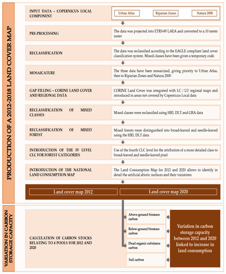
Figure 1. Workflow of the methodology for the production of the land cover map and evaluation of ecosystem services. The mosaic between Urban Atlas, Riparian Zones, and Natura 2000 was created (projected and rasterized at 10 m), then supplemented with the regional maps and CORINE Land Cover in the areas not covered by these three data. The distinction of forest categories and mixed classes was based on HRLs, while the National Land Consumption Map for 2012 and 2020 made it possible to identify artificial abiotic surfaces and their variation. The map allowed the calculation of three of the four pools considered for the estimation of the variation in carbon storage capacity.

2.2. Study Area

The analysis was carried out for the entire Italian territory (Figure 2), which covers 301,338 km². The country is composed mainly of hills (41.0%) and mountains (35.0%), while the remaining 23.0% of the territory is covered by plains. To the north is the mountain range of the Alps, which exceeds 4,000 m in altitude. In this area, the alpine climate prevails, with high rainfall with a maximum of 2,500–3,500 mm. In the peninsular area there is the Apennine mountain range, reaching its highest peak in Abruzzo with Gran Sasso (2,912 m) and characterized by a continental climate. The coastal area has a Mediterranean climate, with average annual rainfall that reaches a minimum of 500 mm in Apulia and Molise.

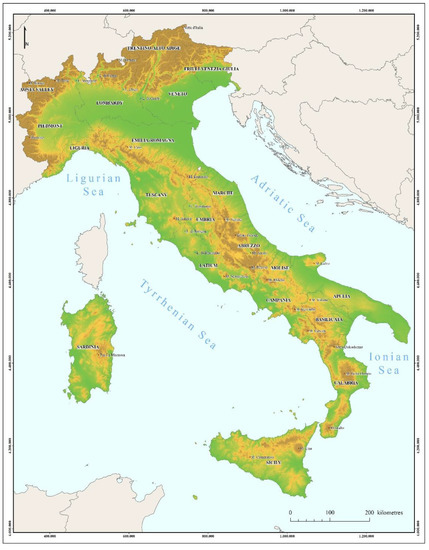
Figure 2. Study area—Italy.

Land cover is characterized by forest in mountain areas, with conifer concentration in alpine areas. Crops and most of the urbanized areas are concentrated in the plains and along the coast.

2.3. Land Cover Classification System

The activities described in this paper refers to a sixteen-class classification system. The classes are defined in accordance with the EAGLE group specifications [39,40,41] and are organized into five levels (Table 1).

Table 1. Land cover classification system.

Land Cover
I Level		II Level		III Level		IV Level		V Level
1	Abiotic Non-vegetated surfaces	11	Artificial abiotic
		12	Natural abiotic	121	Consolidated (bare rocks, cliffs)
				122	Unconsolidated (beaches, dunes, sands)
2	Biotic vegetated surfaces	21	Woody vegetation	211	Trees	2111	Broad-leaved
						2112	Needle-leaved
						2113	Permanent crops	21131	Orchards
								21132	Olive groves
								21133	Wood plantations
				212	Shrubs	2121	Vineyards
						2122	Shrubland
		22	Herbaceous vegetation	221	Periodically	2211	Pastures
						2212	Arable land
				222	Permanent
3	Water surfaces	31	Water bodies
		32	Permanent snow and ice
4	Wetlands

The classification system is based on previous activities of the working group [41] and improved to maintain the thematic detail offered by the Copernicus and national input data. The first three classes coincide up to the third level of detail with Eagle concept land cover components. Wetland class and the fourth and fifth classification levels are based on EAGLE characteristics (LCH) definitions.

• Abiotic non-vegetated: The class includes any unvegetated surfaces. At the second classification level, the class is subdivided between man-made artificial structures (artificial abiotic surfaces) and natural material surfaces (natural abiotic surfaces).

Artificial abiotic surfaces include impervious surfaces and reversible land consumption, according to the definition of ISPRA National Land Consumption Map [42]. Reversible land consumption indicates areas where the natural cover has been removed or replaced due to anthropogenic interventions, such as soil compaction or excavation, forming a non-impermeable and undeveloped surface. The main difference from the EAGLE model is the inclusion of quarries and extraction sites in this class, as detailed by De Fioravante et al. [41]. Natural abiotic surfaces are any kind of material that remains in its natural consistence or form, either with or without anthropogenic influence. The latter class presents a third-level distinction between consolidated unvegetated natural surfaces (bare rocks, cliffs) and unconsolidated unvegetated natural surfaces (beaches, dunes, sands).

2.

Biotic vegetated: The class includes any vegetated surfaces, with or without anthropogenic influence. At the second classification level, woody and herbaceous vegetation are distinguished.

The third classification level of woody vegetation divides trees and shrubs. Trees are then classified at the fourth level among broad-leaved, needle-leaved and permanent crops. Broad-leaved and needle-leaved have a fifth level based on CORINE Land Cover, while permanent crops distinguish olive groves, orchards and woody plantation. Shrubs are distinguished on the fourth level in vineyards and natural areas.

Herbaceous vegetation is divided into periodic and permanent. The periodic herbaceous class corresponds to the managed areas, subdivided at the fourth level into pastures and arable land, while the natural herbaceous is related to natural unmanaged grassland.

3.

Water surfaces: The class includes natural or artificial solid and liquid water. The second classification level distinguishes water bodies from permanent snow and ice. Water bodies includes liquid water regardless of shape, position, salinity and origin. Permanent snow and ice includes accumulations that persist throughout the year regardless of seasonal variations.

4.

Wetlands: The class does not have a direct correspondence with the EAGLE LCC, as it is considered an LCH. The class was however included to maintain the information content offered by the input data. In detail, a definition was adopted aligned with the CORINE Land Cover, including in the class the inland wetlands (inland marshes and peat bogs) and coastal wetlands (salt marshes, salines, intertidal flats) while lagoons and estuaries are associated to water bodies.

2.4. Selection of Input Data

The map is based on the integration of national and European data. At the European level, the main CLMS data for 2012 were considered, which is the reference year of most of the available data.

At the national level, the National Land Consumption Map (LCM) was used for the identification of artificial abiotic surfaces and some regional land cover and land use maps supported the characterization of agricultural areas.

2.4.1. CLMS Data

Data part of the local and pan-European components of the CLMS were considered. Regarding the local component, Urban Atlas (UA), Riparian Zones (RZ) and Natura 2000 (N2000) data were used (Table 2), while for the pan-European component, reference was made to CORINE Land Cover (CLC) and the high resolution layers (HRL) (Table 3).

Table 2. Copernicus Land Monitoring Service—local component data.

	Urban Atlas	Riparian Zones	Natura 2000
Data type	Vector	Vector	Vector
Classes	27	56	55
MMU	0.25 ha (class 1) 1 ha (class 2–5)	0.5 ha	0.5 ha

Table 3. Copernicus Land Monitoring Service—Pan-European component data.

	High Resolution Layers	CORINE Land Cover
Data type	Raster	Vector
Classes	4	44
MMU	Pixel 10 × 10 m	25 ha (status) 5 ha (changes)

2.4.2. National Data

LCM was used as national data [41,43,44,45]. It is a 10 m raster available for the entire Italian territory. In addition, regional LC/LU maps were selected for Apulia, Latium, Abruzzo, Veneto, Liguria, Lombardy and Basilicata, in order to increase the spatial and thematic detail in areas not covered by the Copernicus local component data.

2.5. Production of a National Land Cover Map Based on Copernius and National Data

2.5.1. Data Pre-Processing

Data were projected in the European Terrestrial Reference System 1989 (ETRS-89) and in Lambert Azimuthal Equal Area (LAEA) projection. Then they were converted into 10 m resolution raster, aligned with LCM and HRLs data (the only two data already in raster format).

2.5.2. Map Production

Map production involves the steps described below. From a geometric point of view, priority was given to Copernicus local products (UA, RZ, N2000), which offer better spatial resolution than other available land cover/land use data. In the areas not covered by the Local data, the CLC and the regional maps available for 2012 (derived from CLC) have been inserted.

From a thematic point of view, the input data were homogenized with respect to the classification system of Table 1. For the mixed classes, Copernicus HRL data were used to distinguish the woody component from herbaceous vegetation, then reference was made to the definitions of such mixed classes to distinguish natural areas from agricultural ones. The CLC data made it possible to attribute a detailed prevalent forest categories to areas classified as broad-leaved and needle-leaved, while the LCM locates the consumed land.

Reclassification of Copernicus UA, RZ, N2000 Data and Creation of the Basic Mosaic

Local component data show the highest thematic and geometric detail, therefore they were used as a basis for the map. They were first reclassified according with the classification system defined in Table 1, while temporary codes have been introduced for the classes without a direct correspondence (Table 4) and for the artificial surfaces and mixed forests. These areas have been assigned a land cover class according to the procedure described below, starting from the information provided by the HRL, LCM and CLC data.

Table 4. Temporary codes for mixed land cover classes, artificial surfaces and mixed forests.

Temporary Codes		UA	RZ	N2000	CLC
91	Green urban areas	14100			141
92	Annual crops associated with permanent crops		23100	2310	241
	Complex cultivation patterns	24000	23200	2320	242
93	Land principally occupied by agriculture with significant areas of natural vegetation		23300	2330	243
94	Agroforestry		23400	2340	244
95	Transitional woodland and scrub		34100	3410	324
	Damaged forest			3500
96	Sparsely vegetated areas	33000	61000	6100	333
97	Burnt areas		63200	6320	334
99	Permanent crops (vineyards, fruit trees, olive groves)	22000	22100	2210
998	Urban areas and artificial surfaces	11100–13400, 14200	11110–14000	1110–1400	111–133, 142
999	Mixed forest	31000	33100		3131–3132

Reclassification was carried out considering the correspondences of Table A1 for N2000, of Table A2 for UA and of Table A3 for RZ, which are reported in Appendix A.

The three reclassified data were merged. Where more data were present at the same time, priority was given to UA, as the higher spatial resolution allows for a more detailed description of the complex pattern that characterizes urban areas. Regarding RZ and N2000, the comparison between the two data in the overlapping areas showed greater detail in RZ’s description of the territory, which was considered a priority over N2000.

Reclassification and Introduction of CLC Data and Regional Maps

The CLC in 10 m raster format has been reclassified considering the correspondences of Table A4 (see Appendix A). CLC was then integrated with regional data. In detail, the polygons related to the following land cover classes (Table 1) were exported from the regional maps: 121, 122, 21131, 21132, 2121, 2122, 2212 and 222. They have been converted to raster and superimposed on the CLC in order to allow the detection of patches smaller than the CLC MMU. These data were then added to the mosaic in the areas not covered by UA, RZ and N2000.

Use of HRLs for the Classification of Uncertain Classes (Temporary Code 91–99)

The HRLs DLT, GRA and WAW related to 2012 have been mosaicized and used to assign a land cover class to the uncertain classes of Table 4.

In detail, the mixed land cover classes were compared with the HRLs DLT and GRA from the geometric point of view and with reference to the class definitions, in order to identify the data matches (Table 5). This comparison made it possible to distinguish the arboreal component (identified by HRL Forest) from the herbaceous and the unvegetated areas (identified by HRL Grassland) in the mixed classes. To distinguish natural vegetation from the agricultural areas, reference was made to the initial definition of mixed classes.

Table 5. Attribution of classes to temporary codes using HRL. DLT = dominant leaf type, GRA = grassland.

Temporary Code	Area Covered by DLT		Area Covered by GRA		No GRA and No DLT Area
91	21131	Orchards	2211	Pastures	2121	Vineyards
92			2212	Arable land
93	2111 or 2112	Broad-leaved or Needle-leaved	2211	Pastures	2212	Arable land
94			2212	Arable land
95			2122	Shrubland
96			222	Permanent
97			222	Permanent	121	Natural abiotic surfaces
99	21131	Orchards	2121	Vineyards

HRL WAW was used to refine water bodies. In areas covered by high resolution data (UA, RZ, N2000) the water bodies of the HRL WAW are classified as 122 “unconsolidated natural abiotic surfaces”. In areas covered only with CLC, water bodies mapped by the HRL were added, as they are smaller than the CLC minimum mapping unit (MMU).

Use of HRLs to Classify Broad-Leaved and Needle-Leaved in the Mixed Forest (Temporary Code 999)

The mixed forest pixels coming from UA, RZ and N2000 were distinguished in broad-leaved and needle-leaved through HRL DLT. In the mixed forest pixels where there was no correspondence with the HRL, the class was attributed according to a proximity criterion, starting from the Euclidean allocation made on HRL DLT.

Use of the Fourth CLC Level for the Attribution of a More Detailed Prevalent Class to Broad-Leaved and Needle-Leaved Pixel

Broad-leaved and needle-leaved woodlands were reclassified to the fifth classification level (not shown in Table 1) on the basis of the fourth CLC classification level available for the Italian territory. In the forest pixels without direct correspondence with the fourth CLC level, the more detailed class was assigned according to a proximity criterion, starting from the Euclidean allocation conducted on broad-leaved and needle-leaved CLC polygons.

Inclusion of LCM and Assignment of the Class to Temporary Codes 998

The LCM for 2012 and 2020 were superimposed on the map obtained in the previous steps, since it is the most detailed available data. Pixels classified as 998 that do not fall within the LCM are related to urban areas of the Copernicus data without artificial land cover. They have therefore been attributed to the “permanent herbaceous” class.

2.5.3. Accuracy Assessment

The 16-class map for 2012 was validated. Accuracy assessment consists of a first phase of quality control conducted through a systematic visual search for macroscopic errors. A quantitative accuracy assessment was then performed through the photointerpretation of a sample of points, which were then compared with the values of the land cover map at the same locations. The sample size was assessed using the methodology proposed by Olofsson [46], which is widely adopted in literature [47,48,49].

The sample size (n) is calculated starting from the areas of each class and from the definition of a first attempt user accuracy, using the following equation [47,48,49,50]:

$$\frac{{\left({\displaystyle \sum }{W}_i{S}_i\right)}^2}{{[S\left(\widehat{O}\right)]}^2}$$

where:

• W_i—is area proportion of each classes in the considered map
• U_i—user accuracy of class i. A conservative scenario was assumed, considering U_i = 0.6 for all classes.
• S_i—standard deviation of stratum i, S_i = √(U_i(1 − U_i)) [50]. Considering U_i = 0.6, it turns out S_i = 0.49 for all classes.
• S(Ô)—is the target standard error for overall accuracy. It was assumed to be 0.01 as suggested by Olofsson [46], which corresponds to a confidence interval of 1%.
• A sample of size 2400 was obtained (Table 6).
  Table 6. Calculation of sample size.

  Land Cover Class	Area (ha)	Wi	Wi*Si
  Artificial abiotic surfaces	2,102,288	0.070	0.034
  Consolidated (bare rocks, cliffs)	802,539	0.027	0.013
  Unconsolidated (beaches, dunes, sands)	59,325	0.002	0.001
  Broad-leaved	7,805,217	0.259	0.127
  Needle-leaved	2,167,261	0.072	0.035
  Orchards	619,759	0.021	0.010
  Olive plantations	1,088,099	0.036	0.018
  Wood plantations	46,356	0.002	0.001
  Vineyards	689,746	0.023	0.011
  Shrubland	1,375,125	0.046	0.022
  Pastures	1,372,790	0.046	0.022
  Arable land	9,183,519	0.305	0.149
  Permanent herbaceous	2,337,826	0.078	0.038
  Water bodies	402,830	0.013	0.007
  Permanent snow and ice	37,000	0.001	0.001
  Wetlands	50,295	0.002	0.001
  Total	30,139,975		1
  Total number of samples		2400

The 2400 points were distributed among the classes considering the average value between equal and area-proportional distribution (see https://fromgistors.blogspot.com/2019/09/Accuracy-Assessment-of-Land-Cover-Classification.html, accessed on 25 December 2021) (Table 7).

Table 7. Sample allocation.

Classes	Allocation
	Equal	Proportional	Final
Artificial abiotic surfaces	150	167	159
Consolidated(bare rocks, cliffs)	150	64	107
Unconsolidated (beaches, dunes, sands)	150	5	100
Broad-leaved	150	622	386
Needle-leaved	150	173	162
Orchards	150	49	100
Olive plantations	150	87	119
Wood plantations	150	4	77
Vineyards	150	55	103
Shrubland	150	109	130
Pastures	150	109	130
Arable land	150	731	441
Permanent herbaceous	150	186	168
Water bodies	150	32	91
Permanent snow and ice	150	3	77
Wetlands	150	4	77
Total	2400	2400	2427

A stratified random sampling was conducted to identify on each class the corresponding number of points calculated in Table 7. The points were photointerpreted with very high resolution images, considering 2012 as the reference year.

2.5.4. Ecosystem Services—Carbon Storage Capacity Assessment

The land cover map was used as input data for the assessment of ecosystem services, and in particular for the carbon storage capacity. The analysis is based on a simplified scheme that considers the amount of carbon stock constant over time. The variation of this ecosystem service refers to two versions of the land cover map, which exploit the National Land Consumption Map for 2012 and 2020. In this sense, the variation in carbon storage capacity must be understood as a reduction linked to the increase in land consumption. Actually, while urbanization improves human social and economic well-being, on the other hand it has a negative impact on human ecological well-being, which is closely related to the level of ecosystem services and which puts urban development and human well-being at risk in the future [6].

As input data for the carbon stock, many different bibliographic sources were used and integrated, such as the National Inventory of Forests and Forest Carbon Tanks (INFC) and the recent map of organic carbon created as part of the activities of the Global Soil Partnership [51]. Specific coefficients were used to identify the contribution deriving from the different pools [52,53,54]. There are four main pools of carbon in nature [55], recognized and classified by the Intergovernmental Panel on Climate Change [56], which are analyzed for each portion of the territory and each type of land cover:

Above-Ground Biomass (AGB)

It includes all the tissues of plant organisms outside the soil (such as stems, branches, leaves, seeds, etc.). The volume is calculated as:

AGB = a * GSV + b * GSV * e − c * GSV

(1)

where:

GSV = growing stock volume

a, b, c = specific coefficients for each forest type [53]

To switch from biomass to the fraction of stored carbon, the values are multiplied by 0.5

Below-Ground Biomass (BGB)

It includes the root system of plants. The volume is calculated as [54]:

BGB = GSV * BEF * WBD * R

(2)

where:

• GSV = growing stock volume
• BEF = biomass expansion factor
• WBD = wood basic density
• R = crown/roots ratio, tabulated for the different species [52,54].

To switch from biomass to the fraction of stored carbon, the values are multiplied by 0.5

The Carbon Contained in the Dead Organic Substance (DOS)

The pool includes the necromass, the woody plant residues, the litter, the finer residues not yet decomposed. As regards the epigeal biomass, specific multiplicative coefficients are considered to be applied to the values obtained from the calculation shown above, for example 0.20 for evergreen plants and 0.14 for deciduous trees [56].

Specific formulas for each species present in the bibliography were used for the litter [52,54].

Soil Carbon

The pool includes organic and mineral layers including up to a depth of 30 cm. It is evaluated starting from the data produced by CREA-ABP, CNR-Ibimet, regions and some universities as part of the Global Soil Partnership/FAO initiative [51] as an Italian contribution to the Global Soil Organic Carbon map. The map offers the values of the carbon contained in the soil in raster format with a resolution of 1 km.

In detail, for the forest cover areas, data from the National Inventory of Forests and Forest Carbon Tanks (INFC) were used [57]. The inventory provides differentiated values both by region and according to the different plant species, with reference to the classes of the CLC fourth classification level.

For the other land cover classes, estimates from the literature were used: the pool values for artificial areas were considered zero while for the other natural and agricultural surfaces the literature values reported in Table 8 were used [34].

Table 8. Carbon content for land cover classes.

LC Class	AGB	BGB	DOS	Total
$\raisebox{1ex}{$Mg C$}\!\left/ \!\raisebox{-1ex}{$ha$}\right.$
Agricultural areas	5	-	-	58.1
Orchards	10	-	-	62.1
Woody plantations	28.55	5.25	1.75	99.45
Pastures	-	-	-	78.9
Other natural areas	3.05	-	-	69.95
Urban areas	-	-	-	-
Sparsely vegetated areas	-	-	-	-

With reference to the carbon values of permanent crops, the values of Table 9 were considered [58].

Table 9. Carbon stock values for some agricultural classes.

LC Class	AGB	BGB
$\raisebox{1ex}{$Mg C$}\!\left/ \!\raisebox{-1ex}{$ha$}\right.$
Olive trees	9.1	2.6
Vineyards	5.5	4.4
Fruit trees	8.3	5.6

3. Results

3.1. Land Cover Map and Accuracy Assessment

The map of Figure 3 was obtained by applying the procedure described in the previous chapter.

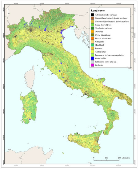
Figure 3. Land cover map of Italy for 2012.

Accuracy assessment was conducted on the map of Figure 3 and provides the results shown in Figure 4 and summarized in Table 10. The map has an overall accuracy of 90%. The omission error is less than 20% in all classes and slightly higher than this value for permanent snow and ice and wetlands.

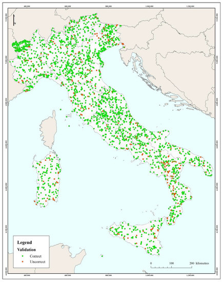
Figure 4. Result of the accuracy assessment with reference to the sample of photo-interpreted points.

Table 10. Overall, user and producer accuracy of the 2012 land cover map.

Overall Accuracy
0.83
Class name	User’s accuracy	Producer’s accuracy
Artificial abiotic surfaces	0.98	0.83
Consolidated (bare rocks scree, cliffs)	0.89	0.82
Unconsolidated (beaches, dunes, sands)	0.97	0.85
Broad-leaved	0.92	0.91
Needle-leaved	0.88	0.96
Orchards	0.82	0.86
Olive plantation	0.98	0.94
Wood plantations	0.90	0.84
Vineyards	0.79	0.89
Shrubland	0.84	0.83
Pastures	0.88	0.93
Arable land	0.92	0.93
Permanent herbaceous	0.76	0.83
Water bodies	0.90	0.95
Permanent snow and ice	0.99	0.79
Wetlands	0.88	0.79

The commission error is just over 20% in two of the 16 classes, while it is less than 3% for the artificial abiotic surfaces, beaches, dunes and sands, olive groves and permanent snow and ice.

Analyzing the first classification level of the 2012 land cover map, over 88% of the national surface is vegetated, followed by abiotic surfaces (9.83%) and water bodies and wetlands (1.46 and 0.16%). At the second classification level, in the abiotic class the artificial component prevails (6.98%) followed by bare rocks. Regarding vegetation, woody and herbaceous vegetation show comparable surfaces (45.7% and 42.7% respectively). In the woody class the arboreal component prevails, which occupies 38.91% of the national surface (Table 11).

Table 11. Land cover classes 2012 (first and second classification level).

		ha	% Total	% Class
Abiotic Surfaces		2,964,151	9.83
	Artificial abiotic surfaces	802,539	2.66	27.07
	Natural abiotic surfaces	59,325	0.20	2.00
Bioticvegetated		26,685,696	88.54
	Woody vegetation	13,791,561	45.76	51.68
	Herbaceous vegetation	12,894,135	42.78	48.32
Water surfaces		439,830	1.46
	Water bodies	402,830	1.34	91.59
	Permanent snow and ice	37,000	0.12	8.41
Wetlands		50,295	0.17

Considering the maximum thematic detail, class 2212 (arable land) prevail, which occupies 30.47% of the national territory, followed by broad-leaved trees (25.90%). All other classes occupy less than 10% of the territory and 11 out of 16 classes less than 5% (Table 12).

Table 12. Land cover classes 2012 (up to fifth classification level).

LC Code	Class Name	ha	%
11000	Artificial abiotic surfaces	2,102,288	6.98
12100	Consolidated (bare rocks scree, cliffs)	802,539	2.66
12200	Unconsolidated (beaches, dunes, sands)	59,325	0.20
21110	Broad-leaved	7,805,217	25.90
21120	Needle-leaved	2,167,261	7.19
21131	Orchards	619,759	2.06
21132	Olive plantations	1,088,099	3.61
21133	Wood plantations	46,356	0.15
21210	Vineyards	689,746	2.29
21220	Shrubland	1,375,125	4.56
22110	Pastures	1,372,790	4.55
22120	Arable land	9,183,519	30.47
22200	Permanent herbaceous	2,337,826	7.76
31000	Water bodies	402,830	1.34
32000	Permanent snow and ice	37,000	0.12
40000	Wetlands	50,295	0.17
Total		30,139,972	100.00

3.2. Estimation of the Carbon Storage Capacity

The application to the 2012 map of the methodology for calculating the carbon stocks obtained the results shown in Figure 5, which show a strong concentration of the carbon stocks in the alpine and mountain areas, while the value is significantly reduced in the agricultural areas of the Padana plain and in particular in Sicily and in the Tavoliere delle Puglie.

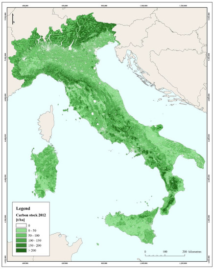
Figure 5. Carbon stock (2012).

In Italy, 2,898,672 tons of stored carbon (stock) were lost due to land consumption between 2012 and 2020 (Table 13). In detail, this value relates to transformations from natural to artificial land cover, excluding restorations and changes between other different land cover classes. Analysing the results on a regional scale, almost a quarter of the total losses are concentrated in the Veneto (384,537 tons, equal to 13.27% of the total) and Lombardy (319,666 tons, 11.03% of the total), while each of the other regions is affected by less than 10% of the changes. The minor losses are in Aosta Valley (13,206 tons), Molise (21,242 tons) and Liguria (25,237 tons), which together host less than 2% of the changes.

Table 13. Variation in carbon storage capacity (2012–2020).

Region	C Storage Variation (2012–2020)
	(Tons)	(%)
Abruzzo	86.034	2.97
Basilicata	52.086	1.80
Calabria	102.138	3.52
Campania	200.661	6.92
Emilia-Romagna	274.205	9.46
Friuli-Venezia Giulia	91.222	3.15
Latium	203.818	7.03
Liguria	25.237	0.87
Lombardy	319.667	11.03
Marche	81.746	2.82
Molise	21.243	0.73
Piedmont	203.725	7.03
Apulia	210.723	7.27
Sardinia	88.891	3.07
Sicily	225.972	7.80
Tuscany	120.143	4.14
Trentino-South Tyrol	134.470	4.64
Umbria	58.947	2.03
Aosta Valley	13.207	0.46
Veneto	384.537	13.27
Italy	2.898.672	100.00

4. Discussion

The effectiveness of ecosystem services assessment methodologies is linked to the availability of spatial data that allow an accurate and reliable description of the territory [59,60].

The CLC is still one of the few data able to guarantee information on land cover and land use for the entire national territory and is a reference for studies on a national scale. However, the new monitoring needs in terms of updating frequency and spatial resolution have revealed the limits of the project. The increase in geometric detail guaranteed by the introduction of high resolution data from the Copernicus local component and national data made it possible to describe the territory more accurately than the CLC in critical areas, such as urban areas, riparian areas and protected areas, although important portions of the national territory are still covered only by CLC.

Figure 6 shows a more detailed representation of green urban areas, which is relevant if we consider that the ecosystem functions and services that urban soils are able to offer are often neglected [61].

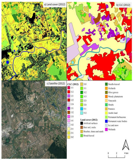
Figure 6. Comparison between land cover map for 2012 (a), CORINE Land Cover (b) and satellite image (c), focusing on urban area.

The increase in geometric detail also makes it possible to improve the representation of small urban agglomerations, roads and riparian areas (Figure 6, Figure 7, Figure 8 and Figure 9).

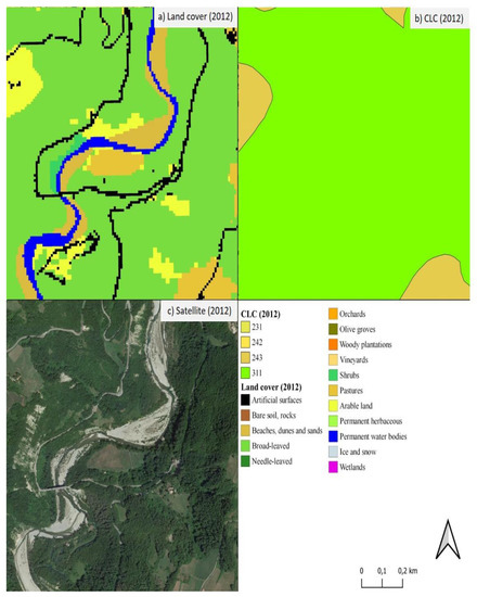
Figure 7. Comparison between land cover map for 2012 (a), CORINE Land Cover (b) and satellite image (c), focusing on water courses.

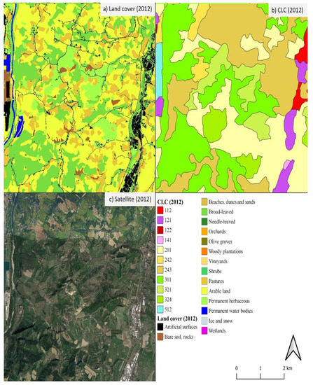
Figure 8. Comparison between land cover map for 2012 (a), CORINE Land Cover (b) and satellite image (c), focusing on small patches of natural vegetation and agricultural areas.

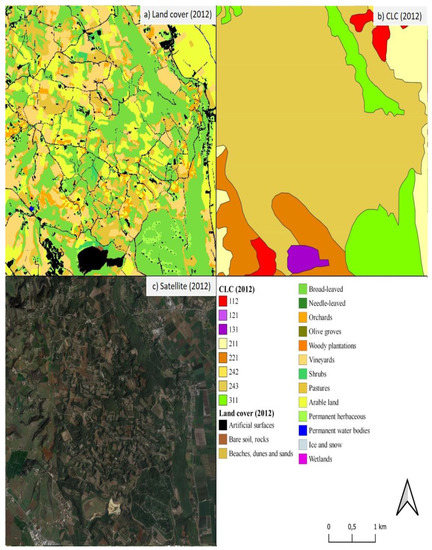
Figure 9. Comparison between land cover map for 2012 (a), CORINE Land Cover (b) and satellite image (c), focusing on heterogeneous agricultural areas.

Anyway, all the Copernicus data used for this research present critical issues from a thematic point of view, since their classification system is based on land cover and land use attributes with numerous mixed classes, such as the CLC class 2.4 (heterogeneous agricultural areas) and 3.2 (shrub and/or herbaceous vegetation associations).

The proposed methodology allows a more detailed description of the mixed classes, (Figure 8 and Figure 9) and makes it possible to distinguish the arboreal component from the herbaceous one, the agricultural areas from the natural ones, arable land from permanent crops. That allows the carbon storage capacity of the different classes to be analysed separately and more accurately. Although aspects such as the diameter of the trunk, the density of the trees or the characteristics of the undergrowth are not considered, the map distinguishes the tree species in a detailed way, maintaining the fourth classification level of CLC, which is available only for the Italian territory [62].

An aspect that will require further development is the possibility of defining the correspondence between the classes of Copernicus data and a classification system oriented to the description of habitats, which would be more functional for conducting studies on ecosystem services. In this sense it would be necessary to integrate ancillary data not easily available on a national scale [63].

The data available at the time of the research limited the study on carbon stocks only to variations caused by increased land consumption. The availability of new Copernicus data updated to 2018 will allow the production of land cover maps capable of evaluating the variations of ecosystem services associated with other land cover changes occurred between 2012 and 2018 [60]. However the update frequency remains too low for numerous monitoring activities. Actually, the LCM is updated annually, while Copernicus data every 6 years and the maps available at regional level in Italy are often based on CLC data and are updated in a few cases (Lombardy, updated to 2018, Tuscany 2016, Liguria 2018, Latium 2016), while other maps are less up to date (2012 for Sicily and Apulia, 2013 for Abruzzo and Basilicata, 2006 for Calabria and 2009 for Campania).

Initiatives such as the next “CLC Plus” are expected to be decisive in the near future, guaranteeing the introduction of updated and interoperable products, more suitable for carrying out the monitoring activities necessary to meet institutional needs. ISPRA is conducting other research activities in this direction [41,43,44,45,64], through the definition of a land cover classification methodology for the production of maps with Sentinel resolution, annual update frequency and EAGLE compliant classification system, capable of providing updated and reliable products for monitoring on a national scale, which can be integrated with the activities of the “CLC Plus” and the National Strategic Plan for the Space Economy.

5. Conclusions

Since the 19th century, anthropogenic activities have led to a significant increase in the level of carbon dioxide in the atmosphere [35] and negatively affected the regeneration capacity and balance of ecosystems. Urban expansion, deforestation and forest degradation have contributed to these emissions by releasing the carbon stored naturally in forests, vegetation and soil [34,35]. This type of carbon is added to greenhouse gas emissions related to industries and energy production and to the products of impure combustion. Terrestrial ecosystems are able to sequester as much carbon as is currently in the atmosphere but over the course of the century terrestrial biosphere is likely to become a net source of carbon due to factors connected with climate change, pollution and the over-exploitation of resources that will alter the structure, reduce biodiversity and perturb functioning of most ecosystems, and compromise the services they currently provide.

The land cover and land use changes involve landscape fragmentation, reduction of biodiversity and loss of green areas important for carbon accumulation and more generally for the provision of ecosystem services. Current conservation practices are generally poorly prepared to adapt to this level of change, and effective adaptation responses are likely to be costly to implement.

The monitoring of carbon stock accounting is an institutional duty enshrined in the Kyoto protocol and the Paris agreements and an important driver in defining adaptation strategies to climate change [33]. Effective monitoring strategies of land cover and land use changes are essential for studying the phenomenon. In this sense, the methodology presented in this paper represents a step forward for large-scale assessments of ecosystem services more relevant to reality, since compared to the CLC it provides products for the entire national territory with greater geometric detail and a better description of mixed areas.

The methodology is easily applicable in other territorial areas, since it is based on Copernicus data available for many European countries, furthermore the use of an EAGLE compliant classification system makes the methodology easily adaptable to the specific availability of national data.

The main limitation of the methodology concerns the low update frequency of the input data, which limited the monitoring of ecosystem services to variations related to land consumption, which is the only data updated annually for the Italian territory.

A first future development concerns the updating of the map using the new Copernicus Local and Pan-European products for 2018. This implementation will allow the evaluation of the variations in the carbon stocks associated not only with land consumption but also with other land cover changes.

The products of the application of the methodology are also in continuity with other activities carried out by the working group and can constitute a useful support tool for the development of land cover classification methodologies with high update frequency for the satisfaction of the institutional needs envisaged by the new “Space Economy” Strategic Plan and for the creation of “Istances” in the new CLC Plus Project. In this sense, an important added value of this research is linked to the suitability of products with respect to present and future national and European initiatives and standards in the field of remote sensing.

References

- Munafò, M. Consumo di Suolo, Dinamiche Territoriali e Servizi Ecosistemici—Edizione 2018; ISPRA: Rome, Italy, 2018. [Google Scholar]
- Verburg, P.H.; Erb, K.-H.; Mertz, O.; Espindola, G. Land System Science: Between global challenges and local realities. Curr. Opin. Environ. Sustain. 2013, 5, 433–437. [Google Scholar] [CrossRef] [PubMed] [Green Version]
- Pedroli, G.B.M.; Meiner, A. Landscapes in Transition: An Account of 25 Years of Land Cover Change in Europe; European Environment Agency: København, Denmark, 2017. [Google Scholar]
- EEA. Land Systems at European Level—Analytical Assessment Framework. 2018. Briefing no. 10/2018. pp. 1–9. Available online: https://www.eea.europa.eu/themes/landuse/land-systems (accessed on 28 November 2021).
- Anderson, J.R. Land use and land cover changes. A framework for monitoring. J. Res. Geol. Surv. 1977, 5, 143–153. [Google Scholar]
- Liu, R.; Dong, X.; Wang, X.; Zhang, P.; Liu, M.; Zhang, Y. Study on the relationship among the urbanization process, ecosystem services and human well-being in an arid region in the context of carbon flow: Taking the Manas river basin as an example. Ecol. Indic. 2021, 132, 108248. [Google Scholar] [CrossRef]
- Costanza, R.; D’Arge, R.; de Groot, R.; Farberll, S.; Grassot, M.; Hannon, B.; Limburg, K.; Naeem, S.; O’Neilltt, R.V.; Paruelo, J.; et al. The value of the world’s ecosystem services and natural capital. Nature 1997, 387115, 253–260. [Google Scholar] [CrossRef]
- Gómez-Baggethun, E.; De Groot, R.; Lomas, P.L.; Montes, C. The history of ecosystem services in economic theory and practice: From early notions to markets and payment schemes. Ecol. Econ. 2010, 69, 1209–1218. [Google Scholar] [CrossRef]
- Danley, B.; Widmark, C. Evaluating conceptual definitions of ecosystem services and their implications. Ecol. Econ. 2016, 126, 132–138. [Google Scholar] [CrossRef]
- Teague, A.; Russell, M.; Harvey, J.; Dantin, D.; Nestlerode, J.; Alvarez, F. A spatially-explicit technique for evaluation of alternative scenarios in the context of ecosystem goods and services. Ecosyst. Serv. 2016, 20, 15–29. [Google Scholar] [CrossRef]
- Corvalan, C.; Hales, S.; McMichael, A.; Butler, C.; Campbell-Lendrum, D.; Confalonieri, U.; Leitner, K.; Lewis, N.; Patz, J.; Polson, K.; et al. A Report of the Millennium Ecosystem Assessment. In Ecosystems and Human Well-Being; Island Press: Washington, DC, USA, 2005; Volume 5. [Google Scholar]
- Xepapadeas, A. The Economics of Ecosystems and Biodiversity: Ecological and Economic Foundations; Kumar, P., Ed.; Earthscan: London, UK; Washington, DC, USA, 2011; Volume 16, pp. 239–242. ISBN 978-1-84971-212-5 (HB). [Google Scholar]
- La Notte, A.; D’Amato, D.; Mäkinen, H.; Paracchini, M.L.; Liquete, C.; Egoh, B.; Geneletti, D.; Crossman, N.D. Ecosystem services classification: A systems ecology perspective of the cascade framework. Ecol. Indic. 2017, 74, 392–402. [Google Scholar] [CrossRef]
- Potschin, M.; Haines-Young, R. Defining and measuring ecosystem services. In Routledge Handbook of Ecosystem Services; Potschin, M., Haines-Young, R., Fish, R., Turner, R.K., Eds.; Routledge: London, UK; New York, NY, USA, 2016; pp. 25–44. [Google Scholar]
- Costanza, R.; de Groot, R.; Sutton, P.; van der Ploeg, S.; Anderson, S.J.; Kubiszewski, I.; Farber, S.; Turner, R.K. Changes in the global value of ecosystem services. Glob. Environ. Chang. 2014, 26, 152–158. [Google Scholar] [CrossRef]
- Zulian, G.; Maes, J.; Paracchini, M.L. Linking land cover data and crop yields for mapping and assessment of pollination services in Europe. Land 2013, 2, 472–492. [Google Scholar] [CrossRef] [Green Version]
- Groff, S.C.; Loftin, C.S.; Drummond, F.; Bushmann, S.; McGill, B. Parameterization of the InVEST crop pollination model to spatially predict abundance of wild blueberry (Vaccinium angustifolium Aiton) native bee pollinators in Maine, USA. Environ. Model. Softw. 2016, 79, 1–9. [Google Scholar] [CrossRef] [Green Version]
- Leonhardt, S.D.; Gallai, N.; Garibaldi, L.A.; Kuhlmann, M.; Klein, A.-M. Economic gain, stability of pollination and bee diversity decrease from southern to northern Europe. Basic Appl. Ecol. 2013, 14, 461–471. [Google Scholar] [CrossRef]
- Lautenbach, S.; Seppelt, R.; Liebscher, J.; Dormann, C.F. Spatial and temporal trends of global pollination benefit. PLoS ONE 2012, 7, e35954. [Google Scholar] [CrossRef] [PubMed] [Green Version]
- Hanley, N.; Breeze, T.D.; Ellis, C.; Goulson, D. Measuring the economic value of pollination services: Principles, evidence and knowledge gaps. Ecosyst. Serv. 2015, 14, 124–132. [Google Scholar] [CrossRef] [Green Version]
- UK National Ecosystem Assessment. The UK National Ecosystem Assessment: Synthesis of the Key Findings; UNEP-WCMC: Cambridge, UK, 2011. [Google Scholar]
- Rabe, S.-E.; Koellner, T.; Marzelli, S.; Schumacher, P.; Grêt-Regamey, A. National ecosystem services mapping at multiple scales. The German exemplar. Ecol. Indic. 2016, 70, 357–372. [Google Scholar] [CrossRef]
- Santos-Martín, F.; García Llorente, M.; Quintas-Soriano, C.; Zorrilla-Miras, P.; Martín-Lopez, B.; Loureiro, M.; Benayas, J.; Montes, M. Spanish National Ecosystem Assessment: Socio-economic valuation of ecosystem services in Spain. Synthesis of the key findings; Biodiversity Foundation of the Spanish Ministry of Agriculture, Food and Environment: Madrid, Spain, 2016.
- Xie, G.; Zhang, C.; Zhen, L.; Zhang, L. Dynamic changes in the value of China’s ecosystem services. Ecosyst. Serv. 2017, 26, 146–154. [Google Scholar] [CrossRef]
- Turpie, J.K.; Forsythe, K.J.; Knowles, A.; Blignaut, J.; Letley, G. Mapping and valuation of South Africa’s ecosystem services: A local perspective. Ecosyst. Serv. 2017, 27, 179–192. [Google Scholar] [CrossRef]
- Choi, H.-A.; Song, C.; Lee, W.-K.; Jeon, S.; Gu, J.H. Integrated approaches for national ecosystem assessment in South Korea. KSCE J. Civ. Eng. 2018, 22, 1634–1641. [Google Scholar] [CrossRef]
- Daily, G.C.; Matson, P.A.; Vitousek, P.M. Ecosystem services supplied by soil. In Nature’s Services: Societal Dependence on Natural Ecosystems; Daily, G.C., Ed.; Island Press: Washington, DC, USA, 1997; pp. 113–132. [Google Scholar]
- Wall, D.H.; Bardgett, R.D.; Covich, A.P.; Snelgrove, P.V.R. The Need for Understanding How Biodiversity and Ecosystem Functioning Affect Ecosystem Services in Soils and Sediments; Island Press: Washington, DC, USA, 2004. [Google Scholar]
- Dominati, E.; Patterson, M.; Mackay, A. A framework for classifying and quantifying the natural capital and ecosystem services of soils. Ecol. Econ. 2010, 69, 1858–1868. [Google Scholar] [CrossRef]
- Fryer, J.; Williams, I.D. Regional carbon stock assessment and the potential effects of land cover change. Sci. Total Environ. 2021, 775, 145815. [Google Scholar] [CrossRef] [PubMed]
- Mathew, I.; Shimelis, H.; Mutema, M.; Minasny, B.; Chaplot, V. Crops for increasing soil organic carbon stocks–A global meta analysis. Geoderma 2020, 367, 114230. [Google Scholar] [CrossRef]
- Clerici, N.; Cote-Navarro, F.; Escobedo, F.J.; Rubiano, K.; Villegas, J.C. Spatio-temporal and cumulative effects of land use-land cover and climate change on two ecosystem services in the Colombian Andes. Sci. Total Environ. 2019, 685, 1181–1192. [Google Scholar] [CrossRef]
- Savaresi, A.; Perugini, L.; Chiriacò, M.V. Making sense of the LULUCF Regulation: Much ado about nothing? Rev. Eur. Comp. Int. Environ. Law 2020, 29, 212–220. [Google Scholar] [CrossRef]
- Sallustio, L.; Quatrini, V.; Geneletti, D.; Corona, P.; Marchetti, M. Assessing land take by urban development and its impact on carbon storage: Findings from two case studies in Italy. Environ. Impact Assess. Rev. 2015, 54, 80–90. [Google Scholar] [CrossRef] [Green Version]
- Vashum, K.T.; Jayakumar, S. Methods to estimate above-ground biomass and carbon stock in natural forests-a review. J. Ecosyst. Ecography 2012, 2, 1–7. [Google Scholar] [CrossRef]
- Sallustio, L.; Munafò, M.; Riitano, N.; Lasserre, B.; Fattorini, L.; Marchetti, M. Integration of land use and land cover inventories for landscape management and planning in Italy. Environ. Monit. Assess. 2016, 188, 48. [Google Scholar] [CrossRef]
- Maes, J.; Teller, A.; Erhard, M.; Liquete, C.; Braat, L.; Berry, P.; Egoh, B.; Puydarrieus, P.; Fiorina, C.; Santos, F.; et al. An Analytical Framework for Ecosystem Assessments under Action 5 of the EU Biodiversity Strategy to 2020; Publications Office of the European Union: Luxembourg, 2013; ISBN 9789279293696. [Google Scholar]
- Cabral, P.; Feger, C.; Levrel, H.; Chambolle, M.; Basque, D. Assessing the impact of land-cover changes on ecosystem services: A first step toward integrative planning in Bordeaux, France. Ecosyst. Serv. 2016, 22, 318–327. [Google Scholar] [CrossRef] [Green Version]
- Arnold, S.; Kosztra, B.; Banko, G.; Smith, G.; Hazeu, G.; Bock, M. The EAGLE concept—A vision of a future European Land Monitoring Framework. In Proceedings of the 33th EARSeL Symposium towards Horizon 2020, Matera, Italy, 3–6 June 2013; pp. 551–568. [Google Scholar]
- Kleeschulte, S. Technical Specifications for Implementation of a New Land-Monitoring Concept Based on EAGLE. D3: Draft Design Concept and CLC-Backbone, CLC-Core Technical Specifications, Including Requirements Review, 3rd ed.; European Environment Agency: Copenhagen, Denmark, 2019; p. 78. [Google Scholar]
- De Fioravante, P.; Luti, T.; Cavalli, A.; Giuliani, C.; Dichicco, P.; Marchetti, M.; Chirici, G.; Congedo, L.; Munafò, M. Multispectral Sentinel-2 and SAR Sentinel-1 Integration for Automatic Land Cover Classification. Land 2021, 10, 611. [Google Scholar] [CrossRef]
- Munafò, M. Consumo di Suolo, Dinamiche Territoriali e Servizi Ecosistemici. Edizione 2020; ISPRA: Rome, Italy, 2020. [Google Scholar]
- Munafò, M. Consumo di Suolo, Dinamiche Territoriali e Servizi Ecosistemici Edizione 2021 Rapporto ISPRA SNPA; ISPRA: Rome, Italy, 2021; ISBN 9788844810597. [Google Scholar]
- Luti, T.; De Fioravante, P.; Marinosci, I.; Strollo, A.; Riitano, N.; Falanga, V.; Mariani, L.; Congedo, L.; Munafò, M. Land Consumption Monitoring with SAR Data and Multispectral Indices. Remote Sens. 2021, 13, 1586. [Google Scholar] [CrossRef]
- Strollo, A.; Smiraglia, D.; Bruno, R.; Assennato, F.; Congedo, L.; De Fioravante, P.; Giuliani, C.; Marinosci, I.; Riitano, N.; Munafò, M. Land consumption in Italy. J. Maps 2020, 16, 113–123. [Google Scholar] [CrossRef]
- Olofsson, P.; Foody, G.M.; Herold, M.; Stehman, S.V.; Woodcock, C.E.; Wulder, M.A. Good practices for estimating area and assessing accuracy of land change. Remote Sens. Environ. 2014, 148, 42–57. [Google Scholar] [CrossRef]
- FAO Map Accuracy Assessment and Area Estimation: A Practical Guide. National Forest Monitoring and Assessment Working Paper. 2016. 46/E. p. 69. Available online: https://www.fao.org/publications/card/fr/c/e5ea45b8-3fd7-4692-ba29-fae7b140d07e/ (accessed on 28 November 2021).
- Stehman, S.V.; Czaplewski, R.L. Design and Analysis for Thematic Map Accuracy Assessment—An application of satellite imagery. Remote Sens. Environ. 1998, 64, 331–344. [Google Scholar] [CrossRef]
- Stehman, S.V.; Foody, G.M. Key issues in rigorous accuracy assessment of land cover products. Remote Sens. Environ. 2019, 231, 111199. [Google Scholar] [CrossRef]
- Cochran, W.G.; William, G. Sampling Techniques; John Wiley& Sons: New York, NY, USA, 1977. [Google Scholar]
- Lupia, F. MARSALa-A Model-Based Irrigation Water Consumption Estimation at Farm Level; INEA: Brussels, Belgium, 2013. [Google Scholar]
- Vitullo, M.; De Lauretis, R.; Federici, S. La Contabilità del Carbonio Contenuto Nelle Foreste Italiane; Agenzia per la Protezione dell’ambiente e per i Servizi Tecnici: Rome, Italy, 2007. [Google Scholar]
- Di Cosmo, L.; Gasparini, P.; Tabacchi, G. A national-scale, stand-level model to predict total above-ground tree biomass from growing stock volume. For. Ecol. Manag. 2016, 361, 269–276. [Google Scholar] [CrossRef]
- Romano, D.; Arcarese, C.; Bernetti, A.; Caputo, A.; Contaldi, M.; De Lauretis, R.; Di Cristofaro, E.; Gagna, A.; Gonella, B.; Taurino, E.; et al. Italian Greenhouse Gas Inventory 1990–2015. National Inventory Report 2017. 2017. Available online: https://www.isprambiente.gov.it/en/publications/reports/italian-greenhouse-gas-inventory-1990-2015.-national-inventory-report-2017 (accessed on 28 November 2021).
- Li, S.; Liu, Y.; Yang, H.; Yu, X.; Zhang, Y.; Wang, C. Integrating ecosystem services modeling into effectiveness assessment of national protected areas in a typical arid region in China. J. Environ. Manag. 2021, 297, 113408. [Google Scholar] [CrossRef]
- Penman, J.; Gytarsky, M.; Hiraishi, T.; Krug, T.; Kruger, D.; Pipatti, R.; Buendia, L.; Miwa, K.; Ngara, T.; Tanabe, K. Good practice guidance for land use, land-use change and forestry. Good Pract. Guid. L. Use Land-Use Chang. For. 2003. Available online: https://www.ipcc.ch/publication/good-practice-guidance-for-land-use-land-use-change-and-forestry/ (accessed on 28 November 2021).
- Marchetti, M.; Sallustio, L.; Ottaviano, M.; Barbati, A.; Corona, P.; Tognetti, R.; Zavattero, L.; Capotorti, G. Carbon sequestration by forests in the National Parks of Italy. Plant Biosyst. Int. J. Deal. Asp. Plant Biol. 2012, 146, 1001–1011. [Google Scholar] [CrossRef]
- Canaveira, P.; Manso, S.; Pellis, G.; Perugini, L.; De Angelis, P.; Neves, R.; Papale, D.; Paulino, J.; Pereira, T.; Pina, A. Biomass Data on Cropland and Grassland in the Mediterranean Region. Final Report for Action A4 of Project MediNet. 2018. Available online: http://www.lifemedinet.com/ (accessed on 28 November 2021).
- Burke, T.; Whyatt, J.D.; Rowland, C.; Blackburn, G.A.; Abbatt, J. The influence of land cover data on farm-scale valuations of natural capital. Ecosyst. Serv. 2020, 42, 101065. [Google Scholar] [CrossRef]
- Tomlinson, S.J.; Dragosits, U.; Levy, P.E.; Thomson, A.M.; Moxley, J. Quantifying gross vs. net agricultural land use change in Great Britain using the Integrated Administration and Control System. Sci. Total Environ. 2018, 628, 1234–1248. [Google Scholar] [PubMed]
- Morel, J.L.; Chenu, C.; Lorenz, K. Ecosystem services provided by soils of urban, industrial, traffic, mining, and military areas (SUITMAs). J. Soils Sediments 2015, 15, 1659–1666. [Google Scholar] [CrossRef]
- Sambucini, V.; Marinosci, I.; Bonora, N.; Chirci, G. La Realizzazione in Italia del Progetto CORINE Land Cover 2006; ISPRA: Rome, Italy, 2010; ISBN 9788844804770. [Google Scholar]
- Tomaselli, V.; Dimopoulos, P.; Marangi, C.; Kallimanis, A.S.; Adamo, M.; Tarantino, C.; Panitsa, M.; Terzi, M.; Veronico, G.; Lovergine, F. Translating land cover/land use classifications to habitat taxonomies for landscape monitoring: A Mediterranean assessment. Landsc. Ecol. 2013, 28, 905–930. [Google Scholar] [CrossRef] [Green Version]
- Spadoni, G.L.; Cavalli, A.; Congedo, L.; Munafò, M. Analysis of Normalized Difference Vegetation Index (NDVI) multi-temporal series for the production of forest cartography. Remote Sens. Appl. Soc. Environ. 2020, 20, 100419. [Google Scholar] [CrossRef]
Publisher’s Note: MDPI stays neutral with regard to jurisdictional claims in published maps and institutional affiliations. |
© 2021 by the authors. Licensee MDPI, Basel, Switzerland. This article is an open access article distributed under the terms and conditions of the Creative Commons Attribution (CC BY) license (https://creativecommons.org/licenses/by/4.0/).