
The Prediction of Carbon Emission Information in Yangtze River Economic Zone by Deep Learning

Abstract
:1. Introduction
2. Related Concepts and Algorithm Analysis
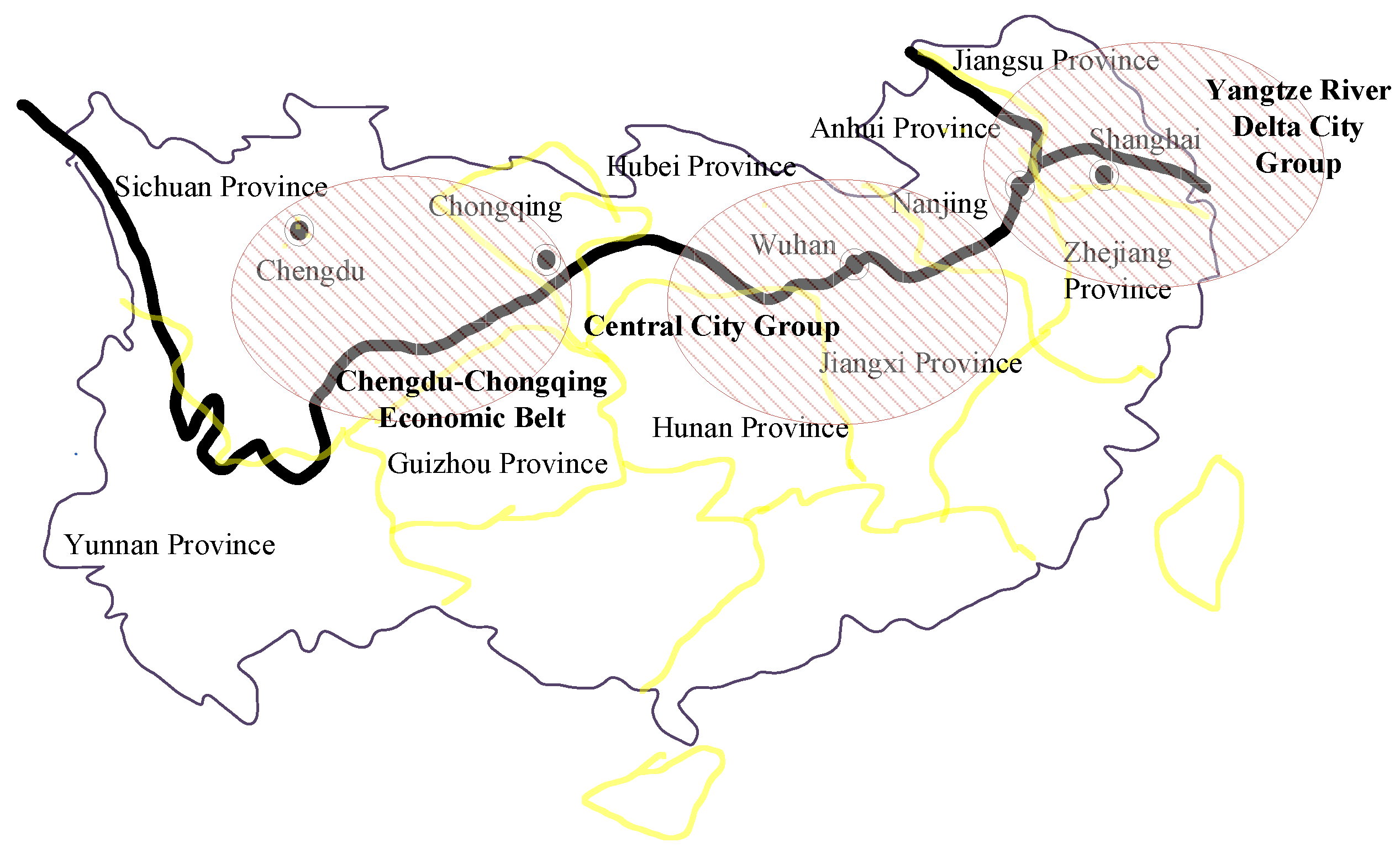
2.1. Yangtze River Economic Belt
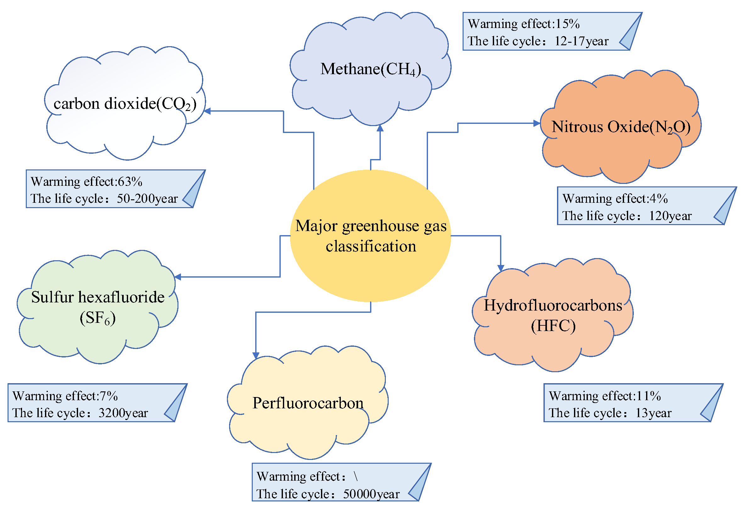
2.2. Definition and Analysis of Carbon Sources
2.2.1. Definition
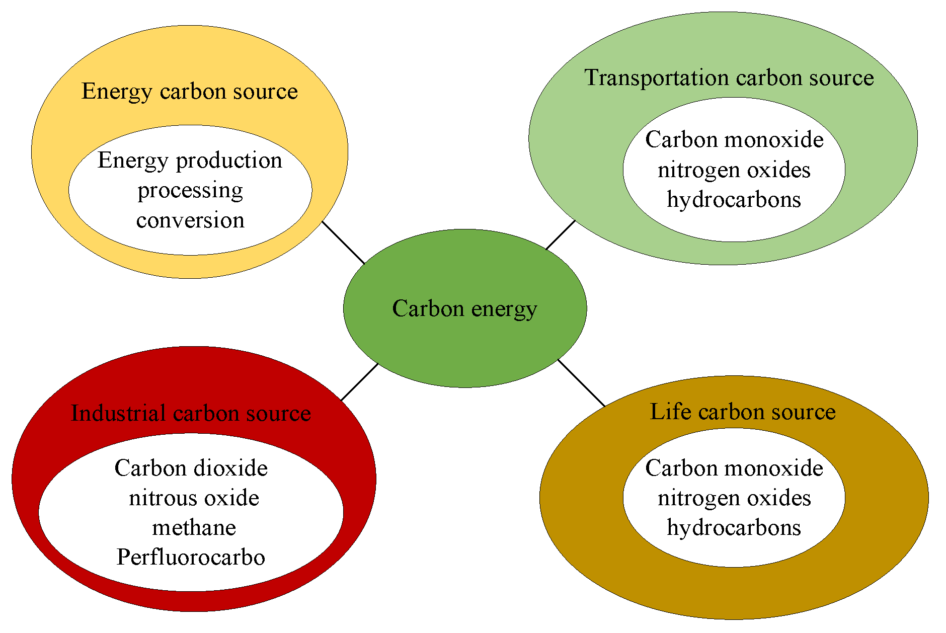
2.2.2. Analysis
2.2.3. Causes of Carbon Emissions
Carbon Emissions in the Process of Urbanization
Carbon Emissions from Animals and Plants
2.3. Algorithmic Analysis of Carbon Emissions
2.3.1. Oak Ridge National Laboratory (ORNL)
Fuel oil carbon emissions = standard coal equivalent × 0.982 × 0.733 × 0.813
Gas carbon emissions = standard coal equivalent × 0.982 × 0.733 × 0.561
2.3.2. Logistic Model
2.3.3. System Dynamics Model
2.3.4. Input–Output Analysis (IOA)
- Calculate the direct carbon emission coefficient: , where the energy carbon emission coefficient of the j sector is represented by as , that is, the CO2 emission per ton of energy, and is the energy consumption intensity of the j sector (10,000 tons of standard coal/CNY 10,000).
- Calculate the indirect carbon emission coefficient: , where the complete consumption of the i-sector product caused by the unit product is represented by . is the total indirect energy consumption of all n products caused by the unit product of the j sector. The complete carbon emission coefficient of energy consumption is equal to the sum of direct and indirect carbon emission coefficients, expressed as Equation (1):
2.4. Temporal and Spatial Characteristics of Carbon Emissions
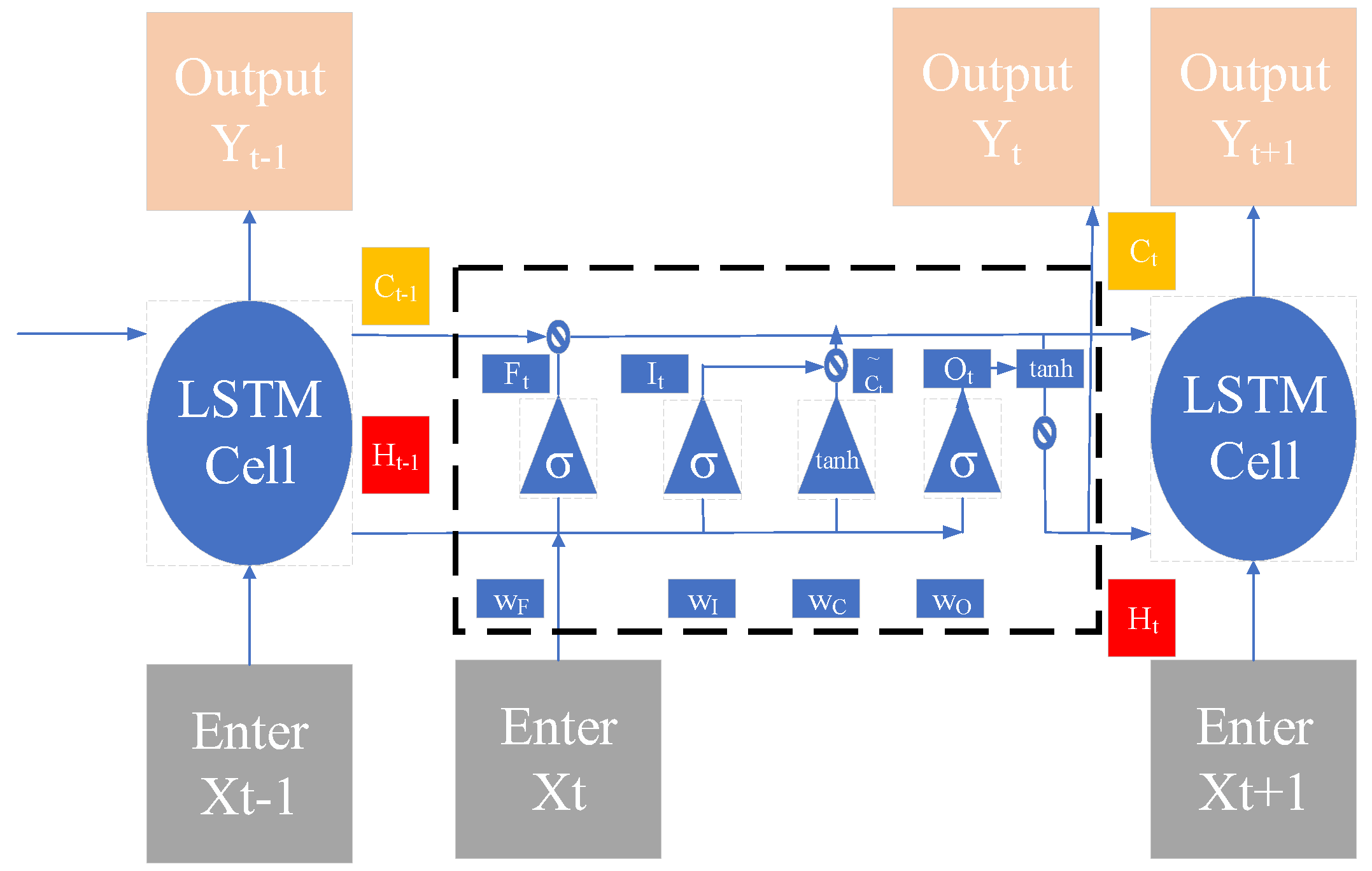
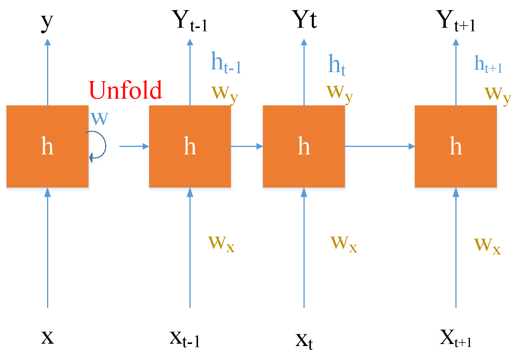
2.5. Analysis of Deep Learning Algorithms
- 1.
- Forgetting door calculation:
- 2.
- Input gate calculation:
- 3.
- Cell status update:
- 4.
- Output gate
3. Indicator Creation and Model Design
3.1. Creation of Carbon Emission Information Indicators
3.2. Carbon Emission Modeling Process
- (a)
- The MSE is the sum of squares of the difference between the results of the original feature data predicted by the model and the real results, but the sum of squares will continue to accumulate as the number of samples increases. In order to eliminate the influence of the number of samples, the mean value of the square error is calculated, and the MSE is obtained, as shown in Equation (15):
- (b)
- The average absolute error (MAE) is the average of the absolute value of the difference between the predicted value and the true value, as shown in Equation (16):
- (c)
- RMSE is shown Equation (17):
- (d)
- The absolute error of the median, the absolute value of the difference between the predicted value, and the true value are not averaged, but the median is taken, which is MedAE, as shown in Equation (18):
3.3. Data Source
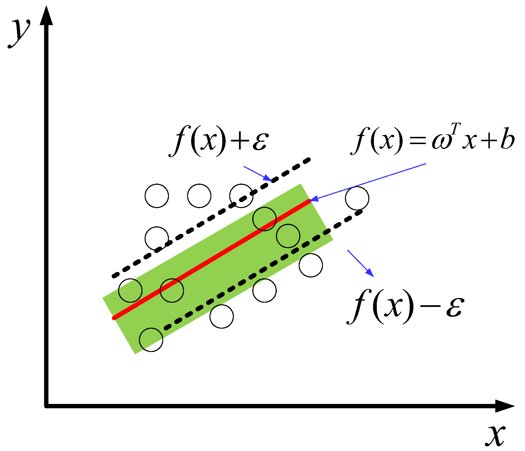
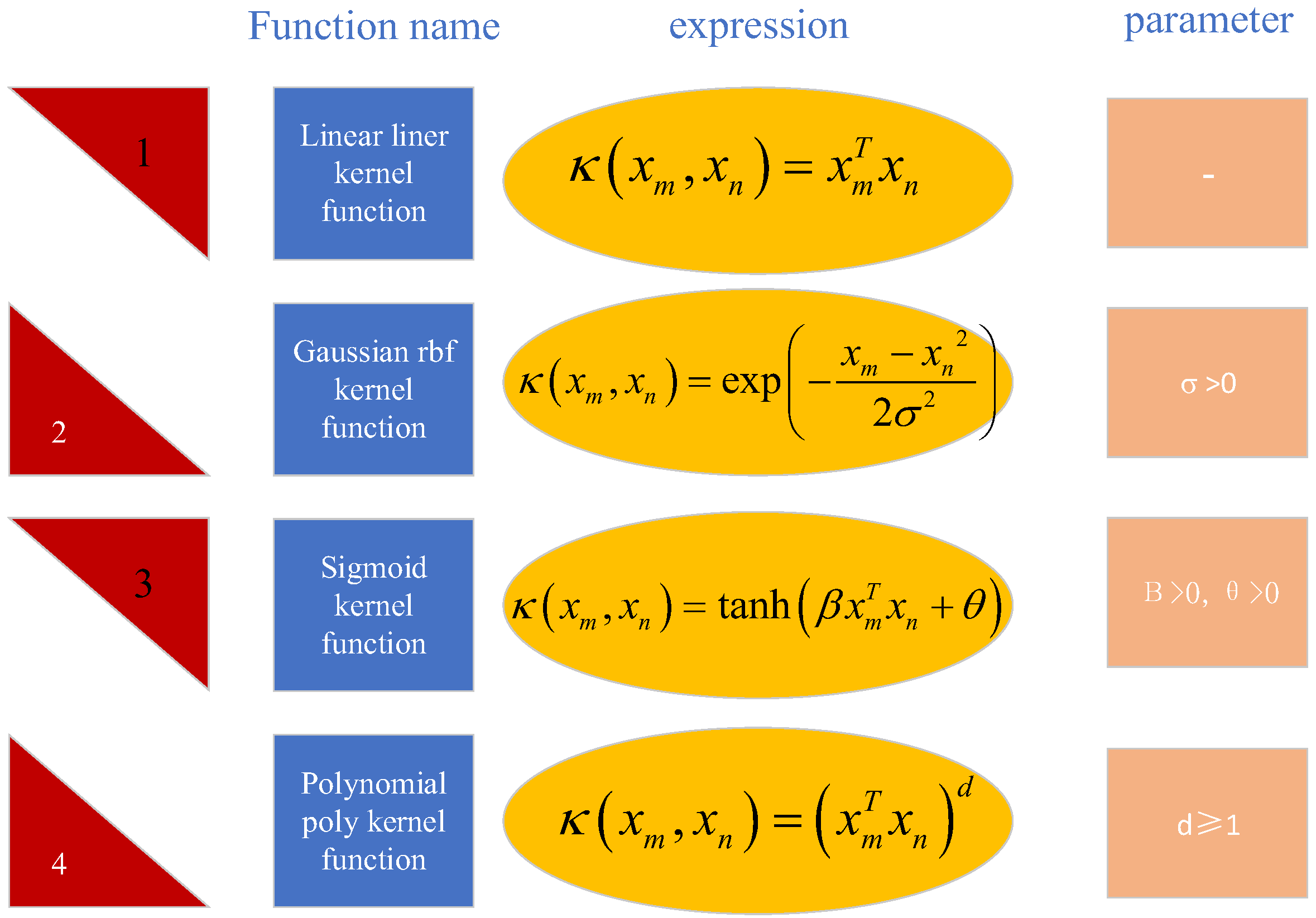
3.4. SVR Machine Model Creation
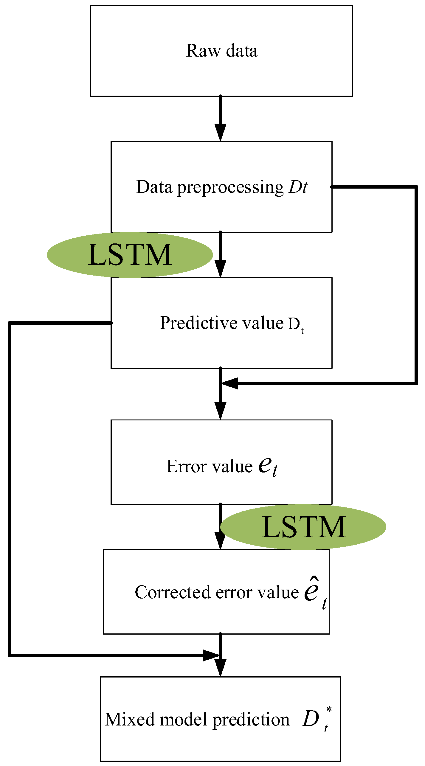
3.5. LSTM-SVR Hybrid Model Construction
4. Experimental Results and Analysis
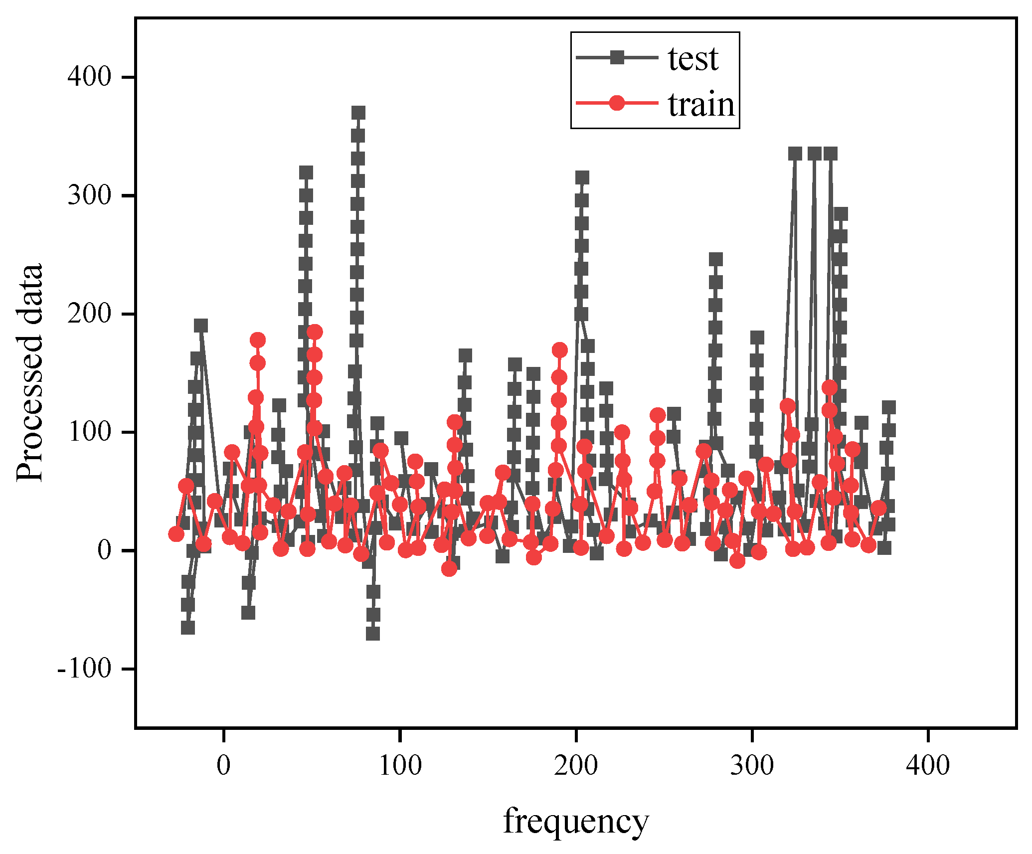
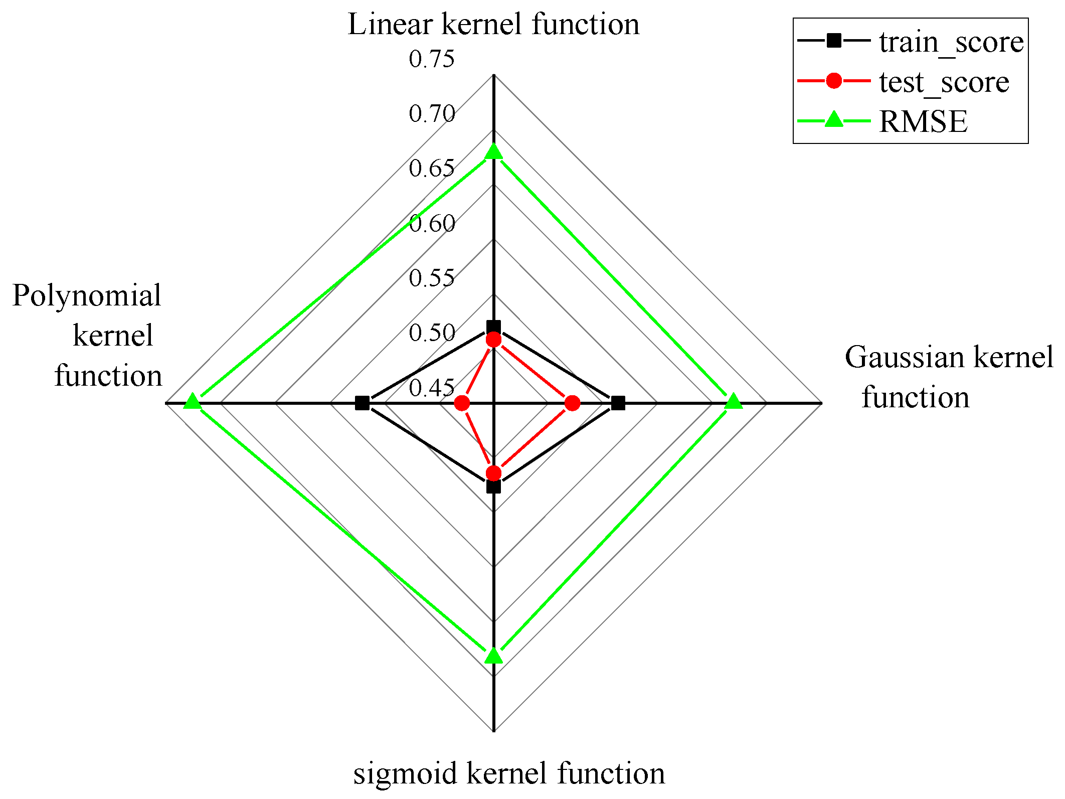
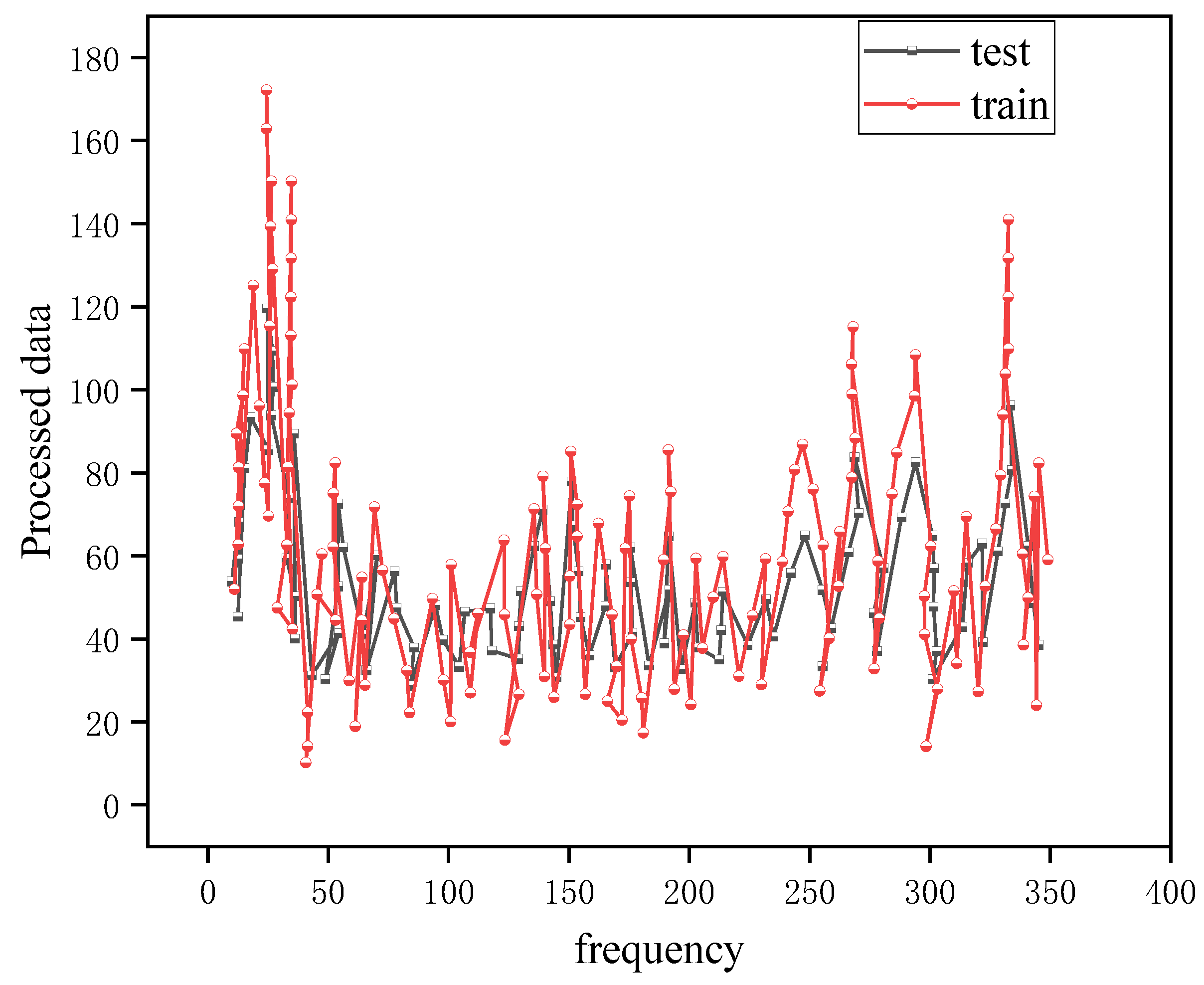
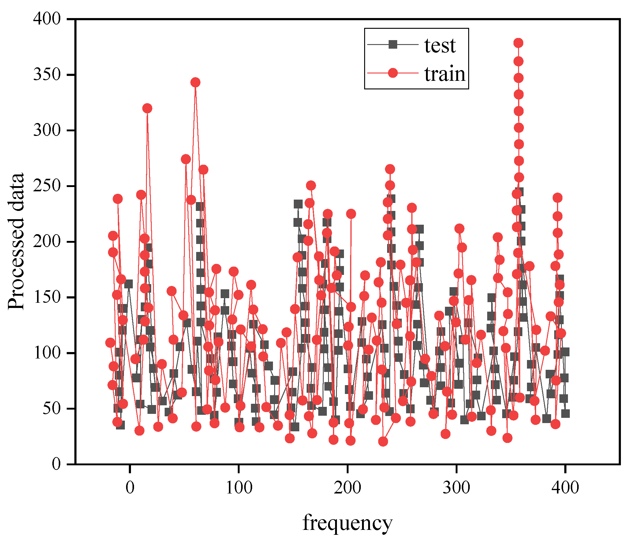
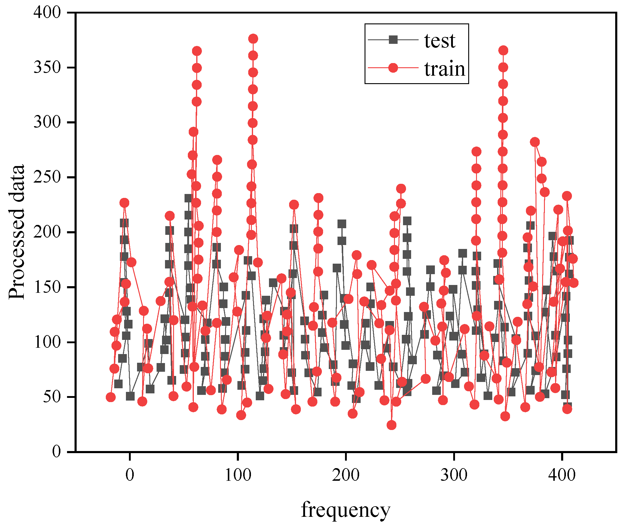
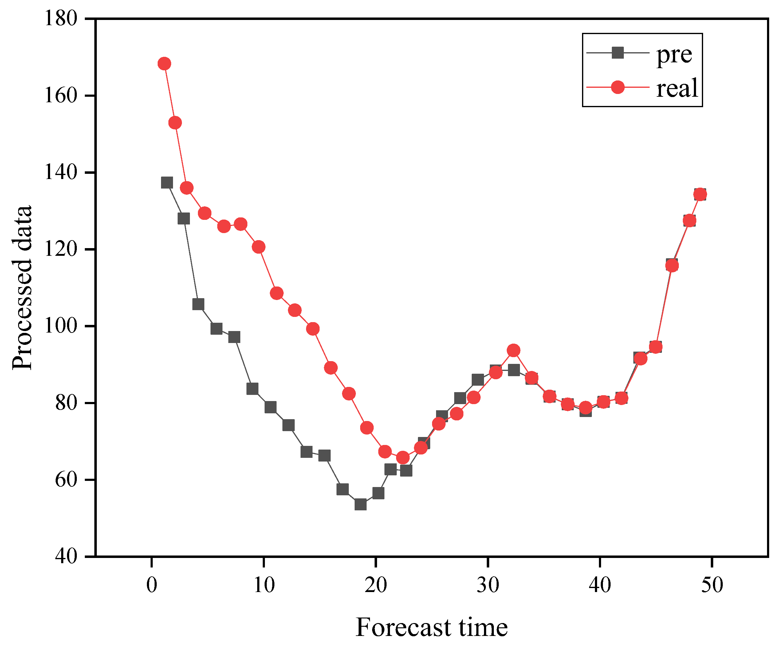
4.1. SVR Model Fitting Results
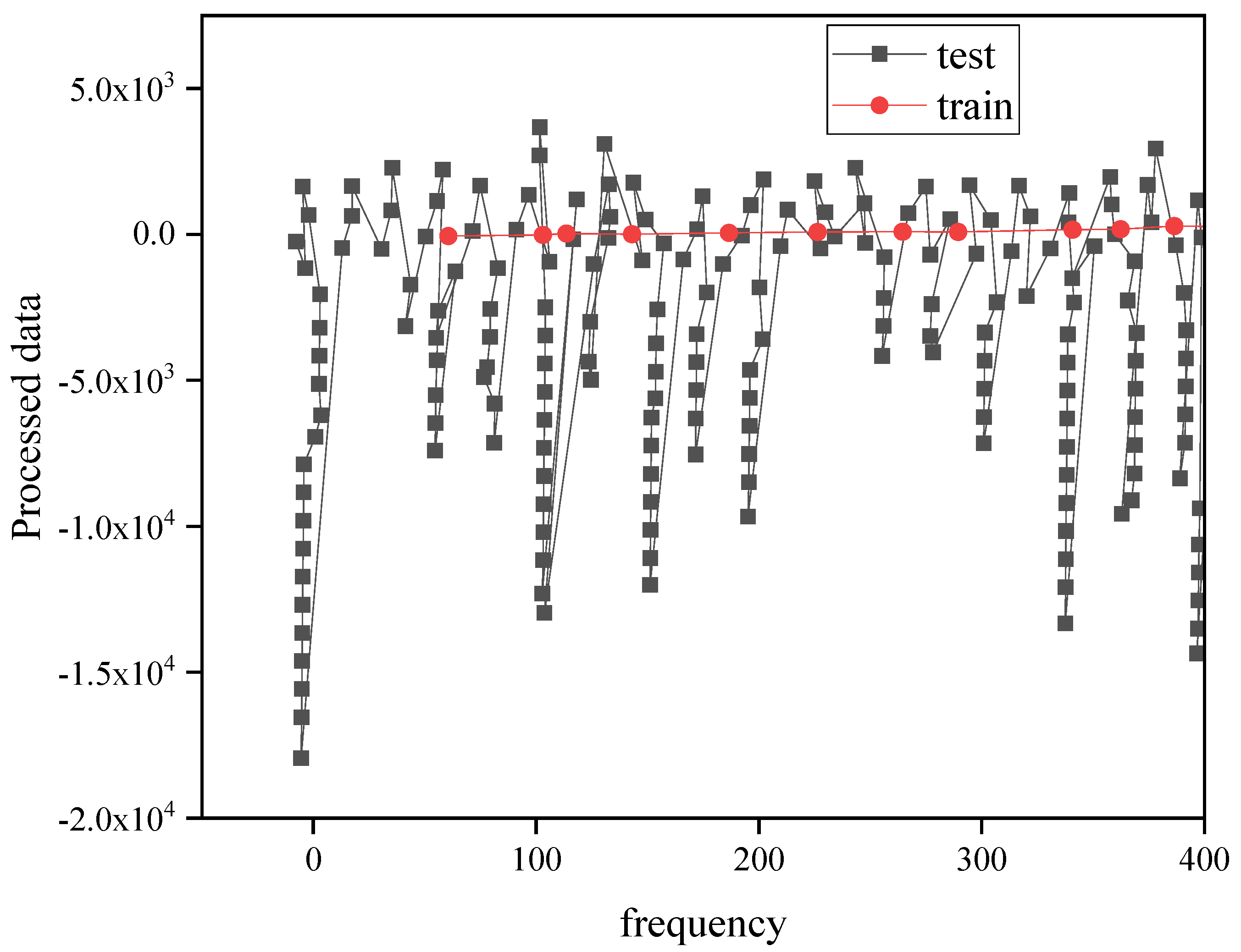
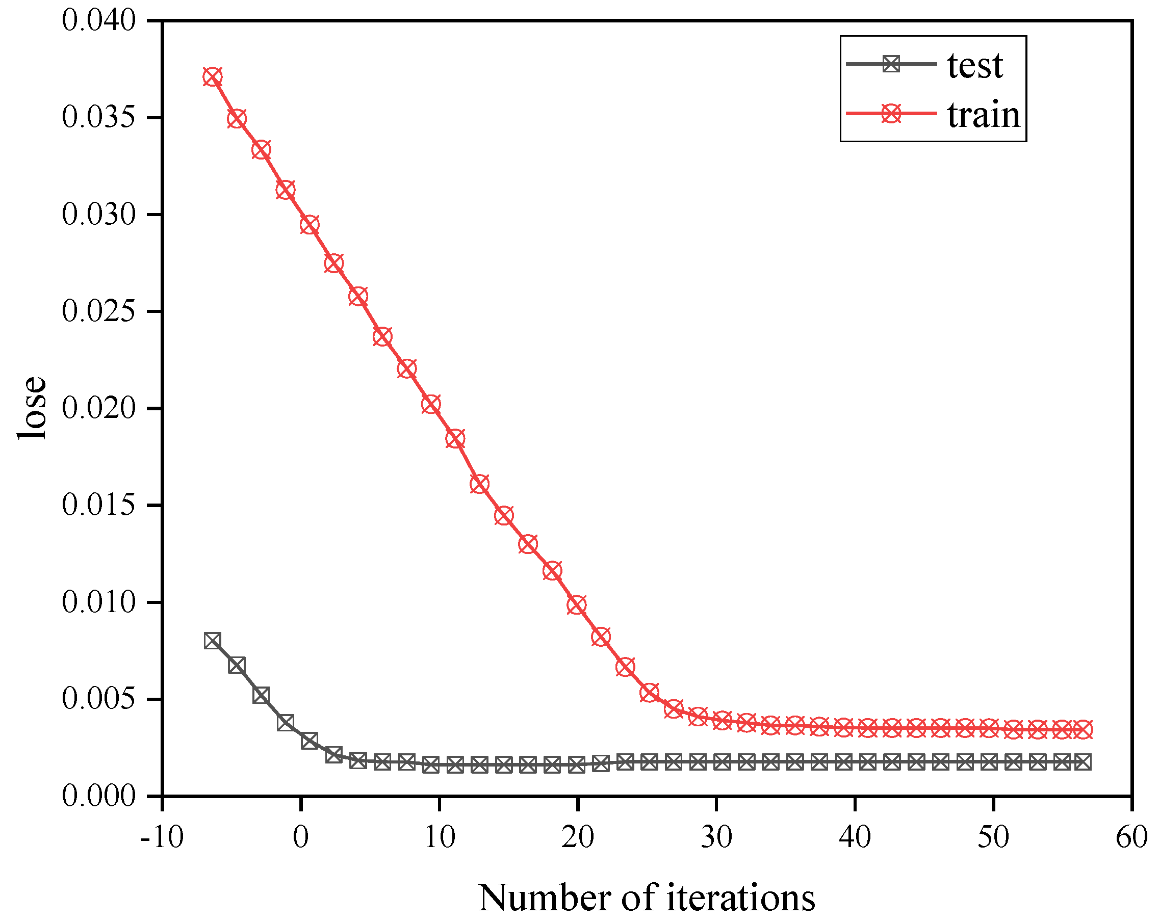
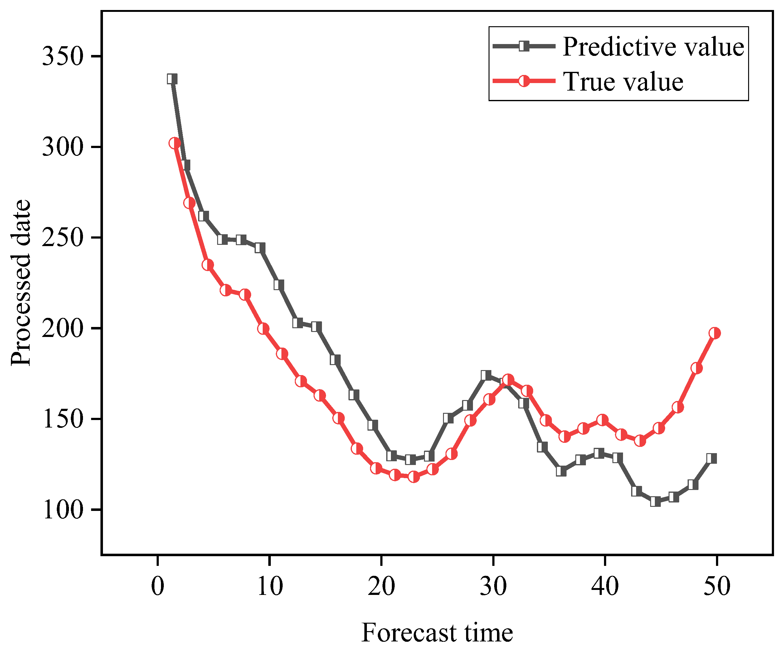
4.2. Deep Learning Network Model Training Results
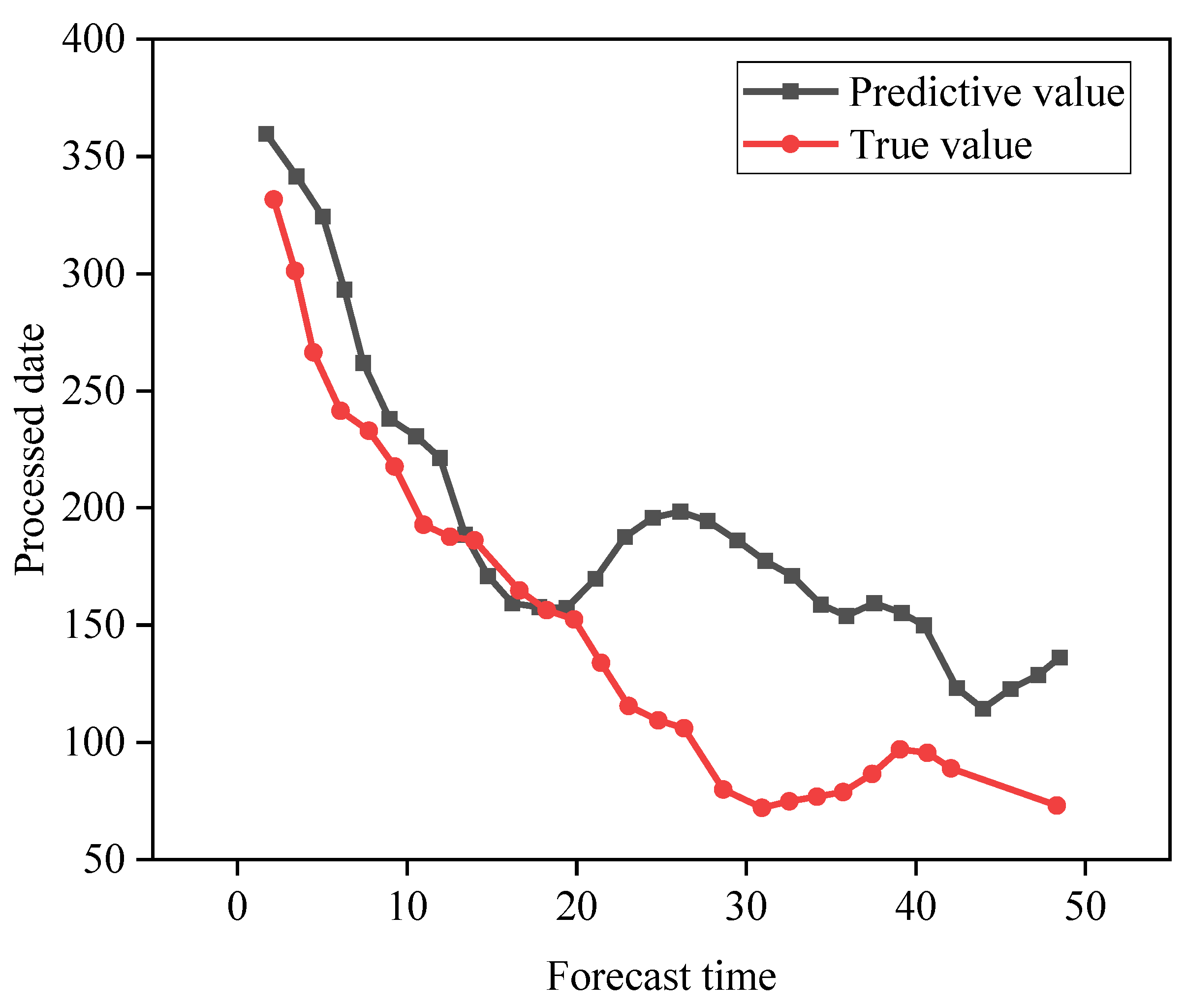
4.3. Carbon Emission Forecast Results
4.4. Policy Recommendations
- 1.
- Strengthen carbon market capacity building:
- 2.
- Strengthen corporate carbon asset management:
- 3.
- Properly assess the impact of new projects on carbon emissions:
- 4.
- Deploy large-scale carbon emission reduction technologies as early as possible:
5. Conclusions
Author Contributions
Funding
Institutional Review Board Statement
Informed Consent Statement
Data Availability Statement
Conflicts of Interest
References
- Xie, H.; Zheng, X.T.; Long, S.M. The characteristics and mechanism of the rapid and slow changes of the equatorial Pacific thermocline under the background of global warming. J. Ocean Univ. China (Nat. Sci. Ed.) 2021, 51, 12–19. [Google Scholar]
- Chen, Y.M.; Wang, Z.T.; Luo, H.L.; Qin, Y. Research progress in biofuel production from microalgae. Chem. Eng. Technol. 2021, 11, 10. [Google Scholar]
- Hong, J.K.; Li, Y.C.; Cai, W.G. Simulation of China’s carbon peak path from a multi-scenario perspective—By the RICE-LEAP model. Resour. Sci. 2021, 43, 639–651. [Google Scholar]
- Jalaee, S.A.; Shakibaei, A.; Akbarifard, H.; Horry, H.R.; GhasemiNejad, A.; Robati, F.N.; Derakhshani, R. A novel hybrid method by cuckoo optimization algorithm and artificial neural network to Forecast world’s CO2 emission. MethodsX 2021, 8, 101310. [Google Scholar] [CrossRef]
- Shivam, K.; Tzou, J.C.; Wu, S.C. A multi-objective predictive energy management strategy for residential grid-connected PV-battery hybrid systems by machine learning technique. Energy Convers. Manag. 2021, 237, 114103. [Google Scholar] [CrossRef]
- Kee, K.K.; Lim, Y.S.; Wong, J.; Chua, K.H. Impact of nonintrusive load monitoring on CO2 emissions in Malaysia. Bull. Electr. Eng. Inform. 2021, 10, 1803–1810. [Google Scholar] [CrossRef]
- Ning, L.; Pei, L.; Li, F. Forecast of China’s Carbon Emissions by ARIMA Method. Discret. Dyn. Nat. Soc. 2021, 21, 1–12. [Google Scholar] [CrossRef]
- Xie, B.C.; Tan, X.Y.; Zhang, S.; Wang, H. Decomposing CO2 emission changes in thermal power sector: A modified production-theoretical approach. J. Environ. Manag. 2021, 1, 111887. [Google Scholar] [CrossRef] [PubMed]
- Liu, X.; Meng, X.; Wang, X. Carbon Emissions Prediction of Jiangsu Province by Lasso-BP Neural Network Combined Model. IOP Conf. Ser. Earth Environ. Sci. 2021, 769, 17–22. [Google Scholar] [CrossRef]
- Acheampong, A.O.; Boateng, E.B. Modelling carbon emission intensity: Application of artificial neural network. J. Clean. Prod. 2019, 225, 833–856. [Google Scholar] [CrossRef]
- Wang, Z.; Zhao, Z.; Wang, C. Random forest analysis of factors affecting urban carbon emissions in cities within the Yangtze River Economic Belt. PLoS ONE 2021, 16, e0252337. [Google Scholar] [CrossRef]
- Yan, P.; Lu, H.; Chen, Y.; Li, Z.; Li, H. A stack-based set inversion model for smart water, carbon and ecological assessment in urban agglomerations. J. Clean. Prod. 2021, 319, 128665. [Google Scholar] [CrossRef]
- Huang, L.; Liu, S.; Yang, Z.; Xing, J.; Zhang, J.; Bian, J.; Li, S.; Sahu, S.K.; Wang, S.; Liu, T.-Y. Exploring Deep Learning for Air Pollutant Emission Estimation. Geosci. Model Dev. Discuss. 2021, 14, 4641–4654. [Google Scholar] [CrossRef]
- Rai, P.; Shukla, G.; Manohar, K.; Bhat, J.A.; Kumar, A.; Kumar, M.; Cabral-Pinto, M.; Chakravarty, S. Carbon storage of single tree and mixed tree dominant species stands in a reserve forest—Case study of the Eastern Sub-Himalayan Region of India. Land 2021, 10, 435. [Google Scholar] [CrossRef]
- Mohammed, S.; Gill, A.R.; Alsafadi, K.; Hijazi, O.; Yadav, K.K.; Hasanf, M.A.; Khan, A.H.; Islamf, S.; Cabral-Pintoh, M.S.M.; Harsanyi, E. An overview of greenhouse gases emissions in Hungary. J. Clean. Prod. 2021, 314, 127865. [Google Scholar] [CrossRef]
- Zhang, P.; Zhu, X.; He, Q.Y. Analysis on the temporal and spatial differentiation and balance pattern of ecosystem service supply and demand in the Yangtze River Economic Belt. Ecol. Sci. 2020, 39, 155–166. [Google Scholar]
- Huang, Z.X.; Wang, F.F.; Cao, W.Z. Analysis and prediction of factors affecting the level of ecological civilization in the Yangtze River Economic Zone—By VAR, GWR-BP neural network combined model. Econ. Geogr. 2020, 40, 199–209. [Google Scholar]
- Xia, L.L.; Yan, X.Y.; Cai, Z.C. Research progress and prospects of greenhouse gas emission reduction and organic carbon fixation in farmland soils in my country. J. Agric. Environ. Sci. 2020, 39, 178–185. [Google Scholar]
- Rubin, E.S.; Rao, A.B. A technical, economic, and environmental assessment of amine-based CO2 capture technology for power plant greenhouse gas control. Environ. Sci. Technol. 2019, 36, 4467–5542. [Google Scholar]
- Guo, Y.H.; Wang, F.Y.; You, H.Q. Effects of different carbon sources on the growth and active ingredient accumulation of Salvia miltiorrhiza and Tibetan Salvia miltiorrhiza hairy roots. Chin. J. Chin. Mater. Med. 2020, 45, 43–48. [Google Scholar]
- Lathika, N.; Rahaman, W.; Tarique, M.; Gandhi, N.; Kumar, A.; Thamban, M. Deep water circulation in the Arabian Sea during the last glacial cycle: Implications for paleo-redox condition, carbon sink and atmospheric CO2 variability. Quat. Sci. Rev. 2021, 257, 106853. [Google Scholar] [CrossRef]
- Mayes, R.T.; VanCleve, S.M.; Kehn, J.S.; Delashmitt, J.; Langley, J.T.; Lester, B.P.; Du, M.; Felker, L.K.; Delmau, L.H. Combination of DGA and LN Columns: A Versatile Option for Isotope Production and Purification at Oak Ridge National Laboratory. Solvent Extr. Ion. Exch. 2021, 39, 166–183. [Google Scholar] [CrossRef]
- Erdogan, S. Dynamic nexus between technological innovation and buildings Sector’s carbon emission in BRICS countries. J. Environ. Manag. 2021, 293, 112780. [Google Scholar] [CrossRef] [PubMed]
- Shan, A.; Fan, X.; Wu, C.; Zhang, X.; Fan, S. Quantitative Study on the Impact of Energy Consumption Based Dynamic Selfishness in MANETs. Sensors 2021, 21, 716. [Google Scholar] [CrossRef] [PubMed]
- Gu, S.Y.; Wu, Y.W. Input-output method to calculate and analyze China’s tourism carbon emissions. North Econ. Trade 2020, 423, 156–161. [Google Scholar]
- Cai, B.F.; Zhu, S.L.; Yu, S.M. Interpretation of “IPCC 2006 National Greenhouse Gas Inventory Guidelines 2019 Revised Edition”. Environ. Eng. 2019, 37, 4–14. [Google Scholar]
- Hu, Z.; Gong, X.; Liu, H. Analysis on the influencing factors and changing trend of household consumption carbon emission—Taking Shaanxi Province as an example. Ecol. Econ. 2020, 36, 28–34. [Google Scholar]
- Ehrlich, L.; Ledbetter, D.; Aczon, M.; Laksana, E.; Wetzel, R. 966: Continuous Risk of Desaturation Within the Next Hour Prediction Using a Recurrent Neural Network. Crit. Care Med. 2021, 49, 480. [Google Scholar] [CrossRef]
- Lin, K.; Zhao, Y.; Tian, L.; Zhao, C.; Zhang, M.; Zhou, T. Estimation of municipal solid waste amount by one-dimension convolutional neural network and long short-term memory with attention mechanism model: A case study of Shanghai. Sci. Total Environ. 2021, 791, 148088. [Google Scholar] [CrossRef]
- Xing, H. Research on the Multivariable Driving Factors of Carbon Emissions from Energy Consumption in the Yangtze River Economic Zone—By the Extended STIRPAT Model. Resour. Dev. Mark. 2020, 36, 4–10. [Google Scholar]
- Liu, Z.Q.; Xu, H.F.; Wang, C.Y. Research on the normalization method of scientific research scores by Sigmoid function. J. Xinxiang Univ. (Nat. Sci. Ed.) 2019, 36, 19–22. [Google Scholar]
- Zou, Y.B.; Lei, B.J.; Zang, Z.X. Automatic threshold selection method by the maximization of normalized mutual information. Acta Autom. Sin. 2019, 45, 1373–1385. [Google Scholar]
- Gonzaga, A.D.S.; Cordeiro, R. The similarity-aware relational division database operator with case studies in agriculture and genetics. Inf. Syst. 2019, 82, 71–87. [Google Scholar] [CrossRef]
- Chen, J. Several applications of Eviews software in unary linear regression model prediction. J. Foshan Univ. Sci. Technol. (Nat. Sci. Ed.) 2019, 37, 6–10. [Google Scholar]
- Tang, L.; Tian, Y.; Li, W.; Pardalos, P.M. Valley-loss regular simplex support vector machine for robust multiclass classification. Knowl.-Based Syst. 2021, 216, 106801. [Google Scholar] [CrossRef]
- Ding, S.; Sun, Y.; An, Y.; Jia, W. Multiple birth support vector machine by recurrent neural networks. Appl. Intell. 2020, 50, 2280–2292. [Google Scholar] [CrossRef]
- Liu, L.; Chu, M.; Gong, R.; Peng, Y. Nonparallel support vector machine with large margin distribution for pattern classification. Pattern Recognit. 2020, 106, 107374. [Google Scholar] [CrossRef]
- Chung, E.; Leung, W.T.; Pun, S.-M.; Zhang, Z. A multi-stage deep learning based algorithm for multiscale model reduction. J. Comput. Appl. Math. 2021, 394, 113506. [Google Scholar] [CrossRef]


| Indicator Definition | Representative Symbol | Index Quantification Unit |
|---|---|---|
| Total carbon emissions of provinces and cities in the Yangtze River Economic Belt | ZB1 | Ten thousand tons |
| Industry investment scale | ZB2 | CNY 100 million |
| Labor efficiency output | ZB3 | CNY 100 million /10,000 people |
| Carbon intensity | ZB4 | 10,000 tons/10,000 people |
| Openness to the outside world | ZB5 | % |
| Environmental protection | ZB6 | % |
| Guizhou Province | Jiangsu Province | ||
|---|---|---|---|
| Year | Carbon Emissions (×108 t) Year | Year | Carbon Emissions (×108 t) |
| 2000 | 1.845820987 | 2000 | 5.521659376 |
| 2001 | 1.50698462 | 2001 | 5.864446639 |
| 2002 | 1.622689431 | 2002 | 5.866892432 |
| 2003 | 2.079300127 | 2003 | 7.11895019 |
| 2004 | 2.422275528 | 2004 | 7.12083157 |
| 2005 | 2.765439067 | 2005 | 7.123089224 |
| 2006 | 2.767320446 | 2006 | 7.352053055 |
| 2007 | 2.767320446 | 2007 | 7.581581299 |
| 2008 | 2.656319082 | 2008 | 8.038003857 |
| 2009 | 3.226565072 | 2009 | 8.494990828 |
| 2010 | 3.455905178 | 2010 | 9.065236819 |
| 2011 | 3.45759842 | 2011 | 9.521471238 |
| 2012 | 3.800573821 | 2012 | 9.410469874 |
| 2013 | 4.257184516 | 2013 | 8.957621937 |
| 2014 | 4.259254033 | 2014 | 8.846244297 |
| 2015 | 4.261135412 | 2015 | 9.18903156 |
| 2016 | 4.3772165 | 2016 | 9.532195099 |
| 2017 | 4.492545036 | 2017 | 9.8751705 |
| 2018 | 4.492921311 | 2018 | 11.467946 |
| 2019 | 4.608249847 | 2019 | 13.51563896 |
| 2020 | 4.950848972 | 2020 | 14.54004986 |
Publisher’s Note: MDPI stays neutral with regard to jurisdictional claims in published maps and institutional affiliations. |
© 2021 by the authors. Licensee MDPI, Basel, Switzerland. This article is an open access article distributed under the terms and conditions of the Creative Commons Attribution (CC BY) license (https://creativecommons.org/licenses/by/4.0/).
Share and Cite
Huang, H.; Wu, X.; Cheng, X. The Prediction of Carbon Emission Information in Yangtze River Economic Zone by Deep Learning. Land 2021, 10, 1380. https://doi.org/10.3390/land10121380
Huang H, Wu X, Cheng X. The Prediction of Carbon Emission Information in Yangtze River Economic Zone by Deep Learning. Land. 2021; 10(12):1380. https://doi.org/10.3390/land10121380
Chicago/Turabian StyleHuang, Huafang, Xiaomao Wu, and Xianfu Cheng. 2021. "The Prediction of Carbon Emission Information in Yangtze River Economic Zone by Deep Learning" Land 10, no. 12: 1380. https://doi.org/10.3390/land10121380
APA StyleHuang, H., Wu, X., & Cheng, X. (2021). The Prediction of Carbon Emission Information in Yangtze River Economic Zone by Deep Learning. Land, 10(12), 1380. https://doi.org/10.3390/land10121380