Analysis of the Impact of Coastal Development and Utilization on the Ecological Environment of the Nearshore Area in the Liaohe River Estuary

Abstract

Based on an analysis of monitoring data from the Liaohe estuary, the distribution of inorganic nitrogen and active phosphate is related to the type of shoreline. The pollutant concentrations in the port area are 16% (inorganic nitrogen) and 59% (active phosphate) higher than those in the control area. The phytoplankton diversity index in the aquaculture area is 20% lower than in the mixed estuary area, which confirms the gradient effect of human disturbance. The constructed dual-mode distance effect model shows that, for a homogeneous shoreline, the goodness of fit is 40.1% in the non-estuary area, but radial basis function correction needs to be introduced for the estuary area. This study suggests that, in the port area, it is necessary to implement a combined policy consisting of ‘total nitrogen and phosphorus control + ecological compensation’, and artificial reefs should be built in the aquaculture area to maintain the number of benthic species.

1. Introduction

Due to the discontinuity between the ocean and land at the surface, the coastal zone has emerged as a geographic unit where land and ocean systems are interconnected and interwoven, becoming an area with the closest ties to human survival and development [1]. With the concentration of population and productivity in the coastal zone and rapid economic and social development, the intense development and utilization of coastal areas have significantly impacted the ecological environment of nearshore waters, making it a focal point of research across various fields [2,3,4,5,6].

The Liaohe Estuary is one of the seven major estuaries in China [7]. Many scholars have devoted themselves to studying the effects of land-sea interaction on estuarine ecology. Zhang Kexin et al. [8] found that the distribution characteristics of ¹³⁷Cs and ^239+240Pu in Liaohe estuary sediments were significantly disturbed by human activities. Wu [9] pointed out that the continuous input of terrestrial high-content nitrogen and low-content phosphorus was the main factor causing the increase of TN/TP in seawater of Liaodong Bay. According to their contribution, the main water pollution sources in this area were pollution sources caused by hydrological factors such as domestic sewage and industrial wastewater, hydrodynamic conditions, water-air interface material exchange and secondary conversion sources, and non-point sources generated by farmland surface runoff and transportation. The study of An [10] showed that the benthic community in the intertidal zone was sensitive to sediment particle size and organic matter content, and the construction of embankment would lead to local habitat fragmentation. Sun et al. [11] found that heavy metal pollution in the estuary of Yongdingxin River in Bohai Bay has obvious terrestrial characteristics through isotope tracing, which is comparable to the agricultural non-point source input in Liaohe Estuary. Wu et al. [12] pointed out that the concentration of polycyclic aromatic hydrocarbons (PAHs) in the Bohai Bay was positively correlated with human activities.

The synergistic effect of combined pollution sources in the estuary area has also attracted the attention of scholars. Fan et al. [13] confirmed that wastewater discharge from oil extraction areas can be converted into nitrogen and phosphorus pollution, resulting in eutrophication of water bodies and secondary pollution. Feng et al. [14] studied the non-point source pollution in the Haihe River Basin. The results showed that farmland runoff was the primary pollution source of nitrogen and phosphorus pollution in the Haihe River Basin, and urban domestic sewage was the secondary pollution source of non-point source pollution.

In terms of spatial heterogeneity of ecological response, Sun et al. [15] found that temperature and salinity were the main factors affecting the zooplankton community structure in the Yellow Sea. Naser [16] demonstrated that reclamation reduced the survival rate of macroinvertebrates by 58%. Wang et al. [17] pointed out that the embankment project of Chongming Dongtan in the Yangtze River estuary resulted in 12 species of zoobenthos. After the completion of the embankment, there were 6 species of zoobenthos, and only 2 species of the original 12 species of zoobenthos were retained. Jeppesen et al. [18] proposed a theoretical framework for zooplankton as a lake ecological indicator species.

The distance effect is widely used in various disciplines. Sutherland and Walsh [19] and Hanink [20] incorporated distance as an explanatory variable into the econometric model, and found that it is negatively correlated with the respondents’ willingness to pay for environmental goods (Willingness to Pay). Subsequently, the distance attenuation law has been verified in the research of watershed ecological management, lake environmental quality improvement, wetland ecological protection and other related fields. Pan [21] used the distance effect to study the changes of wetland plant community biomass, vegetation carbon storage, soil carbon storage, and ecosystem carbon storage. The results showed that according to the increase of the offshore distance of the sampling point, the aquatic plants showed different types of vegetation community zones at the level, and showed a banded distribution trend, and their biomass, carbon storage, and soil carbon storage showed a decreasing trend. Li and Zhang [22] studied the willingness to pay for the treatment of Enteromorpha prolifera in Qingdao based on the distance effect, and constructed a function model to measure whether there is a distance attenuation phenomenon between the distance of respondents from the seaside of Qingdao and their willingness to pay for the treatment of Enteromorpha prolifera. The results show that this ‘distance attenuation’ effect is obvious. Xu et al. [23] applied the distance effect theory to the study of rural residents’ willingness to participate in watershed ecological management. The results show that: different from the ‘distance attenuation’ law obtained in previous studies, the willingness of rural residents in the middle reaches of the Shiyang River Basin to participate in ecological management increases with the increase of distance from rivers and reservoirs, and the willingness of rural residents in the lower reaches to participate in ecological management increases with the increase of distance from reservoirs, showing a ‘distance enhancement’ law. In summary, the current research rarely applies the attenuation effect to the study of water quality changes. This paper intends to introduce the distance attenuation effect into the study of water quality changes, hoping to provide new ideas and scientific references for related research.

This paper examines the water quality and bio-ecological data of the nearshore sea area at the Liaohe River estuary, analyzing the impact of coastal development and utilization on the ecological environment through water quality monitoring data, biodiversity index, evenness index, and richness index. It also investigates the distance effect of water quality monitoring stations from the port, estuary, and aquaculture areas. Based on the analysis results, the paper proposes countermeasures and suggestions to provide decision-making references for relevant departments.

2. Materials and Methods

2.1. Research Area

2.1.1. Regional Survey

The study area is the coastal waters of Liaodong Bay, located between 40°28′12″ to 40°58′55″ N and 121°6′54″ to 122°11′52″ E. Three main rivers flow into the sea in this area. On the east side is the Daliao River, which includes the section where the Hun River and Taizi River merge from the Sanqiao River to the mouth of the Yingkou River. In the middle is the Liao River, one of China’s seven major rivers, originating from Guangtou Mountain in the Qilautu Mountain Range in the Chengde area of Hebei Province (elevation 1490 m). It flows through four provinces and regions—Hebei, Inner Mongolia, Jilin, and Liaoning—before entering the Bohai Sea (Also known as Shuangtai estuary) in Panjin City, Liaoning Province. On the west side is the Xiaoling River, which originates from Suiankala Mountain in Chaoyang County, Liaoning Province, flows through Chaoyang and Jinzhou, and enters the Bohai Sea from the southern suburb of Jinzhou. In recent years, with the rapid development of social economy and increasing human activities, the coastal zone of Liaohe Estuary is facing environmental problems such as the sharp decrease of sediment into the sea, the rapid increase of pollutants, the shrinking of wetland area and the gradual rise of sea level. These environmental problems make the contradiction between coastal zone development and protection increasingly prominent, and the bottleneck effect of environmental resources is also more prominent [8].

2.1.2. Population Situation

As an important economic belt in Liaoning Province, the Liaohe River estuary area has experienced a significant demographic transformation in the past 30 years. According to the data of ‘Liaoning Province Statistical Yearbook’ and ‘Panjin City Land and Space Master Plan (2021–2035)’, the permanent population of the whole region was about 780,000 in 1990, and increased to 1.24 million by 2020, with an average annual growth rate of 1.2%, which is higher than the average level of the whole province. The urbanization rate increased from 38% in 1990 to 67% in 2020, forming a bipolar agglomeration pattern with Panjin urban area (450,000 people) and Yingkou coastal industrial base (280,000 people) as the core. The proportion of employees in the oil extraction industry fell from 18% in 1990 to 9% in 2020, but the proportion of the employed population in the tertiary industry rose from 32% to 51%, reflecting the trend of industrial structure optimization. The size of the floating population increased from 87,000 in 2000 to 243,000 in 2020, accounting for 19.6% of the total population, of which the average annual growth rate of migrant workers in the coastal area reached 7.8%.

It is worth noting that the densely populated area is highly overlapped with coastal engineering: 34% of the permanent residents (about 420,000 people) of the whole area are concentrated within 5 km around Panjin Port, and the GDP output intensity per unit area in this area is 3.2 times that of the surrounding area. This coupling relationship of population-economy-development makes the coastal zone bear the dual pressure of human activities and ecological protection.

2.1.3. Climatic Factors and Their Evolution

The Liaohe River estuary area experiences a temperate, semi-humid, continental monsoon climate. According to the long-term observation data of the National Meteorological Science Data Center (2021), the average temperature in the area has significantly increased in the past 30 years (+0.31 °C/10 years). The warming rate in winter is 0.52 °C, and the increase in summer is 0.18 °C. The number of days with an extremely high temperature increased from an average of 1.2 days in 1990 to 5.7 days in 2020. The average annual precipitation amounts to 786 mm (coefficient of variation Cv = 0.21). In the past ten years, precipitation in the area has shown the characteristic of ‘wet-dry alternation’; in 2015, the precipitation exceeded the historical peak of 1000 mm, while that in 2019 amounted to only 623 mm, which was the lowest value in the same period. The proportion of precipitation occurring in the flood season (June–September) remained at 72–78%, but the concentration increased. The average annual evaporation amounted to 1823 mm (E601 pan), which was 15% higher than that in the 1980s. The dominant wind direction NE-ENE frequency accounted for 42% of the whole year. The maximum wind speed increased from 28.6 m/s in 1990 to 34.2 m/s in 2020, and the frequency of storm surge increased by 27%. The frequency of typhoons increased from an average of 1.2 times/decade in the 1990 s to 2.1 times/decade, and the intensity increased. The first freezing date of sea ice was advanced from mid-December to late November, and the duration was extended by about 15 days.

2.2. Survey Data Collection

In this study, water quality and bio-ecological data from the nearshore waters of the Liaohe estuary were collected during the fall of 2021 and the spring of 2022. The data primarily include measurements of pH, dissolved oxygen, chemical oxygen demand, salinity, inorganic nitrogen, nitrate, nitrite, reactive phosphate, oil, suspended solids, phytoplankton, zooplankton, and benthic fauna. The reason for selecting these two periods of data is that the two-year data cover a time span of about one year, which can initially reflect the short-term (seasonal to annual) environmental change trend. In addition, the autumn of 2021 and the spring of 2022 belong to different seasons, which may be affected by natural factors such as temperature, precipitation and runoff input. For example, in spring, the input of terrestrial pollutants may increase due to snowmelt, while in autumn, the exchange capacity of coastal waters may be changed due to typhoon or rainy season. This design helps to reveal the differences in the response of seasonal changes to the development and utilization of coastal zones.

The monitoring stations are shown in Figure 1, Figure 2 and Figure 3. In total, 46 monitoring stations were selected. Of these, #1–9 were concentrated near the estuary of the Daliao River; #10–17 were concentrated near the Shuangtaizi estuary (Liaohe estuary); #18–28 were concentrated in the vicinity of the reclamation area; #29–32 were on the outer edge of the study area, far from the coast; #33–36 were located at the Shuangtaizi estuary; #37–38 were located at the mouth of the Daliao River; #39–42 were located in the reclamation area; and #43–46 were located in the Panjin port area. The coordinate range is 40°50′24.85″ N at the north end, 40°28′17.04″ N at the south end, 122°05′28.86″ E at the east end, and 121°09′35.24″ E at the west end.

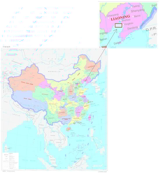
Figure 1. Location diagram of the study area. Note that the map of China comes from the http://bzdt.ch.mnr.gov.cn/ (accessed on 17 August 2025), standard map service system.

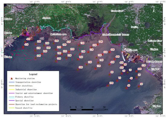
Figure 2. Distribution map of the utilization and monitoring stations along the Liaohe Estuary.

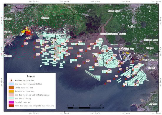
Figure 3. Map of the use type of the coastal waters of the Liaohe River Estuary.

2.2.1. Station Layout and Survey Time

A total of 31 water quality stations, 16 sediment stations, and 16 biological survey stations were set up. Two seasonal surveys were conducted in spring and autumn, respectively. The autumn survey time was from 28 August 2021–2 September 2021. The spring survey time was from 15 May 2022–18 May 2022. The sediment, biological survey and water quality survey were carried out simultaneously.

The data sampling and monitoring methods referred to the requirements of the ‘The specification for marine monitoring’ (GB17378-2007) [24] and ‘Specifications for oceanographic survey’ (GB12763-2007) [25]. Surface water samples were collected at depths of 0–5 m, on sunny days without wind, at 9 a.m. to 4 p.m., covering the operational time period.

2.2.2. Survey Items and Analysis Methods

The analysis method, detection limit and method basis of each investigation factor are shown in the Table 1, Table 2, Table 3 and Table 4.

Table 1. Analysis method of seawater survey project.

Number	Item	Analysis Method	Method Detection Limit	Method Standard
01	pH	pH meter method	/	‘The specification for marine monitoring’ (GB 17378.4-2007) [26]
02	Dissolved oxygen	Iodometry	/
03	Chemical oxygen demand	Alkaline potassium permanganate method	0.05 mg/L
04	Biochemical oxygen demand	Five-day training method	0.1 mg/L
05	Non-ionic ammonia	Non-ionic ammonia conversion method	/
06	Salinity	Seawater salinometer method	/
07	Ammonia	Hypobromite oxidation method	0.001 mg/L
08	Nitrate nitrogen	Cadmium column reduction method	0.002 mg/L
09	Nitrite nitrogen	Naphthalene ethylenediamine spectrophotometry	0.001 mg/L
10	Reactive phosphate	Phosphomolybdate blue spectrophotometric method	0.001 mg/L
11	Oil	Ultraviolet spec-trophotometry	0.0035 mg/L
12	Suspended matter	Gravimetric method	0.1 mg/L
13	Copper	Anodic stripping voltammetry	0.6 μg/L
14	Lead	Anodic stripping voltammetry	0.3 μg/L
15	Zinc	Anodic stripping voltammetry	1.2 μg/L
16	Mercury	Anodic stripping voltammetry	0.007 μg/L
17	Cadmium	Anodic stripping voltammetry	0.09 μg/L
18	Arsenic	Anodic stripping voltammetry	0.5 μg/L

Table 2. Sediment survey project analysis method.

Number	Item	Analysis Method	Method Detection Limit	Method Standard
01	Organic carbon	Potassium dichromate oxidation-reduction capacity method	0.20%	‘The specification for marine monitoring’ (GB 17378.4-2007) [26]
02	Sulfide	Methylene blue spectrophotometry	$0.3\times {10}^{-6}$
03	Oil	Ultraviolet spec-trophotometry	$3.0\times {10}^{-6}$
04	Copper	Flameless atomic absorption spectrophotometry	$0.5\times {10}^{-6}$
05	Lead	Flameless atomic absorption spectrophotometry	$1.0\times {10}^{-6}$
06	Cadmium	Flameless atomic absorption spectrophotometry	$0.04\times {10}^{-6}$
07	Zinc	Flame atomic absorption spectrophotometry	$6.0\times {10}^{-6}$
08	Total mercury	Atomic fluorometry	$0.002\times {10}^{-6}$
09	Arsenic	Atomic fluorometry	$0.06\times {10}^{-6}$
10	Chromium	Flameless atomic absorption spectrophotometry	$2.0\times {10}^{-6}$

Table 3. Analysis method of biological quality project.

Number	Item	Analysis Method	Method Detection Limit	Method Standard
01	Petroleum hydrocarbons	Fluorescence spectrophotometry	$0.2\times {10}^{-6}$	‘The specification for marine monitoring’ (GB 17378.4-2007) [26]
02	Copper	Non-flame atomic absorption spectrophotometry	$0.4\times {10}^{-6}$
03	Lead	Non-flame atomic absorption spectrophotometry	$0.04\times {10}^{-6}$
04	Cadmium	Non-flame atomic absorption spectrophotometry	$0.005\times {10}^{-6}$
05	Chromium	Non-flame atomic absorption spectrophotometry	$0.04\times {10}^{-6}$
06	Zinc	Non-flame atomic absorption spectrophotometry	$0.4\times {10}^{-6}$
07	Total mercury	Atomic fluorescence method	$0.002\times {10}^{-6}$
08	Arsenic	Atomic fluorescence method	$0.2\times {10}^{-6}$
09	$\alpha$-666	Gas chromatography	0.5 pg/g
10	$\beta$-666	Gas chromatography	0.7 pg/g
11	$\gamma$-666	Gas chromatography	0.3 pg/g
12	$\delta$-666	Gas chromatography	0.9 pg/g
13	$p,p^{\prime }$-DDE	Gas chromatography	0.5 pg/g
14	$o,p^{\prime }$-DDT	Gas chromatography	1.7 pg/g
15	$p,p^{\prime }$-DDD	Gas chromatography	0.8 pg/g
16	$p,p^{\prime }$-DDT	Gas chromatography	4.0 pg/g

Table 4. Analysis method of ecological survey project.

Number	Item	Analysis Method	Method Standard
01	Chlorophyll a	Spectrophotometry	‘The specification for marine monitoring’ (GB 17378.4-2007) [26]
02	Phytoplankton	Counting method
03	Zooplankton	Counting method
04	Macrobenthos	Counting method	‘Specifications for oceanographic survey’ (GB/T 12763.6-2007) [27]

2.3. Sampling Methods

Water quality sampling: water depth is less than 10 m, collecting surface seawater samples; when the water depth is greater than 10 m and less than 25 m, the surface and bottom seawater samples were collected. The water depth is greater than 25 m and less than 50 m, and the surface, water depth of 10 m and bottom seawater samples were collected. Oil only collected surface samples.

Sediment sampling: sediment samples were collected using a grab dredger, and the samples were placed in a clean polyethylene bag with a bamboo knife for heavy metal analysis; the samples were placed in brown glass sample bottles for the analysis of oil and organic carbon items. Sulfide samples were immediately fixed with zinc acetate after collection.

Phytoplankton: The phytoplankton survey method aligned with the ‘The specification for marine monitoring—Part 7: Ecological survey for offshore pollution and biological monitoring’ (GB17378.7-2007) [28] standard. A shallow-water type III (inner diameter 37 cm, net mouth area 0.1 m²) plankton net was used to collect phytoplankton from the bottom to the surface. The collected phytoplankton samples were loaded into the specimen bottle, and the samples were fixed and stored with formaldehyde solution. The amount of formaldehyde solution added was 5% of the sample volume. Phytoplankton samples were placed in storage bottles and numbered after standing, precipitation and concentration. The treated samples were identified and counted by individual counting method using optical microscope. According to the results of identification and counting, the number of cells in each species, the number of phytoplankton cells in each station and the average number of phytoplankton in the survey area were calculated. The number of individuals was expressed as N/m³.

Zooplankton: Zooplankton was dragged vertically from the bottom to the surface using shallow water type I net (large net, inner diameter of 50 cm, net mouth area of 0.20 m²) and type II net (medium net, inner diameter of 31.6 cm, net mouth area of 0.08 m²) according to the standard of ‘The specification for marine monitoring—Part 7: Ecological survey for offshore pollution and biological monitoring’ (GB 17378.7-2007) [28]. The obtained samples were fixed and stored with 5% formaldehyde. Zooplankton samples were analyzed by individual counting method and direct weighing method (wet weight). Individual counting: For the type I net, a value of 20% was applied; for the type II net, a value of 4% was applied; these were then summed to obtain the total count for both nets. The wet weight biomass of zooplankton was calculated in mg/m³ using type I net samples.

Macrobenthos: Macrobenthos were collected according to the standard of ‘Specifications for oceanographic survey-Part 6: Marine biological survey’ (GB/T 12763.6-2007) [27]. The macrobenthos were collected by 0.05 m² grab-type mud sampler four times per station. The sampling area was 0.2 m² and the sampling depth was 10–20 cm. The collected sediment samples were poured into a mesh of 0.5 mm benthic animal sample sieve, and the sediment was rinsed with water. All organisms were selected, placed in a specimen bottle, placed in a label, fixed with 5% formalin fixative, and the specimen was brought back to the laboratory for analysis (including species identification, weighing and calculation).

2.4. Quality Control During Sampling and Sample Analysis

Quality control and quality assurance measures are implemented in accordance with the requirements specified in the “Specifications for oceanographic survey” (GB/T 12763-2007) [27], “Marine Monitoring Specification” (GB17378-2007) [24] and “Specifications for oceanographic survey” (July 2000). The main quality assurance measures are as follows:

(1)

The monitoring unit is a qualified unit of measurement certification;

(2)

All the measuring instruments and equipment used are qualified by the national statutory measurement department and are within the validity period of the verification;

(3)

Sample collection, transportation and preservation, pretreatment and sample analysis were carried out in accordance with the requirements of “Specifications for oceanographic survey” (GB17378-2007) [24] and “Marine Monitoring Quality Assurance Manual” (2000);

(4)

According to the requirements of quality control methods, some monitoring items collect double parallel samples or prepare water quality standard samples at designated stations to analyze the precision and accuracy of monitoring data.

(5)

The reference materials used in the analysis of each project are certified products and within the validity period;

(6)

The data processing of each analysis project is carried out according to the relevant provisions of ‘Specifications for oceanographic survey’ (GB/T 12763-2007) [27] and ‘Specifications for oceanographic survey’ (GB17378-2007) [24].

2.5. Analysis Standards and Analysis Methods

2.5.1. Analysis of Water Quality, Sediment and Biological Quality

In December 2020, the Ministry of Ecology and Environment of the People’s Republic of China issued a series of national standards of ‘Specifications for oceanographic survey’ (HJ 442-2020) [29] in combination with China’s current marine environmental monitoring and evaluation requirements. According to the evaluation method of “Specifications for oceanographic survey” (HJ 442.10-2020) [30], seawater quality evaluation is carried out according to “Seawater Quality Standard” (GB3097-1997) [31], and the second-class seawater quality standard is uniformly adopted when calculating the exceeding rate of samples. The water quality category is represented by the ratio of the number of monitoring points to the total number of monitoring points in a certain category, that is, the sum of the number of monitoring points in a certain category accounts for the sum of all monitoring points. Sediment evaluation was performed according to ‘Marine sediment quality’ (GB18668-2002) [32], and the first-class sediment quality standard was used to calculate the over-standard rate of samples. The evaluation of marine biological quality was carried out according to the ‘Marine Biological Quality’ (GB18421-2001) [33], and the biological quality of fish was carried out according to the ‘Concise Procedure for Comprehensive Investigation of National Coastal Zone and Beach Resources’. In addition, the single factor pollution index analysis method was also used to analyze the water quality, sediment and biological quality indexes of the survey sea area (see Table 5, Table 6, Table 7 and Table 8).

Table 5. Seawater quality standard (unit: mg/L (except pH)).

Item	pH	COD	DO	Oil	Reactive Phosphate	Inorganic Nitrogen (in N)
Second standard	7.8∼8.5	≤3	>5	≤0.05	≤0.030	≤0.30
Item	Mercury	Arsenic	Copper	Lead	Zinc	Cadmium
Second standard	≤0.00020	≤0.030	≤0.010	≤0.005	≤0.050	≤0.005

Table 6. Marine sediment quality.

Item	Organic Carbon	Sulfide	Oil	Copper	Arsenic
First standard	$\le 2.0\times {10}^{-2}$	$\le 300.0\times {10}^{-6}$	$\le 500.0\times {10}^{-6}$	$\le 35.0\times {10}^{-6}$	$\le 20.0\times {10}^{-6}$
Item	Lead	Zinc	Cadmium	Mercury	Chromium
First standard	$\le 60.0\times {10}^{-6}$	$\le 150.0\times {10}^{-6}$	$\le 0.50\times {10}^{-6}$	$\le 0.20\times {10}^{-6}$	$\le 80.0\times {10}^{-6}$

Table 7. Marine biological quality standard (unit: mg/kg) (fresh weight).

Item	Petroleum Hydrocarbons	Total Mercury	Arsenic	Zinc	Cadmium	Lead	Copper	Chromium
First standard (bivalves)	≤15	≤0.05	≤1.0	≤20	≤0.2	≤0.1	≤10	≤0.5
First standard (fish)	≤20	≤0.3	≤1.0	≤40	≤0.6	≤2.0	≤20	≤0.5

Table 8. Classification of regional seawater quality status.

Water Quality Classification	Water Quality Status Level
First grade sea water	Outstanding
2nd class seawater	Good
Three types of seawater	Ordinary
Four types of seawater	Bad
Inferior four types of seawater	Too bad

2.5.2. Calculation Method of Single Factor Pollution Index

(1) The formula of single factor pollution index method is:

$$S_{i,j}={\displaystyle \frac{C_{i,j}}{C_{si}}}$$

(1)

In the formula: $S_{i,j}$ is the standard index of the analysis factor i at the jth sampling point; $C_{ij}$ is the mean value of all measured concentrations of the analysis factor i in the jth sampling; $C_{si}$ is the standard value of analysis factor i.

(2) The calculation formula of dissolved oxygen pollution index is:

When $D{O}_j\ge D{O}_s$, $S_{DO,j}={\displaystyle \frac{\left|D{O}_f-D{O}_j\right|}{\left|D{O}_j-D{O}_s\right|}}$;

When $D{O}_j<D{O}_s$, $S_{DO,j}=10-9{\displaystyle \frac{D{O}_j}{D{O}_s}}$.

In the formula: $S_{D}O,j$ is the standard index of dissolved oxygen at the sampling point j; $D{O}_f$ is the saturated dissolved oxygen concentration; $D{O}_j$ is the mean value of all measured concentrations of dissolved oxygen in water samples at sampling point j; $D{O}_s$ is the analysis standard of dissolved oxygen.

(3) According to the characteristics of pH, the calculation formula of pH pollution index is:

$$S_{pH,j}={\displaystyle \frac{\left|p{H}_j-(p{H}_{sd}+p{H}_{su})/2\right|}{\left|(p{H}_{su}-p{H}_{sd})/2\right|}}$$

(2)

In the formula: $S_{pH,j}$ is the standard index of pH at sampling point j; $p{H}_j$ is the mean value of the measured pH value of the water sample at the sampling point j; $p{H}_{sd}$ is the lower limit of the analytical standard; $p{H}_{su}$ is the upper limit value specified in the analysis standard.

2.5.3. Dominance Calculation Method

The concept of dominant species has two aspects. On the one hand, it occupies a wide range of ecological environment, can use high resources, has a wide range of adaptability, and has a high spatial frequency ($f_i$) in spatial distribution. On the other hand, it is characterized by a large number of individuals ($n_i$) and a high density $n_i/N$.

Let $f_i$ be the frequency of the ith species in each quadrat; $n_i$ is the number of individuals in the space of the first i species in the community; n is the sum of the number of individuals of all species in the community.

Combining the two aspects of the concept of dominant species, the calculation formula of dominant species dominance (Y) is obtained:

$$Y={\displaystyle \frac{n_i}{N}}\times f_i$$

(3)

2.5.4. Biodiversity Calculation Method

Shannon-Wiener index ($H^{\prime }$), Pielou’s evenness index (J) and Margalef index (d) were used to calculate the characteristics of plankton community. Among them, Shannon-Wiener index can reflect species diversity, Pielou’s evenness index can directly reflect the uniformity of individual number distribution in each community, Margalef index can reflect species richness, and its calculation formula [34,35,36,37,38] are as follows.

Shannon-Wiener index:

$$H^{\prime }=-\sum _{i=1}^S{P}_{i}ln{P}_i$$

(4)

Pielou’s evenness index:

$$J={\displaystyle \frac{H\prime }{lnS}}$$

(5)

Margalef index:

$$d={\displaystyle \frac{S-1}{lnN}}$$

(6)

In the above formula, N is the total number of individuals of all species, $P_i$ is the proportion of the number of individuals of the ith species to the total number of individuals at the monitoring station, and S is the total number of species.

2.6. Interpolation Simulation

In order to describe the impact of shoreline and sea area use on monitoring data, we use the interpolation analysis method in ArcGIS geostatistical analysis to interpolate the data around the monitoring points. The inorganic nitrogen index and the radial basis function (RBF) interpolation method are selected. The advantage of this method is that the algorithm is simple and can handle irregular or sparse data. The interpolation result has high accuracy and can effectively reduce the interpolation error [39]. For this research project, the monitoring point data is relatively irregular, which is more suitable for this interpolation method.

2.7. Spatial Data Information and Classification Mapping Basis

All the spatial data used in the study, including monitoring station coordinates, shoreline data and interpolation results, are based on CGCS2000 coordinate system and GK Zone 21 projection zone. The spatial resolutions of the covariates/driving factors used in this study were 12 m, respectively. The raster data used for spatial interpolation analysis (such as inorganic nitrogen distribution) in this study, and the output pixel size was set to 0.001475 degrees (data-based geographic coordinate system). In the study area (Liaohe estuary, about 41° N), the field size corresponding to this resolution is about 125 m × 164 m, and the interpolation simulation mapping is based on this resolution.

In this study, the natural breakpoint method was used to classify the concentration of each monitoring data and realize classification mapping. This method can maximize the difference between groups and minimize the difference within groups. In order to test the robustness of the conclusions, we use the natural breakpoint method and the quantile method to identify the hotspots. The results show that the main conclusions are not affected by the selection of classification methods.

3. Results

3.1. Sampling Results

3.1.1. Inshore Water Quality Monitoring Results

The statistical results of water quality monitoring in coastal waters are shown in Table 9 and Table 10.

Table 9. 2021 Statistical results of water quality monitoring.

Monitoring Stations	PH	Chemical Oxygen Demand mg/L	Biochemical Oxygen Demand mg/L	Salinity	Nitrate mg/L	Nitrite mg/L	Ammonia mg/L	Inorganic Nitrogen mg/L	Reactive Phosphate mg/L	Oil mg/L	Suspended Matter mg/L	N/P
1#	8.01	1.92	0.6	19.17	0.624	0.019	0.128	0.771	0.041	0.041	8.6	18.892
2#	7.97	1.67	0.8	22.19	0.337	0.179	0.157	0.673	0.021	0.024	7.5	31.745
3#	8.11	1.76	0.8	23.13	0.534	0.061	0.174	0.769	0.032	0.013	5.7	24.167
4#	8.07	1.56	0.4	23.83	0.756	0.06	0.057	0.872	0.011	0.004	2.9	78.586
5#	8.04	1.54	0.5	24.53	1.01	0.032	0.071	1.113	0.013	0.004	9.5	83.654
6#	8.16	1.61	0.4	26.51	0.776	0.058	0.291	1.125	0.011	0.004	10.7	106.085
7#	8.14	1.88	0.9	21.3	0.652	0.058	0.062	0.772	0.032	0.018	6.4	24.498
8#	8.01	1.47	0.9	24.15	0.712	0.072	0.043	0.827	0.028	0.006	15.3	29.539
9#	8.15	1.76	0.8	22.45	0.965	0.062	0.142	1.169	0.03	0.016	32.1	39.497
10#	8.05	2.8	0.8	21.04	1.17	0.05	0.11	1.33	0.03	0.04	99.3	42.91
11#	8.06	2.53	1	20.34	1.15	0.06	0.18	1.39	0.02	0.03	64.8	68.94
12#	8.14	1.95	0.9	21.88	1.09	0.04	0.05	1.19	0.02	0.02	43	49.59
13#	8.07	2.44	0.6	21.07	1.08	0.08	0.15	1.31	0.02	0.02	29.4	87.44
14#	7.94	2.83	0.9	18.47	1.12	0.04	0.21	1.36	0.04	0.02	43.6	30.89
15#	8.05	1.66	0.7	19.15	0.64	0.05	0.09	0.79	0.01	0.04	12.7	53.88
16#	8.1	2.43	0.9	19.84	0.49	0.04	0.08	0.61	0.03	0.02	17.9	18.6
17#	8.07	1.94	0.7	25.59	0.73	0.06	0.15	0.93	0.02	0.01	13.2	37.63
18#	7.98	1.64	0.8	20.17	0.77	0.07	0.08	0.91	0.01	0.02	20.5	93.57
19#	8.15	1.89	0.8	24.61	0.72	0.04	0.2	0.96	0.01	0.05	17.5	114.01
20#	8.08	1.62	1	20.87	0.87	0.05	0.1	1.02	0.01	0.02	27.8	81.72
21#	8.16	1.75	0.8	25.4	0.84	0.11	0.07	1.01	0.01	0.02	29.6	132.84
22#	8.02	1.8	0.9	21.53	0.78	0.08	0.1	0.95	0.01	0.01	16.3	89.51
23#	8.08	1.64	0.7	27.12	0.98	0.05	0.09	1.11	0.01	0.02	14.2	76.93
24#	8.03	1.5	0.8	27.27	0.96	0.04	0.06	1.06	0.01	0.04	17.2	116.39
25#	8.05	1.87	0.7	24.84	1.21	0.1	0.1	1.4	0.01	0.02	9.2	136.23
26#	8.1	1.35	0.8	21.58	1.07	0.22	0.14	1.43	0.01	0.04	15.3	195.63
27#	8.03	1.75	1	25.43	0.95	0.14	0.12	1.21	0.01	0.04	8.9	117.86
28#	7.99	1.67	0.9	26.58	0.89	0.09	0.11	1.09	0.01	0.05	23.6	154.79
29#	8.13	1.64	0.6	25.33	0.325	0.074	0.086	0.486	0.01	0.004	5.3	48.58
30#	8.02	1.4	0.8	25.81	0.37	0.08	0.02	0.47	0.02	0.02	7.3	28.23
31#	8.04	1.3	0.7	26.82	0.36	0.07	0.05	0.48	0.02	0.05	4.7	27.87
32#	7.91	1.52	0.9	27.9	0.41	0.1	0.13	0.64	0.02	0.03	15.7	40.83
33#	8.09	2.21	0.9	19.8	1.01	0.02	0.19	1.22	0.05	0.03	92.3	23.5
34#	8.04	2.22	0.9	20.76	0.97	0.02	0.28	1.27	0.04	0.03	101	30.88
35#	8.01	2.73	0.7	19.29	0.92	0.06	0.2	1.18	0.01	0.04	77.7	94.76
36#	8.02	2.51	0.9	20.42	1.04	0.09	0.12	1.24	0.01	0.04	68.3	84.84
37#	7.92	1.84	0.7	20.93	0.878	0.126	0.147	1.151	0.014	0.038	8	84.322
38#	7.93	1.94	0.8	20.2	0.9	0.164	0.173	1.237	0.012	0.044	4.8	101.393
39#	8.01	1.77	0.8	25.06	0.99	0.1	0.22	1.32	0.02	0.04	13.8	59.77
40#	7.92	1.52	1	26.81	0.5	0.16	0.14	0.8	0.01	0.04	39.8	55.42
41#	8.02	1.29	0.7	25.79	0.36	0.1	0.13	0.59	0.03	0.04	45.6	21.11
42#	7.98	2.68	0.8	25.2	0.88	0.09	0.24	1.22	0.02	0.05	20.3	72.39
43#	8.03	1.64	0.7	21.15	0.866	0.074	0.085	1.025	0.024	0.024	72.8	42.717
44#	8.06	1.97	0.9	20.16	1.03	0.058	0.064	1.152	0.036	0.019	52.4	32.092
45#	7.87	1.56	0.6	23.07	1.07	0.083	0.033	1.185	0.031	0.085	12	37.863
46#	7.93	1.64	1	23.23	0.735	0.202	0.105	1.042	0.023	0.015	17.8	44.53
Avg	8.0378	1.8611	0.7870	22.9950	0.8150	0.0800	0.1245	1.0187	0.0200	0.0282	27.8761	66.6765

Table 10. 2022 Statistical results of water quality monitoring.

Monitoring Stations	PH	Chemical Oxygen Demand mg/L	Biochemical Oxygen Demand mg/L	Salinity	Nitrate mg/L	Nitrite mg/L	Ammonia mg/L	Inorganic Nitrogen mg/L	Reactive Phosphate mg/L	Oil mg/L	Suspended Matter mg/L	N/P
1#	8.24	2.12	1.4	20.48	0.955	0.0062	0.204	1.16	0.00993	0.0365	12.7	116.8177
2#	8.19	2.4	1.6	22.42	0.92	0.0104	0.291	1.22	0.0024	0.0502	21.3	508.3333
3#	8.16	2	1.2	23.07	0.92	0.0075	0.284	1.21	0.0062	0.0272	43.1	195.1613
4#	8.32	1.99	1.4	23.61	0.813	0.0069	0.135	0.96	0.00156	0.0118	16.4	615.3846
5#	8.31	2.31	1.6	24.26	0.881	0.0076	0.185	1.07	0.00741	0.0206	27.7	144.3995
6#	8.26	2.24	1.6	25.21	0.646	0.0082	0.35	1	0.0149	0.0306	13.5	67.11409
7#	8.24	2.08	1.3	24.11	0.836	0.0072	0.191	1.03	0.00239	0.0171	12.1	430.9623
8#	8.23	2.45	1.8	23.92	0.904	0.0067	0.362	1.27	0.00212	0.0188	31	599.0566
9#	8.15	1.74	1.3	22.56	0.804	0.0074	0.296	1.11	0.00379	0.0222	66.2	292.876
10#	8.07	2.55	1.6	21.93	0.987	0.0053	0.29	1.27	0.012	0.106	72.8	105.8333
11#	8.03	1.68	1.3	21.48	0.755	0.0057	0.259	1.02	0.00462	0.0392	21.7	220.7792
12#	8.15	1.93	1.4	21.63	0.61	0.0062	0.104	0.72	0.00239	0.0276	25	301.2552
13#	8.09	1.98	1.4	21.49	0.39	0.0031	0.154	0.55	0.00128	0.049	33.4	429.6875
14#	8.17	1.87	1.4	20.72	1.02	0.0045	0.171	1.2	0.00062	0.0467	17	1935.484
15#	8.13	2.29	1.8	21.06	0.988	0.0047	0.199	1.19	0.00275	0.017	23.5	432.7273
16#	8.23	2.42	1.8	21.07	0.51	0.0066	0.162	0.68	0.0024	0.0035L	22.9	283.3333
17#	8.09	2.2	1.7	24.47	0.851	0.0064	0.226	1.08	0.00936	0.0474	29.7	115.3846
18#	8.12	1.96	1.6	24.79	0.654	0.0059	0.284	0.944	0.00267	0.0289	22.7	353.5581
19#	8.16	2.11	1.6	23.14	0.387	0.0053	0.181	0.573	0.00184	0.012	31.2	311.413
20#	8.19	1.93	1.4	20.68	0.332	0.0054	0.122	0.46	0.001	0.0168	24.7	460
21#	8.27	2.08	1.6	24.06	0.315	0.0042	0.13	0.449	0.00434	0.0453	22.4	103.4562
22#	8.14	1.8	1.4	23.46	0.792	0.0045	0.129	0.926	0.00323	0.0191	26	286.6873
23#	8.06	1.75	1.3	20.75	0.684	0.0063	0.1	0.79	0.00184	0.0226	19.2	429.3478
24#	8.23	2.09	1.5	21.47	0.188	0.0046	0.173	0.366	0.00156	0.0328	20.8	234.6154
25#	8.11	1.92	1.4	20.76	0.362	0.0039	0.228	0.594	0.00124	0.0171	25.2	479.0323
26#	8.17	1.61	1.3	20.54	0.344	0.0051	0.201	0.55	0.00184	0.0243	21.4	298.913
27#	8.17	1.71	1.4	21.43	0.18	0.0061	0.23	0.416	0.00239	0.0153	28.9	174.0586
28#	8.19	1.69	1.2	20.24	0.291	0.0057	0.298	0.595	0.00239	0.022	35.5	248.954
29#	8.18	1.77	1.4	25.03	0.731	0.0079	0.219	0.9579	0.00239	0.0191	31.4	400.795
30#	8.14	1.74	1.2	20.42	0.384	0.0055	0.219	0.61	0.00295	0.0189	32.5	206.7797
31#	8.08	1.93	1.6	25.24	0.836	0.0071	0.267	1.11	0.00323	0.0225	21.4	343.6533
32#	8.14	2.03	1.8	26.51	0.141	0.0081	0.155	0.304	0.00267	0.019	41.8	113.8577
33#	8.09	1.83	1.5	20.85	0.726	0.0049	0.258	0.99	0.00267	0.0402	41.6	370.7865
34#	8.11	1.96	1.6	20.34	0.75	0.0047	0.234	0.99	0.00434	0.0275	25.6	228.1106
35#	8.14	2.43	1.8	21.64	0.9	0.0055	0.111	1.02	0.00267	0.05	44.8	382.0225
36#	8.05	2.65	1.6	22.43	1.1	0.0059	0.091	1.2	0.00379	0.019	84.4	316.6227
37#	8.18	2.68	1.6	21.42	1.1	0.0122	0.26	1.37	0.00379	0.0239	32.1	361.4776
38#	8.23	2.48	1.5	21.26	0.873	0.0126	0.101	0.99	0.00128	0.0135	23.6	773.4375
39#	8.06	1.78	1.4	21.53	0.295	0.0071	0.241	0.543	0.00184	0.01	32.9	295.1087
40#	8.26	1.81	1.4	20.67	0.385	0.006	0.186	0.577	0.00062	0.0206	30.6	930.6452
41#	8.28	2	1.6	20.79	0.226	0.0043	0.118	0.348	0.00062	0.0066	28.6	561.2903
42#	8.25	2.19	2	20.37	0.222	0.0045	0.105	0.332	0.00062	0.0117	35.9	535.4839
43#	8.02	2.25	1.6	23.17	0.599	0.0092	0.138	0.75	0.00852	0.0085	72.5	88.02817
44#	8.19	2.26	1.3	21.86	0.985	0.0101	0.109	1.1	0.0133	0.0066	76.9	82.70677
45#	8.19	2.09	1.6	23.11	0.987	0.0065	0.1	1.09	0.0062	0.012	43.3	175.8065
46#	8.2	2.3	1.6	23.13	1.01	0.0056	0.107	1.12	0.001	0.0136	66.1	1120
Avg	8.167	2.067	1.509	22.273	0.665	0.006	0.195	0.865	0.004	0.02594	33.348	379.592

3.1.2. Phytoplankton Sampling Results

Phytoplankton: A total of 49 species of phytoplankton were identified in the autumn survey, including 42 species of diatoms, accounting for 85.72% of the species composition; there were 6 species of dinoflagellates, accounting for 12.24% of the species composition. One species was Chrysophyta, accounting for 2.04% of the species composition.

The dominant species of phytoplankton (dominance ≥ 0.02) from high to low were Coscinodiscus jonesianus, Leptocylindrus danicus, Paralia sulata, Chaetoceros curvisetus, Chaetoceros sp., Chaetoceros decipiens, Pseudo-nitzschia pungens, Ceratium tripos, Chaetoceros lorenzianus, Coscinodiscus granii, Skeletonema costatum, Chaetoceros affinis, the dominance was 0.18, 0.10, 0.08, 0.08, 0.08, 0.07, 0.05, 0.05, 0.04, 0.03, 0.03, 0.03 and 0.02, respectively. A total of 53 species of phytoplankton were identified in the spring survey, including 42 species of diatoms, accounting for 88.68% of the species composition. There were 6 species of dinoflagellates, accounting for 11.32% of the species composition. The dominant species of phytoplankton (dominance ≥ 0.02) from high to low were Noctiluca scintillans, Skeletonema costatum, Melosira sulcata, Chaetoceros lauderi, Coscinodiscus sp, Chaetoceros lauderi, and the dominance was 0.42, 0.15, 0.08, 0.06, 0.03, 0.03, 0.02, respectively.

Zooplankton: A total of 43 species of zooplankton in 8 categories were identified in the autumn survey. Among them, there were 1 species of Hymenoptera, 1 species of Amphipoda and 1 species of Lianchong, accounting for 2.33% of the species composition, respectively. There were 2 species of chaetognaths and 2 species of decapods, accounting for 4.65% of the species composition. There were 3 species of hydromedusae, accounting for 6.98% of the species composition. There were 18 species of copepods, accounting for 41.85% of the species composition. There were 15 species of planktonic larvae (insects), accounting for 34.88% of the species composition. The dominant species (classes) of shallow-water type I zooplankton (dominance ≥ 0.02) were Centropages dorsispinatus, Aidanosagitta crassa, Sagitta enflata, Paracalanus parvus, and Gastropoda larvae in descending order. Their dominance amounted to 0.39, 0.13, 0.09, 0.09, and 0.03, respectively. Paracalanus parvus, Oithona similis, Acartia, and Paracalanus crassirostris were the dominant species (classes) of shallow-water type II zooplankton, and their dominance values were 0.39, 0.22, 0.18, and 0.09, respectively. A total of 41 species of zooplankton in 9 categories were identified in the spring survey, including one species of tegument, one species of amphipoda, one species of krill, and one species of chaetognaths, accounting for 2.44% of the species composition. There were 2 species of decapods and 2 species of cladocera, accounting for 4.88% of the species composition, respectively. There were 7 species of hydromedusae, accounting for 17.07% of the species composition. There were 15 species of copepods, accounting for 36.59% of the species composition. There were 11 species of planktonic larvae (insects), accounting for 26.82% of the species composition. The dominant species (class) of shallow water type I net zooplankton (dominance ≥ 0.02) were Acartia, Podocoryne minima, Schmackeria poplesia and Oithona similis according to the dominance from high to low, and the dominance was 0.45, 0.16, 0.10 and 0.02, respectively. The dominant species (class) of shallow water type II net were in the order of A.hongi, A.pseudoannulata, Gastropod larvae and S.poplesia according to the dominance degree, and the dominance degrees were 0.68, 0.14, 0.03 and 0.03 respectively.

3.2. Distribution of Inorganic Nitrogen Influenced by Shoreline and Sea Use Types

3.2.1. Inorganic Nitrogen

In this study, the water quality indices included in the national standard (see Table 11) were selected, and the obtained histogram was compared with the standard. Through comparison, it is found that the overall water quality of Liaodong Bay is in good condition, only the inorganic nitrogen content index exceeds the standard seriously, and the other indexes are better.

Table 11. Seawater quality standard (GB3097-1997) [31].

Number	Item	Category I	Category II	Category III	Category IV
1	Chemical oxygen demand ≤ (COD)	2	3	4	5
2	Biochemical oxygen demand ≤ (BOD5)	1	3	4	5
3	Inorganic nitrogen ≤ (Calculated by N)	0.20	0.30	0.40	0.50
4	Reactive phosphate ≤ (Calculated by P)	0.015	0.030		0.045
5	Oil ≤	0.05		0.30	0.50

Note: The content of this table is extracted from the ‘National Standard of the People’s Republic of China Sea Water Quality Standard’ (GB3097-1997) [31].

In terms of inorganic nitrogen content, this index in the coastal waters of Liaodong Bay exceeds the standard seriously, see Table 12. The sources of inorganic nitrogen pollution are complex, including not only the main ways of non-point source pollution such as agricultural breeding industry and urban and rural domestic sewage discharge in the catchment area of the whole basin, but also the causes of point source discharge such as industrial production and sewage treatment plant. Along with economic and social development and changes in urban and rural production and lifestyles, it will inevitably lead to dynamic changes in nitrogen emissions [40]. The rivers entering the sea in Liaodong Bay are mainly Liaohe River, Daliao River and Xiaoling River. Among them, the Panjin area where the Liaohe River flows through is the main oil field distribution area, which is the largest heavy oil and high pour point oil production base in China. Petroleum industry activities, including exploration, mining, processing and refining, will produce wastewater and waste containing various chemicals. These substances may include ammonia, nitrates, nitrites, and other forms of nitrogen compounds, all of which may be converted into inorganic nitrogen in the environment, causing huge pollution to ecological environments such as the ocean [13].

Table 12. The inorganic nitrogen content of the seawater at the monitoring station exceeded the standard.

Year	Average Value (mg/L)	Percentage of Sites Exceeding Class 1 Seawater Standard	Percentage of Sites Exceeding Class 2 Seawater Standard	Percentage of Sites Exceeding Class 3 Seawater Standard	Percentage of More Than 4 Types of Seawater Standard Sites
2021	1.019	100.0%	100.0%	100.0%	93.5%
2022	0.865	100.0%	100.0%	91.3%	84.8%

The monitoring results of inorganic nitrogen in the coastal waters of Liaodong Bay show that the data in 2021 and 2022 reflect that the inorganic nitrogen content in Liaodong Bay exceeds the standard seriously, and the exceeding rate of class 1 and class 2 water quality is 100%. The over-standard rate of the three types of water quality in 2021 was 100%, and over-standardthe rate in 2022 was 91.3%. The over-standard rate of the four types of water quality in 2021 was 93.5%, and the over-standard rate in 2022 was 84.8%. From the distribution map of 2022 (see Figure 4), it has obvious regional characteristics, that is, the inorganic nitrogen content in the sea area near Panjin Port is significantly higher than that in the west side of Shuangtai Estuary. There are many reasons for this. First, the port operation and ship activities of Panjin Port are related to the increase of inorganic nitrogen concentration in water. Panjin Port is an important hub port, and high-frequency berthing of ships will bring direct emission of nitrogen-containing pollutants. For example, the process of exhaust gas deposition, bilge sewage discharge and cargo residue dissolution produced by ship fuel combustion will release inorganic nitrogen to the water body. The second is the difference in hydrodynamic conditions. Panjin Port may lead to limited water exchange rate due to terrain shielding or artificial breakwater construction, resulting in the accumulation of inorganic nitrogen, while the west side of Shuangtai Estuary is in a strong tidal current or open water environment, which is conducive to the rapid diffusion and dilution of pollutants. The third is the potential ecological chain amplification mechanism. High concentration of inorganic nitrogen is easy to induce algae fulminant proliferation, and the decomposition of organic matter after death will reversely increase the nitrogen salt content in water, forming a positive feedback cycle. This process is particularly significant in the relatively closed port area.

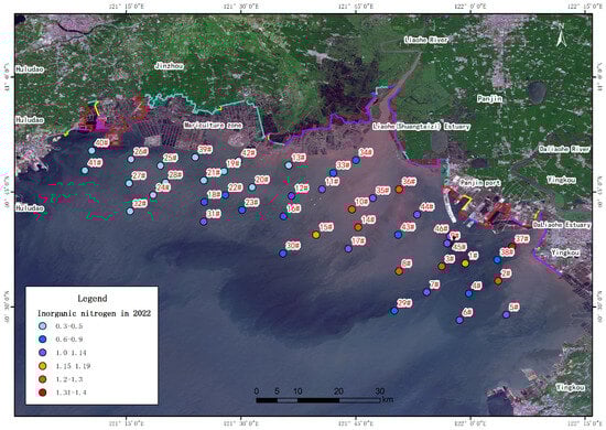
Figure 4. Distribution map of inorganic nitrogen content at monitoring sites in 2022.

3.2.2. Active Phosphate

In 2021, the monitoring station recorded elevated levels of active phosphate (see Figure 5) in the Panjin Harbor and Liaohe estuary sea areas, while the aquaculture area on the west side of Liaohe estuary exhibited generally low values for this indicator. In densely populated harbor regions, domestic sewage, which often contains high concentrations of phosphate, is produced. If sewage treatment facilities are inadequate or ineffective [14], these phosphates can enter harbor waters, thereby increasing the active phosphate content. Additionally, the rise in active phosphate levels at the mouths of some large rivers can be attributed to the transport of land-based substances rich in phosphate by these rivers [11,12]. This influx of phosphates significantly influences the distribution of reactive phosphate in nearshore waters [41].

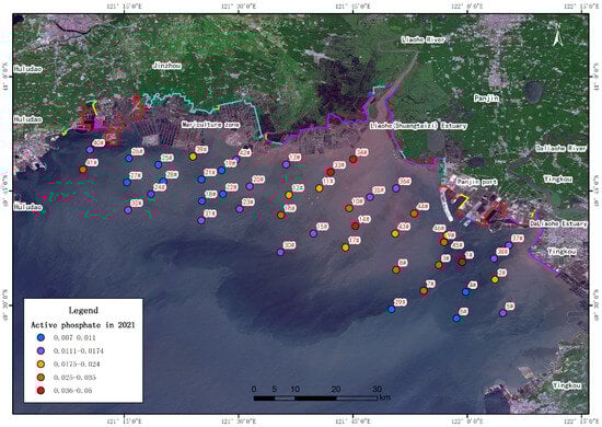
Figure 5. Distribution of active phosphate content at monitoring sites in 2021.

3.3. Clustering and Interpolation Simulations

3.3.1. Cluster Analysis

Given that the monitoring data for inorganic nitrogen and reactive phosphate were clearly influenced by the type of shoreline and sea use, we conducted a cluster analysis of water quality data from all 46 monitoring stations using the SPSS software (13.0) [42]. This analytical method was employed to identify data with similar characteristics. The Table 13 presents the results of the cluster analysis. Through repeated testing, it was found that division into six categories yielded the best distinctiveness.

Table 13. Cluster analysis results.

Case	6 Clusters	Case	6 Clusters	Case	6 Clusters
1	1	17	3	33	5
2	2	18	3	34	5
3	3	19	3	35	5
4	3	20	3	36	5
5	3	21	3	37	3
6	4	22	3	38	3
7	3	23	3	39	3
8	3	24	3	40	2
9	3	25	3	41	2
10	5	26	6	42	3
11	5	27	3	43	3
12	3	28	3	44	3
13	3	29	2	45	3
14	5	30	2	46	6
15	3	31	2
16	3	32	2

We use GIS software (ArcMap 10.7) to label the results of cluster analysis on the map. It can be clearly seen from Figure 6 that the data size of 34#, 33#, 11#, 36#, 35#, 10# and 14# monitoring stations in Shuangtai Estuary (Liaohe Estuary) is relatively close.

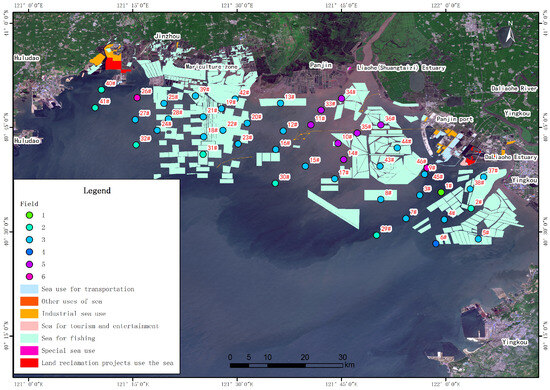
Figure 6. Cluster analysis of monitoring data in 2021.

In the periphery of the coast, there is no similar data size of 29#, 30#, 32#, 40#, 41# and other sea area use types shown in the map, while the monitoring stations in the open aquaculture area on the west side of the Shuangtai estuary, such as 42#, 39#, 20#, 22#, 25#, 28#, 24# and other data sizes are relatively close. The characteristics of this open aquaculture area also exist in some aquaculture areas on the east side of Shuangtai Estuary, indicating that the water quality characteristics of the open aquaculture area are relatively consistent. In addition, two major reclamation areas in the study area, such as Panjin port area at point 9# and Jinzhou port logistics center area at point 26#, also showed consistent analysis results. This reflects that the use of shoreline has a certain influence on the monitoring data.

3.3.2. Interpolation Simulation Results

The interpolation results (see Figure 7, Figure 8 and Figure 9) indicate that the distribution of data reflects the influence of shoreline and sea use types on the nearshore area. Specifically, the interpolation results for the Panjin port area on the east side of the Liaohe estuary show higher values. Additionally, there is an extensive range of medium-value areas within the Liaohe estuary, which aligns closely with the distribution trend of measured data from the monitoring stations. This suggests a correlation between water quality conditions and the utilization of shoreline and sea areas.

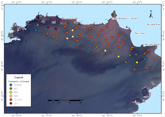
Figure 7. The original data map of inorganic nitrogen concentration at monitoring points.

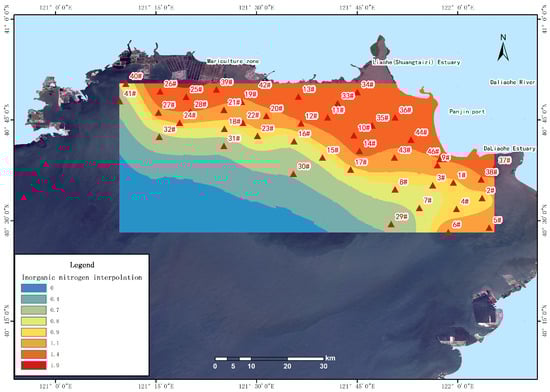
Figure 8. Inorganic nitrogen interpolation analysis diagram in the study area.

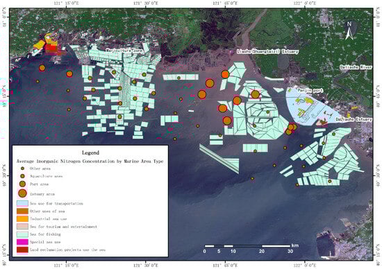
Figure 9. The average concentration of inorganic nitrogen in different types of sea area.

3.4. Analysis of Phytoplankton Indexes

Shoreline development and utilization, along with offshore sea use, are primary factors influencing changes in offshore ecosystems. Marine phytoplankton serves as a crucial indicator of the health of marine ecosystems. Phytoplankton comprises photosynthetic autotrophic organisms that spend part or all of their life cycle floating in oceans, lakes, ponds, or rivers [43]. The species composition, community structure, and dynamics of phytoplankton directly or indirectly influence ocean productivity. By altering indicators such as ocean carbon flux, phytoplankton can subsequently impact global climate and human survival [44,45]. In our study, we examined the biodiversity, abundance, and evenness of phytoplankton at various monitoring stations. The results indicated that these indicator values were significantly affected by the type of shoreline and sea area use, exhibiting variations in magnitude.

3.4.1. The Characteristic Values of Each Index of Phytoplankton

The phytoplankton diversity index is an indicator of the diversity of its community. It is generally considered to be normal when it is greater than 1, and may be disturbed by other environmental factors when it is less than 1. The evenness is the ratio of the actual diversity index to the theoretical maximum diversity index. In practical application, when the evenness is greater than 0.3, it indicates that the diversity of phytoplankton in the sea area is better. At present, the diversity index less than 1 and the evenness less than 0.3 are often used as the criteria for poor biodiversity for comprehensive evaluation [46].

It can be seen from Table 14 that the average diversity of the study area was 3.52, and the average evenness was 0.81. The diversity and evenness indexes were good, indicating that the species composition and ecological types of phytoplankton in the offshore area of Liaodong Bay were abundant, and the community structure showed a variety of structural complex characteristics [47].

Table 14. The number of phytoplankton species and the characteristic values of each index in the coastal waters of the Liaohe River Estuary in 2021.

Monitoring Stations	Diversity	Uniformity	Richness
1	3.17	0.69	3.63
2	3.85	0.85	3.66
3	3.92	0.83	4.3
5	3.92	0.84	3.38
6	3.95	0.84	3.99
8	3.22	0.76	2.72
11	3.65	0.86	3.01
13	3.39	0.8	2.93
17	3.37	0.78	2.92
21	3.63	0.81	3.78
23	3.24	0.75	3.18
25	3.32	0.81	2.49
26	3.68	0.85	3.3
30	3.75	0.87	3.67
31	3.44	0.77	3.91
32	3.78	0.86	3.66
34	3.64	0.84	3.18
35	3.39	0.8	2.93
37	3.86	0.87	3.27
40	3.52	0.8	3.8
41	3.22	0.75	3.16
42	3.16	0.83	2.62
44	3.22	0.81	2.54
46	3.22	0.77	3.17
Max	3.95	0.87	4.3
Min	3.16	0.69	2.49
Avg	3.52	0.81	3.3

3.4.2. Diversity Index Analysis

The diversity index measured from the monitoring data in the study area ranged from 3.16 to 3.95. Excluding stations with no monitoring values, the highest index value was observed at station 6#, located at the mouth of the Daliao River. The lowest value was recorded at site 42#, situated on the west side of the Liaohe estuary in the aquaculture area. Additionally, sites 1# and 46#, which are closer to the harbor, also exhibited very low monitoring values. According to Zhou [48], harbor waters can be disturbed by dredging projects, leading to the disappearance of phytoplankton species [35]. As illustrated in the Figure 10, areas with high phytoplankton diversity values are primarily distributed in the region circled in yellow, with the west side at the mouth of the Xiaoling River, the center at the mouth of the Liao River, and the east side at the mouth of the Daliao River. The phytoplankton diversity values in the Daliao River estuary exceeded 3.85, while the diversity values in the other two areas generally ranged between 3.6 and 3.8. The Daliao River has a total length of 94 km and a watershed area of 1926 square kilometers. Including the watershed areas of its tributaries, the Hun River and the Taizi River, the total watershed area of the Daliao River reaches 27,326 square kilometers. Due to the high concentration of nutrient salts, phytoplankton diversity is typically higher in the shallow water or inner sections of a river’s estuary compared to areas outside the estuary or in the bay. This has been identified as a distinctive feature in numerous studies of estuaries [49,50,51].

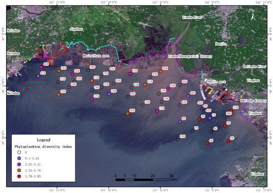
Figure 10. Phytoplankton diversity index distribution map of monitoring sites in 2021.

3.4.3. Uniformity Index Analysis

As shown in Figure 11, The homogeneity index measured from monitoring data in the study area ranged from 0.69 to 0.87, indicating a generally higher homogeneity of phytoplankton near the estuaries of the Liao, Daliao, and Xiaoling Rivers. This can be attributed to several factors:

Figure 11. Phytoplankton evenness index distribution of monitoring sites in 2021.

First, the input of nutrient salts, particularly nitrogen and phosphorus, carried by the rivers may create favorable conditions in the estuarine areas, promoting the growth of a diverse range of phytoplankton species and thereby enhancing species diversity and evenness.

Second, the mixing of fresh and brackish water as rivers enter the sea may lead to the formation of a variety of ecological niches suitable for different phytoplankton species, contributing to increased community evenness.

Third, the dynamics of water currents may facilitate a more uniform distribution of phytoplankton throughout the water column, reducing localized aggregation and thus enhancing evenness.

3.4.4. Richness Index Analysis

From the distribution map of the richness index in the study area (Figure 12), it is observed that the richness index at the estuary of the Daliao River and the adjacent area of Panjin Harbor is lower than that of the open sea. Similarly, the richness index at the Liao River estuary also exhibits a declining trend, but at monitoring points further from the estuary, a higher richness index is noted. Overall, the richness index tends to increase with greater distance from the estuary and the shoreline. This variation may be attributed to several factors:

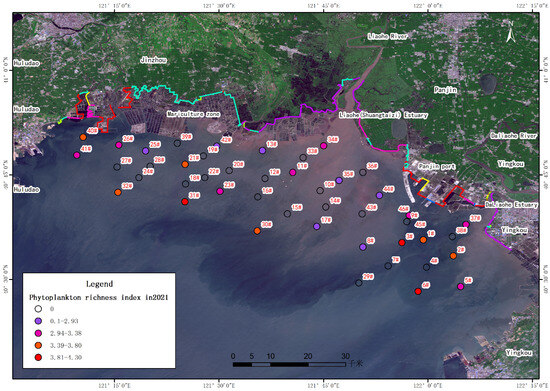
Figure 12. Phytoplankton richness index distribution map of monitoring sites in 2021.

First, the mixing of freshwater and seawater at river estuaries creates a transitional zone where the sudden change in salinity can exert stress on phytoplankton, as not all species can adapt to such drastic changes. In contrast, areas further from the shore offer a more stable water environment, reducing stress on phytoplankton.

Second, nutrient dilution occurs as nutrient salts carried by rivers mix with seawater at the estuary, leading to a decrease in nutrient concentration, which can limit phytoplankton growth. In regions farther from the estuary, nutrient salts (such as nitrogen and phosphorus) have been sufficiently mixed and diluted to concentrations conducive to phytoplankton absorption and utilization. This “nutrient salt balance” supports the growth and reproduction of phytoplankton.

Third, the dynamics of currents in the estuary area are complex and variable. Strong currents and waves can physically damage phytoplankton, whereas in areas away from the estuary, the absence of strong currents and waves, along with ocean circulation and interactions between different water masses, can provide nutrients favorable for phytoplankton growth.

3.5. Analysis of Zooplankton Indexes

Zooplankton is a crucial component of the marine food chain and plays a key role in the biological pumping process [15]. It serves an important regulatory function in marine ecosystems, where dynamic changes in its abundance, distribution, species composition, and community structure influence the rhythms, scales, and outcomes of primary productivity, see Table 15. These changes can directly reflect the health of marine ecosystems [18], the quality of the water environment, and the status of material cycling and energy flow [52,53,54].

Table 15. Index characteristic values of zooplankton in the coastal waters of the Liaohe River Estuary in 2021.

Station Number	Shallow Water Type I Mesh (The Inner Diameter is 50 cm, and the Net Mouth Area is 0.20 m2)			Shallow Water Type II Mesh (The Inner Diameter is 31.6 cm, and the Net Mouth Area is 0.08 m2)
	Diversity Index (${\mathit{H}}^{\prime }$)	Uniformity ($\mathit{J}$)	Richness ($\mathit{d}$)	Diversity Index (${\mathit{H}}^{\prime }$)	Uniformity ($\mathit{J}$)	Richness ($\mathit{d}$)
1	1.93	0.51	1.49	2.23	0.6	0.91
2	1.88	0.54	1.12	2.15	0.56	0.98
3	1.81	0.48	1.47	2.3	0.62	0.91
5	2	0.54	1.39	2.2	0.58	1.01
6	2.59	0.61	2.21	2.39	0.59	1.21
8	1.98	0.55	1.44	2.18	0.55	1.15
11	1.81	0.5	1.19	1.77	0.49	0.81
13	2.36	0.75	0.89	2.35	0.68	0.77
17	2.14	0.58	1.39	2.2	0.56	1.04
21	2	0.53	1.56	2.35	0.58	1.17
23	2.31	0.59	1.7	2.3	0.58	1.11
25	2.61	0.73	1.24	1.91	0.55	0.7
26	2.39	0.65	1.39	2.02	0.56	0.8
30	2.05	0.54	1.56	2.32	0.57	1.17
31	2.01	0.53	1.55	2.7	0.65	1.25
32	2.47	0.6	1.94	2.19	0.54	1.19
34	2.5	0.75	0.96	1.98	0.62	0.58
35	1.85	0.52	1.2	1.63	0.47	0.71
37	2.14	0.55	1.51	2.04	0.57	0.81
40	2.58	0.64	1.85	2.16	0.58	0.89
41	2.12	0.56	1.59	2.39	0.6	1.14
42	2.4	0.76	0.98	2.06	0.62	0.64
44	2.67	0.8	0.93	1.34	0.45	0.47
46	1.94	0.52	1.37	2.31	0.64	0.79
Max	2.67	0.8	2.21	2.7	0.68	1.25
Min	1.81	0.48	0.89	1.34	0.45	0.47
Avg	2.19	0.6	1.41	2.15	0.58	0.93

3.5.1. Diversity Index and Evenness Index Analysis

The diversity index of zooplankton species in the nearshore waters of the Liaohe estuary ranged from 1.81 to 2.67, with a mean value of 2.19. The highest value was recorded at station 44, followed by 2.61 at station 25 and 2.59 at station 6. The lowest values were observed at stations 3 and 11. The distribution trend of species evenness mirrored that of the diversity index, ranging from 0.48 to 0.8, with a mean value of 0.6. The highest evenness was found at station 44, followed by 0.76 at station 42, and 0.75 at stations 34 and 13. The lowest evenness was recorded at station 3, followed by 0.5 at station 11.

Regarding the diversity index, the range of 1.81 to 2.67 suggests a good level of zooplankton diversity in the area. As a typical deltaic estuary, the Liaohe Estuary features a unique ecological environment, including a well-developed intertidal zone and abundant wetland resources. These characteristics provide habitats for a wide range of organisms, thereby supporting high biodiversity levels. In terms of evenness, which indicates the degree of uniformity in species distribution within a community, values typically range from 0 to 1, with higher values signifying a more uniform species distribution. The zooplankton evenness index in the nearshore waters of the Liaohe estuary ranged from 0.48 to 0.8, with an average value of 0.6. This suggests that zooplankton evenness in the study area is moderate to above average. However, to more accurately assess the state of evenness, future studies should compare these findings with historical data from the area or data from similar ecosystems.

3.5.2. Richness Index Analysis

Using shallow water type I net samples as an example, the zooplankton abundance index in the nearshore waters of the Liaohe estuary ranged from 0.89 to 2.21, with an average value of 1.41. The highest abundance was recorded at station 6, while the lowest was at station 13. Overall, the nearshore waters of the Liaohe Estuary exhibit a high number of zooplankton and rich species diversity. However, there are significant variations in zooplankton abundance among the monitoring stations, with an uneven distribution pattern. For instance, the abundance at station 25, which is at a similar latitude to station 13, differs by an order of magnitude, while the abundance at station 40, also at a similar latitude, differs by four orders of magnitude (see Figure 13).

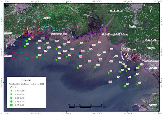
Figure 13. Distribution of zooplankton (shallow water type I reticulum) richness index in 2021.

The monitoring data and graphs indicate that zooplankton abundance is higher near the mouths of the Daliao River (Panjin Harbor) and the Xiaoling River, whereas it is lower at the mouth of the Liaohe River. This pattern is similar to the distribution of phytoplankton abundance shown in Figure 13, reflecting a strong correlation between the distributions of zooplankton and phytoplankton. Additionally, zooplankton abundance tends to increase from nearshore to offshore areas, with higher values recorded at stations 32, 31, 30, and 6, which are located farther from the shore. Numerous studies have demonstrated that seawater salinity influences the distribution of zooplankton [55,56,57,58].

3.6. Analysis of Benthic Indices

Benthic animals primarily consist of aquatic species that reside underwater for all or part of their life cycle and are unable to pass through a sieve with a 0.5 mm aperture. These organisms live on or are attached to the substrate of water bodies and sediments [59]. They are a common and vital component of the intertidal zone, playing a significant role in material decomposition and nutrient cycling within ecosystems. The macrobenthos of the intertidal zone predominantly includes coelenterates, nematodes, annelids, mollusks, crustaceans, and aquatic insects [10].

Due to their long life cycles, limited mobility, difficulty in migrating, and sensitivity to environmental changes, benthic animals can provide accurate reflections of the extent to which a region’s habitat has been impacted by external influences [16,60]. Consequently, indices of benthic fauna are commonly used as primary indicators for evaluating the water environment in estuaries and coastal areas.

The diversity index of zoobenthos in the coastal waters of Liaodong Bay ranged from 0.79 to 1.49, with an average of 1.15 (Table 16). As shown in Figure 14, the highest value was recorded at monitoring station 17#, while the lowest was at station 26#. The evenness index ranged from 0.25 to 0.43, with a mean value of 0.35. The highest evenness was observed at station 37#, and the lowest at station 26#. Previous studies have indicated that dike projects can disturb estuarine salt marsh wetland habitats by altering tidal dynamics, impeding tidal water circulation, and restricting nutrient flow, which can lead to a decline in habitat quality and a reduction in benthic fauna populations [17].

Table 16. Characteristic values of benthic index in the coastal waters of the Liaohe River Estuary in 2021.

Station Number	Diversity Index (${\mathit{H}}^{\prime }$)	Uniformity (J)	Richness (d)
1	1.19	0.33	1
2	1.31	0.39	0.82
3	1.41	0.41	0.91
5	1.08	0.31	0.91
6	1.03	0.32	0.73
8	0.91	0.3	0.63
11	1.22	0.37	0.82
13	0.9	0.26	0.91
17	1.49	0.42	1
21	1	0.32	0.73
23	1.25	0.38	0.82
25	1.3	0.38	0.91
26	0.79	0.25	0.73
30	1.02	0.31	0.82
31	1.17	0.37	0.73
32	1.06	0.32	0.82
34	0.97	0.28	0.91
35	1.09	0.34	0.73
37	1.36	0.43	0.73
40	1.16	0.35	0.82
41	1.41	0.41	0.91
42	0.86	0.27	0.73
44	1.4	0.42	0.82
46	1.16	0.35	0.82
Max	1.49	0.43	1
Min	0.79	0.25	0.63
Avg	1.15	0.35	0.82

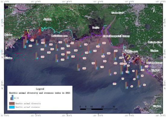
Figure 14. Map of the benthic animal diversity and evenness index in 2021.

In this study area, the dikes of Panjin Harbor are particularly prominent. According to the Environmental Impact Report of the Panjin Harbor Master Plan (Revised in 2016), the ecological community structure of the Panjin Harbor sea area, along with the surrounding sea areas of the Daliao River and Shuangtaizi Estuary, facilitates immediate biological information and species exchange, contributing to a certain degree of ecosystem stability. However, with the growth of port trade and increased throughput, the transportation of oil and liquid chemicals is expected to rise, significantly elevating the environmental risk of oil spills and chemical leaks. Literature indicates that oil pollutants entering the marine environment can severely impact the growth of aquatic organisms [61], and the heavy components of oil that settle on the seabed can harm benthic organisms.

According to the Technical Procedures for Monitoring of Seawater Aquaculture Areas, benthic biodiversity values of 3–4 indicate clean areas, 2–3 suggest mild pollution, 1–2 indicate moderate pollution, and values below 1 denote heavy pollution. Most of the nearshore waters of the Liaohe estuary are classified as moderately polluted, with certain areas around monitoring stations 8#, 13#, 26#, 34#, and 42# identified as heavily polluted.

3.7. The Effect of the Distribution of Each Index and the Distance to the Shoreline

3.7.1. Inorganic Nitrogen

As shown in Figure 15, the distribution map for the year 2021 reveals a distinct stepwise change in inorganic nitrogen content relative to the distance from the shoreline. Monitoring points located closer to the shoreline, such as 34#, 33#, 13#, 42#, 39#, 25#, 26#, 36#, and 44#, exhibit higher data values. In contrast, monitoring points situated farther from the shoreline, such as 29#, 30#, and 31#, show lower data values. Monitoring points at intermediate distances, including 7#, 8#, 15#, 16#, and 17#, display values that correspond to their relative positions. The data for inorganic nitrogen content across all monitoring points demonstrate a clear linear distribution, with a notable trend of decreasing values as the distance from the shoreline increases. This phenomenon of distance attenuation is particularly pronounced.

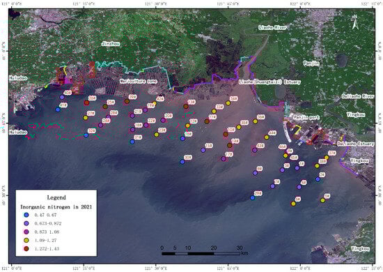
Figure 15. Inorganic nitrogen distribution data of monitoring sites in 2021.

3.7.2. Chemical Oxygen Demand

Figure 16 illustrates the distinct geographical characteristics of the Chemical Oxygen Demand (COD) indicators at the monitoring stations. The COD levels are notably high in the area where the Liao River discharges into the sea, whereas they are lower in the regions where the Daliao River and Xiaoling River enter the sea on either side. Upon analysis, it is evident that the Liao River flows through areas such as Panjin City, Dawa County, and Panshan County before reaching the sea. These regions are characterized by significant industrial activity and a concentration of heavily polluting industries. For instance, Panjin City is a major petrochemical hub in China, with numerous large-scale oil refining and chemical enterprises located nearby. Inadequate treatment of wastewater and waste by these industries may result in elevated COD levels in the water quality of the Liaohe estuary. Similar conclusions have been drawn by scholars Yang Yongli and Wu Guanghong in their studies of this area [9,62]. In contrast, the Daliao River flows through regions with fewer industrial zones, thereby minimizing the impact of industrial wastewater and waste discharges and resulting in lower COD levels in the estuary’s water quality.

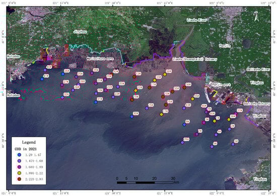
Figure 16. Distribution map of chemical oxygen demand indicators at monitoring stations in 2021.

3.8. Distance Effect Model

3.8.1. Homogeneous Shoreline Distance Effect

We initially constructed a homogeneous shoreline devoid of anthropogenic impacts and characterized by a single type of utilization, where water quality near the shoreline is influenced solely by terrestrial erosion, natural climate change, and ecosystem health. The shortest distance from each monitoring station to the shoreline was calculated using the Proximity—Near tool in ARCGIS software (ArcMap 10.7). A correlation analysis of inorganic nitrogen content with this shortest distance was conducted using SPSS 13.0 (see Table 17), yielding a Pearson correlation coefficient of −0.504, which is statistically significant at the 0.01 level. Based on this analysis, we performed a model fit for distance decay and determined that an exponential decay model more accurately represents the variation of inorganic nitrogen with distance (Figure 17). Regression analysis using SPSS 13.0 was employed for curve estimation, and the constant term and coefficients were calculated using a model with an exponential distribution (see equations below).

Table 17. Correlation analysis between inorganic nitrogen content and shoreline distance.

	Inorganic Nitrogen	Distance from Shoreline
Inorganic  Nitrogen Pearson Correlation	1	−0.504 (**)
Significance (2-tailed)		0
N	46	46
Distance  from  Shoreline Pearson Correlation	−0.504 (**)	1
Significance (2-tailed)	0
N	46	46

** Correlation is significant at the 0.01 level (2-tailed).

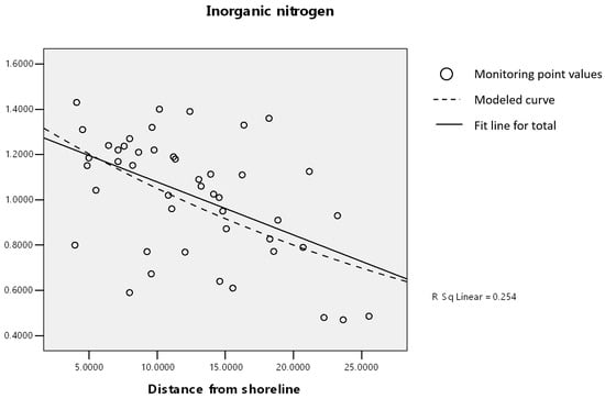
Figure 17. The inorganic nitrogen content was fitted to the shoreline distance curve.

The confidence interval of all parameters does not contain 0, which supports the conclusion of statistical significance ($p<0.001$), see Table 18.

$$Q\left(d\right)=1.3773\times e^{-0.0271d}$$

(7)

Table 18. The results of linear regression analysis of inorganic nitrogen and distance.

Parameter	Non-Normalized Coefficients	Standard Error	Standardization Coefficient	t Ratio	p-Value	95% Confidence Interval	Non-Normalized Coefficients
Constant term	1.312	0.083	-	15.784	<0.001	[1.145, 1.480]	1.312
Distance	−0.023	0.006	−0.504	−3.872	<0.001	[−0.036, −0.011]	−0.023

After curve simulation, 18 out of the 46 sites were found to have been accurately simulated, with results within 10% of the actual values (see Table 19).

Table 19. Simulation of the distance effect of inorganic nitrogen near the coast of Liaodong Bay.

Station Number	Inorganic Chemistry Nitrogen	Distance to Coastline (km)	Value of Simulation	Residuals
4	0.872	15.065	0.915	−0.043
7	0.772	18.547	0.832	−0.06
8	0.827	18.266	0.839	−0.012
9	1.169	7.119	1.135	0.034
13	1.31	4.513	1.218	0.092
15	0.79	20.705	0.785	0.005
18	0.91	18.853	0.825	0.085
19	0.96	11.062	1.020	−0.06
20	1.02	10.810	1.027	−0.007
21	1.01	14.544	0.928	0.082
22	0.95	14.809	0.921	0.029
24	1.06	13.217	0.962	0.098
36	1.24	6.424	1.157	0.083
37	1.151	4.850	1.207	−0.056
42	1.22	7.124	1.135	0.085
43	1.025	14.133	0.938	0.087
44	1.152	8.189	1.103	0.049
45	1.185	4.974	1.203	−0.01

In order to test the spatial autocorrelation of the residuals of the distance effect model, ArcGIS software was used to analyze the global Moran index. The results show that the residual Moran index is 0.009753, the z-score is 0.488148, the p-value is 0.625445, the Expected Index is −0.058824, and the Variance is 0.019736, which is not significant at the 0.05 level. This proves that the model residuals are randomly distributed in space and there is no significant spatial autocorrelation. Therefore, the model constructed in this study well explains the spatial structure of the data, and its statistical inference results are reliable.

However, the simulation results for the remaining stations were generally unremarkable. Upon comparison, a distinct shoreline effect was observed, where the deviation of simulated values for sites around a particular shoreline was more consistent. Consequently, we developed separate distance effect models for the estuary and the port shoreline. The simulation results for the port shoreline model were poor, as shown in the Table 20, indicating that the distance effect of the port on water quality in the nearshore area of Liaodong Bay is not significant. In contrast, the distance effect of the estuary on offshore water quality is more pronounced. This suggests that the construction and operation of Panjin Port have minimized its impact on the water environment, aligning with the “Eco-Port” objectives that Panjin Port aims to achieve, as outlined in the “Panjin Port Master Plan (Revised 2016) Environmental Impact Report.”

Table 20. Comparison of the simulated and real values of the port distance effect of inorganic nitrogen.

Station Number	Inorganic Nitrogen	Distance to Coastline (km)	Value of Simulation	The Gap with the Real Value
1	0.771	9.245	1.072	39%
2	0.673	9.555	1.063	58%
3	0.769	12.038	0.993	29%
5	1.113	13.922	0.944	−15%
6	1.125	21.163	0.775	−31%
29	0.486	25.547	0.688	42%
38	1.237	7.563	1.122	−9%
46	1.042	5.492	1.187	14%

3.8.2. Estuarine Distance Effect

In the study of the estuary distance model, the correlation index (see Table 21), the $R^2$ value is 0.41, the constant term is 1.702, and the distance coefficient is −0.035. The simulation effect of the curve is illustrated in Figure 18. Overall, the simulation effectively captures the influence of distance from the estuary on the distribution of inorganic nitrogen.

Table 21. Model summary and parameter estimation.

Equation	Model Summary					Parameter Estimates
	RSquare	F	df1	df2	Sig.	Constant	b1
Exponential	0.401	7.371	1	11	0.020	1.702	−0.035

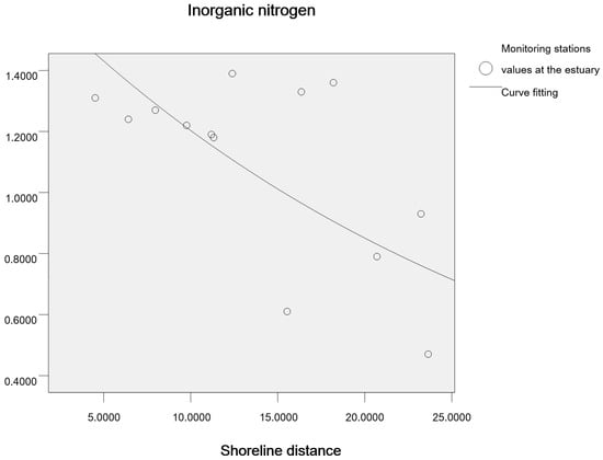
Figure 18. Simulation of estuarine distance effect of inorganic nitrogen.

Since the confidence interval does not contain 0, and the p-value (significance) is less than 0.05, these results further support the conclusion that there is a significant negative correlation between shoreline distance and inorganic nitrogen content, see Table 22.

Table 22. Results of linear regression analysis of inorganic nitrogen content.

Model	Non-Normalized Coefficients		Standardized Coefficient	t Ratio	Prominence	95% Confidence Interval of B
	B	Standard Error	Beta			Lower Limit	High Limit
Constant	1.527	0.170	–	8.973	0.000	1.153	1.902
Shoreline distance	−0.031	0.011	−0.637	−2.737	0.019	−0.055	−0.006

The estuarine distance effect was modeled, see Equation (8).

$$H\left(d_2\right)=1.701897\times e^{-0.034675d_2}$$

(8)

4. Discussion

4.1. Data Selection Problem

It is found that the stability of autumn data in 2021 is stronger than that of spring data in 2022. Therefore, autumn data in 2021 are often used as important data sources for analysis, and spring data in 2022 are used as auxiliary data sources. However, whether this selection standard is reasonable requires more period data to support. When some scholars studied the influence of wet and dry seasons on the phytoplankton community structure, they found that the phytoplankton species were abundant in the wet season, the number of cells was high, and a high-value area was formed in the coastal waters. In the dry season, the number of species was small, the number of cells was low, and a high-value area was formed in the offshore waters [63].

In addition, in the study, unreasonable data are not eliminated, which will also affect the analysis of the results and the simulation of the model. It needs to be gradually supplemented and improved in future research.

4.2. Model Simulation Problem

The effect of model simulation should be based on the test of multi-sequence data. At present, there are few data sequences, and the model may over-adapt to limited data, resulting in poor performance on new and unseen data. The parameter estimation in the model may also have large errors; with less data, it may be difficult to verify the authenticity of these hypotheses. Based on the above, we need to treat the simulation results with caution and recognize their potential uncertainties and limitations. In the future work, we need to collect more monitoring station data to improve the generalization ability and accuracy of the model.

4.3. Shoreline and Sea Area Use Issues

The coastline and sea area use types of Liaodong Bay are not very complex. Although they have a certain degree of impact on the water quality of the coastal waters, they have not yet become the primary factor. At present, the water quality of rivers entering the sea is still the primary factor affecting the water quality of coastal waters. The underlying surface type of the river flowing through the area will have a major impact on water quality. At present, the lower reaches of the Liaohe River flowing through Panjin City and surrounding districts and counties are urban and industrial distribution areas, and their water quality is deeply affected. The water quality of Daliao River and Xiaoling River is relatively good without major urban and industrial distribution areas. Therefore, the water quality monitoring data of coastal waters are also good. Therefore, in the protection of water quality in coastal waters, we should also focus on the water quality of rivers entering the sea. In the Liaodong Bay area, the water quality of the Liaohe River is the main contradiction.

4.4. Analysis of the Multiple of Land-Based Pollution

The inorganic nitrogen in the estuary of Liaohe River exceeds the standard (the average value in 2022 is 0.865 mg/L, and the national minimum standard is 0.5 mg/L), which is closely related to the industrial emissions in Panjin Oilfield. Sun et al. [11] pointed out in the study of total nitrogen and total organic carbon in the sediments of Bohai Bay that terrigenous materials in rivers are also an important source of sediments in Bohai Sea. Wu et al. [12] pointed out in the study of Bohai Bay that the concentration of polycyclic aromatic hydrocarbons in Bohai Sea showed a decreasing trend to the sea. Concentrations in river sediments were higher (445–2190 ng/g, mean 964 ng/g), while concentrations in offshore sediments were lower (171–290 ng/g, mean 226 ng/g). PAHs pollution is characterized by terrestrial input through river-estuary-bay pathways.

4.5. Regional Heterogeneity of Biological Community Response

The phytoplankton diversity index (mean 3.52) was 20% lower in the aquaculture area on the west side of the Liaohe Estuary (monitoring station 42#) than in the large Liaohe Estuary on the east side (monitoring station 6#). This is consistent with the increase of phytoplankton diversity observed by Li [38] in the Yangtze Estuary. The diversity of phytoplankton is rich in nitrogen and phosphorus nutrients brought by terrestrial input in the estuary area, and the mixing of salt and fresh water in the estuary area promotes the growth of phytoplankton. However, this study found that the richness of zoobenthos in the adjacent area of Panjin Port (monitoring station 8#) showed a downward trend (d = 0.63). Naser’s [16] experimental analysis of the impact of reclamation and reconstruction projects on macrobenthic communities in the Arabian Gulf showed that there was a significant difference in the number of surviving organisms between the control group and the experimental group. The survival rate of all selected species was only 41.8%, indicating that reclamation and other shoreline construction projects have a significant impact on marine benthic communities in the bay area. Janetski and Ruetz (2015) [64] found that geographical distance was negatively correlated with community similarity, indicating that dispersal and/or environmental gradients played a role in the formation of these estuarine fish communities. Cocksedge et al. (2024) [65] studied the microbial community in temperate estuaries. The results showed that the attenuation pattern of archaeal biogeographic distance within and between temperate estuaries existed at a medium spatial scale, revealing the role of spatial scale in shaping microbial communities.

5. Conclusions

This study integrated data collected during the fall of 2021 and the spring of 2022 from 46 water quality monitoring stations in Liaodong Bay to examine the impacts of shoreline development and utilization on nearshore water quality, as well as the effects of distance on water quality. The main conclusions are as follows:

1.

The water quality in the coastal waters of Liaodong Bay is generally good, but the content of inorganic nitrogen generally exceeds the level specified in the standard. This is mainly related to urban industrial emissions in the Liaohe River Basin.

2.

The concentrations of pollutants in the port area and the estuary area are generally higher than those in the peripheral sea area; this trend was verified through cluster analysis and interpolation simulations.

3.

The distribution of inorganic nitrogen was negatively correlated with the distance from the shoreline, showing a trend of distance attenuation. The constructed homogeneous shoreline distance effect model fitted well in the non-estuary area ($R^2$ = 40.1%), while a radial basis function should be introduced for correction when analyzing the estuary area.

4.

There were significant differences in the diversity, evenness, and richness indices for phytoplankton and zoobenthos among different functional areas, and these differences showed a certain gradient correlation with the intensity of human activity.

5.

The results suggest that a strategy consisting of ‘total nitrogen and phosphorus control + ecological compensation’ can be considered in the port area, while the construction of artificial reefs should be promoted in the aquaculture area. These measures may help to alleviate ecological pressure and improve system stability.

References

- Zhang, K.; Pan, S.; Liu, Z.; Li, G. Distribution pattern and source of 137Cs in the sediment cores from the Liao River Estuary. Mar. Geol. Quat. Geol. 2019, 39, 91–99. [Google Scholar] [CrossRef]
- Jin, W.; Shao, X. Analysis of Water Quality in Coastal Waters and Its Impact on the Marine Ecological Environment. J. Sci. Teach. Coll. Univ. 2000, 20, 20–23. [Google Scholar]
- Wang, L. Study on the Implementation of Marine Environmental Assessment Model in Geographic Information System. J. Comput. Appl. 2004, 132–134. [Google Scholar]
- Xin, D.; Ren, S.; Xia, J. Analysis and Synthetic Evaluation on Ecological Environment Quality in Sea Waters near Qidong Foreland in Jiangsu. Mar. Environ. Sci. 2009, 28, 28–30+42. [Google Scholar]
- Awaleh, M.; Bouraleh, H.F.; Soubaneh, Y.; Badran, M.; Bahga, H.; Samaleh, A. Impact of human activity on marine and coastal environment in the Gulf of Tadjourah. J. Mar. Science. Res. Dev. 2015, 5, 162. [Google Scholar]
- Uddin, M.G.; Nash, S.; Rahman, A.; Olbert, A.I. A comprehensive method for improvement of water quality index (WQI) models for coastal water quality assessment. Water Res. 2022, 219, 118532. [Google Scholar] [CrossRef] [PubMed]
- Wang, Y.; Zhu, D. Tidal Flats of China. Quat. Sci. 1990, 291–300. [Google Scholar]
- Kexin, Z. Distribution and Source Identification Ofthe Radionuclide 137 Cs 239+240 pu in the Sediments of the Liao River Estuary. Ph.D. Thesis, Nanjing University, Nanjing, China, 2016. [Google Scholar] [CrossRef]
- Wu, G.; Qiu, M.; Li, J.; Wei, L. Spatial-temporal variation of water quality and pollutant source analysis in rivers along Liaodong Bay. Haiyang Xuebao 2023, 45, 177–188. [Google Scholar]
- An, C. Ecological Study on Macrobenthic Animal Communities in the Intertidal Zone of the Yangtze River Estuary. Ph.D. Thesis, East China Normal University, Shanghai, China, 2011. [Google Scholar]
- Sun, C.; Wei, Q.; Ma, L.; Li, L.; Wu, G.; Pan, L. Trace metal pollution and carbon and nitrogen isotope tracing through the Yongdingxin River estuary in Bohai Bay, Northern China. Mar. Pollut. Bull. 2017, 115, 451–458. [Google Scholar] [CrossRef]
- Wu, G.; Qin, R.; Luo, W. Polycyclic aromatic hydrocarbons (PAHs) in the Bohai Sea: A review of their distribution, sources, and risks. Integr. Environ. Assess. Manag. 2022, 18, 1705–1721. [Google Scholar] [CrossRef]
- Fan, X.; Liu, L. Research Progress on Application of Bioremediation Technology in Petroleum Pollution Control. Mod. Chem. Ind. 2021, 41, 64–68. [Google Scholar] [CrossRef]
- Feng, A.; Wang, X.; Xu, Y.; Huang, L.; Wu, C.; Wang, C.; Wang, H. Assessment of Potential Risk of Diffuse Pollution in Haihe River Basin Based Using DPeRS Model. Environ. Sci. 2020, 41, 4555–4563. [Google Scholar] [CrossRef]
- Sun, Y.; Shen, Y.; Dai, L.; Zhao, W.; Wu, Y.; Zhu, L. Zooplankton Distribution and Influencing Factors in the Yellow Sea in Summer and Winter. Period. Ocean Univ. China 2020, 50, 82–93. [Google Scholar] [CrossRef]
- Naser, H.A. Effects of reclamation on macrobenthic assemblages in the coastline of the Arabian Gulf: A microcosm experimental approach. Mar. Pollut. Bull. 2011, 62, 520–524. [Google Scholar] [CrossRef]
- Wang, S.; Miao, Z.; Sheng, Q.; Zhao, F.; Wu, J. Effects of Saltmarsh Dike Project on Benthic Community in Chongming Dongtan of the Yangtze Estuary. Acta Ecol. Sin. 2020, 40, 1021–1030. [Google Scholar] [CrossRef]
- Jeppesen, E.; Nõges, P.; Davidson, T.A.; Haberman, J.; Nõges, T.; Blank, K.; Lauridsen, T.L.; Søndergaard, M.; Sayer, C.; Laugaste, R.; et al. Zooplankton as indicators in lakes: A scientific-based plea for including zooplankton in the ecological quality assessment of lakes according to the European Water Framework Directive (WFD). Hydrobiologia 2011, 676, 279–297. [Google Scholar] [CrossRef]
- Sutherland, R.J.; Walsh, R.G. Effect of distance on the preservation value of water quality. Land Econ. 1985, 61, 281–291. [Google Scholar] [CrossRef]
- Hanink, D.M. The economic geography in environmental issues: A spatial-analytic approach. Prog. Hum. Geogr. 1995, 19, 372–387. [Google Scholar] [CrossRef]
- Pan, B. Research on Carbon Storage of Major Aquatic Plant Communities. Master’s Thesis, Nanjing Forestry University, Nanjing, China, 2013. [Google Scholar]
- Li, J.; Zhang, M. A Study on Willingness to Pay for the Management of Enteromorpha Prolifera in Qingdao Based on Spatial Distance Effect. Ocean Dev. Manag. 2024, 41, 117–125. [Google Scholar] [CrossRef]
- Tao, X.; Qi, N.; Dan, Q.; Liuyang, Y.; Minjuan, Z. Distance Effect on the Willingness of Rural Residents to Participate in Watershed Ecological Restoration: Evidence from the Shiyang River Basin. Resour. Sci. 2020, 42, 1395–1404. [Google Scholar]
- GB 17378-2007; The specification for marine monitoring. State Administration for Market Regulation, National Standardization Administration: Beijing, China, 2007.
- GB 12763-2007; Specifications for oceanographic survey. State Administration for Market Regulation, National Standardization Administration: Beijing, China, 2007.
- GB 17378.4-2007; The specification for marine monitoring—Part 4: Seawater analysis. State Administration for Market Regulation, National Standardization Administration: Beijing, China, 2007.
- GB/T 12763.6-2007; Specifications for oceanographic survey—Part 6: Marine biological survey. National Standardization Administration: Beijing, China, 2007.
- GB 17378.7-2007; The specification for marine monitoring—Part 7: Ecological survey for offshore pollution and biological monitoring. State Administration for Market Regulation, National Standardization Administration: Beijing, China, 2007.
- HJ 442-2020; Technical specification for offshore environmental monitoring. Ministry of Ecology and Environment of the People’s Republic of China: Beijing, China, 2020.
- HJ 442.10-2020; Technical specification for offshore environmental monitoring Part 10 evaluation and report. Ministry of Ecology and Environment of the People’s Republic of China: Beijing, China, 2020.
- GB 3097-1997; Sea water quality standard. Ministry of Ecology and Environment of the People’s Republic of China. State Administration for Market Regulation, National Standardization Administration: Beijing, China, 1997.
- GB 18668-2002; Marine sediment quality. State Administration for Market Regulation, National Standardization Administration: Beijing, China, 2002.
- GB 18421-2001; Marine biological quality. State Administration for Market Regulation, National Standardization Administration: Beijing, China, 2001.
- Shannon, C.E. A mathematical theory of communication. Bell Syst. Tech. J. 1948, 27, 379–423. [Google Scholar] [CrossRef]
- Margalef, R. Information theory in ecology. Int. J. Gen. Syst. 1958, 3, 36–71. [Google Scholar]
- Pielou, E.C. Species-diversity and pattern-diversity in the study of ecological succession. J. Theor. Biol. 1966, 10, 370–383. [Google Scholar] [CrossRef]
- Xu, Z.; Wang, Y.; Chen, Y.; Shen, H. An Ecological Study on Zooplankton in Maximum Turbid Zone of Estuarine Area of Changjiang (Yangtze) River. J. Fish. Sci. China 1995, 2, 10. [Google Scholar]
- Li, L.; Wang, Y.; Wang, B.; Lu, S.; Lei, K.; He, B.; Cheng, Q. Spatiotemporal Distribution of Plankton Community Structure in the Yangtze River Estuary in the Summer of 2009–2021 and Its Influencing Factors. Res. Environ. Sci. 2024, 37, 233–245. [Google Scholar] [CrossRef]
- Gregory, E. Fasshauer, Meshfree Approximation Methods with MATLAB; World Scientific Publishing Co.: Singapore, 2007. [Google Scholar]
- Wang, Q. Minister’s Research Focuses on Excessive Total Nitrogen in Inflow Rivers: What Are the Current Governance “Good Solutions”? China Environment News 2023. [Google Scholar]
- Lü, X.; Xu, H.; Zhao, S.; Kong, F.; Yan, T.; Jiang, P. The green tide in Yingkou, China in summer 2021 was caused by a subtropical alga—Ulva meridionalis (Ulvophyceae, Chlorophyta). J. Oceanol. Limnol. 2022, 40, 2354–2363. [Google Scholar] [CrossRef]
- Zhou, Z.; Pan, S.; Yang, P. The Application of SPSS Fuzzy Clustering Analysis on Water Quality Monitoring Sections. Instrum. Anal. Monit. 2007, 32–33+35. [Google Scholar]
- Qian, S.; Chen, G. Phytoplankton Biology. Period. Ocean. Univ. China 1986, 26–55+85–86. [Google Scholar] [CrossRef]
- Wang, Y.; Lin, M.; Lin, G.; Wang, C.; Xiang, P. Yearly Changes of Phytoplankton in the Ecological Monitoring Zone of Daya Bay. Mar. Sci. 2012, 36, 86–94. [Google Scholar]
- Wang, W.; He, J.; Fu, P.; Jiang, H.; Wang, N.; Liu, A.; Song, X.; Cheng, L. Interannual variation of the phytoplankton community and its relationship with environmental factors in Miaodao Archipelago waters. J. Fish. Sci. China 2022, 29, 1002–1012. [Google Scholar]
- Huang, D.; Huang, Z.; Huang, W.; Wu, W. Plankton in Hengqin Island Sea in the Pearl River Estuary in Spring. Ecol. Sci. 2009, 28, 342–347. [Google Scholar]
- Qin, C.; Sun, K.; Chen, Q. Assessment and Analysis of Marine Ecological Environment Quality in the Coastal Waters of Jiangmen City in Spring. In Proceedings of the 2017 Annual Conference on Science and Technology, Chinese Society for Environmental Sciences (Volume 3), Suzhou, China, 23–25 June 2017; South China Institute of Environmental Sciences, Ministry of Environmental Protection: Guangdong, China, 2017; pp. 586–593. [Google Scholar]
- Zhou, R. Temporal Changes of Marine Phytoplankton Communities and Influential Factors of Bohai Bay, China. J. Waterw. Harb. 2012, 33, 72–76. [Google Scholar]
- Navarro, G.; Ruiz, J. Spatial and temporal variability of phytoplankton in the Gulf of Cádiz through remote sensing images. Deep Sea Res. Part II Top. Stud. Oceanogr. 2006, 53, 1241–1260. [Google Scholar] [CrossRef]
- Gao, Q.; Xu, Z.; Zhuang, P. The relation between distribution of zooplankton and salinity in the Changjiang Estuary. Chin. J. Oceanol. Limnol. 2008, 26, 178–185. [Google Scholar] [CrossRef]
- Gao, L.; Li, D.; Ishizaka, J.; Zhang, Y.; Zong, H.; Guo, L. Nutrient dynamics across the river-sea interface in the Changjiang (Yangtze River) estuary—East China Sea region. Limnol. Oceanogr. 2015, 60, 2207–2221. [Google Scholar] [CrossRef]
- Zheng, Z. The Structure of Zooplankton Communities and Its Seasonal Variation in the Yellow Sea and in the Western East China Sea. Oceanol. Et Limnol. Sin. 1965, 199–204. [Google Scholar]
- Sun, S.; Huo, Y.; Yang, B. Zooplankton functional groups on the continental shelf of the yellow sea. Deep Sea Res. Part II Top. Stud. Oceanogr. 2010, 57, 1006–1016. [Google Scholar] [CrossRef]
- Wang, L.; Li, C.; Yu, F. Zooplankton Community Structure in the South Yellow Sea in Winter and Indication of the Yellow Sea Warm Current. Oceanol. Limnol. Sin. 2013, 44, 853–859. [Google Scholar]
- Ding, F.; Li, S.; Dong, J.; Cheng, J. Preliminary Study on the Zooplankton Community Structure and Its Influential Factors in the Offshore Waters of the East China Sea in Spring. Mar. Fish. 2005, 26–32. [Google Scholar]
- Zhu, Y.; Liu, L.; Zheng, B.; Wang, Y. Relationship Between Spatial Distribution of Zooplankton and Environmental Factors in the Changjiang Estuary and Its Adjacent Waters in Spring. Mar. Sci. 2011, 35, 59–65. [Google Scholar]
- Pang, B.; Li, T.; Lan, W.; Li, M.; Luo, X.; Chen, Y. Distribution Patterns and Environmental Factors of Zooplankton in the Qinzhou Bay in Spring and Autumn. Acta Ecol. Sin. 2018, 38, 6204–6216. [Google Scholar] [CrossRef]
- Liu, C.; Wang, R.; Gao, H.; Wang, P.; Yin, D. Distribution and Factors Influencing Macro- and Meso-Plankton in the Yangtze River Estuary–East China Sea Continental Shelf in Summer. J. Tongji Univ. (Natural Sci.) 2021, 49, 1363–1373+1350. [Google Scholar]
- Xu, H.; Zhao, Y. Scientific Expedition Report of the Chongming Dongtan Bird Nature Reserve in Shanghai; China Forestry Publishing House: Beijing, China, 2005. [Google Scholar]
- Yang, J.; Zheng, M.; Wang, Q.; Xue, J.; Wu, H. Influence of Different Tideland Reclamation Ways on Macrobenthic Communities. Resour. Environ. Yangtze Basin 2016, 25, 1358–1367. [Google Scholar]
- Liu, J.; Xia, W.; Zhao, L.; Ma, Q. Petroleum Contaminants in Seawater and Their Bioremediation. Trans. Oceanol. Limnol. 2006, 48–53. [Google Scholar] [CrossRef]
- Yang, Y. Comprehensive Evaluation of River Water Quality in Liaohe River Basin. Water Resour. Dev. Manag. 2021, 28–32+56. [Google Scholar] [CrossRef]
- Li, Z.; Song, S.; Li, C.; Yu, Z. Preliminary discussion on the phytoplankton assemblages and its response to the environmental changes in the Changjiang (Yangtze) River Estuary and its adjacent waters during the dry season and the wet season. Haiyang Xuebao 2017, 39, 124–144. [Google Scholar] [CrossRef]
- Janetski, D.J.; Ruetz, C.R., III. Spatiotemporal patterns of fish community composition in Great Lakes drowned river mouths. Ecol. Freshw. Fish 2015, 24, 493–504. [Google Scholar] [CrossRef]
- Cocksedge, E.; Stat, M.; Suzzi, A.L.; Gaston, T.F.; Huggett, M.J. Spatial and environmental drivers of temperate estuarine archaeal communities. Mar. Environ. Res. 2024, 201, 106703. [Google Scholar] [CrossRef]
Disclaimer/Publisher’s Note: The statements, opinions and data contained in all publications are solely those of the individual author(s) and contributor(s) and not of MDPI and/or the editor(s). MDPI and/or the editor(s) disclaim responsibility for any injury to people or property resulting from any ideas, methods, instructions or products referred to in the content. |
© 2026 by the authors. Licensee MDPI, Basel, Switzerland. This article is an open access article distributed under the terms and conditions of the Creative Commons Attribution (CC BY) license.