Abstract
Accurate runoff simulation is essential for water resources planning and development projects. At present, the commonly employed runoff simulation approaches are categorized into two types: process- and data-driven models. Process-driven models pertain to the enhancement of the structural framework in conceptual rainfall–runoff models using hydrological principles to estimate runoff but have low accuracy at the monthly scale. Unlike the process-driven models, data-driven models (DDMs) can simulate the relationship between input factors and output runoff data without regard to complex and unknown runoff production and acquire satisfactory simulation results. Here, we comparatively investigate the applicability of DDMs, including traditional shallow DDMs, deep learning-based (DL) models for monthly runoff simulation, and select the Autoregressive (AR) model as the baseline model for comparison. Moreover, four evaluation indicators, including mean absolute percentage error (MAPE), root mean squared error (RMSE), Nash–Sutcliffe efficiency (NSE), and coefficient of determination (R2), are employed to evaluate the runoff simulation effects of the above methods. We systematically compare the AR model, and shallow and deep learning-based DDMs for runoff simulation at four hydrological stations in the Yalong River basin (YRB), respectively. The finding results reveal that the DDMs demand limited data and can offer satisfactory prediction effects. Also, the DL models outperform other shallow DDMs and the AR model in terms of the above evaluation criteria.
1. Introduction
Accurate runoff simulation is essential for water resources planning and development projects and has increasingly attracted attention as a crucial and complex topic in hydrology [1,2,3]. However, runoff time series usually introduce redundant and noisy information because of climate change and human activities [4]. As a result, the runoff simulation exhibits randomness, uncertainty, and complex nonlinear characteristics, which seriously affect the runoff simulation effect [5]. Accordingly, it is a great challenge to design optimal simulation models for improving the accuracy of runoff simulation [6].
At present, aiming to enhance the accuracy of runoff simulation, some runoff simulation models have been developed, mainly including two categories: process- and data-driven models [7,8]. Process-driven models (PDMs) usually adopt numerical forecasting products as the input of the hydrological model, and the accuracy of numerical forecasting products significantly influences the performance of the forecasting system [9]. For example, the SAC-SMA model has been extensively applied in rainfall–runoff modeling, such as streamflow simulation and soil studies [10,11,12]. Behrangi et al. [12] proposed the SAC-SMA model for streamflow simulation and obtained good results. Chu et al. [13] applied the SP-UCI method for calibrations of the SAC-SMA model and acquired the optimal calibration results. Another typical process-based hydrologic model is the Xin’anjiang (XAJ) hydrological model, which has been widely used in humid and semi-humid regions [14,15,16]. For example, Fang et al. [17] improved the original XAJ hydrological model, called the XAJ-EB model, and extended the applicability. Xu et al. [18] developed the three global optimization algorithms to search parameters of XAJ hydrological model and obtained better results in likely applications of XAJ hydrological model. The PDMs have been widely applied to hydrology, but these models have low accuracy at the monthly scale, especially when the prediction period exceeds one month; the simulation accuracy sharply decreases, and it cannot achieve a good prediction effect. In addition, the above methods rely on detailed surface conditions and more relevant data as support, which hinders the development of PDMs.
Compared with the PDMs, the data-driven models (DDMs) exhibit the advantages of high precision and robustness without regard to the physical mechanism of hydrological processes and thus has been extensively applied in runoff simulation [19,20]. Traditional DDMs are applied to runoff simulation, such as Artificial Neural Network (ANN), Support Vector Machine (SVM), Extreme Learning Machine (ELM), and multiple combination models. For instance, Yazdani et al. [21] selected the ANN for runoff estimation and achieved good effects. Samantaray et al. [22] adopted the SVM coupled with the salp swarm algorithm for monthly runoff prediction and promoted the prediction accurateness. Yaseen et al. [23] developed the ELM model for streamflow prediction, which demonstrated superior performance compared with the GRNN and SVR models. He et al. [24] proposed the novelty hybrid DDM for the runoff prediction and reached higher accuracy. Li et al. [25] employed five ML models to forecast monthly runoff, and the LSTM_Copula model performed best.
Traditional DDMs demonstrate good performance in monthly runoff simulation. Nevertheless, these models have shallow model structures; the parameters of models need to be initialized, optimized constantly, and cannot acquire accurate runoff prediction results. Currently, more and more deep learning-based (DL) models have been applied in the field of hydrological simulation, such as Long Short-term Memory (LSTM), convolutional neural network (CNN), and Deep Belief Networks (DBNs) [26]. In comparison with shallow networks, the deep learning-based models can calculate via layer-by-layer transmission to learn too much intrinsic characteristics. The deep learning-based models can compensate for the shortcomings of shallow DDMs and enhance the runoff simulation accuracy, speed, and robustness. For example, Van et al. [27] developed a novel 1D convolutional neural network (CNN), with a ReLU activation function for rainfall–runoff modeling, and the experimental results revealed that both CNN and LSTM had better simulation effects than the traditional models. Yue et al. [5] developed a novel hybrid data-driven model called PSO-FPA-DBNs for monthly runoff forecasting, achieving good forecasting results. Wang et al. [28] designed the WOA-VMD-LSTM model and achieved good runoff prediction results. The findings showed that the proposed model increased the accuracy of point predictions and provided high-quality prediction intervals.
The Yalong River basin (YRB) is characterized by a plateau climate with a wet and dry season, has abundant runoff and rich hydropower resources, and plays a crucial role in China’s western development and optimal allocation of water resources. Therefore, it is necessary and crucial to conduct research on the monthly runoff simulation in the YRB. In addition, the relevant literature on monthly runoff simulation in the YRB mainly focuses on the single machine learning method, and seldom conducts comparative study of the shallow and deep learning-based DDMs at four stations in the YRB. Based on these, the aim of this study is to comparatively investigate the applicability of shallow and deep learning-based DDMs (ANN, SVM, ELM, LSTM, CNN, DBN), and the Autoregressive (AR) model for monthly runoff simulation. The main contributions of this research can be outlined as follows:
(1) Monthly runoff was simulated at four hydrological stations in the YRB, respectively.
(2) The shallow and deep learning-based DDMs (ANN, SVM, ELM, LSTM, CNN, DBN) and the AR model were used.
(3) Less error and better simulation effect was achieved by the deep learning models.
The remainder of this paper is structured as follows. Section 1 provides the introduction and literature review. Section 2 presents the methodologies used in this study, including six commonly used shallow and deep learning-based DDMs. Section 3 provides comprehensive details regarding study area and data. Section 4 summarizes data pre-processing, factors selection, and monthly runoff training and simulation results at four hydrological stations in the Yalong River basin. Section 5 presents the analysis and discussion of the results, while Section 6 provides the summary of our conclusions. Figure 1 illustrates the overall research framework of different models used for monthly runoff simulation.
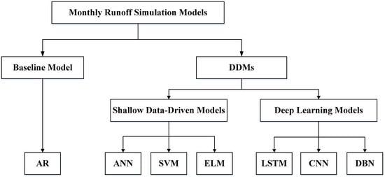
Figure 1.
The overall research framework of different models used for monthly runoff simulation.
2. Methodology
2.1. Shallow Data-Driven Models
2.1.1. ANN
The ANN model is a nonlinear model that mimics the biological processes of human cognition and neural systems by a mathematical model. Similarly to the human brain, ANN is a simple network and interconnected by billions of processing units called neurons, which may automatically adjust to the connection weights and mimic the nonlinear learning process. Detailed descriptions of the ANN are not provided in this paper. Instead, we suggest that the interested reader refer to the relevant literature [29,30]. The structure of the ordinary ANN model includes an input layer, a hidden layer, and an output layer (Figure 2).
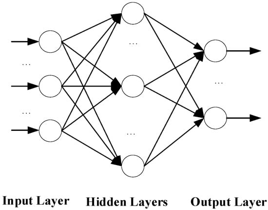
Figure 2.
The structure of the ordinary ANN model.
2.1.2. SVM
The SVM model is based on the Vapnik Chervonenkis (VC) dimension theory which is applied to a linear model in order to transform a specific problem into a quadratic optimization problem, thereby obtaining a global optimal solution, and effectively solving problems such as high dimensionality, nonlinearity, and local minima [20]. The basic structure of SVM model is shown in Figure 3.
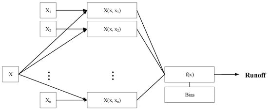
Figure 3.
The basic structure of SVM model.
2.1.3. ELM
The weights and biases of the input layer in ELM model are given randomly, and the weights of the output layer are solved by generalized inverse matrix, which can not only reduce the adjustment times of network parameters but also effectively save the training time [31]. As a result, ELM benefits from simple model structure, good learning capability, and is prominently efficient to reach a global optimum solution. In recent years, ELM model has been widely applied to hydrological forecasting [3,23,32]. Figure 4 shows the ordinary ELM’s structure.
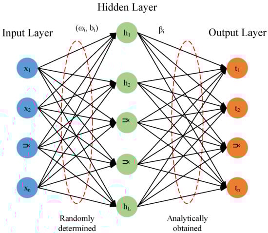
Figure 4.
The structure of the ordinary ELM model: the red boxes represent the weights of the input layer and hidden layer, as well as the weights of the hidden layer and output layer.
2.2. Deep Learning Models
2.2.1. LSTM
The LSTM model is a specialized form of recurrent neural network (RNN) developed to address the problems of gradient vanishment commonly encountered in traditional RNN [33,34]. The LSTM model excels in time series forecasting by connecting historical data with present observations, specializing in runoff simulation. A detailed explanation of LSTM model is not provided in this paper. Instead, for detailed descriptions of LSTM, please see the reference [35]. Figure 5 shows the ordinary LSTM’s structure.
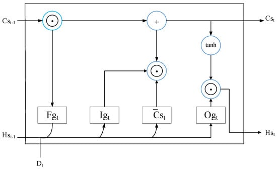
Figure 5.
The structure of the ordinary LSTM model: according to the input gate Igt and output gate Ogt, the memory cell state Cst and hidden state Hst would be updated selectively. In addition, the irrelevant information in long-term memory would be forgotten by forget gate Fgt.
2.2.2. CNN
CNN is an improved neural network that has strong adaptability and performs well in mining inherent data features [36,37]. Sparse connections and weight sharing are the most notable features of CNN. For detailed descriptions of the principles of the CNN, please see the reference [38]. Figure 6 shows the structure of the ordinary CNN model.
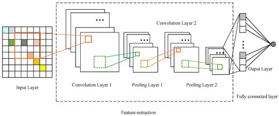
Figure 6.
The structure of the ordinary CNN model: the ordinary CNN model generally comprised five types of layers: input, convolution, pooling, fully connected, and output layers.
2.2.3. DBN
The ordinary DBN model consists of restricted Boltzmann machines (RBM), back propagation (BP) neural networks, and softmax classifiers. The training process is divided into unsupervised and supervised stages. The greedy training algorithm has advantages of fast parameter determination and accurate feature extraction and thereby has been introduced to train the DBN model. The whole learning algorithm includes two stages: (i) RBM pre-training, which intends to learn the data feature and initialize parameters of the DBN; (ii) fine-tuning, which usually adopts the BP algorithm to fine-tune the parameters of the DBN [5]. Figure 7 illustrates the architecture of the conventional DBN model.
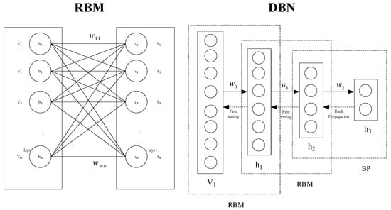
Figure 7.
The architecture of the conventional DBN model.
2.3. Evaluation Criteria
In order to evaluate the runoff simulation effects of the DDMs, four evaluation indicators were utilized [3,9]: mean absolute percentage error (MAPE), root mean squared error (RMSE), Nash–Sutcliffe Efficiency (NSE), and coefficient of determination (R2). In general, a smaller value for MAPE and RMSE, and closer values to 1 for NSE indicate better performance of the model. The closer values to 1 for R2, which denotes the higher degree of fitting between the predicted values and actual values.
3. Study Region and Data
The YRB is a natural treasure trove of green energy with abundant water and huge drops; 22 hydropower stations have been planned, with a total installed capacity of approximately 30 million kilowatts and an annual power generation of approximately 150 billion kilowatt hours [2] (Figure 8).
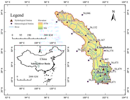
Figure 8.
The overview of the YRB.
This study covers the time range from January 1960 to December 2011. The dataset includes runoff, rainfall, and 95 teleconnection climate factors. The period 1960.01–2001.12 was used for training, and 2002.01–2011.12 for validation. Figure 9 showcases the historical runoff data from the Lianghekou (LHK), Jinping (JP), Guandi (GD), and Ertan (ET) hydrological stations. The statistical measures (e.g., min, max, ave, STDEV, etc.) of the runoff data used in this study are summarized in Table 1.
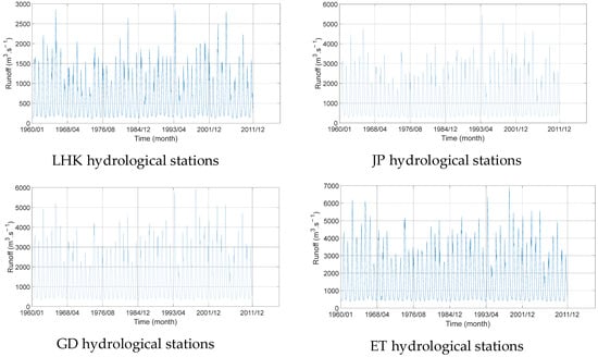
Figure 9.
Original monthly runoff series from four hydrological stations.

Table 1.
The statistical measures of the runoff data from four hydrological stations.
4. Results and Discussion
In this section, the traditional shallow DDMs, deep learning-based (DL) models, and the Autoregressive (AR) model for monthly runoff simulation were applied, including Data Pre-processing, Factors Selection Results, Model Development, and Monthly Runoff Training and Validation Results.
4.1. Data Pre-Processing
According to previous relevant studies [39,40], the data pre-processing method was chosen for standardization and normalization in this study.
4.2. Factors Selection Results
In this study, the alternative candidate predictive factors consisted of the measured values of 97 variables including 95 teleconnection climate factors (accessible at http://cmdp.ncc-cma.net/cn/monitoring.htm (accessed on 11 May 2025); http://data.cma.cn (accessed on 11 May 2025)), runoff, and area rainfall from the previous 12 months in the YRB.
Consequently, we selected the candidate factors including monthly average runoff (mar (m-1), mar (m-2), …, mar (m-12)), area rainfall (rf (m-1), rf (m-2), …, rf (m-12)), and 95 teleconnection climate factors (cli1 (m-1), cli1 (m-2), …, cli1 (m-12), cli2 (m-1), cli2 (m-2), …, cli2 (m-12), …, cli95 (m-1), cli95 (m-2), …, cli95 (m-12)). The total number of predictive factors is 1164 (97 × 12). According to the references [41,42], Pearson’s correlation coefficient and stepwise regression analysis methods were applied to select input factors. As a result, the factors selection results at four stations were set as shown in Table 2 and Table 3, respectively.
Table 2.
Factors selection results at four hydrological stations.
Table 3.
The interpretations of selected key factors.
4.3. Parameters Settings
In this study, the rainfall, evaporation, and runoff data covering the period from January 1960 to December 2001 at LHK, JP, GD, and ET hydrological stations were selected for model training.
Based on the training dataset, all the simulations of DDMs were implemented in the MATLAB R2016a (9.0.0.341360) software modeling tools. Generally, the selection of the learning rate is critical for DDMs. If the learning rate is set too small, the neural network may exhibit slow learning efficiency. Conversely, an excessively large learning rate can cause the network to fail to converge. Consequently, we fixed other hyperparameters of models and adopted the trial-and-error approach to determine the optimal learning rates of the ANN, LSTM, CNN, and DBN in this study. The initial learning rate range was set as 0.001–0.01, with a step size of 0.001, while the best models were evaluated by minimum RMSE in the training stage. The calculation results based on the training set are as shown in Figure 10.
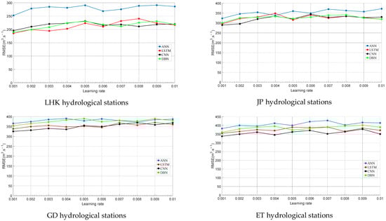
Figure 10.
Selection process of learning rates of different models at four hydrological stations.
As shown in Figure 10, we can see that when the learning rate was 0.001, the RMSEs of the four machine learning models at the four hydrological stations were the smallest. Therefore, we selected the learning rate as 0.001. The parameters of DDMs were set as follows.
(1) ANN
In ANN, the number of nodes was 12 in the hidden layer and the “tansig” and “logsig” were selected as training and learning functions, respectively. The maximum number of training iterations was 1000, the learning rate was 0.001, and the expected error was 0.001.
(2) SVM
In SVM, the kernel function was “sigmoid”, and parameter optimization method was the grid-search algorithm. For detailed descriptions of the SVM model, please see the reference [43].
(3) ELM
For ELM, selecting the “sigmoid” as the excitation function. The initial number of hidden layer nodes was 5, and the number of hidden layer nodes in ELM gradually increased, with a step size of 2. The model that achieved the smallest RMSE value in the training period was considered the optimal model. For detailed descriptions, refer to the relevant literature [23,32].
(4) LSTM
According to Li et al. [25], the parameters of LSTM were configured as follows: the num_layers and batch_size were set to 2 and 120, respectively, and the hidden_size was selected from 10 to 120. The maximum training times was 1000 and the learning rate was set as 0.001.
(5) CNN
According to the existing mature research results [38], each convolution layer had only one channel and the hyperparameter settings of the CNN in this study were as follows: the batch_size was set to 120, the maximum training times was 1000, the learning rate was set as 0.001, and the kernel size was set as 2.
(6) DBN
The DBN model included three hidden layers, and the initial number of hidden layer nodes was 12. The initial learning rates were 0.01 and 0.001 at the pre-training and fine-tuning stages, respectively. The training iterations were 1000.
4.4. Monthly Runoff Training Results
The monthly runoff training results of the shallow DDMs, deep learning-based (DL) models, and AR model are shown in Figure 11, Figure 12, Figure 13 and Figure 14. Performance comparison of the seven models based on the training results at different stations are shown in Table 4.
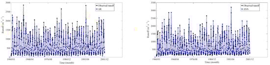
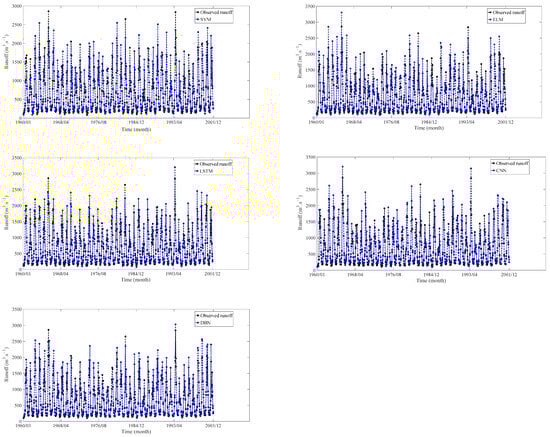
Figure 11.
Training results at LHK hydrological station.
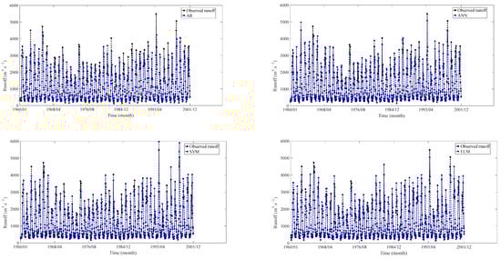
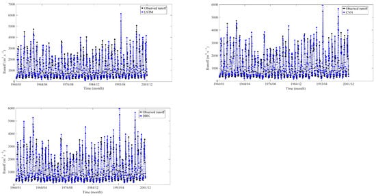
Figure 12.
Training results at JP hydrological station.
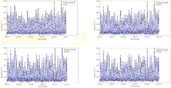
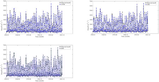
Figure 13.
Training results at GD hydrological station.
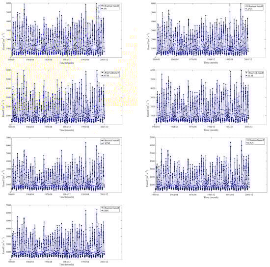
Figure 14.
Training results at ET hydrological station.
Table 4.
Performance comparison of the seven models based on the training results at different stations.
Based on the findings presented in Figure 11, Figure 12, Figure 13 and Figure 14 and Table 4, it is clear that the seven models demonstrate distinct performance characteristics during the training experiments. The training results revealed that the DL models (LSTM, CNN, DBN) demonstrated the best performance in terms of MAPE, RMSE, NSE, and R2.
4.5. Monthly Runoff Validation Results
In the validation analysis experiments, the monthly runoff validation results are shown in Figure 15, Figure 16, Figure 17 and Figure 18. Performance comparison of the seven models based on the validation results at different stations are shown in Table 5.
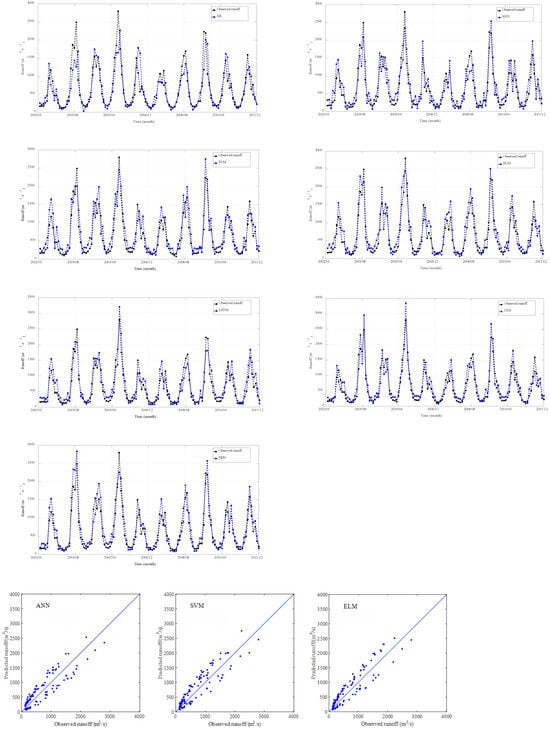
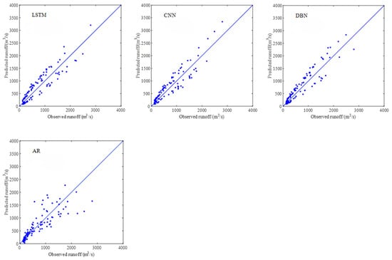
Figure 15.
Validation results obtained using different models at LHK hydrological station.
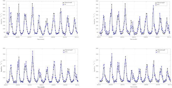
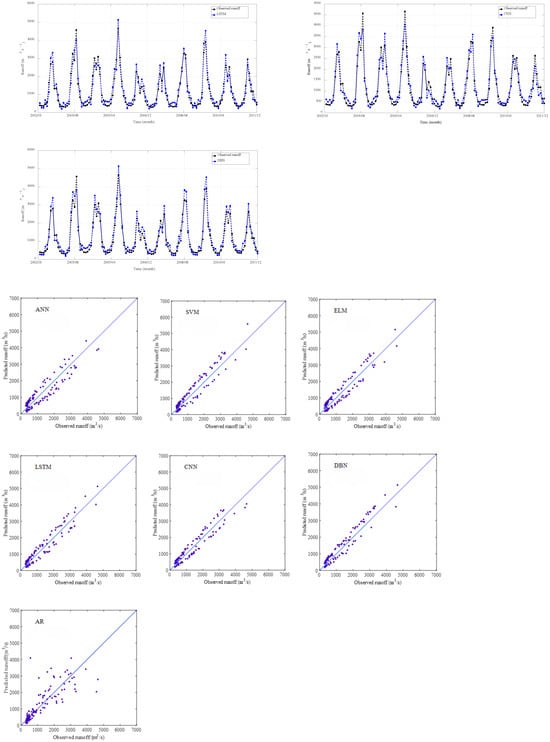
Figure 16.
Validation results obtained using different models at JP hydrological station.
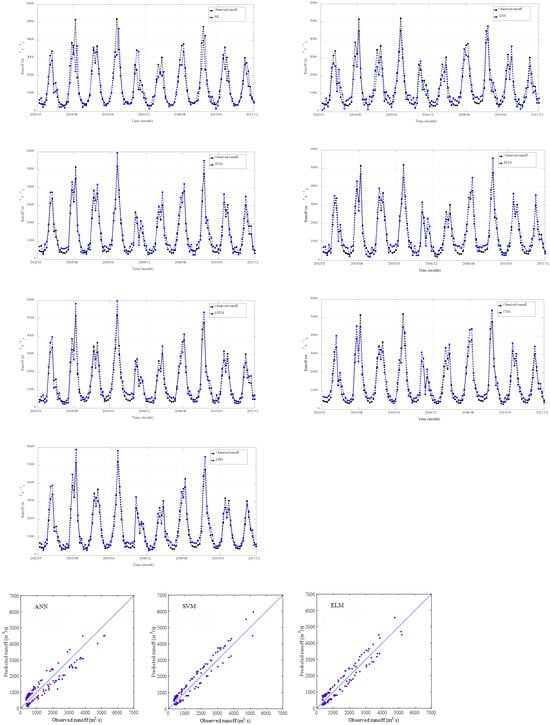
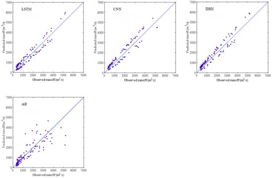
Figure 17.
Validation results obtained using different models at GD hydrological station.
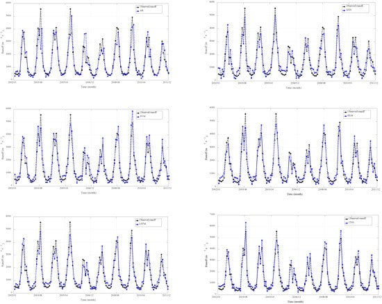
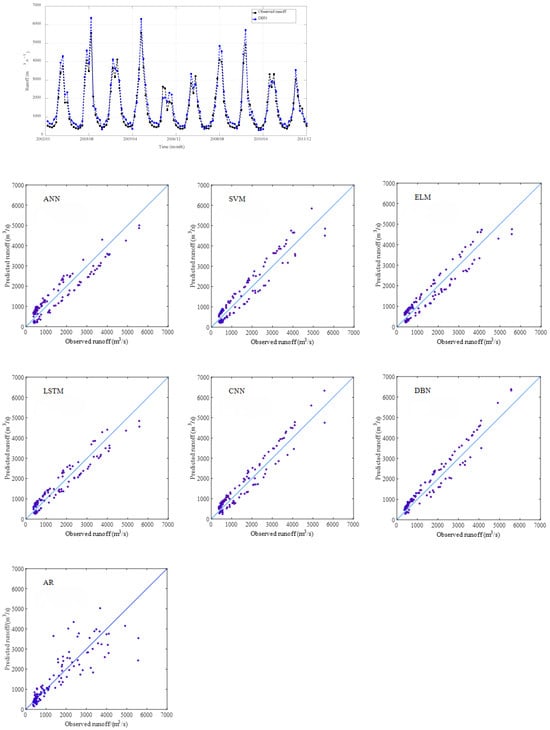
Figure 18.
Validation results obtained using different models at ET hydrological station.
Table 5.
Performance comparison of the seven models based on the validation results at different stations.
Based on the validation results presented in Figure 15, Figure 16, Figure 17 and Figure 18, we can see that all the data-driven models achieved high accuracy in monthly runoff simulation, accurately capturing both the trends and magnitudes of the observed runoff hydrographs across the studied catchments. Therefore, the machine learning methods may adapt effectively to the nonlinear characteristics of runoff series and obtain better simulation effects, especially deep learning models (i.e., LSTM, CNN, and DBN) in terms of MAPE, RMSE, NSE, and R2.
5. Discussion
Hydrologic models are critical computational tools for simulating extreme hydrological events (e.g., floods and droughts) and optimizing integrated water resources management. The PDMs from the classical bucket model are often referred to as conceptual, mechanistic, or process-oriented models. In contrast, the DDMs evolved from traditional statistical analysis based on mathematical regression techniques, with recent advancements focusing on leveraging sophisticated computational intelligence methods. Nevertheless, it remains unclear whether DDMs will progressively dominate over PDMs or the other way around. Additionally, given the different philosophies underlying these two model categories, it is uncertain how traditional PDMs will evolve further.
Aiming to compare the shallow and deep learning-based DDMs for monthly runoff simulation in the YRB, we comparatively investigated the applicability of ANN, SVM, ELM, LSTM, CNN, DBN, and AR models for monthly runoff simulation. In addition, four evaluation indicators, including MAPE, RMSE, NSE, and R2, were employed to verify the performance of the above methods. The results revealed that DDMs demanded limited data and could offer satisfactory simulation effects. Also, the deep learning models outperformed the AR model and other DDMs in terms of the above evaluation criteria. Performance comparison of the seven models based on the validation results at different stations are shown in Table 5.
As shown in Table 5, the comprehensive performance of DBN model (MAPE = 33.62%, RMSE = 224.65 m3/s, NSE = 0.8496, and R2 = 0.8836) was better than other models at LHK hydrological station. The CNN (MAPE = 30.00%, RMSE = 298.51 m3/s, NSE = 0.9135, and R2 = 0.9146) and DBN (MAPE = 29.56%, RMSE = 306.51 m3/s, NSE = 0.9088, and R2 = 0.9396) models were better than other models at JP hydrological station. The comprehensive performance of the LSTM (MAPE = 29.60%, RMSE = 334.56 m3/s, NSE = 0.9197, and R2 = 0.9242) and DBN (MAPE = 28.67%, RMSE = 336.91 m3/s, NSE = 0.9185, and R2 = 0.9371) models were better than other models at GD hydrological station. The simulation effects of the LSTM, CNN, and DBN models were better than the shallow data-driven models (ANN, SVM, ELM) and AR model at ET hydrological station. Consequently, the DDMs could better simulate the relationship between input factors and output runoff data without regard to complex and unknown runoff production and acquire satisfactory simulation results in the YRB.
The AR model may slightly outperform some data-driven models in the MAPE indicator at LHK, GD, and ET hydrological stations in the YRB, but the comprehensive performance of deep learning models significantly outperformed the shallow data-driven models and the AR model in terms of the above evaluation criteria; the AR or shallow models had shallow model structure, the parameters of models need to be initialized, optimized constantly, and could not acquire accurate runoff simulation results. On the contrary, the deep learning-based DDMs (LSTM, CNN, DBN) could calculate via layer-by-layer transmission to learn too many intrinsic characteristics. The deep learning-based models could compensate for the shortcomings of shallow DDMs and enhance the runoff simulation accuracy, speed, and robustness.
In addition, the seven models demonstrated better simulation results for the JP, GD, and ET hydrological stations compared to that of the LHK hydrological station in terms of the MAPE, NSE, and R2 indicators. This might be because the small hydropower stations’ regulation operation in the interval had changed the natural water flow process, thereby reducing the simulation accuracy of the LHK hydrological station. Apart from this, the RMSE indicator is closely related to the annual water volume of the study area. When the flow has large annual water volume, the RMSE index of the domain is also relatively large. In this study, the RMSEs of models were the smallest at LHK, compared with JP, GD, and ET hydrological stations, because the annual water volume of LHK hydrological station was relatively low; thereby the statistical measures (e.g., Min., Max., Ave., and Stdev.) of the runoff data were the smallest.
The experimental results showed that factors selection affected the accuracy of monthly runoff simulation. The key factors were the lag time of 1 month of the North American Polar Vortex Intensity Index (3, 120° W-30° W), 6 months of the Tibet Plateau Region Index (25° N-35° N, 80° E-100° E), 12 months of the Asia Polar Vortex Intensity Index (1, 60° E-150° E), 12 months of the Tibet Plateau Region Index (30° N-40° N, 75° E-105° E), 1 and 12 months of the antecedent runoff, and 1 month of the antecedent area rainfall in LHK hydrological station.
Likewise, the key factors of JP hydrological station were the lag time of 1 month of the North African–North Atlantic–North American Subtropical High Intensity Index (110° W-60° E), 6 months of the Tibet Plateau Region Index (25° N-35° N, 80° E-100° E), 6 and 12 months of the Tibet Plateau Region Index (30° N-40° N, 75° E-105° E), 1 month of the antecedent runoff, and 1 and 12 months of the antecedent area rainfall.
In GD hydrological station, the key factors were the lag time of 1 month of the North African–North Atlantic–North American Subtropical High Intensity Index (110° W-60° E), 1 month of the North American–North Atlantic Subtropical High Intensity Index (110° W-20° W), 7 months of the Tibet Plateau Region Index (25° N-35° N, 80° E-100° E), 8 months of the Asia Polar Vortex Intensity Index (1, 60° E-150° E), 8 months of the Northern Hemisphere Polar Vortex Intensity Index (5, 0–360), 12 months of the Tibet Plateau Region Index (30° N-40° N, 75° E-105° E), 1 month of the antecedent runoff, and 1 and 12 months of the antecedent area rainfall.
In ET hydrological station, the key factors were the lag time of 7 months of the Tibet Plateau Region Index (25° N-35° N, 80° E-100° E), 7 months of the Tibet Plateau Region Index (30° N-40° N, 75° E-105° E), 8 months of the Asia Polar Vortex Intensity Index (1, 60° E-150° E), 8 months of the Northern Hemisphere Polar Vortex Intensity Index (5, 0–360), 1 month of the antecedent runoff, and 1 month of the antecedent area rainfall.
6. Conclusions
In general, it is a great challenge to obtain accurate monthly runoff simulation results, because of the randomness, uncertainty, and complex nonlinear characteristics of runoff time series. Aiming to compare the effectiveness of different models for runoff simulation, we comparatively investigated the applicability of the shallow DDMs, deep learning-based (DL) models, and AR model for monthly runoff simulation at LHK, JP, GD, and ET hydrological stations in the YRB, respectively. Runoff, rainfall, and 95 teleconnection climate factors with Pearson’s correlation coefficient and stepwise regression analysis methods were applied to select input factors as input of DDMs. In addition, four evaluation indicators, including MAPE, RMSE, NSE, and R2, were employed to evaluate the runoff simulation effects of the above methods. Drawing upon the results, the key findings of this paper are as follows:
(1) Factors selection is critical for monthly runoff simulation. The previous runoff, area rainfall, North African–North Atlantic–North American Subtropical High Intensity Index (110° W-60° E), North American–North Atlantic Subtropical High Intensity Index (110° W-20° W), Asia Polar Vortex Intensity Index (1, 60° E-150° E), North American Polar Vortex Intensity Index (3, 120° W-30° W), Northern Hemisphere Polar Vortex Intensity Index (5, 0–360), Tibet Plateau Region Index (25° N-35° N, 80° E-100° E), and Tibet Plateau Region Index (30° N-40° N, 75° E-105° E) are key factors at the four hydrological stations in the YRB.
(2) The DDMs demand limited data and can offer satisfactory prediction effects. Also, the DL models outperform other shallow DDMs and the AR model in terms of the four evaluation criteria.
(3) The runoff simulation results of different data-driven models could provide references for water resources planning and development projects in the Yalong River basin.
We acknowledge that some factors, such as vegetation, soil characteristics, and human activities (operation of dams, irrigation, land use changes) are not considered in this study; we will investigate more factors and recent data for runoff simulation in our future work. In addition, we will conduct research on the development of more efficient multiparameter optimization methods (e.g., Bayesian optimization, cross-validation with grid search, particle swarm optimization, genetic algorithm, artificial bee colony, flower pollination algorithm, and firefly algorithm) based on bio-inspired algorithms for determining the optimal parameters of the data-driven models in our future work. Apart from this, the future work also includes integrating hydrological models with deep learning models via bio-inspired algorithms for runoff simulation.
Author Contributions
Conceptualization, Z.Y.; Data curation, L.W. and J.Z.; Formal analysis, L.W. and J.Z.; Methodology, Z.Y.; Software, Z.Y. and L.W.; Validation, L.W. and J.Z.; Writing—original draft, Z.Y.; Writing—review and editing, Z.Y. and H.Z. All authors have read and agreed to the published version of the manuscript.
Funding
This research was funded by ‘the Industry-University-Research Collaboration Project of Jiangsu Province, (Grant No. BY20230703)’, ‘the Open Foundation of Industrial Perception and Intelligent Manufacturing Equipment Engineering Research Center of Jiangsu Province (Grant No. ZK22-05-13)’, ‘the Natural Science Foundation of Jiangsu Province’ (Grant No. BK20241070), ‘the Natural Science Foundation of the Jiangsu Higher Education Institutions of China’ (Grant No. 24KJD510005), ‘the Start-up Fund for New Talented Researchers of Nanjing University of Industry Technology’ (Grant No. YK24-05-02) and ‘the Research Center of Intelligent Sensor and Network Engineering Technology of Jiangsu Province’ (Grant No. ZK21-05-09).
Data Availability Statement
Hydrological time series data, including daily runoff records, were sourced from the Hydrological Bureau of the Changjiang Water Resources Commission under China’s Ministry of Water Resources (accessible at http://www.cjh.com.cn). Concurrently, climate datasets encompassing atmospheric circulation factors and meteorological data were acquired through the National Climate Center’s open-data portal (http://data.cma.cn).
Conflicts of Interest
The authors declare no conflicts of interest.
References
- Tan, Q.F.; Lei, X.H.; Wang, X.; Wang, H.; Wen, X.; Ji, Y.; Kang, A.Q. An adaptive middle and long-term runoff forecast model using EEMD-ANN hybrid approach. J. Hydrol. 2018, 567, 767–780. [Google Scholar] [CrossRef]
- Yue, Z.; Ai, P.; Xiong, C.; Hong, M.; Song, Y. Mid-to long-term runoff prediction by combining the deep belief network and partial least-squares regression. J. Hydroinform. 2020, 22, 1283–1305. [Google Scholar] [CrossRef]
- Yue, Z.; Ai, P.; Yuan, D.; Xiong, C. Ensemble approach for mid-long term runoff forecasting using hybrid algorithms. J. Ambient Intell. Humaniz. Comput. 2020, 13, 5103–5122. [Google Scholar] [CrossRef]
- Barge, J.T.; Sharif, H.O. An Ensemble Empirical Mode Decomposition, Self-Organizing Map, and Linear Genetic Programming Approach for Forecasting River Streamflow. Water 2016, 8, 247. [Google Scholar] [CrossRef]
- Yue, Z.; Liu, H.; Zhou, H. Monthly Runoff Forecasting Using Particle Swarm Optimization Coupled with Flower Pollination Algorithm-Based Deep Belief Networks: A Case Study in the Yalong River Basin. Water 2023, 15, 2704. [Google Scholar] [CrossRef]
- Tripathy, K.P.; Mishra, A.K. Deep learning in hydrology and water resources disciplines: Concepts, methods, applications, and research directions. J. Hydrol. 2024, 628, 130458. [Google Scholar] [CrossRef]
- Islam, Z. A Review on Physically Based Hydrologic Modeling; University of Alberta: Edmonton, AB, Canada, 2011. [Google Scholar]
- Kim, T.; Yang, T.; Gao, S.; Zhang, L.; Ding, Z.; Wen, X.; Gourley, J.J.; Hong, Y. Can artificial intelligence and data-driven machine learning models match or even replace process-driven hydrologic models for streamflow simulation?: A case study of four watersheds with different hydro-climatic regions across the CONUS. J. Hydrol. 2021, 598, 126423. [Google Scholar] [CrossRef]
- Jiang, Z.; Lu, B.; Zhou, Z.; Zhao, Y. Comparison of Process-Driven SWAT Model and Data-Driven Machine Learning Techniques in Simulating Streamflow: A Case Study in the Fenhe River Basin. Sustainability 2024, 16, 6074. [Google Scholar] [CrossRef]
- Sorooshian, S.; Duan, Q.; Gupta, V.K. Calibration of rainfall-runoff models: Application of global optimization to the Sacramento Soil Moisture Accounting Model. Water Resour. Res. 1993, 29, 1185–1194. [Google Scholar] [CrossRef]
- Moreda, F.; Koren, V.; Zhang, Z.; Reed, S.; Smith, M. Parameterization of distributed hydrological models: Learning from the experiences of lumped modeling. J. Hydrol. 2006, 320, 218–237. [Google Scholar] [CrossRef]
- Behrangi, A.; Khakbaz, B.; Jaw, T.C.; AghaKouchak, A.; Hsu, K.; Sorooshian, S. Hydrologic evaluation of satellite precipitation products over a mid-size basin. J. Hydrol. 2011, 397, 225–237. [Google Scholar] [CrossRef]
- Chu, W.; Gao, X.; Sorooshian, S. Improving the shuffled complex evolution scheme for optimization of complex nonlinear hydrological systems: Application to the calibration of the Sacramento soil moisture accounting model. Water Resour. Res. 2010, 46. [Google Scholar] [CrossRef]
- Zhao, R.; Liu, X. The Xinanjiang Model, Computer Models of Watershed Hydrology; Singh, V.P., Ed.; Water Resources Publications: California City, CA, USA, 1995; pp. 215–232. [Google Scholar]
- Xu, H.; Xu, C.Y.; Chen, H.; Zhang, Z.; Li, L. Assessing the influence of rain gauge density and distribution on hydrological model performance in a humid region of China. J. Hydrol. 2013, 505, 1–12. [Google Scholar] [CrossRef]
- Zeng, Q.; Chen, H.; Xu, C.Y.; Jie, M.-X.; Chen, J.; Guo, S.-L.; Liu, J. The effect of rain gauge density and distribution on runoff simulation using a lumped hydrological modelling approach. J. Hydrol. 2018, 563, 106–122. [Google Scholar] [CrossRef]
- Fang, Y.H.; Zhang, X.; Corbari, C.; Mancini, M.; Niu, G.-Y.; Zeng, W. Improving the Xin’anjiang hydrological model based on mass–energy balance. Hydrol. Earth Syst. Sci. 2017, 21, 3359–3375. [Google Scholar] [CrossRef]
- Xu, D.; Wang, W.; Chau, K.; Cheng, C.-T.; Chen, S.-Y. Comparison of three global optimization algorithms for calibration of the Xinanjiang model parameters. J. Hydroinform. 2013, 15, 174–193. [Google Scholar] [CrossRef]
- Sheng, Z.; Wen, S.; Feng, Z.K.; Gong, J.; Shi, K.; Guo, Z.; Yang, Y.; Huang, T. A survey on data-driven runoff forecasting models based on neural networks. IEEE Trans. Emerg. Top. Comput. Intell. 2023, 7, 1083–1097. [Google Scholar] [CrossRef]
- Mohammadi, B. A review on the applications of machine learning for runoff modeling. Sustain. Water Resour. Manag. 2021, 7, 98. [Google Scholar] [CrossRef]
- Yazdani, M.R.; Saghafian, B.; Mahdian, M.H.; Soltani, S. Monthly runoff estimation using artificial neural networks. J. Agric. Sci. Technol. 2009, 11, 335–362. [Google Scholar]
- Samantaray, S.; Das, S.S.; Sahoo, A.; Satapathy, D.P. Monthly runoff prediction at Baitarani river basin by support vector machine based on Salp swarm algorithm. Ain Shams Eng. J. 2022, 13, 101732. [Google Scholar] [CrossRef]
- Yaseen, Z.M.; Jaafar, O.; Deo, R.C.; Kisi, O.; Adamowski, J.; Quilty, J.; El-Shafie, A. Stream-flow forecasting using extreme learning machines: A case study in a semi-arid region in iraq. J. Hydrol. 2016, 542, 603–614. [Google Scholar] [CrossRef]
- He, C.; Chen, F.; Long, A.; Qian, Y.; Tang, H. Improving the precision of monthly runoff prediction using the combined non-stationary methods in an oasis irrigation area. Agric. Water Manag. 2023, 279, 108161. [Google Scholar] [CrossRef]
- Li, X.; Zhang, L.; Zeng, S.; Tang, Z.; Liu, L.; Zhang, Q.; Tang, Z.; Hua, X. Predicting Monthly Runoff of the Upper Yangtze River Based on Multiple Machine Learning Models. Sustainability 2022, 14, 11149. [Google Scholar] [CrossRef]
- Sit, M.A.; Demiray, B.Z.; Xiang, Z.; Ewing, G.; Sermet, Y.; Demir, I. A comprehensive review of deep learning applications in hydrology and water resources. Water Sci. Technol. 2020, 82, 2635–2670. [Google Scholar] [CrossRef]
- Van, S.P.; Le, H.M.; Thanh, D.V.; Dang, T.D.; Loc, H.H.; Anh, D.T. Deep learning convolutional neural network in rainfall–runoff modelling. J. Hydroinform. 2020, 22, 541–561. [Google Scholar] [CrossRef]
- Wang, W.C.; Wang, B.; Chau, K.W.; Xu, D.M. Monthly runoff time series interval prediction based on WOA-VMD-LSTM using non-parametric kernel density estimation. Earth Sci. Inform. 2023, 16, 2373–2389. [Google Scholar] [CrossRef]
- Jain, A.; Mao, J.; Mohiuddin, K. Artificial neural networks: A tutorial. Computer 1996, 29, 31–44. [Google Scholar] [CrossRef]
- Haykin, S.; Network, N. A comprehensive foundation. Neural Netw. 2004, 2, 41. [Google Scholar]
- Huang, G.B.; Zuo, B.; Gong, W.Y.; Kasun, L.L.C.; Vong, C.M. Local receptive fields based extreme learning machine. IEEE Comput. Intell. Mag. 2015, 10, 18–29. [Google Scholar] [CrossRef]
- Yaseen, Z.M.; Sulaiman, S.O.; Deo, R.C.; Chau, K.-W. An enhanced extreme learning machine model for river flow forecasting: State-of-the-art, practical applications in water resource engineering area and future research direction. J. Hydrol. 2018, 569, 387–408. [Google Scholar] [CrossRef]
- Schmidhuber, J.; Hochreiter, S. Long short-term memory. Neural Comput. 1997, 9, 1735–1780. [Google Scholar] [CrossRef]
- Kratzert, F.; Klotz, D.; Brenner, C.; Schulz, K.; Herrnegger, M. Rainfall–runoff modelling using long short-term memory (LSTM) networks. Hydrol. Earth Syst. Sci. 2018, 22, 6005–6022. [Google Scholar] [CrossRef]
- Zhang, J.; Chen, X.; Khan, A.; Zhang, Y.-K.; Kuang, X.; Liang, X.; Taccari, M.L.; Nuttall, J. Daily runoff forecasting by deep recursive neural network. J. Hydrol. 2021, 596, 126067. [Google Scholar] [CrossRef]
- Wen, L.; Li, X.; Gao, L.; Zhang, Y. A New Convolutional Neural Network Based Data-Driven Fault Diagnosis Method. IEEE Trans. Ind. Electron. 2018, 65, 5990–5998. [Google Scholar] [CrossRef]
- Schmidhuber, J. Deep Learning in Neural Networks: An Overview. Neural Netw. 2015, 61, 85–117. [Google Scholar] [CrossRef]
- Shu, X.; Ding, W.; Peng, Y.; Wang, Z.; Wu, J.; Li, M. Monthly Streamflow Forecasting Using Convolutional Neural Network. Water Resour. Manag. 2021, 35, 5089–5104. [Google Scholar] [CrossRef]
- Yang, X.; Zhang, X.; Xie, J.; Zhang, X.; Liu, S. Monthly Runoff Interval Prediction Based on Fuzzy Information Granulation and Improved Neural Network. Water 2022, 14, 3683. [Google Scholar] [CrossRef]
- Yuan, X.; Chen, C.; Lei, X.; Yuan, Y.; Muhammad Adnan, R. Monthly runoff forecasting based on LSTM–ALO model. Stoch. Environ. Res. Risk Assess. 2018, 32, 2199–2212. [Google Scholar] [CrossRef]
- Ai, P.; Song, Y.; Xiong, C.; Chen, B.; Yue, Z. A novel medium-and long-term runoff combined forecasting model based on different lag periods. J. Hydroinform. 2022, 24, 367–387. [Google Scholar] [CrossRef]
- Erdem, O.; Ceyhan, E.; Varli, Y. A new correlation coefficient for bivariate time-series data. Phys. A Stat. Mech. Its Appl. 2014, 414, 274–284. [Google Scholar] [CrossRef]
- Deng, W.; Yao, R.; Zhao, H.; Yang, X.; Li, G. A novel intelligent diagnosis method using optimal LS-SVM with improved PSO algorithm. Soft Comput. 2019, 23, 2445–2462. [Google Scholar] [CrossRef]
Disclaimer/Publisher’s Note: The statements, opinions and data contained in all publications are solely those of the individual author(s) and contributor(s) and not of MDPI and/or the editor(s). MDPI and/or the editor(s) disclaim responsibility for any injury to people or property resulting from any ideas, methods, instructions or products referred to in the content. |
© 2025 by the authors. Licensee MDPI, Basel, Switzerland. This article is an open access article distributed under the terms and conditions of the Creative Commons Attribution (CC BY) license (https://creativecommons.org/licenses/by/4.0/).