Groundwater Level Trend Analysis and Prediction in the Upper Crocodile Sub-Basin, South Africa

 , ,
, ,  and
and
Abstract
:1. Introduction
2. Materials and Methods
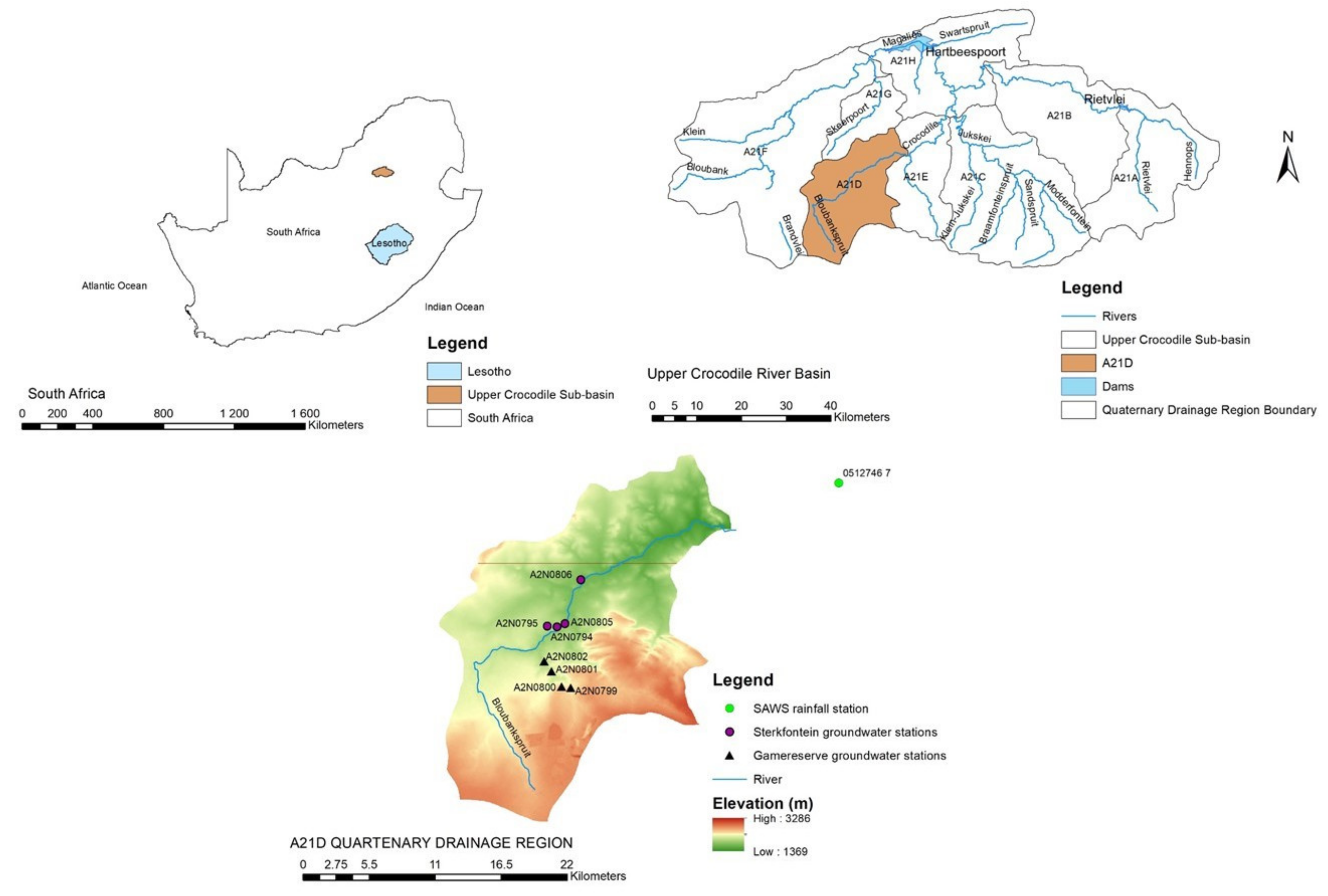
2.1. Study Area Description
2.2. Data Sources and Acquisition
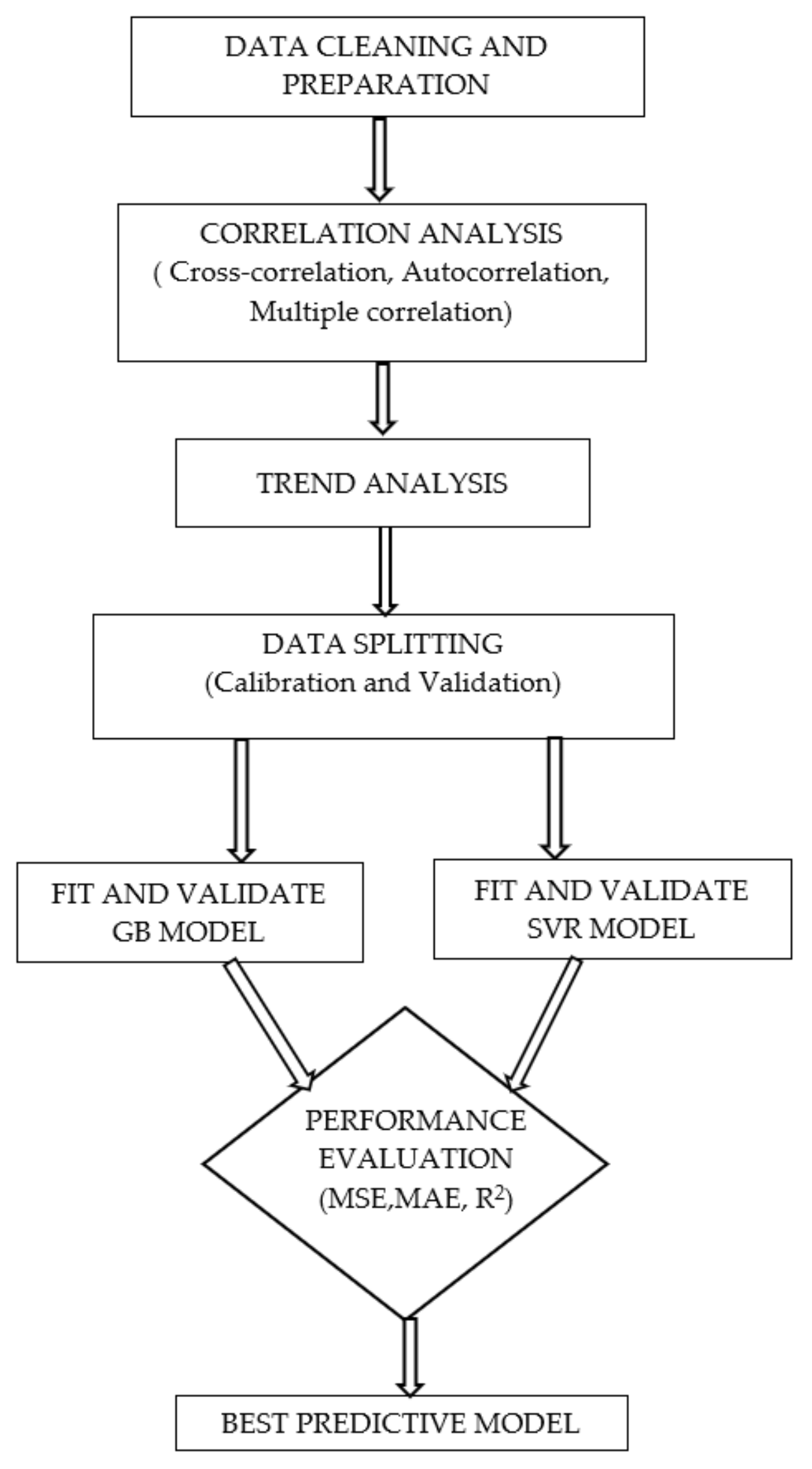
2.3. Methods
2.3.1. Correlation Analysis
- (a)
- Cross correlation analysis
- (b)
- Autocorrelation Analysis
- (c)
- Multiple correlation analysis
2.3.2. Trend Analysis
2.3.3. Gradient Boosting Regression
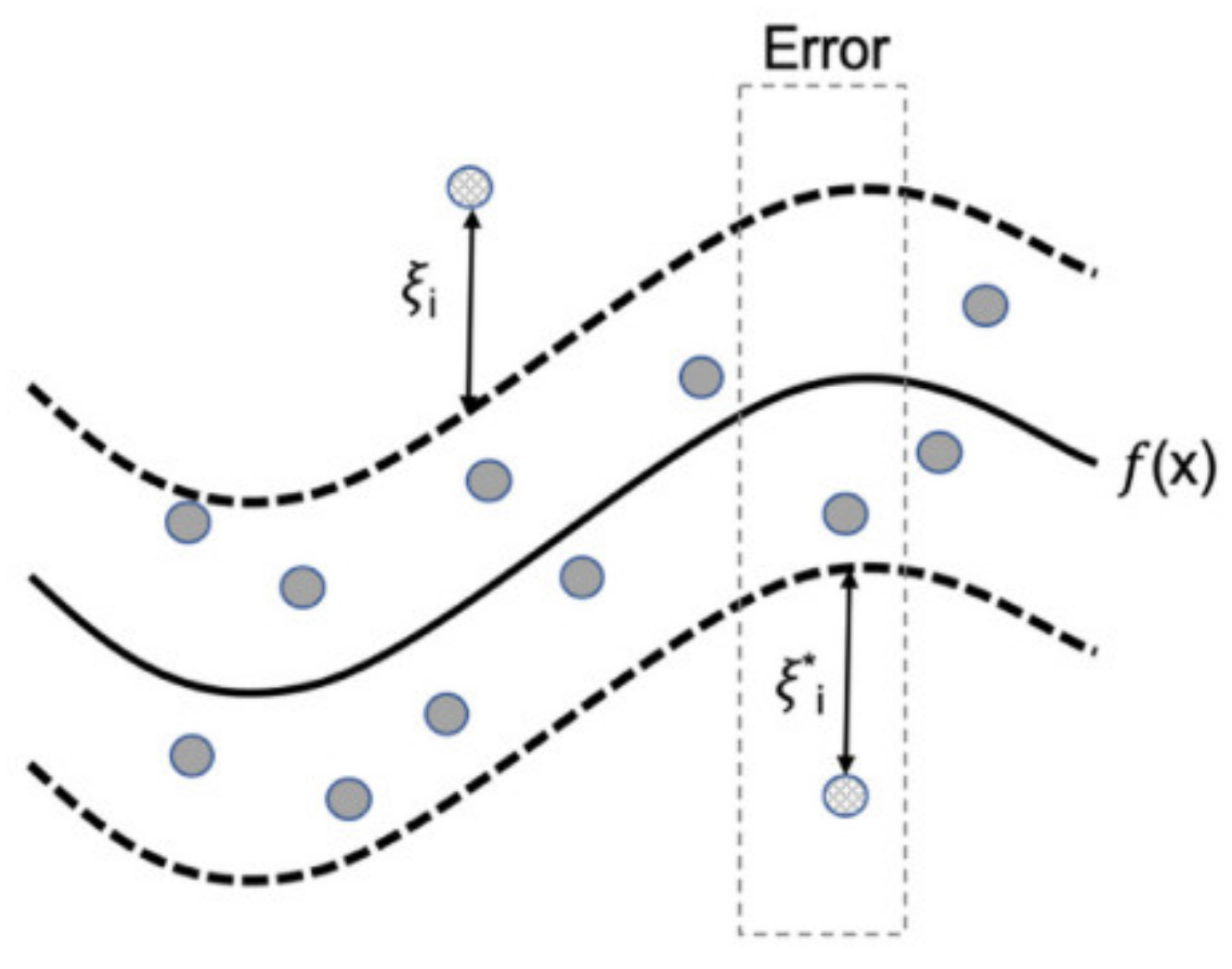
2.3.4. Support Vector Regression
2.3.5. Performance Evaluation of Predictive Models
3. Results and Discussions
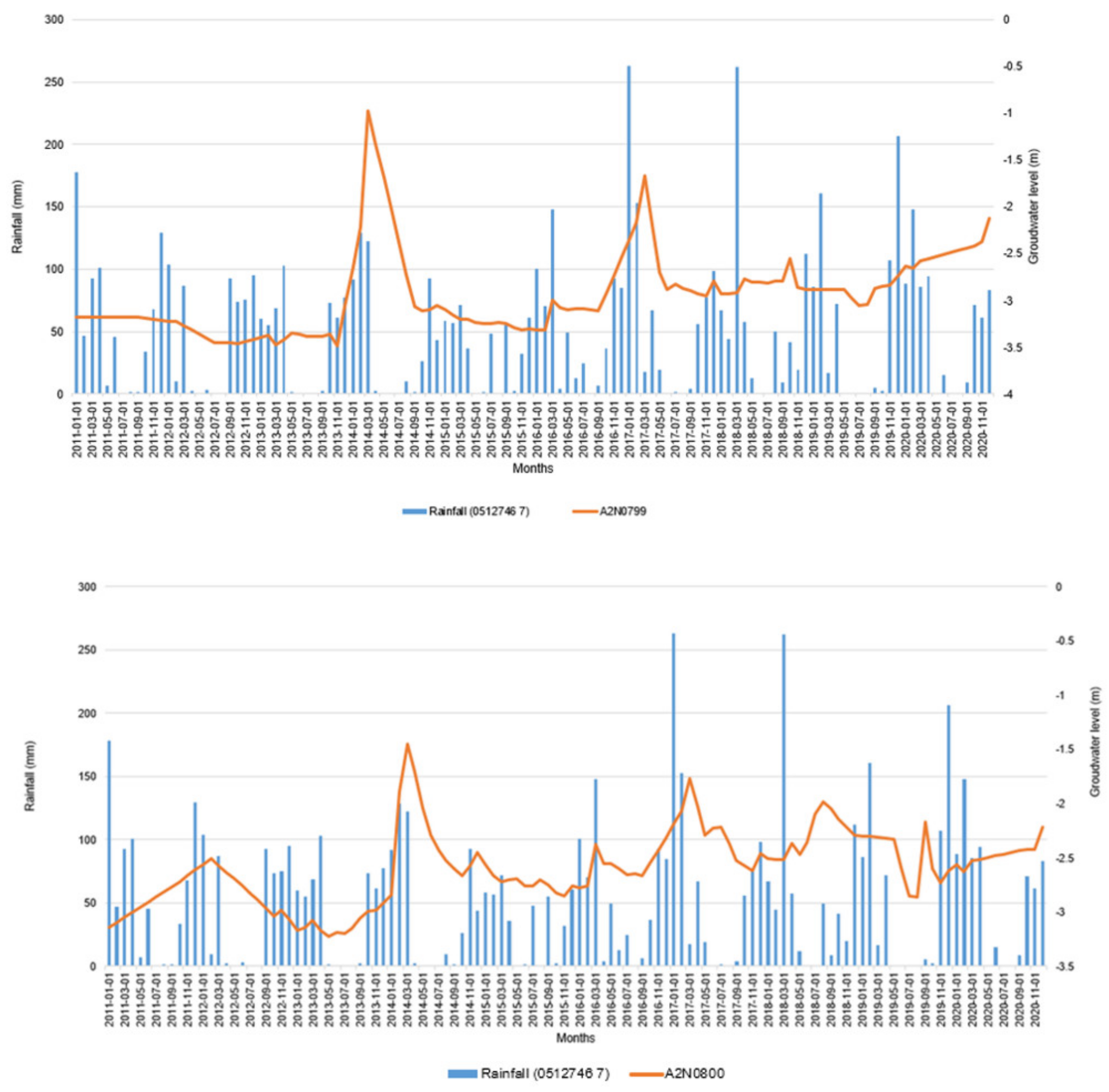
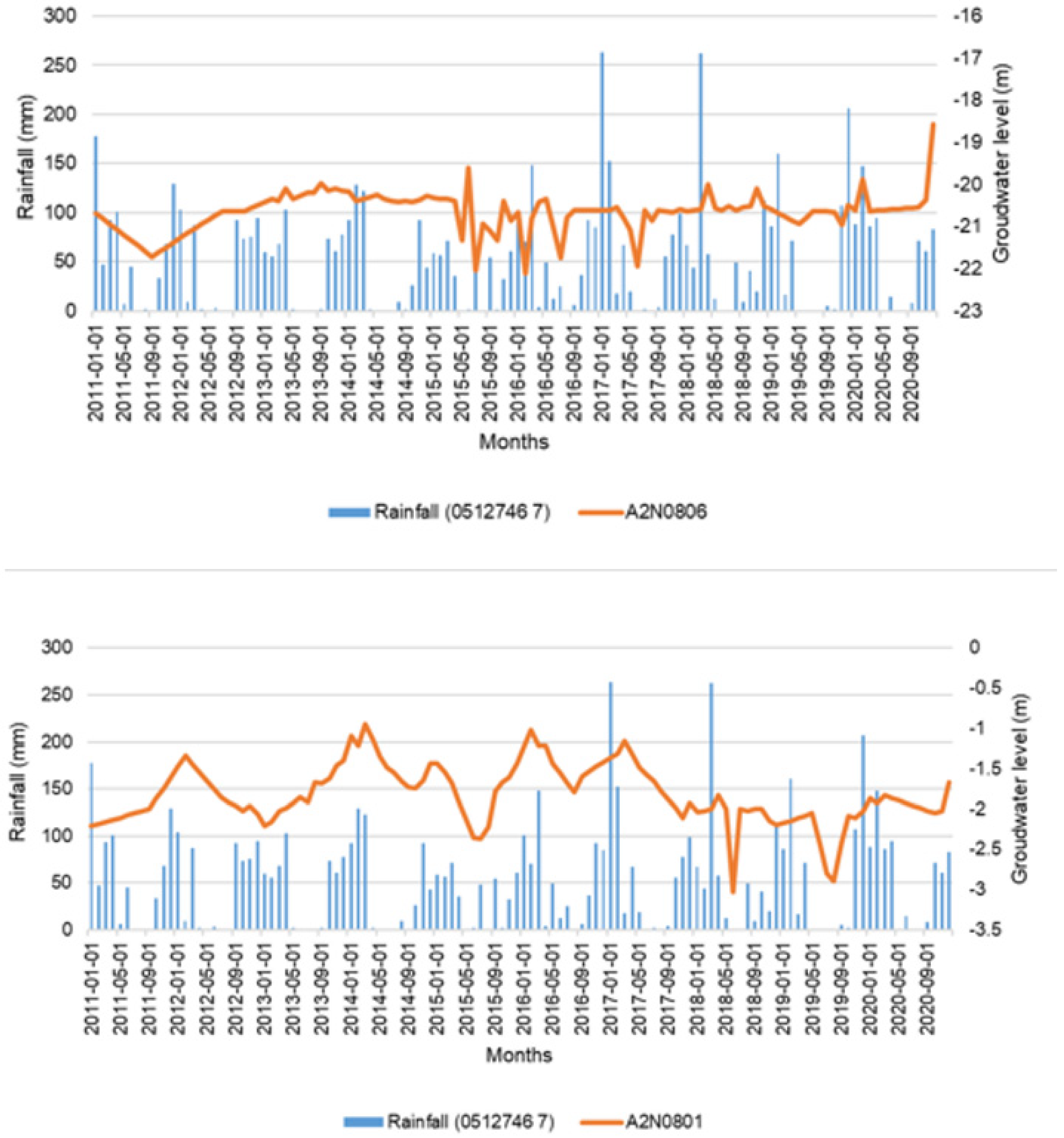
3.1. Correlation Analysis
3.2. Trend Analysis
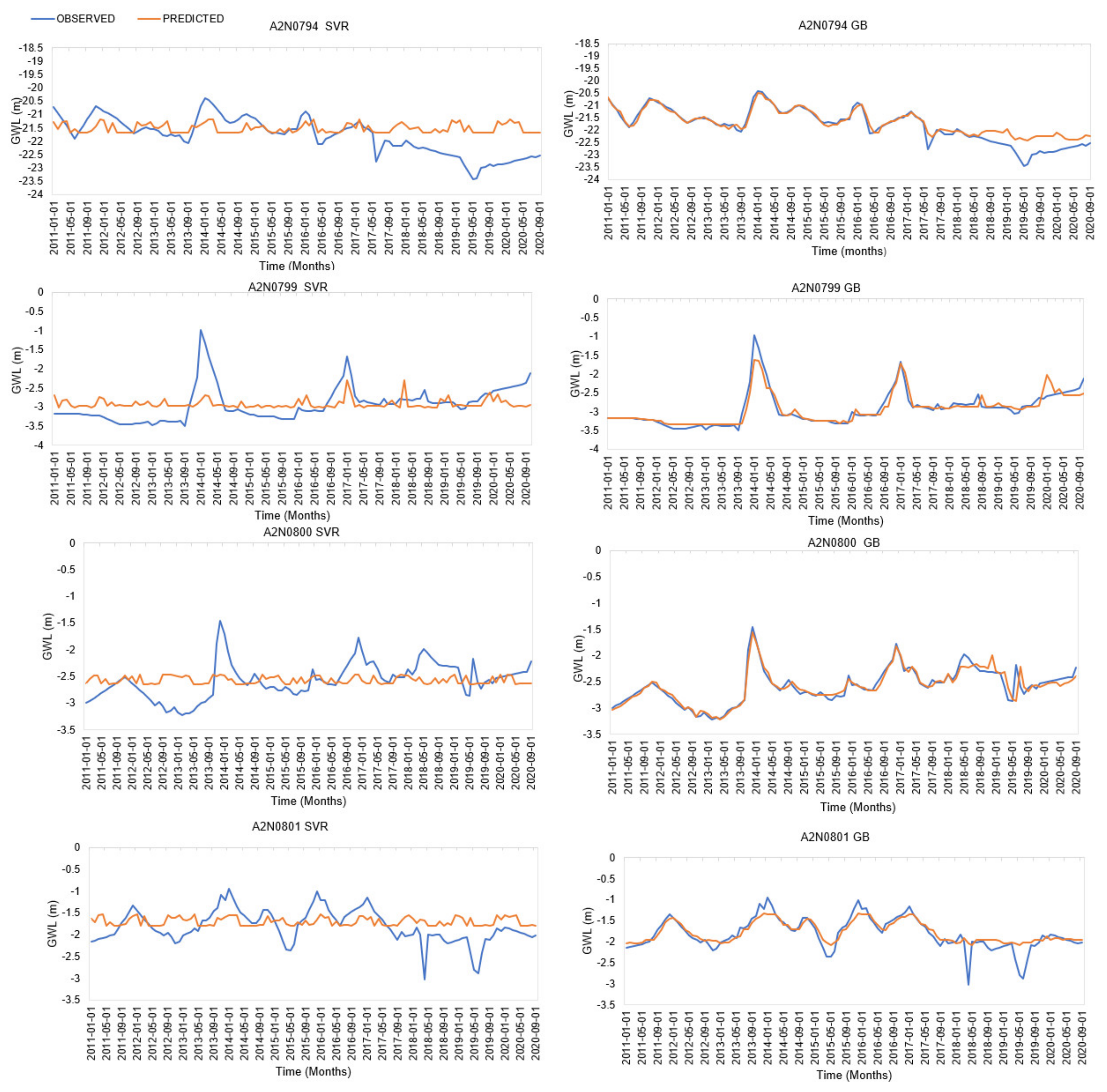
3.3. Performance Evaluation of the Predictive Model
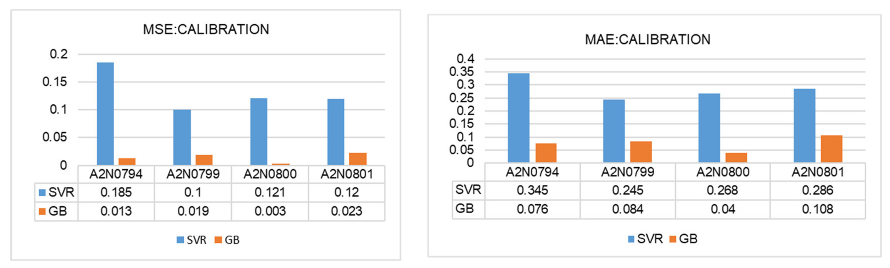
3.3.1. MSE and MAE
3.3.2. Scatterplot Analysis
4. Conclusions and Recommendations
Author Contributions
Funding
Data Availability Statement
Acknowledgments
Conflicts of Interest
References
- Ziervogel, G.; New, M.; Archer van Garderen, E.; Midgley, G.; Taylor, A.; Hamann, R.; Stuart-Hill, S.; Myers, J.; Warburton, M. Climate change impacts and adaptation in South Africa. Wiley Interdiscip. Rev. Clim. Change 2014, 5, 605–620. [Google Scholar] [CrossRef]
- IPCC. Climate Change 2014: Impacts, Adaptation, and Vulnerability. Part A: Global and Sectoral Aspects. Contribution of Working Group II to the Fifth Assessment Report of the Intergovernmental Panel on Climate Change; Intergovernmental Panel on Climate Change: New York, NY, USA, 2014. [Google Scholar]
- Mishra, A.K.; Singh, V.P. A review of drought concepts. J. Hydrol. 2010, 391, 202–216. [Google Scholar] [CrossRef]
- Wanders, N.; Wada, Y.; Van Lanen, H.A.J. Global hydrological droughts in the 21st century under a changing hydrological regime. Earth Syst. Dyn. 2015, 6, 1–15. [Google Scholar] [CrossRef]
- Prodhan, F.A.; Zhang, J.; Pangali Sharma, T.P.; Nanzad, L.; Zhang, D.; Seka, A.M.; Ahmed, N.; Hasan, S.S.; Hoque, M.Z.; Mohana, H.P. Projection of future drought and its impact on simulated crop yield over South Asia using ensemble machine learning approach. Sci. Total Environ. 2022, 807, 151029. [Google Scholar] [CrossRef]
- Dilawar, A.; Chen, B.; Arshad, A.; Guo, L.; Ehsan, M.I.; Hussain, Y.; Kayiranga, A.; Measho, S.; Zhang, H.; Wang, F.; et al. Towards understanding variability in droughts in response to extreme climate conditions over the different agro-ecological zones of Pakistan. Sustainability 2021, 13, 6910. [Google Scholar] [CrossRef]
- Centre for Research on the Epidemiology of Disasters. Disasters in Numbers 2022; CRED: Brussels, Belgium, 2023. [Google Scholar]
- Schreiner, B.G.; Mungatana, E.D.; Baleta, H. Impacts of Drought Induced Water Shortages in South Africa: Economic Analysis Report to the Water Research Commission. 2018. Available online: www.wrc.org.za (accessed on 15 February 2023).
- Archer, E.; du Toit, J.; Engelbrecht, C.; Hoffman, M.T.; Landman, W.; Malherbe, J.; Stern, M. The 2015-19 multi year drought in the Eastern Cape, South Africa: It’s evolution and impacts on agriculture. J. Arid Environ. 2022, 196, 104630. [Google Scholar] [CrossRef]
- Holmes, M.; Campbell, E.E.; De Wit, M.; Taylor, J.C. South African Journal of Botany The impact of drought in the Karoo—Revisiting diatoms as water quality indicators in the upper reaches of the Great Fish River, Eastern Cape, South Africa. S. Afr. J. Bot. 2022, 149, 502–510. [Google Scholar] [CrossRef]
- Olanrewaju, C.C.; Reddy, M. Assessment and prediction of flood hazards using standardized precipitation index—A case study of eThekwini metropolitan area. J. Flood Risk Manag. 2022, 15, e12788. [Google Scholar] [CrossRef]
- Bopape, M.J.M.; Sebego, E.; Ndarana, T.; Maseko, B.; Netshilema, M.; Gijben, M.; Landman, S.; Phaduli, E.; Rambuwani, G.; van Hemert, L.; et al. Evaluating south african weather service information on idai tropical cyclone and kwazulu-natal flood events. S. Afr. J. Sci. 2021, 117, 1–13. [Google Scholar] [CrossRef]
- Madzivhandila Thanyani, S.; Maserumule, M.H. The Irony of A “Fire Fighting” Approach Towards Natural Hazards in South Africa: Lessons from Flooding Disaster in KwaZulu-Natal. J. Public Adm. 2022, 57, 191–194. [Google Scholar]
- Chandrasekara, S.S.K.; Kwon, H.H.; Vithanage, M.; Obeysekera, J.; Kim, T.W. Drought in south Asia: A review of drought assessment and prediction in south Asian countries. Atmosphere 2021, 12, 369. [Google Scholar] [CrossRef]
- Hussain, M.; Butt, A.R.; Uzma, F.; Ahmed, R.; Irshad, S.; Rehman, A.; Yousaf, B. A comprehensive review of climate change impacts, adaptation, and mitigation on environmental and natural calamities in Pakistan. Environ. Monit. Assess. 2020, 192, 48. [Google Scholar] [CrossRef] [PubMed]
- Quesada-Román, A.; Villalobos-Portilla, E.; Campos-Durán, D. Hydrometeorological disasters in urban areas of Costa Rica, Central America. Environ. Hazards 2020, 20, 264–278. [Google Scholar] [CrossRef]
- Department of Water Affairs. Groundwater Strategy 2010; Department of Water and Sanitation: Pretoria, South Africa, 2010.
- Pietersen, K.; Beekman, H.E.; Holland, M. South African Groundwater Governance Case Study; WRC: Pretoria, South Africa, 2011. [Google Scholar]
- Bloomfield, J.P.; Allen, D.J.; Griffiths, K.J. Examining geological controls on baseflow index (BFI) using regression analysis: An illustration from the Thames Basin, UK. J. Hydrol. 2009, 373, 164–176. [Google Scholar] [CrossRef]
- Zomlot, Z.; Verbeiren, B.; Huysmans, M.; Batelaan, O. Spatial distribution of groundwater recharge and base flow: Assessment of controlling factors. J. Hydrol. Reg. Stud. 2015, 4, 349–368. [Google Scholar] [CrossRef]
- Mohan, C.; Western, A.W.; Wei, Y.; Saft, M. Predicting groundwater recharge for varying land cover and climate conditions—A global meta-study. Hydrol. Earth Syst. Sci. 2018, 22, 2689–2703. [Google Scholar] [CrossRef]
- Keese, K.E.; Scanlon, B.R.; Reedy, R.C. Assessing controls on diffuse groundwater recharge using unsaturated flow modeling. Water Resour. Res. 2005, 41, 1–12. [Google Scholar] [CrossRef]
- Sun, H.; Cornish, P.S. Estimating shallow groundwater recharge in the headwaters of the Liverpool Plains using SWAT. Hydrol. Process. 2005, 19, 795–807. [Google Scholar] [CrossRef]
- Alfaro, P.; Liesch, T.; Goldscheider, N. Modelling groundwater over-extraction in the southern Jordan Valley with scarce data. Hydrogeol. J. 2017, 25, 1319–1340. [Google Scholar] [CrossRef]
- Oke, S.A.; Fourie, F. Guidelines to groundwater vulnerability mapping for Sub-Saharan Africa. Groundw. Sustain. Dev. 2017, 5, 168–177. [Google Scholar] [CrossRef]
- Sahoo, M.; Kasot, A.; Dhar, A.; Kar, A. On Predictability of Groundwater Level in Shallow Wells Using Satellite Observations. Water Resour. Manag. 2018, 32, 1225–1244. [Google Scholar] [CrossRef]
- Castellazzi, P.; Longuevergne, L.; Martel, R.; Rivera, A.; Brouard, C.; Chaussard, E. Quantitative mapping of groundwater depletion at the water management scale using a combined GRACE/InSAR approach. Remote Sens. Environ. 2018, 205, 408–418. [Google Scholar] [CrossRef]
- Lyazidi, R.; Hessane, M.A.; Moutei, J.F.; Bahir, M. Developing a methodology for estimating the groundwater levels of coastal aquifers in the Gareb-Bourag plains, Morocco embedding the visual MODFLOW techniques in groundwater modeling system. Groundw. Sustain. Dev. 2020, 11, 100471. [Google Scholar] [CrossRef]
- Ostad-Ali-Askari, K.; Ghorbanizadeh Kharazi, H.; Shayannejad, M.; Zareian, M.J. Effect of management strategies on reducing negative impacts of climate change on water resources of the Isfahan–Borkhar aquifer using MODFLOW. River Res. Appl. 2019, 35, 611–631. [Google Scholar] [CrossRef]
- Ibrahem, A.; Osman, A.; Najah, A.; Fai, M.; Feng, Y.; El-Shafie, A. Extreme gradient boosting (Xgboost) model to predict the groundwater levels in Selangor Malaysia. Ain Shams Eng. J. 2021, 12, 1545–1556. [Google Scholar] [CrossRef]
- Malekzadeh, M.; Kardar, S.; Shabanlou, S. Simulation of groundwater level using MODFLOW, extreme learning machine and Wavelet-Extreme Learning Machine models. Groundw. Sustain. Dev. 2019, 9, 100279. [Google Scholar] [CrossRef]
- Zeydalinejad, N. Artificial neural networks vis-à-vis MODFLOW in the simulation of groundwater: A review. Model. Earth Syst. Environ. 2022, 8, 2911–2932. [Google Scholar] [CrossRef]
- Rezaei, M.; Mousavi, S.F.; Moridi, A.; Eshaghi Gordji, M.; Karami, H. A new hybrid framework based on integration of optimization algorithms and numerical method for estimating monthly groundwater level. Arab. J. Geosci. 2021, 14, 994. [Google Scholar] [CrossRef]
- Ahmadi, A.; Olyaei, M.; Heydari, Z.; Emami, M.; Zeynolabedin, A.; Ghomlaghi, A.; Daccache, A.; Fogg, G.E.; Sadegh, M. Groundwater Level Modeling with Machine Learning: A Systematic Review and Meta-Analysis. Water 2022, 14, 949. [Google Scholar] [CrossRef]
- Hussein, E.A.; Thron, C.; Ghaziasgar, M.; Bagula, A.; Vaccari, M. Groundwater prediction using machine-learning tools. Algorithms 2020, 13, 300. [Google Scholar] [CrossRef]
- Sharafati, A.; Asadollah, S.B.H.S.; Neshat, A. A new artificial intelligence strategy for predicting the groundwater level over the Rafsanjan aquifer in Iran. J. Hydrol. 2020, 591, 125468. [Google Scholar] [CrossRef]
- Murdoch, W.J.; Singh, C.; Kumbier, K.; Abbasi-Asl, R.; Yu, B. Definitions, methods, and applications in interpretable machine learning. Proc. Natl. Acad. Sci. USA 2019, 116, 22071–22080. [Google Scholar] [CrossRef] [PubMed]
- Aderemi, B.A.; Olwal, T.O.; Ndambuki, J.M.; Rwanga, S.S. Groundwater levels forecasting using machine learning models: A case study of the groundwater region 10 at Karst Belt, South Africa. Syst. Soft Comput. 2023, 5, 200049. [Google Scholar] [CrossRef]
- Osman, A.I.A.; Ahmed, A.N.; Huang, Y.F.; Kumar, P.; Birima, A.H.; Sherif, M.; Sefelnasr, A.; Ebraheemand, A.A.; El-Shafie, A. Past, Present and Perspective Methodology for Groundwater Modeling-Based Machine Learning Approaches. Arch. Comput. Methods Eng. 2022, 29, 3843–3859. [Google Scholar] [CrossRef]
- Wei, A.; Chen, Y.; Li, D.; Zhang, X.; Wu, T.; Li, H. Prediction of groundwater level using the hybrid model combining wavelet transform and machine learning algorithms. Earth Sci. Inform. 2022, 15, 1951–1962. [Google Scholar] [CrossRef]
- Ouali, L.; Kabiri, L.; Namous, M.; Hssaisoune, M.; Abdelrahman, K.; Fnais, M.S.; Kabiri, H.; El Hafyani, M.; Oubaassine, H.; Arioua, A.; et al. Spatial Prediction of Groundwater Withdrawal Potential Using Shallow, Hybrid, and Deep Learning Algorithms in the Toudgha Oasis, Southeast Morocco. Sustainability 2023, 15, 3874. [Google Scholar] [CrossRef]
- Kanyama, Y.; Ajoodha, R.; Seyler, H.; Makondo, N.; Tutu, H. Application of machine learning techniques in forecasting groundwater levels in the Grootfontein aquifer. In Proceedings of the 2020 2nd International Multidisciplinary Information Technology and Engineering Conference (IMITEC 2020), Kimberley, South Africa, 25–27 November 2020. [Google Scholar] [CrossRef]
- Zhang, Y.; Haghani, A. A gradient boosting method to improve travel time prediction. Transp. Res. Part C 2015, 58, 308–324. [Google Scholar] [CrossRef]
- Jafari, H.; Rajaee, T.; Kisi, O. Improved Water Quality Prediction with Hybrid Wavelet-Genetic Programming Model and Shannon Entropy. Nat. Resour. Res. 2020, 29, 3819–3840. [Google Scholar] [CrossRef]
- He, X.; Luo, J.; Li, P.; Zuo, G.; Xie, J. A Hybrid Model Based on Variational Mode Decomposition and Gradient Boosting Regression Tree for Monthly Runoff Forecasting. Water Resour. Manag. 2020, 34, 865–884. [Google Scholar] [CrossRef]
- An, R.; Tong, Z.; Ding, Y.; Tan, B.; Wu, Z.; Xiong, Q.; Liu, Y. Examining non-linear built environment effects on injurious traffic collisions: A gradient boosting decision tree analysis. J. Transp. Health 2022, 24, 101296. [Google Scholar] [CrossRef]
- Olinsky, A.; Kennedy, B.B. Assessing Gradient Boosting in the Reduction of Misclassification Error in the Prediction of Success for Actuarial Majors. Case Stud. Bus. Ind. Gov. Stat. 2012, 5, 12–16. [Google Scholar]
- Maier, H.R.; Dandy, G.C. Neural networks for the prediction and forecasting of water resources variables: A review of modelling issues and applications. Environ. Model. Softw. 2000, 15, 101–124. [Google Scholar] [CrossRef]
- Tao, H.; Majeed, M.; Abdulameer, H.; Zounemat, M.; Heddam, S.; Kim, S.; Oleiwi, S.; Leong, M.; Sa, Z.; Danandeh, A.; et al. Neurocomputing Groundwater level prediction using machine learning models: A comprehensive review. Neurocomputing 2022, 489, 271–308. [Google Scholar] [CrossRef]
- Derbela, M.; Nouiri, I. Intelligent approach to predict future groundwater level based on artificial neural networks (ANN). Euro-Mediterr. J. Environ. Integr. 2020, 5, 51. [Google Scholar] [CrossRef]
- Yoon, H.; Hyun, Y.; Ha, K.; Lee, K.; Kim, G. Computers & Geosciences A method to improve the stability and accuracy of ANN- and SVM-based time series models for long-term groundwater level predictions. Comput. Geosci. 2016, 90, 144–155. [Google Scholar] [CrossRef]
- Gaffoor, Z.; Gritzman, A.; Pietersen, K.; Jovanovic, N.; Bagula, A.; Kanyerere, T. An autoregressive machine learning approach to forecast high-resolution groundwater-level anomalies in the Ramotswa/North West/Gauteng dolomite aquifers of Southern Africa. Hydrogeol. J. 2022, 30, 575–600. [Google Scholar] [CrossRef]
- Condon, L.E.; Kollet, S.; Bierkens, M.F.P.; Fogg, G.E.; Maxwell, R.M.; Hill, M.C.; Fransen, H.J.H.; Verhoef, A.; Van Loon, A.F.; Sulis, M.; et al. Global Groundwater Modeling and Monitoring: Opportunities and Challenges. Water Resour. Res. 2021, 57, e2020WR029500. [Google Scholar] [CrossRef]
- DWAF. Crocodile River (West) and Marico Water Management Area: Internal Strategic Perspective of the Crocodile River (West) Catchment; Department of Water Affairs and Forestry of South Africa: Pretoria, South Africa, 2004; Volume 3, p. 160.
- Schulze, R.E. A 2011 Perspective on Climate Change and The South African Water Sector. 2012. Available online: http://www.wrc.org.za/wp-content/uploads/mdocs/TT518-12.pdf (accessed on 15 February 2023).
- Abiye, T.A.; Mengistu, H.; Masindi, K.; Demlie, M. Surface Water and Groundwater Interaction in the Upper Crocodile River Basin, Johanesburg, South Africa: Environmental Isotope Approach. S. Afr. J. Geol. 2015, 118, 109–118. [Google Scholar] [CrossRef]
- Meyer, M. Hydrogeology of Groundwater Region 10: The Karst Belt (WRC Project No. K5/1916); WRC: Pretoria, South Africa, 2014. [Google Scholar]
- Hadi, A.S.; Imon, A.H.M.R.; Werner, M. Detection of outliers. Wiley Interdiscip. Rev. Comput. Stat. 2009, 1, 57–70. [Google Scholar] [CrossRef]
- Dovoedo, Y.H.; Chakraborti, S. Computation Boxplot-Based Outlier Detection for the Location-Scale Family Boxplot-Based Outlier Detection for the Location-Scale Family. Commun. Stat.-Simul. Comput. 2015, 44, 1492–1513. [Google Scholar] [CrossRef]
- Mushtaq, Z.; Ramzan, M.F.; Ali, S.; Baseer, S.; Samad, A.; Husnain, M. Voting Classification-Based Diabetes Mellitus Prediction Using Hypertuned Machine-Learning Techniques. Mob. Inf. Syst. 2022, 2022, 6521532. [Google Scholar] [CrossRef]
- Denić-Jukić, V.; Lozić, A.; Jukić, D. An application of correlation and spectral analysis in hydrological study of neighboring karst springs. Water 2020, 12, 3570. [Google Scholar] [CrossRef]
- Rahmani, F.; Fattahi, M.H. A multifractal cross-correlation investigation into sensitivity and dependence of meteorological and hydrological droughts on precipitation and temperature. Nat. Hazards 2021, 109, 2197–2219. [Google Scholar] [CrossRef]
- Seo, S.B.; Das Bhowmik, R.; Sankarasubramanian, A.; Mahinthakumar, G.; Kumar, M. The role of cross-correlation between precipitation and temperature in basin-scale simulations of hydrologic variables. J. Hydrol. 2019, 570, 304–314. [Google Scholar] [CrossRef]
- Valois, R.; MacDonell, S.; Núñez Cobo, J.H.; Maureira-Cortés, H. Groundwater level trends and recharge event characterization using historical observed data in semi-arid Chile. Hydrol. Sci. J. 2020, 65, 597–609. [Google Scholar] [CrossRef]
- Mann, H.B. Non-Parametric Test Against Trend. Econometrica 1945, 13, 245–259. Available online: http://www.economist.com/node/18330371?story%7B_%7Did=18330371 (accessed on 15 February 2023). [CrossRef]
- Mathivha, F.I.; Nkosi, M.; Mutoti, M.I. Evaluating the relationship between hydrological extremes and groundwater in Luvuvhu River Catchment, South Africa. J. Hydrol. Reg. Stud. 2021, 37, 100897. [Google Scholar] [CrossRef]
- Gyamfi, C.; Ndambuki, J.M.; Salim, R.W. A Historical Analysis of Rainfall Trend in the Olifants Basin in South Africa. Earth Sci. Res. 2016, 5, 129. [Google Scholar] [CrossRef]
- Alhaji, U.U.; Yusuf, A.S.; Edet, C.O.; Oche, C.O.; Agbo, E.P. Trend Analysis of Temperature in Gombe State Using Mann Kendall Trend Test. J. Sci. Res. Rep. 2018, 20, 1–9. [Google Scholar] [CrossRef]
- Géron, A. Hands-on Machine Learning whith Scikit-Learing, Keras and Tensorfow; O’Reilly Media: Sebastopol, CA, USA, 2019; ISBN 978-1-492-03264-9. [Google Scholar]
- Yu, P.; Chen, S.; Chang, I. Support vector regression for real-time flood stage forecasting. J. Hydrol. 2006, 328, 704–716. [Google Scholar] [CrossRef]
- Granata, F.; Gargano, R.; Marinis, G. De Support Vector Regression for Rainfall-Runoff Modeling in Urban Drainage: A Comparison with the EPA’ s Storm Water Management Model. Water 2016, 8, 69. [Google Scholar] [CrossRef]


| Station Number | Latitude | Longitude | Start Date | Quaternary |
|---|---|---|---|---|
| A2N0794 | −26.048 | 27.709 | 1 September 2008 | A21D |
| A2N0795 | −26.047 | 27.702 | 1 September 2008 | A21D |
| A2N0799 | −26.093 | 27.719 | 1 September 2008 | A21D |
| A2N0800 | −26.092 | 27.712 | 1 September 2008 | A21D |
| A2N0801 | −26.081 | 27.705 | 1 September 2008 | A21D |
| A2N0802 | −26.073 | 27.699 | 1 September 2008 | A21D |
| A2N0805 | −26.045 | 27.715 | 1 September 2008 | A21D |
| A2N0806 | −26.012 | 27.727 | 1 September 2008 | A21D |
| Input Variable | R | GWL | R/GWL | ||
|---|---|---|---|---|---|
| Station | Lag (Month) | CCmax | Lag (Month) | ACF | Multiple Correlation Coefficient |
| A2N0794 | 3 | 0.145 | 1 | 0.94 | 0.955 |
| A2N0799 | 2 | 0.288 | 1 | 0.892 | 0.91 |
| A2N0800 | 2 | 0.2 | 1 | 0.865 | 0.875 |
| A2N0801 | 1 | 0.239 | 1 | 0.851 | 0.858 |
Disclaimer/Publisher’s Note: The statements, opinions and data contained in all publications are solely those of the individual author(s) and contributor(s) and not of MDPI and/or the editor(s). MDPI and/or the editor(s) disclaim responsibility for any injury to people or property resulting from any ideas, methods, instructions or products referred to in the content. |
© 2023 by the authors. Licensee MDPI, Basel, Switzerland. This article is an open access article distributed under the terms and conditions of the Creative Commons Attribution (CC BY) license (https://creativecommons.org/licenses/by/4.0/).
Share and Cite
Tladi, T.M.; Ndambuki, J.M.; Olwal, T.O.; Rwanga, S.S. Groundwater Level Trend Analysis and Prediction in the Upper Crocodile Sub-Basin, South Africa. Water 2023, 15, 3025. https://doi.org/10.3390/w15173025
Tladi TM, Ndambuki JM, Olwal TO, Rwanga SS. Groundwater Level Trend Analysis and Prediction in the Upper Crocodile Sub-Basin, South Africa. Water. 2023; 15(17):3025. https://doi.org/10.3390/w15173025
Chicago/Turabian StyleTladi, Tsholofelo Mmankwane, Julius Musyoka Ndambuki, Thomas Otieno Olwal, and Sophia Sudi Rwanga. 2023. "Groundwater Level Trend Analysis and Prediction in the Upper Crocodile Sub-Basin, South Africa" Water 15, no. 17: 3025. https://doi.org/10.3390/w15173025
APA StyleTladi, T. M., Ndambuki, J. M., Olwal, T. O., & Rwanga, S. S. (2023). Groundwater Level Trend Analysis and Prediction in the Upper Crocodile Sub-Basin, South Africa. Water, 15(17), 3025. https://doi.org/10.3390/w15173025