
Underwater Fish Detection and Counting Using Mask Regional Convolutional Neural Network

 ,
,  and
and
Abstract
:1. Introduction
- Capture a set of shrimps images;
- Label the shrimp in each of the images captured;
- Train a ResNet101 backbone by using a default parameter to perform image segmentation;
- Train a ResNet101 backbone by performing image segmentation with the parameter calibration; and
- Use a parameter calibration to train a convolutional network to take the segmented image and output an intermediate estimate of shrimp counting.
- The application of a region-based convolutional network to accurately detect the shrimp; and
- The application of a region-based convolutional network to accurately count the number of shrimp.
2. Related Work
2.1. Handcrafted Feature Engineering
2.2. Autocrafted Feature Engineering
2.3. Non-Machine Learning-Based
2.4. Machine Learning-Based
2.5. Deep Learning-Based
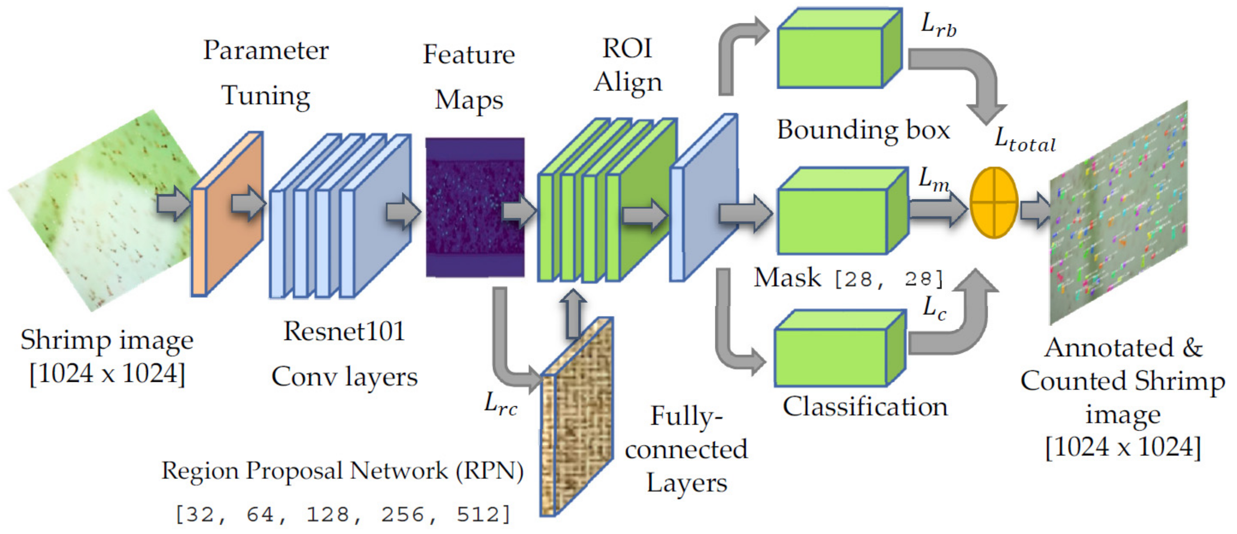
3. Mask R-CNN
4. Experimental Results and Analysis
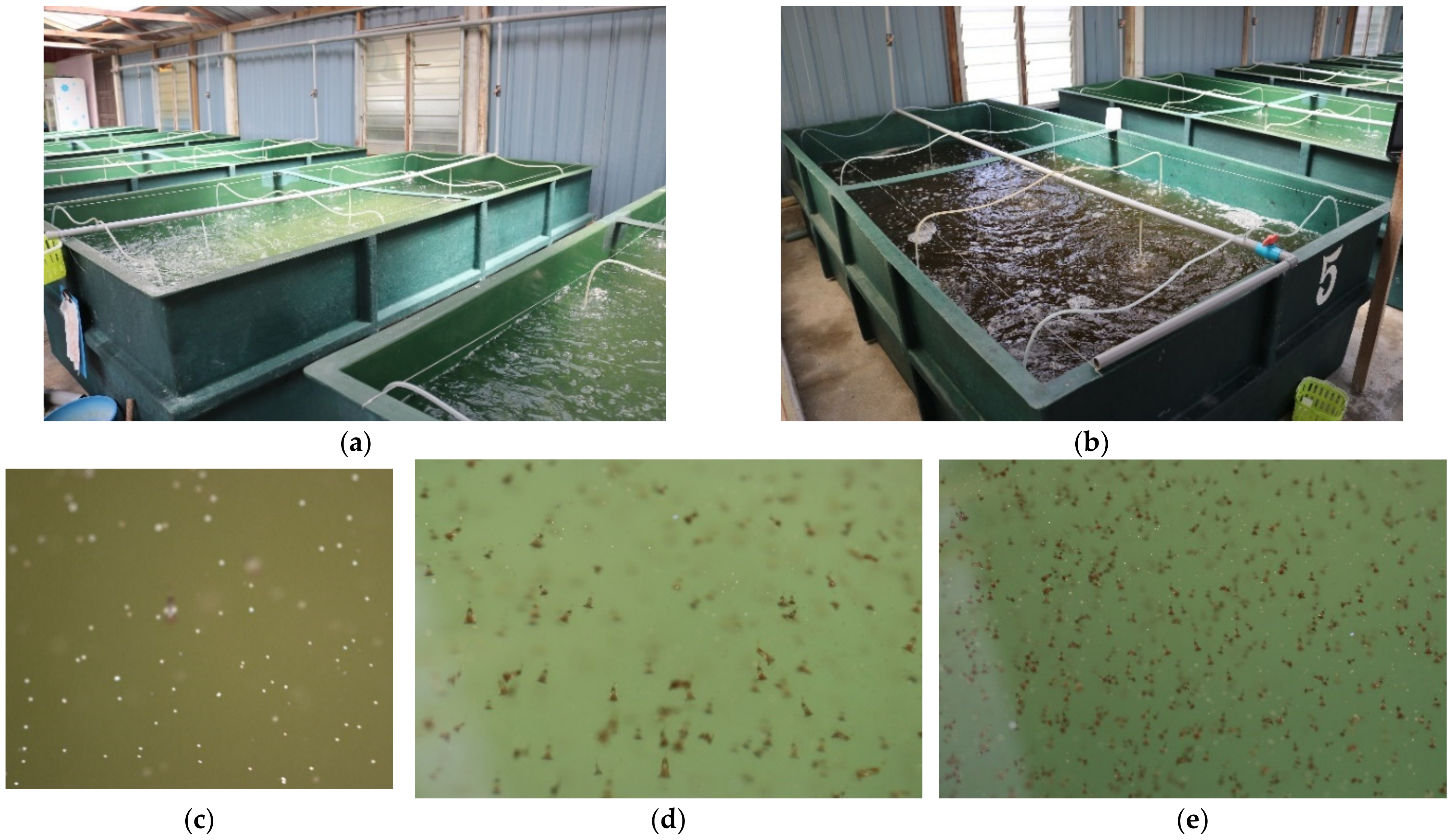
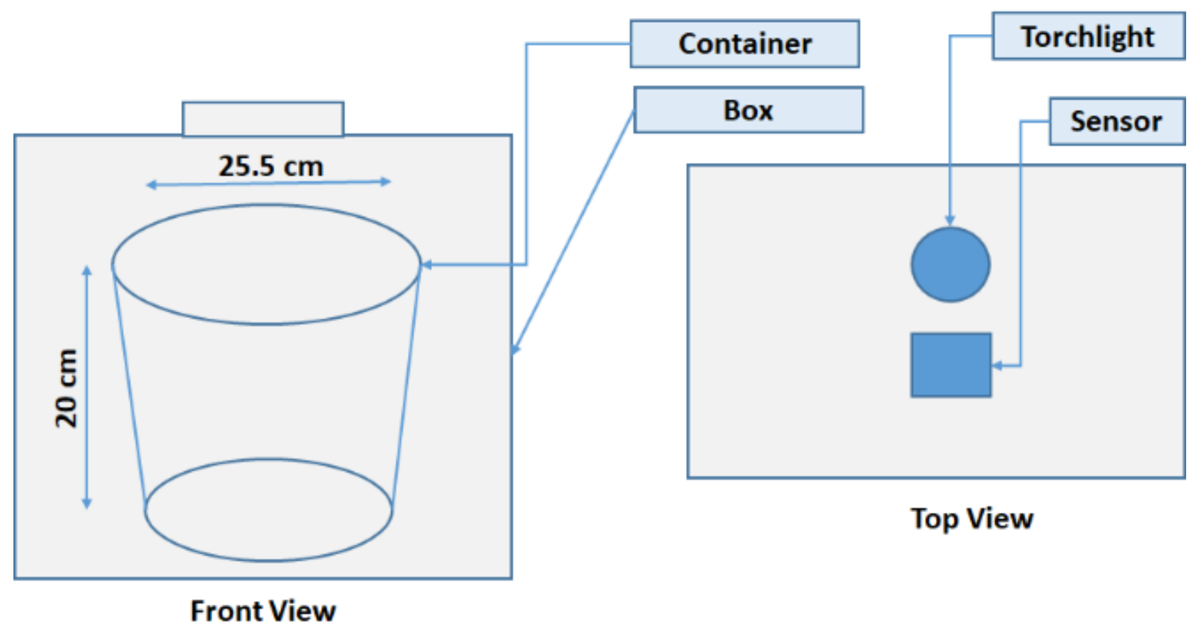
4.1. Building a Dataset
4.2. Training the Model
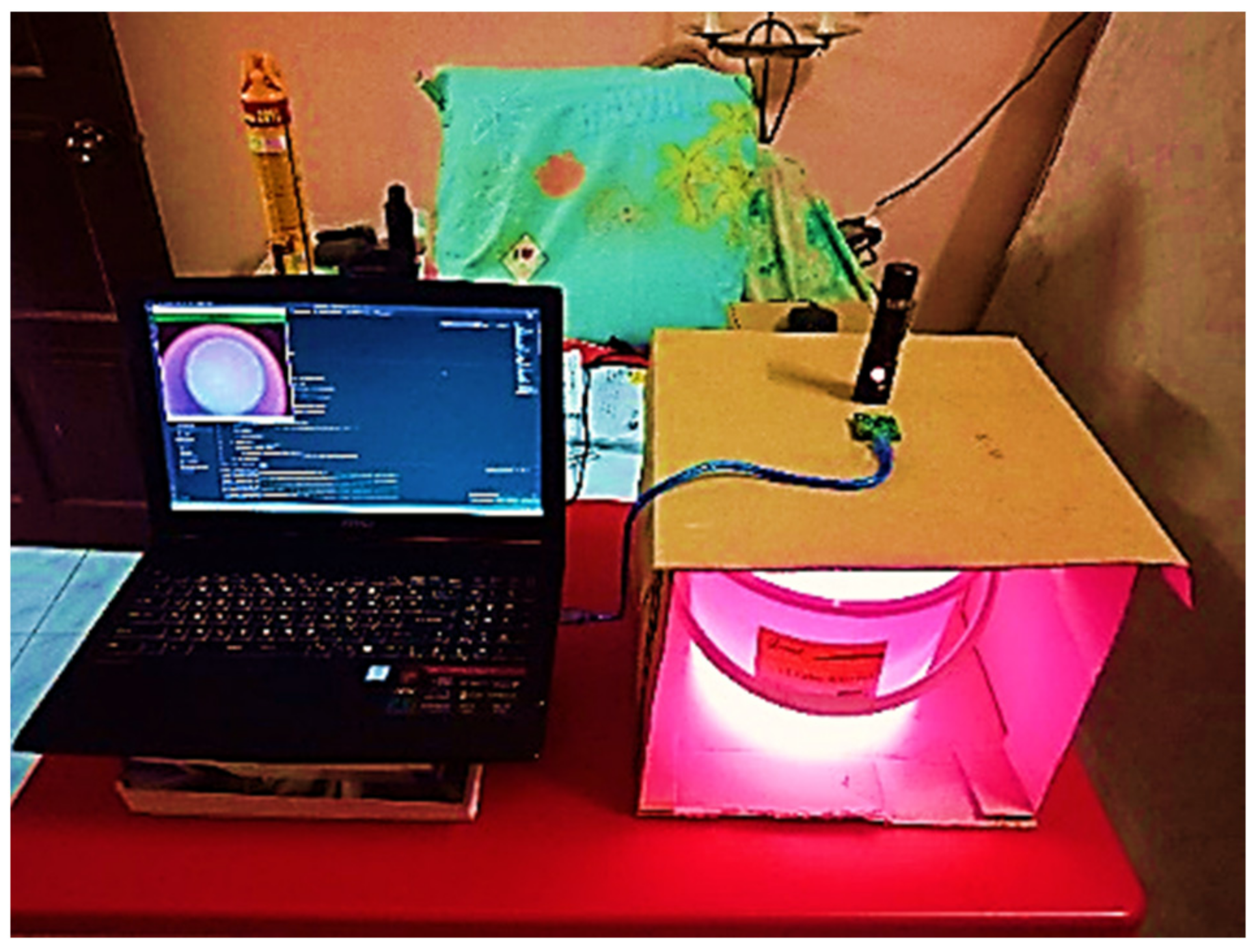
4.3. Experimental Environment
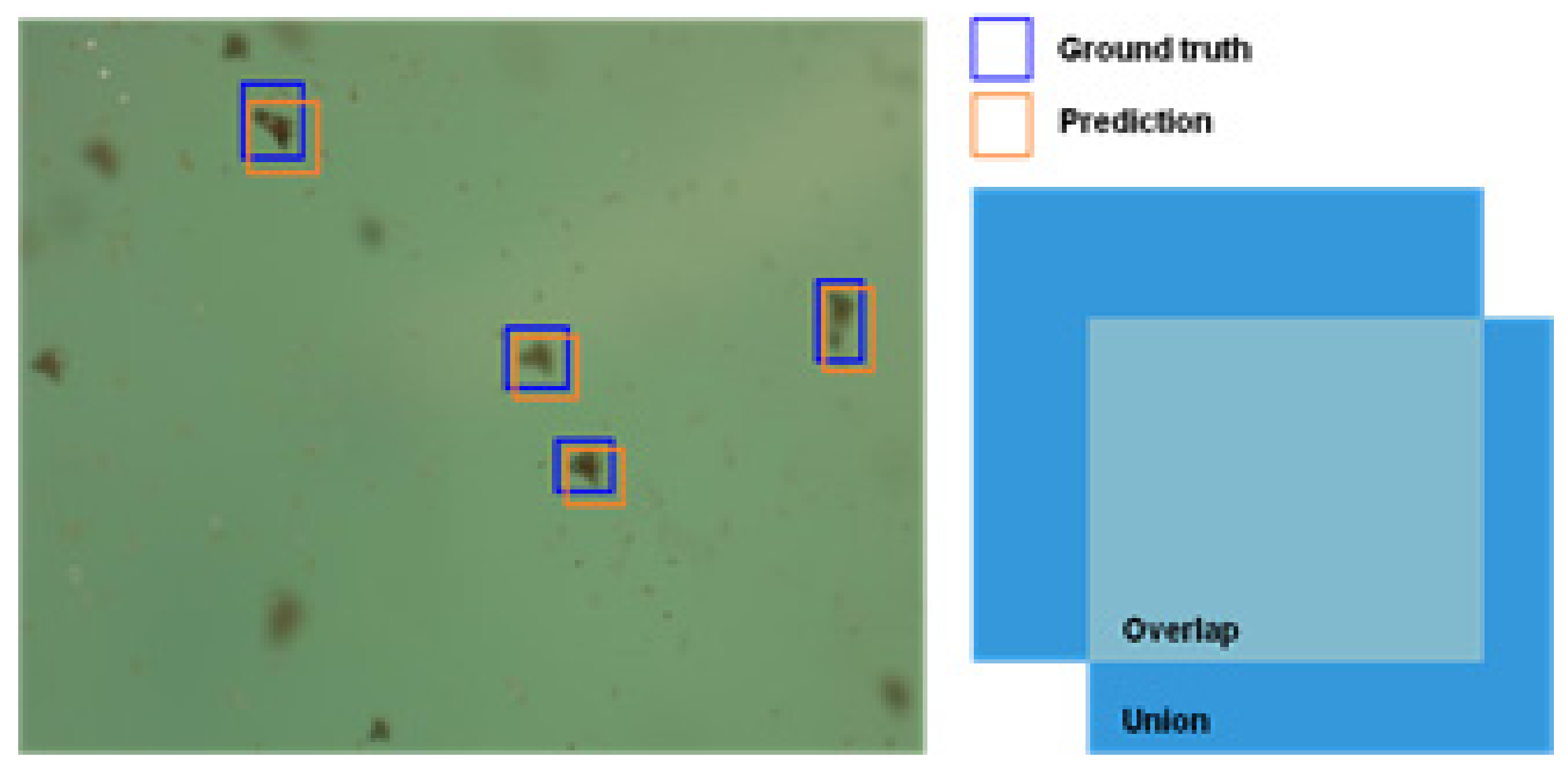
4.4. Evaluation Index
4.5. Experimental Results and Analysis
- i
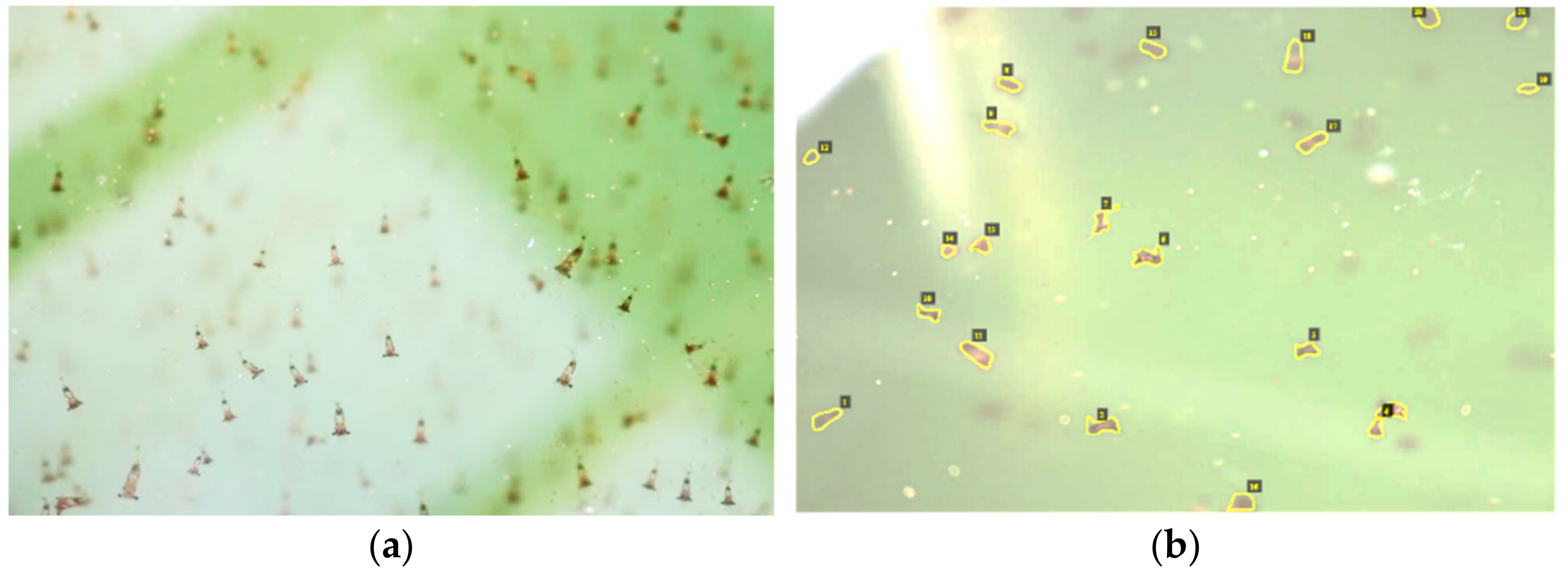
- The shrimp images were recorded from the top view with the assumption of equal size due to similar shrimp age kept in the container.
- ii
- It can automatically estimate the number of shrimps using computer vision and deep learning.
- iii
- Default Mask R-CNN can be manipulated to effectively segment and count tiny shrimps or objects.
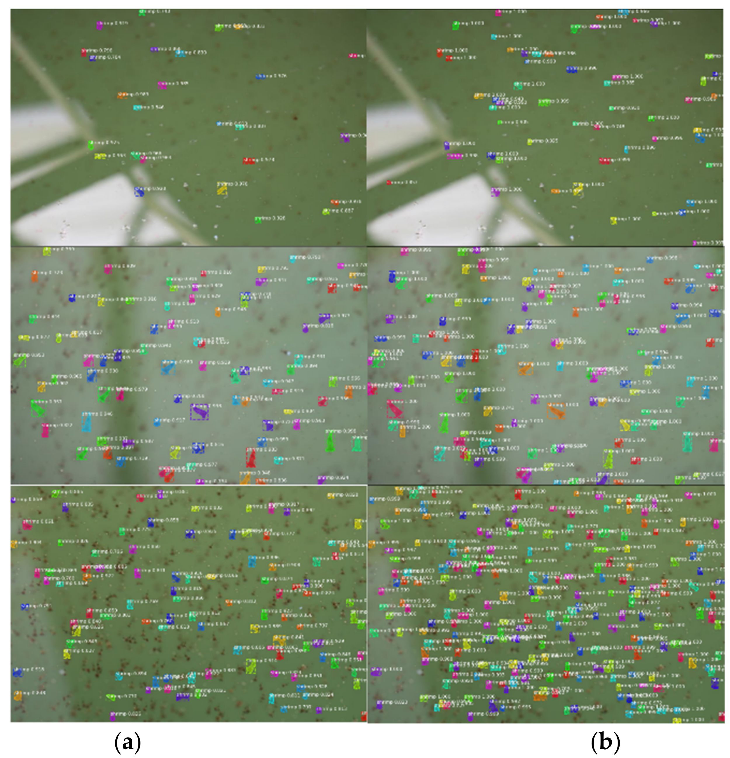
- iv
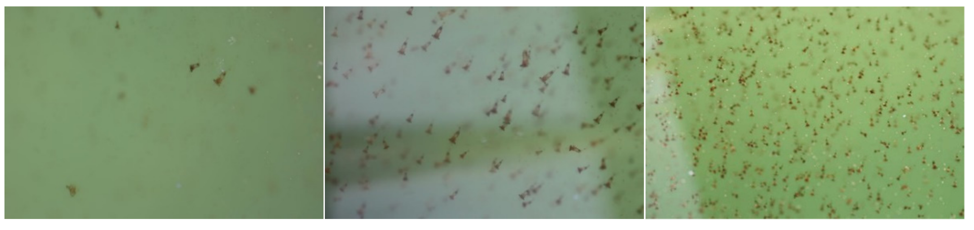
- The shrimp counting accuracy depreciates as the shrimp density increases or intensifies.
- v
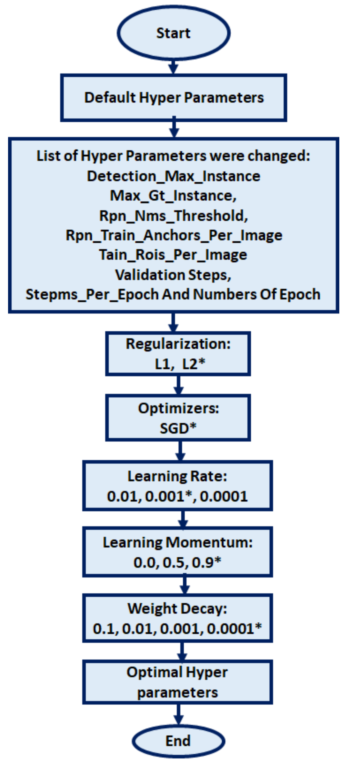
- The shrimp estimation efficacy has a linear proportion when the hyperparameters such as maximum detection instance, learning rate, maximum ground truth instance, RPN threshold value, RPN train anchors per image, the number of steps per epoch, train region of interest per image, validation steps, and weight decay are increasing.
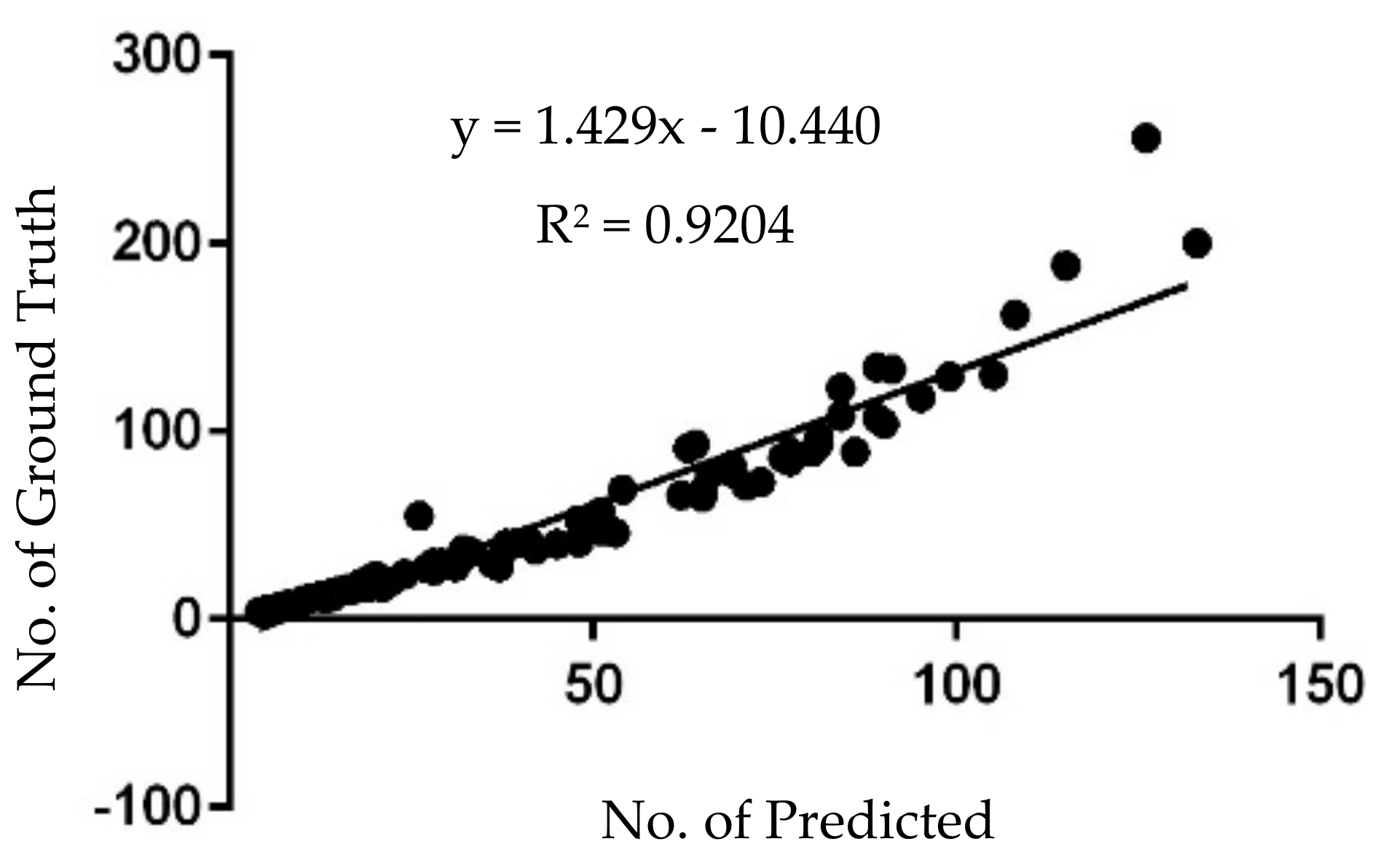
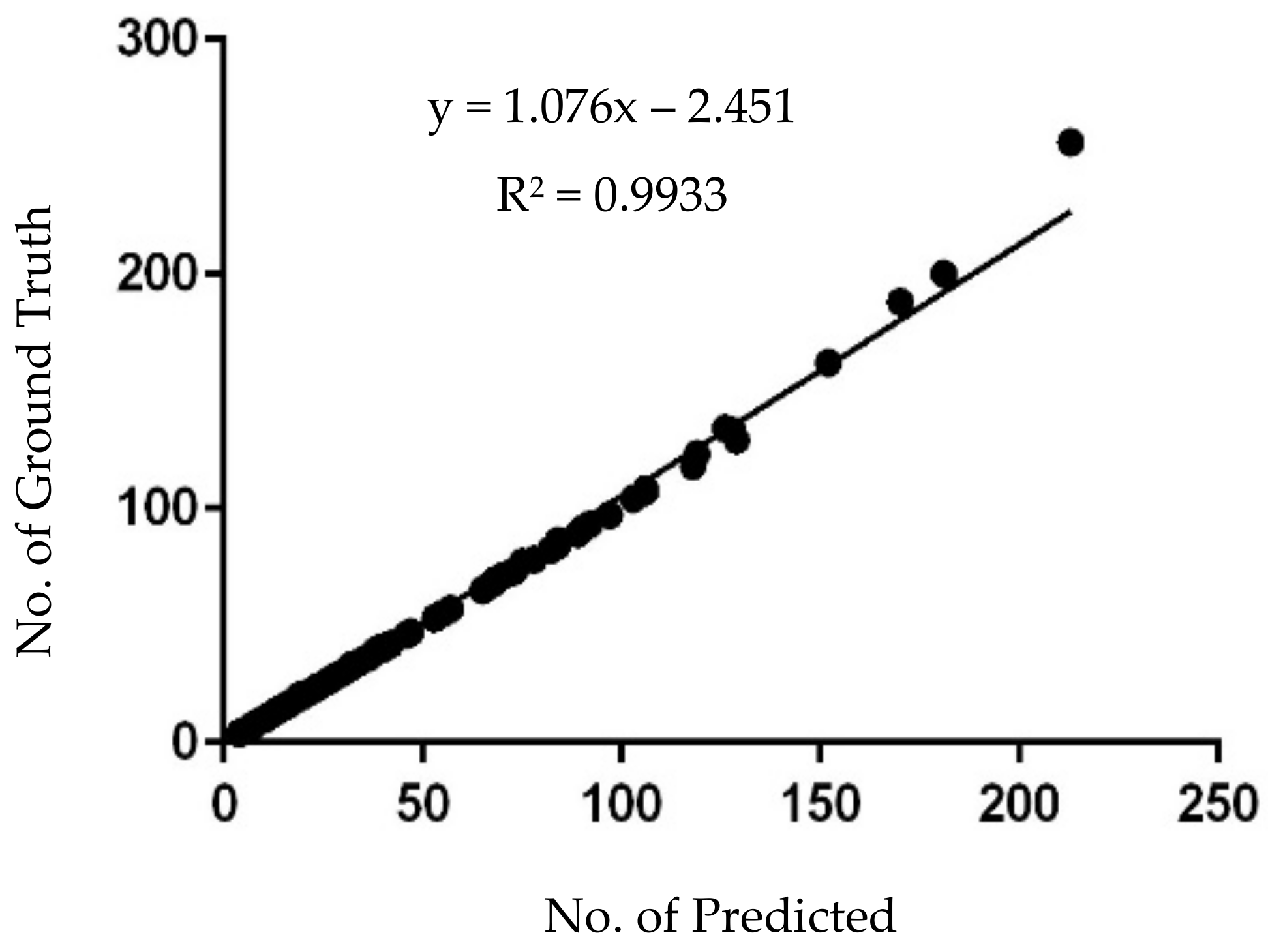
- vi
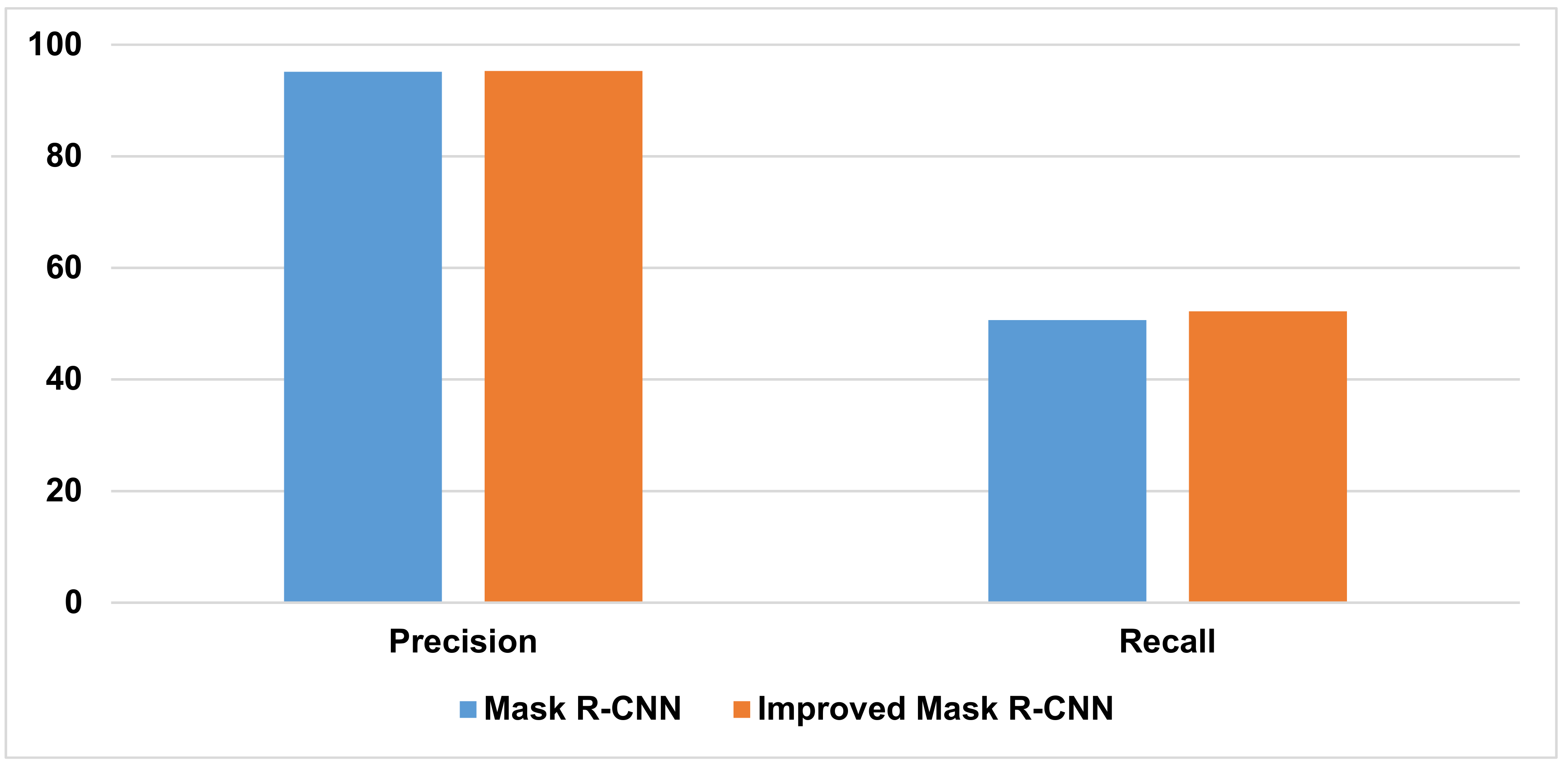
- The linear regression shows that increases with better precision after performing hyperparameter manipulation over the default Mask R-CNN.
- vii
- This application can reduce shrimp death risk compared to practicing manual counting.
5. Conclusions
Author Contributions
Funding
Data Availability Statement
Acknowledgments
Conflicts of Interest
Appendix A
| BACKBONE | resnet101 |
| BACKBONE_STRIDES | [4, 8, 16, 32, 64] |
| BATCH_SIZE | 1 |
| BBOX_STD_DEV | [0.1 0.1 0.2 0.2] |
| COMPUTE_BACKBONE_SHAPE | None |
| DETECTION_MAX_INSTANCES | 400 |
| DETECTION_MIN_CONFIDENCE | 0.7 |
| DETECTION_NMS_THRESHOLD | 0.3 |
| FPN_CLASSIF_FC_LAYERS_SIZE | 1024 |
| GPU_COUNT | 1 |
| GRADIENT_CLIP_NORM | 5.0 |
| IMAGES_PER_GPU | 1 |
| IMAGE_CHANNEL_COUNT | 3 |
| IMAGE_MAX_DIM | 1024 |
| IMAGE_META_SIZE | 14 |
| IMAGE_MIN_DIM | 800 |
| IMAGE_MIN_SCALE | 0 |
| IMAGE_RESIZE_MODE | square |
| IMAGE_SHAPE | [1024 1024 3] |
| LEARNING_MOMENTUM | 0.9 |
| LEARNING_RATE | 0.01 |
| LOSS_WEIGHTS | {'rpn_class_loss': 1.0, 'rpn_bbox_loss': 1.0, 'mrcnn_class_loss': 1.0, 'mrcnn_bbox_loss': 1.0, 'mrcnn_mask_loss': 1.0} |
| MASK_POOL_SIZE | 14 |
| MASK_SHAPE | [28, 28] |
| MAX_GT_INSTANCES | 400 |
| MEAN_PIXEL | [123.7 116.8 103.9] |
| MINI_MASK_SHAPE | (56, 56) |
| NAME | shrimp |
| NUM_CLASSES | 2 |
| POOL_SIZE | 7 |
| POST_NMS_ROIS_INFERENCE | 1000 |
| POST_NMS_ROIS_TRAINING | 2000 |
| PRE_NMS_LIMIT | 6000 |
| ROI_POSITIVE_RATIO | 0.33 |
| RPN_ANCHOR_RATIOS | [0.5, 1, 2] |
| RPN_ANCHOR_SCALES | (32, 64, 128, 256, 512) |
| RPN_ANCHOR_STRIDE | 1 |
| RPN_BBOX_STD_DEV | [0.1 0.1 0.2 0.2] |
| RPN_NMS_THRESHOLD | 0.8 |
| RPN_TRAIN_ANCHORS_PER_IMAGE | 512 |
| STEPS_PER_EPOCH | 100 |
| TOP_DOWN_PYRAMID_SIZE | 256 |
| TRAIN_BN | False |
| TRAIN_ROIS_PER_IMAGE | 300 |
| USE_MINI_MASK | True |
| USE_RPN_ROIS | True |
| VALIDATION_STEPS | 200 |
| WEIGHT_DEC | 0.001 |
References
- Ghazvini, A.; Abdullah, S.N.H.S.; Ayob, M. A Recent Trend in Individual Counting Approach Using Deep Network. Int. J. Interact. Multimed. Artif. Intell. 2019, 5, 7–14. [Google Scholar] [CrossRef] [Green Version]
- Abdullah, S.N.H.S.; Zaini, A.S.; Yilmaz, B.; Abdullah, A.; Othman, N.S.M.; Kok, V.J. Contour Based Tracking for Driveway Entrance Counting System. Int. J. Integr. Eng. 2019, 11, 1–10. [Google Scholar] [CrossRef]
- Abu-Ain, T.A.K.; Abdullah, S.N.H.S.; Omar, K.; Abd Rahman, S.Z. Advanced Stroke Labeling Technique Based on Directions Features for Arabic Character Segmentation. Asia-Pac. J. Inf. Technol. Multimed. 2019, 8, 97–127. [Google Scholar] [CrossRef]
- Abdullah, S.N.H.S.; Abdullah, S.; Petrou, M.; Abdullah, S.; Fitriayanshah, A.; Razalan, M.H.A. A portable rice disease diagnosis tool based on bi-level color image thresholding. Appl. Eng. Agric. 2016, 32, 295–310. [Google Scholar] [CrossRef]
- Alomari, Y.M.; Abdullah, S.N.H.S.; Zin, R.R.M.; Omar, K. Iterative Randomized Irregular Circular Algorithm for Proliferation Rate Estimation in Brain Tumor Ki-67 Histology Images. Expert Syst. Appl. 2015, 48, 111–129. [Google Scholar] [CrossRef]
- Solahudin, M.; Slamet, W.; Dwi, A.S. Vaname (Litopenaeus vannamei) Shrimp Fry Counting Based on Image Processing Method. IOP Conf. Ser. Earth Environ. Sci. 2018, 147, 012014. [Google Scholar] [CrossRef]
- Kumar, G.; Bhatia, P.K. A Detailed Review of Feature Extraction in Image Processing Systems. In Proceedings of the 2014 Fourth International Conference on Advanced Computing & Communication Technologies, Rohtak, India, 8–9 February 2014. [Google Scholar] [CrossRef]
- Young, T.; Hazarika, D.; Poria, S.; Cambria, E. Recent Trends in Deep Learning Based Natural Language Processing. IEEE Comput. Intell. Mag. 2018, 13, 55–75. [Google Scholar] [CrossRef]
- Ruiz, L.A.; Recio, J.A.; Fernández-Sarría, A.; Hermosilla, T. A feature extraction software tool for agricultural object-based image analysis. Comput. Electron. Agric. 2011, 76, 284–296. [Google Scholar] [CrossRef] [Green Version]
- Khurana, U.; Turaga, D.; Samulowitz, H.; Parthasrathy, S. Cognito: Automated Feature Engineering for Supervised Learning. In Proceedings of the 2016 IEEE 16th International Conference on Data Mining Workshops (ICDMW), Barcelona, Spain, 12–15 December 2016; pp. 1304–1307. [Google Scholar] [CrossRef]
- Gai, J.; Tang, L.; Steward, B.L. Automated crop plant detection based on the fusion of color and depth images for robotic weed control. J. Field Robot. 2019, 37, 35–52. [Google Scholar] [CrossRef]
- Toh, Y.H.; Ng, T.M.; Liew, B.K. Automated Fish Counting Using Image Processing. In Proceedings of the 2009 International Conference on Computational Intelligence and Software Engineering, Wuhan, China, 11–13 December 2009. [Google Scholar] [CrossRef]
- Labuguen, R.T.; Volante, E.J.P.; Causo, A.; Bayot, R.; Peren, G.; Macaraig, R.M.; Libatique, N.J.C.; Tangonan, G.L. Automated fish fry counting and schooling behavior analysis using computer vision. In Proceedings of the 2012 IEEE 8th International Colloquium on Signal Processing and Its Applications (CSPA 2012), Malacca, Malaysia, 23–25 March 2012. [Google Scholar] [CrossRef]
- Fabic, J.N.; Turla, I.E.; Capacillo, J.A.; David, L.T.; Naval, P.C. Fish population estimation and species classification from underwater video sequences using blob counting and shape analysis. In Proceedings of the 2013 IEEE International Underwater Technology Symposium (UT 2013), Tokyo, Japan, 5–8 March 2013; pp. 1–6. [Google Scholar] [CrossRef]
- Subdurally, S.; Dya, D.; Pudaruth, S. Counting People Using Blobs and Contours. Int. J. Comput. Vis. Image Processing 2015, 3, 1–16. [Google Scholar] [CrossRef]
- Punn, M.; Bhalla, N. Classification of Wheat Grains Using Machine Algorithms. Int. J. Sci. Res. 2013, 2, 363–366. [Google Scholar]
- Nasirahmadi, A.; Sturm, B.; Olsson, A.C.; Jeppsson, K.H.; Müller, S.; Edwards, S.; Hensel, O. Automatic scoring of lateral and sternal lying posture in grouped pigs using image processing and Support Vector Machine. Comput. Electron. Agric. 2019, 156, 475–481. [Google Scholar] [CrossRef]
- Sethy, P.K.; Barpanda, N.K.; Rath, A.K.; Behera, S.K. Deep feature-based rice leaf disease identification using support vector machine. Comput. Electron. Agric. 2020, 175, 105527. Available online: https://www.sciencedirect.com/science/article/abs/pii/S0168169919326997 (accessed on 29 November 2021). [CrossRef]
- Rahnemoonfar, M.; Sheppard, C. Deep Count: Fruit Counting Based on Deep Simulated Learning. Sensors 2017, 17, 905. [Google Scholar] [CrossRef] [PubMed] [Green Version]
- Li, W.; Chen, P.; Wang, B.; Xie, C. Automatic Localization and Count of Agricultural Crop Pests Based on an Improved Deep Learning Pipeline. Sci. Rep. 2019, 9, 7024. [Google Scholar] [CrossRef] [PubMed]
- Wang, Z.; Walsh, K.; Koirala, A. Mango Fruit Load Estimation Using a Video Based MangoYOLO—Kalman Filter—Hungarian Algorithm Method. Sensors 2019, 19, 2742. [Google Scholar] [CrossRef] [PubMed] [Green Version]
- Liu, X.; Jia, Z.; Hou, X.; Fu, M.; Ma, L.; Sun, Q. Real-time Marine Animal Images Classification by Embedded System Based on Mobilenet and Transfer Learning. In Proceedings of the OCEANS 2019—Marseille, Marseille, France, 17–20 June 2019; pp. 1–5. [Google Scholar] [CrossRef]
- Merencilla, N.E.; Alon, A.S.; Fernando, G.J.O.; Cepe, E.M.; Malunao, D.C. Shark-EYE: A Deep Inference Convolutional Neural Network of Shark Detection for Underwater Diving Surveillance. In Proceedings of the 2021 International Conference on Computational Intelligence and Knowledge Economy (ICCIKE), Dubai, United Arab Emirates, 17–18 March 2021; pp. 384–388. [Google Scholar] [CrossRef]
- Li, L.; Dong, B.; Rigall, E.; Zhou, T.; Dong, J.; Chen, G. Marine Animal Segmentation. IEEE Trans. Circuits Syst. Video Technol. 2021. [Google Scholar] [CrossRef]
- He, K.; Gkioxari, G.; Dollár, P.; Girshick, R. Mask R-CNN. In Proceedings of the 2017 IEEE International Conference on Computer Vision (ICCV), Venice, Italy, 22–29 October 2017; pp. 2980–2988. [Google Scholar] [CrossRef]
- Ren, S.; He, K.; Girshick, R.; Sun, J. Faster R-CNN: Towards Real-Time Object Detection with Region Proposal Networks. IEEE Trans. Pattern Anal. Mach. Intell. 2016, 39, 1137–1149. [Google Scholar] [CrossRef] [Green Version]
- Boom, B.J.; He, J.; Palazzo, S.; Huang, P.X.; Beyan, C.; Chou, H.M.; Lin, F.P.; Spampinato, C.; Fisher, R.B. A research tool for long-term and continuous analysis of fish assemblage in coral-reefs using underwater camera footage. Ecol. Inform. 2014, 23, 83–97. [Google Scholar] [CrossRef] [Green Version]
- Spampinato, C.; Chen-Burger, Y.H.; Nadarajan, G.; Fisher, R.B. Detecting, Tracking and Counting Fish in Low Quality Unconstrained Underwater Videos. VISAPP 2008, 2008, 1–6. [Google Scholar]
- Patel, H.; Singh Rajput, D.; Thippa Reddy, G.; Iwendi, C.; Kashif Bashir, A.; Jo, O. A review on classification of imbalanced data for wireless sensor networks. Int. J. Distrib. Sens. Netw. 2020, 16, 4. [Google Scholar] [CrossRef]
- Iwendi, C.; Maddikunta, P.K.R.; Gadekallu, T.R.; Lakshmanna, K.; Bashir, A.K.; Piran, M.J. A metaheuristic optimization approach for energy efficiency in the IoT networks. Softw. Pract. Exp. 2021, 51, 2558–2571. [Google Scholar] [CrossRef]
- Wang, S.; Qureshi, M.A.; Miralles-Pechuaán, L.; Huynh-The, T.; Gadekallu, T.R.; Liyanage, M. Explainable AI for B5G/6G: Technical Aspects, Use Cases, and Research Challenges. arXiv 2021, arXiv:2112.04698. [Google Scholar]


| Citation and Year | Key Features of Designed Algorithms/Models (Key Objectives and Performance Metrics) | Advantages (Achieved Performance) | Limitations (Based on the Application-Specific Standard Requirements) | |
|---|---|---|---|---|
| Non-Machine Learning-Based Algorithms | Alomari et al. [2] | Cell counting using dynamic initialization and number of iterations | Reduce false positive rate, resolve easy and medium-density object image | Unresolved high-density object image |
| Abdullah et al. [4] | Car counting using adaptive blob edge analysis | Resolve medium- and low-resolution images | Unsupported to vary low-contrast image type | |
| Jingyao et al. [11] | Color depth fusion algorithm using Kinect V2 Sensor | High true-positive crop segmentation rates | Low localization accuracy for flower-shaped vegetation | |
| Y.H. Toh et al. [12] | Count fish using blob and pixel size analysis methods | Accuracy escalates as the median reference area by averaging the median area of higher fish test cases | As the number of intersecting fish increases, accuracy drops | |
| R.T. Labuguen et al. [13] | Count fish fry using adaptive binarization and time frame average | High accuracy with intermediate density | Accuracy drops below 75% as the number of fry fish exceeds 700 | |
| J.N. Fabic et al. [14] | Color histogram, canny edge and Zernike shape analysis to identify fish species (Acanthuridae and Scaridae) on underwater video fish sequences | Able to estimate close to the ground truth value | Overcount of less than 10% due to background elimination | |
| Subdurally et al. [15] | Calculate headcount using blob and contour analysis | The acceptable head detection rate | Low-value completeness factor for the contour method, skin pixel may vary from dark to bright pixels, and the threshold value effects if the focal length changes continuously. | |
| Machine Learning-Based Algorithms | Meesha et al. [16] | Extract wheat grading into five classes using image thresholding, morphological features, support vector machine, and neural network | SVM outperforms NN with 86.8% and 94.5% accuracy rates | Morphological features are exhaustively relying on the pixel roundness ratio, volume, and area |
| Abozar et al. [17] | Pig calculation and monitoring using support vector machine | Outperforms when counting lateral and sternal lying posture of gathered pigs | Open-floor, lying close to the feeders or pen wall distracts calculation performance because of alike colors | |
| Deep Learning-Based Algorithms | Sethy et al. [18] | Classifies four types of rice leaf diseases | Extracts deep features from resnet50 and mobilenetv2, typical and small CNN models, respectively, and classify them using the SVM classification model | |
| Maryam et al. [19] | Tomato estimation using three parallel layers concatenated into one that improvised the Inception-ResNet-A module | The occurrence number of ripe and half-ripe fruits can easily accumulate | Ignore green fruit counting | |
| Weilu et al. [20] | Overcome overlapping detections for pest counting with the introduction of CNN with the Zeiler and Fergus (ZF) model and a region proposal network (RPN) with non-maximum suppression (NMS) | Multi-scale images can reduce the error losses and decrease false positives | ZF Net + RPN is comparable to ResNet-50 and ResNet-100 | |
| Zhenglin et al. [21] | Mango plant counting using Kalman filter, Hungarian algorithm, and YOLO | LED lighting and a camera have low implementation costs because they exclude differential global navigation satellite system | Disregards localization within the orchard or tree segmentation | |
| Liu et al. [22] | MobileNetV2 model based on convolutional neural network (CNN) and transfer learning | Able to classify seven marine animals using a robot camera | Classification accuracy varies according to the number of individual animals in each captured image | |
| Merencilla et al. [23] | Shark EYE used YOLOv3 algorithm for object detection, multiscale prediction, and logistic regression-based bounding box prediction | The system uses a large collection of great white sharks’ datasets underwater for training, as sharks are hard to differentiate from other shark-like animals in an underwater environment | It needs further to be refined for a wearable device equipped with a wide-angle camera | |
| Li et al. [24] | Segment marine animals involving conch, fish, and crab with a complex environment, MAS3K datasets | Introduce an enhanced cascade decoder network (ECDNet) with multiple interactive feature enhancement modules (IFEMs) and cascade decoder modules (CDMs) | The single decoder and the influence of the number of CDMs need to improvise for better performance | |
| Parameter | Default Mask R-CNN | Improved Mask R-CNN |
|---|---|---|
| Regularization | L2 | L1 |
| Maximum Detection instance | 100 | 400 |
| Learning rate | 0.001 | 0.01 |
| Maximum ground truth instance | 100 | 400 |
| Name | NONE | SHRIMP |
| RPN threshold value | 0.7 | 0.8 |
| RPN train anchors per image | 256 | 512 |
| Number of Steps per epoch | 50 | 100 |
| Train Region of Interest per image | 200 | 300 |
| Validation steps | 50 | 200 |
| Weight decay | 0.0001 | 0.001 |
| Attribute Name | Attribute Value |
|---|---|
| Tensorflow version | 1.3.0 |
| Keras Version | 2.0.8 |
| RAM | 8 GB |
| Processor | Intel (R) Core TM i7-7700HQ CPU @ 2.80GHz |
| Graphics | GeForce GTX 1050 |
| Operating system version | Windows 10 Pro, 64 bit |
| Symbol | Meaning |
|---|---|
| The number of images consisting of shrimp has been correctly localized | |
| The number of images unsuccessfully or partially localize the shrimp | |
| The number of images unsuccessfully localize the shrimp | |
| is the average accuracy average precision for a particular query | |
| A particular query | |
| Mean average precision by using all the point interpolation of precision and recall | |
| Number of images in the training dataset | |
| ∑ | Summation |
| Predicted number of shrimps | |
| Number of ground truths |
| Train | Test | |||
|---|---|---|---|---|
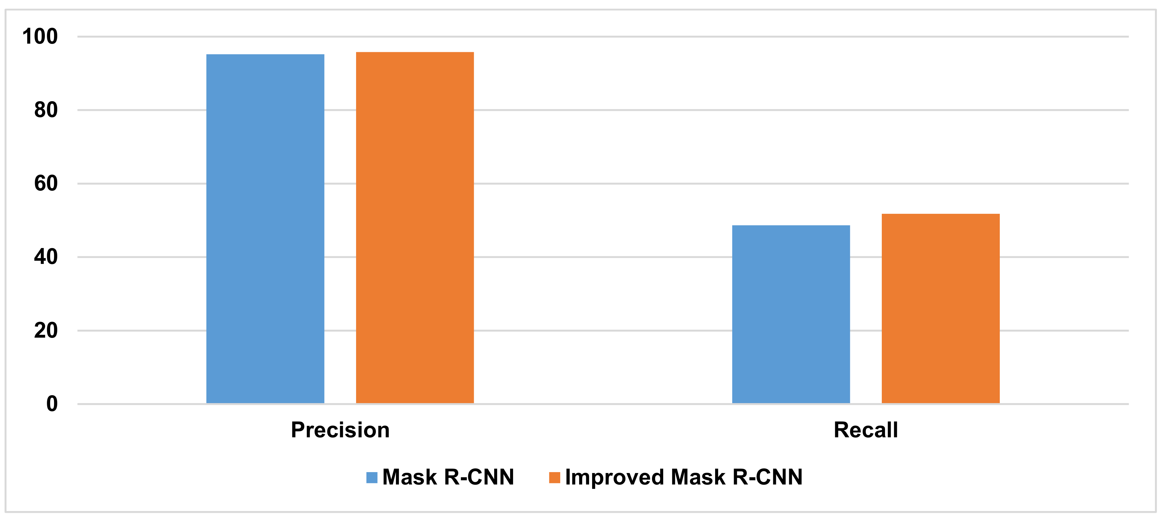
| Precision | Recall | Precision | Recall | |
| Mask R-CNN | 95.18% | 48.65% | 95.15% | 50.63% |
| Improved Mask R-CNN | 95.79% | 51.77% | 95.30% | 52.20% |
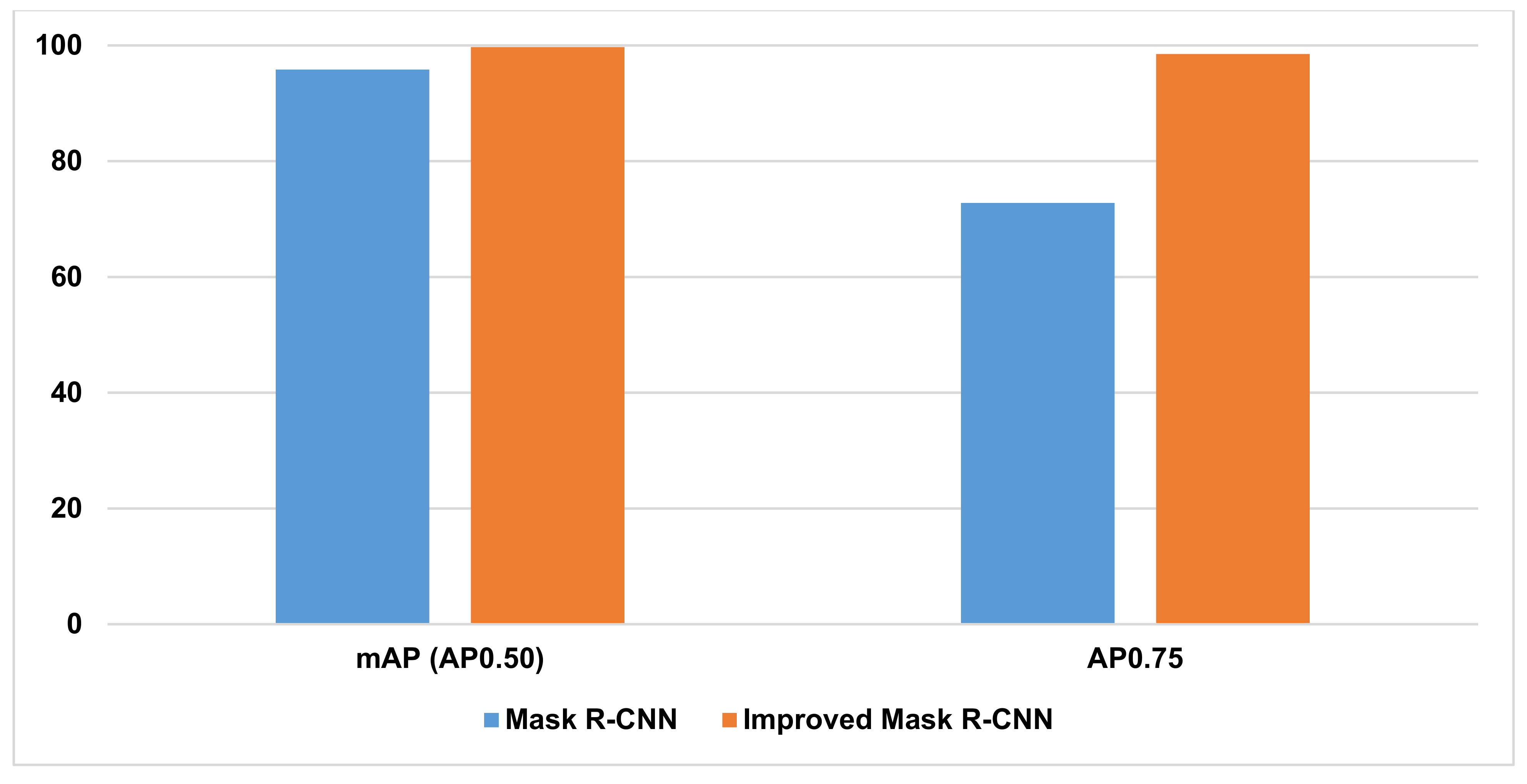
| Train | Test | |||
|---|---|---|---|---|
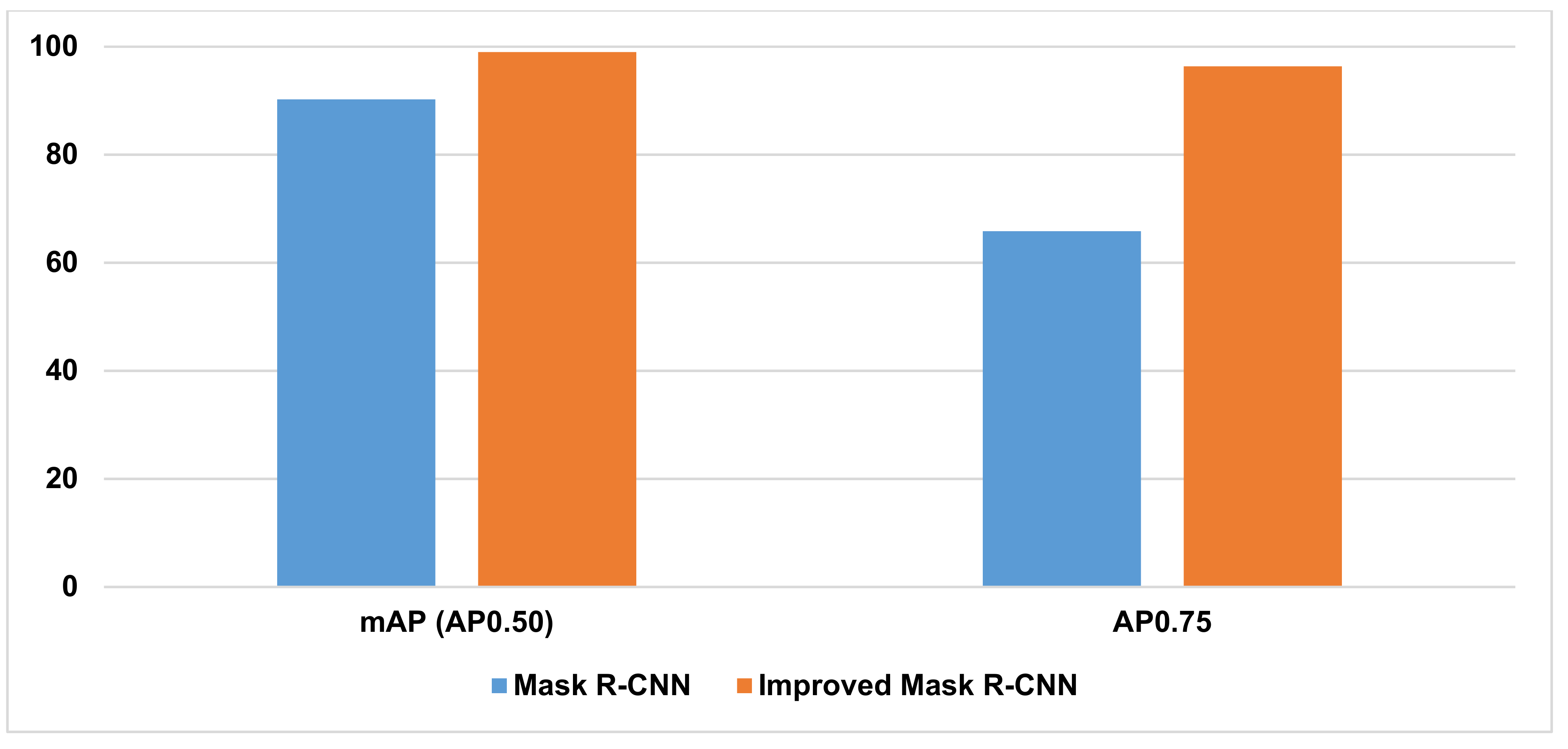
| mAP (AP0.50) | AP0.75 | mAP (AP0.50) | AP0.75 | |
| Mask R-CNN | 90.23% | 65.85% | 95.83% | 72.77% |
| Improved Mask R-CNN | 99.00% | 96.35% | 99.70% | 98.50% |
| Category | No. of Ground Truths | No. of Predicted Shrimps | Accuracy Rate | Error Rate |
|---|---|---|---|---|
| Less dense | 2682 | 2671 | 99.59% | 0.41% |
| Medium dense | 1715 | 1679 | 97.90% | 2.10% |
| Dense | 644 | 564 | 87.58% | 12.42% |
| Total | 5041 | 4914 | 97.48% | 2.52% |
Publisher’s Note: MDPI stays neutral with regard to jurisdictional claims in published maps and institutional affiliations. |
© 2022 by the authors. Licensee MDPI, Basel, Switzerland. This article is an open access article distributed under the terms and conditions of the Creative Commons Attribution (CC BY) license (https://creativecommons.org/licenses/by/4.0/).
Share and Cite
Hong Khai, T.; Abdullah, S.N.H.S.; Hasan, M.K.; Tarmizi, A. Underwater Fish Detection and Counting Using Mask Regional Convolutional Neural Network. Water 2022, 14, 222. https://doi.org/10.3390/w14020222
Hong Khai T, Abdullah SNHS, Hasan MK, Tarmizi A. Underwater Fish Detection and Counting Using Mask Regional Convolutional Neural Network. Water. 2022; 14(2):222. https://doi.org/10.3390/w14020222
Chicago/Turabian StyleHong Khai, Teh, Siti Norul Huda Sheikh Abdullah, Mohammad Kamrul Hasan, and Ahmad Tarmizi. 2022. "Underwater Fish Detection and Counting Using Mask Regional Convolutional Neural Network" Water 14, no. 2: 222. https://doi.org/10.3390/w14020222
APA StyleHong Khai, T., Abdullah, S. N. H. S., Hasan, M. K., & Tarmizi, A. (2022). Underwater Fish Detection and Counting Using Mask Regional Convolutional Neural Network. Water, 14(2), 222. https://doi.org/10.3390/w14020222