Use of Hyperspectral Reflectance and Water Quality Indices to Assess Groundwater Quality for Drinking in Arid Regions, Saudi Arabia

Abstract

Combining hydrogeochemical characterization and a hyperspectral reflectance measurement can provide knowledge for groundwater security under different conditions. In this study, comprehensive examinations of 173 groundwater samples were carried out in Makkah Al-Mukarramah Province, Saudi Arabia. Physicochemical parameters, water quality indices (WQIs), and spectral reflectance indices (SRIs) were combined to investigate water quality and controlling factors using multivariate modeling techniques, such as partial least-square regression (PLSR) and principal component regression (PCR). To measure water quality status, the drinking water quality index (DWQI), total dissolved solids (TDS), heavy metal index (HPI), contamination degree (C_d), and pollution index (PI) were calculated. Standard analytical methods were used to assess nineteen physicochemical parameters. The typical values of ions and metals were as follows: Na²⁺ > Ca²⁺ > Mg²⁺ > K⁺, Cl⁻ > SO₄²⁻ > HCO₃⁻ > NO₃⁻ > CO₃²⁻; and Cu > Fe > Al > Zn > Mn > Ni, respectively. The hydrogeochemical characteristics of the examined groundwater samples revealed that Ca-HCO₃, Na-Cl, mixed Ca-Mg-Cl-SO₄, and Na-Ca-HCO₃ were the main mechanisms governing groundwater chemistry and quality under the load of seawater intrusion, weathering, and water-rock interaction. According to the WQIs results, the DWQI values revealed that 2.5% of groundwater samples were categorized as excellent, 18.0% as good, 28.0% as poor, 21.5% as extremely poor, and 30.0% as unfit for drinking. The HPI and C_d values revealed that all groundwater samples had a low degree of contamination and better quality. Furthermore, the PI values showed that the groundwater resources were not affected by metals but were slightly affected by Mn in Wadi Fatimah due to rock–water interaction. Linear regression models demonstrated the significant relationships for the majority of SRIs paired with DWQI (R varied from −0.40 to 0. 75), and with TDS (R varied from 0.46 to 0.74) for the studied wadies. In general, the PLSR and PCR models provide better estimations for DWQI and TDS than the individual SRI. In conclusion, the grouping of WQIs, SRIs, PLSR, PCR, and GIS tools provides a clear image of groundwater suitability for drinking and its controlling elements.

1. Introduction

Groundwater is a fundamental and critical resource for humans all around the planet. Because of the importance of this resource, the world’s nations face a major challenge of water scarcity, especially in arid and semiarid regions [1,2]. Low precipitation and high evaporation rates in arid and semiarid regions increase water salinity, which increases the toxicity of some chemicals in groundwater [3]. According to recent studies, an estimated 2.1 billion people do not have access to adequate quality fresh water [4]. Water security that fulfils the quality specifications stipulated in relevant standards is currently the foundation for the operation of most communities [5].

Makkah Al-Mukarramah Province, located in southwest Saudi Arabia, has about 43 coastal wadies that are characterized by relatively heavy flashfloods and groundwater resources. It is a densely populated area due to its religious location, which leads to a sharp increase in water demand and affects the quality of its water. The groundwater in the Makkah Al-Mukarramah region is the major source of water resources, which have decreased significantly over the past few years. As the KSA Vision “2030” aims to maximize the utilization of Kingdom resources, such as water, and keep them from deteriorating in order to provide a decent life for its citizens, and with the ever-increasing population, the need for natural resources increases in order to secure the needs of the society. Therefore, periodic and seasonal monitoring of groundwater levels and quality has become extremely important for evaluating groundwater and overcoming the problem of depletion and degradation of groundwater in this region. The traditional methods for assessing groundwater quality from sample collection, conservation, and laboratory analysis have become very difficult and costly. Therefore, it was necessary to propose an alternative solution to the periodic chemical analysis of water depending on the hydrochemical models, spectral reflectance measurements, and remote sensing technology.

Water quality management, water pollution control, and environmental preservation must all be emphasized in order to safeguard living circumstances [6,7]. Understanding groundwater chemistry is a necessary prerequisite for mechanism analysis and quality evolution [8,9,10]. Natural processes such as dissolution, percolation, precipitation, and cation exchange, as well as anthropogenic activities, define the mechanism for groundwater chemistry [11,12,13].

In past investigations, standard water quality indices (WQIs) were used to assess groundwater quality [14,15]. Considering the numerous hydrochemical criteria, the WQIs technique is ineffective for determining groundwater quality [16]. Because of its more complete calculation, the methodology for evaluating groundwater quality using numerous hydrochemical parameters is seen to be a more robust approach [17,18,19,20]. Therefore, the WQIs have been extensively used for assessing groundwater quality. Furthermore, the geography information system (GIS) is useful in determining the spatial distribution of WQI values. Global research has been conducted in order to establish appropriate water quality assessment methodologies, including the single factor index approach based on water body objectives and needs [21,22].

The most frequent techniques for assessing water quality are the DWQI, HPI, C_d, and PI. As a result, it is vital to improve the method used to compute the weight, which might represent tacit information included in data [23]. The WQIs are derived from a large information set that includes multiple water quality metrics from diverse places. Many WQIs have been established to serve as markers for evaluating water quality in both drinking and agriculture usages [24,25,26,27]. The primary purpose of WQIs is to transform large amounts of complex information into numeric datasets, which helps to improve knowledge of water quality. The DWQI might be established as a dependable measure, defined as a number that indicates the integrated influence of several water quality elements. As a result, The DWQI is calculated by assessing the combined effect of man-made and environmental activity in the hydro-geometry characteristics of groundwater in the study area [28].

Remote sensing, in conjunction with geospatial approaches, plays an important role in measuring and mapping environmental contamination by facilitating spatial assessment. These strategies rely on non-spatial data being spatially represented in order to map the researched parameter throughout the entire region, including non-surveyed locations [29]. Moreover, spatial data have made tremendous advances in health and environmental appraisal research, assisting in the detection of pollutants and the concerning environmental elements [30]. The integration of remote sensing and GIS, as well as field observations and laboratory experiments, have generated exceptional environmental visualization of data with the help of spatial variation maps, which facilitate strategic planning [31]. Many studies commonly employ the visible and near-infrared ranges of the sun spectrum to extract accurate connections between SRIs and single water quality metrics (SWQM). Total suspended solids, turbidity, and chlorophyll-a were typically assessed utilizing remote sensing monitoring equipment [32,33]. However, defining a single water quality standard based on water quality usage is problematic.

There is particularly limited information available on the efficacy of spectral indices for predicting drinking and irrigation indices for water. There is just one study that discovered how to assess the drinking water quality index for water using known models based on spectral reflectance measurements to classify water quality level for drinking [34]. Consequently, the purpose of this research was to assess the robustness of recently created and published SRIs for calculating groundwater water-quality indices in three chosen wadies (Marawani, Fatimah, and Qanunah) in the Makkah region. As a consequence, freshly generated spectrum indices coming from the two wavelengths in the spectra will be assessed by building correlation matrices (contour maps) based on linear, quadratic, and exponential equations. Instead of formulating indices, whole spectra were used on an empirical basis to best fit the model to predict the trait of interest. Partial least square regression (PLSR) and principal component regression (PCR) models are typical methods that define an empirical rationale for a fit of the accuracy model to predict traits of interest [35]. Because the characteristics may be examined throughout a wide range of wavelengths from the spectral regions VIS and NIR or based on spectral indices SRIs, the PLSR and PCR are regression techniques that may be used to reduce the amount of collinear spectral factors generated [36,37].

Our research focuses on assessing groundwater quality in three different wadies utilizing physiochemical parameters, WQIs, and the accuracy of proximal remote sensing based on spectral bands. The objectives of this study were to: (i) identify geochemical types and their controlling factors based on physical and chemical metrics; (ii) assess the suitability of groundwater for drinking in relation to WQIs; (iii) assess the performance of newly and published SRIs for estimating the four WQIs of DWQI, TDS, HPI, and C_d; and (iv) evaluate the efficacy of PLSR and PCR models depending on investigated SRIs to predicting the four WQIs.

By concentrating on the most useful water quality criteria, this research offers tools for improved decision making concerning groundwater quality assessment in arid regions to guarantee successful management, aids in the identification of contamination sources, and offers a clearer picture for the redesign of sampling methods.

2. Materials and Methods

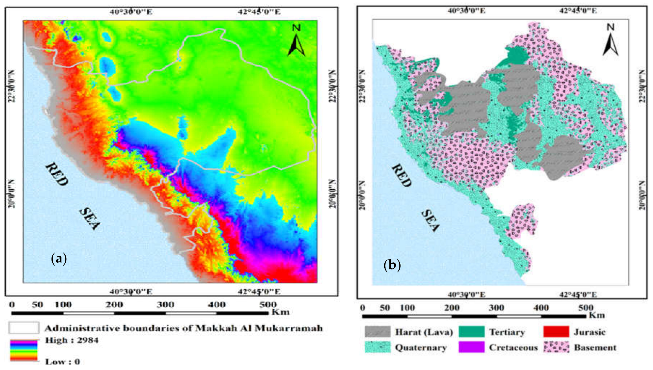
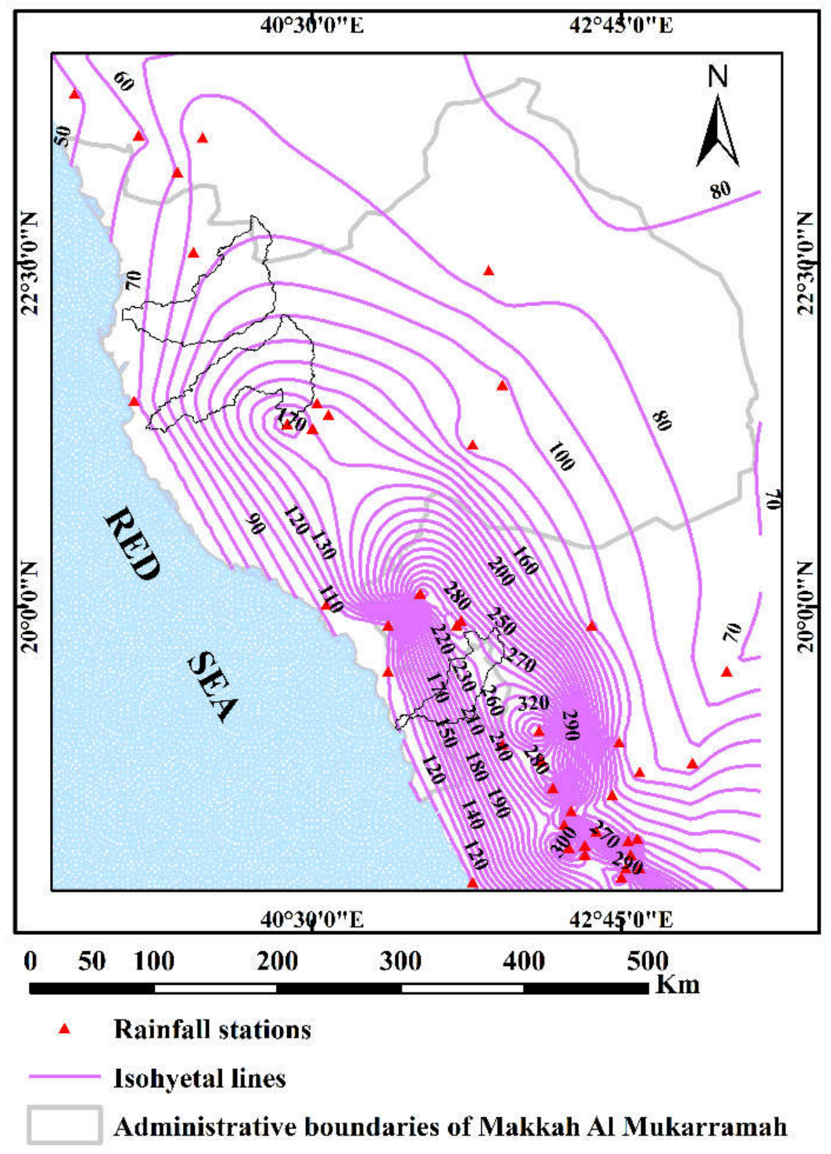
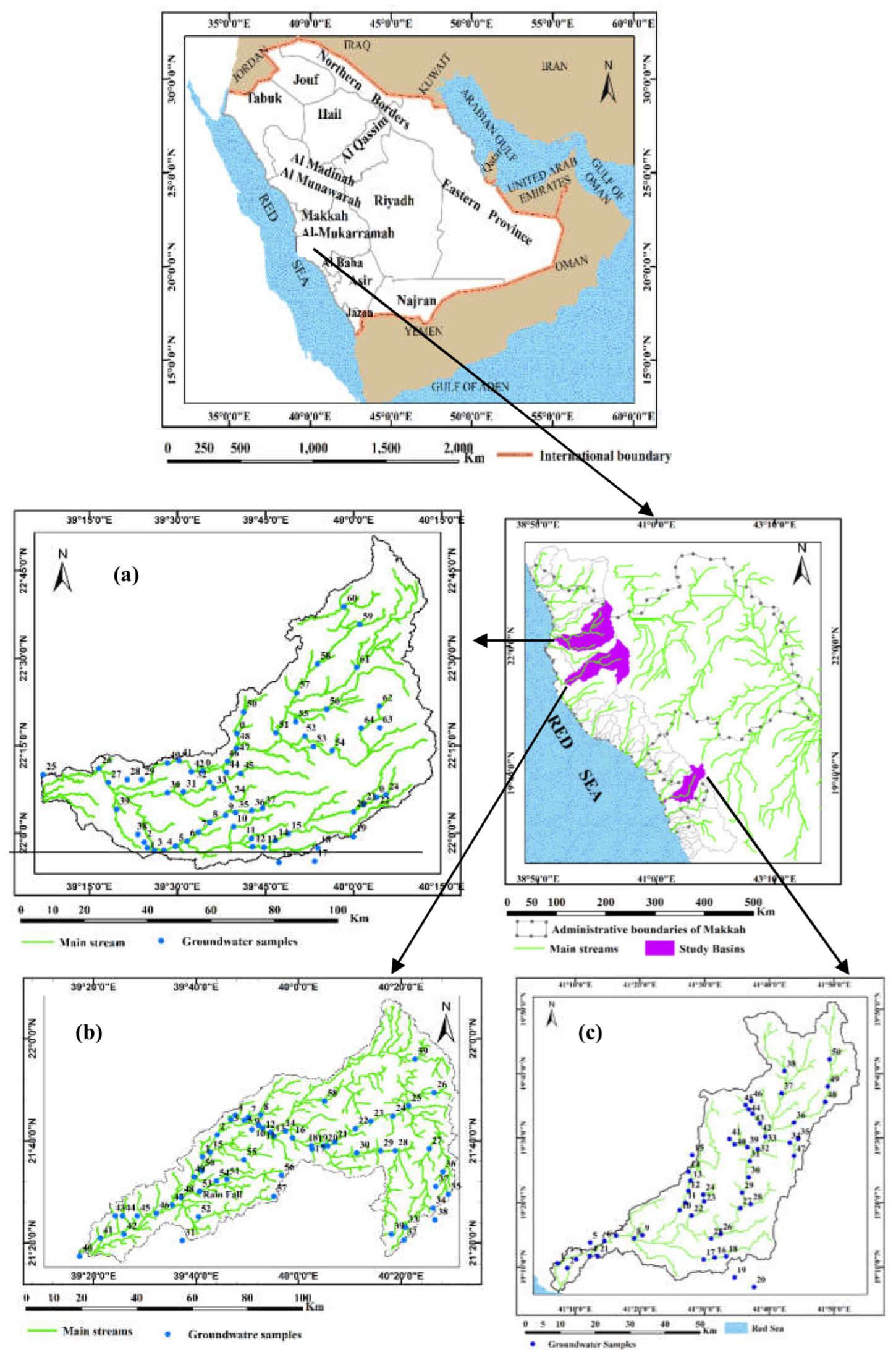
2.1. Study Wadies Description

The administrative borders of the Makkah province are bounded by the Red Sea in the west, Riyadh in the east, Al-Madinah Al-Munawarah in the north, and the Provinces of Al Bahaand Asir in the south, with a total area of 141,216 km² (Figure 1). This work was carried out under different condition in three representative wadies in Makkah Al-Mukarramah Province to evaluate the groundwater quality for drinking (Figure 1). Topographically, the Makkah region is characterized by a great diversity in altitude ranging from 0.0 m to 2984.0 m above mean sea level (amsl), as shown in Figure 2a [38]. Geologically, the lithological units that dominated in this area belong to the era that extends from the pre-Cambrian to the Quaternary (Figure 2b) [39]. The average annual precipitation distribution map in the Makkah region was constructed (Figure 3). Wadi Marawani, Wadi Fatimah, and Wadi Qanunah received an average rainfall of about 70–110 mm, 50–110 mm, and 100–400 mm, respectively, due to the presence of the upper mountainous region of the wadies [40].

Hydrogeological Description

The main water bearing formation in the selected wadies was the Quaternary aquifer, which is the primary source of groundwater for different uses. According to the information collected from the comprehensive survey of 173 groundwater wells, this aquifer was extended in coastal plains and wadi channels with a maximum thickness of about 118 m in Wadi Marawani, 60 m in Wadi Fatimah, and 74 m in Wad Qanunah. Lithologically, the Quaternary aquifer in the studied wadies in the Makkah region was formed mostly from alluvial deposits (gravel, sand, and silt) and the igneous metamorphic rocks form the bedrock of the aquifer, which were highly fractured and weather-cracked, making them an ideal host for groundwater preservation [40]. Therefore, the Quaternary aquifer in the study area is of an unconfined condition. As a result of the shallow depth of the groundwater and the porous and permeable deposits on top of the aquifer, human and agricultural activities could contribute to pollution in these wadies. The amount of rainfall distributed along these waterways is a major source of groundwater recharge. The majority of rainfall runoff infiltrates into highly permeable sediments that fill the wadi channels, where it recharges the shallow underlying Quaternary aquifer.

2.2. Groundwater Sampling

During 2021, groundwater samples were collected from the Quaternary aquifer along the three wadies. Sixty-four samples were taken from depths ranging between 1 and 30 m for Wadi Marawani, 59 samples from 1.2 to 50.1 m for Wadi Fatimah, and 50 samples between 0.8 and 21.7 m for Wadi Qanunah, through a surveying trip to convey the overall genuine conditions for assessing groundwater quality for drinking purposes. A portable GPS (MAGELLAN GPS 315, USA/United States of America) was used to determine the position of the water samples and identify the Universal Transverse Mercator coordinates system UTM of the research area (Figure 1).

2.3. Field Measurments and Laboratory Analysis

Portable conductivity multi-parameter equipment calibrated with standard solutions was used to determine T (°C), pH, EC, and TDS at the site (Hanna HI 9033, Germany). For chemical analysis, two groups of groundwater samples were obtained in 500 mL from each sampling location and filtered using 0.45 m Whatman filter paper. The samples were maintained at 4 °C until they were transported to the laboratory for physiochemical investigation. Using standard analytical procedures, twenty distinct physiochemical parameters were determined. The EDTA titrimetric approach was used to measure Mg²⁺ and Ca²⁺ concentrations, whereas a flame photometer was used to evaluate K⁺ and Na²⁺ concentrations (ELEX 6361, Hamburg, Germany). Titration with AgNO₃ was employed to measure Cl⁻ concentrations, whereas titrimetry was utilized to detect HCO₃⁻ and CO₃²⁻ concentrations. Sulfate (SO₄²⁻) and NO₃⁻ concentrations were determined using a spectrophotometer with UV spectrum (DR/2040 Loveland, USA). For analysis of trace element, samples were adjusted to a pH of 2 with conc. HNO₃ preservatives before being analyzed. Standard analytical protocols [41] were utilized to analyze metals such as Al, Cu, Fe, Mn, Ni, and Zn with an inductively coupled plasma mass spectrometer (ICP-MS, Waltham, USA/United States of America). Several quality assurance methods were employed throughout the evaluation of the water samples. The charge balance errors (CBE) were determined after the laboratory double-checked the experimental data using the formula below (Equation (1)).

$$\mathrm{CBE}=\frac{\sum \mathrm{Cations}-\sum \mathrm{Anions}}{\sum \mathrm{Cations}+\sum \mathrm{Anions}}\times 100$$

(1)

2.4. Measuring Spectral Reflectance

The spectral reflectance of the 173 collected groundwater samples from the three wadies was measured using a passive sensor (tec5, Oberursel, Germany). To study the link between the surface water spectrum in situ and the water quality indicators, a passive sensor with a viewing angle of 12° was utilized to measure the reflection of water. The water sample was placed in a glass jar, and the spectral reflectance of the water samples was measured at a distance of 0.30 m. A black sheet was used to cover the edges of the glass jar to avoid reflection from the backdrop and to collect all reflectance of water samples. The passive sensor has a spectral range from 302 nm to 1148 nm and a bandwidth of 2 nm [42]. The water reflection was obtained at a sunny period in a short time to eliminate variations in light radiation intensity, and each sample was a ten-scan average.

2.5. Selection of SRIs of Groundwater Samples of the Three Wadies

Fourteen SRIs, including five published indices and nine newly developed indices, were examined (

Table 1. Description of different SRIs used in this work.

SRIs	Formula	References
Published SRIs
Ratio between blue and red	Blue/Red	[43]
Ratio between green and red	Green/Red	[44]
Ratio between NIR and red	NIR/Red	[45]
Ratio between NIR and blue	NIR/Blue	[45]
Ratio between NIR and green	NIR/Green	[45]
New SRIs
RSI1122,454	R1122/R454	This work
RSI1122,470	R1122/R470
RSI1124,472	R1124/R472
RSI1122,480	R1122/R480
RSI1122,488	R1122/R488
RSI1122,510	R1122/R510
RSI1122,554	R1122/R554
RSI1124,570	R1122/R570
RSI1122,590	R1122/R590

). Contour maps were established to show determination coefficients (R²) between the DWQI, TDS, HPI, and C_d of water samples with ratio spectral indices (RSI). For example, the best RSI was determined by combining two separate wavelengths in the spectra ranging from 302 to 1148 nm for DWQI of three wadies: (a) Wadi Marawani, (b) Wadi Fatimah, and (c) Wadi Qanunah, as shown in Figure 4. The spectral reflectance contour maps of the spectrum region were constructed, which could be used to determine the effective spectral area with optimum wavelengths and to recognize the importance of SRIs. SRIs were calculated using thirteen wavelengths (454, 470, 472, 480, 488, 510, 480, 510, 554, 570, 590, 1122, and 1124 nm).

As indicated in Table 1, a ratio spectral index was calculated using this equation:

RSI = R₁/R₂

(2)

where R₁ and R₂ refer to the values of spectral reflectance at various wavelengths.

The linear fitting equation: Y = a + b RSI

(3)

2.6. Indexing Approach

The DWQI, HPI, C_d, and PI were calculated based on cited references [46,47,48,49] to detect the suitability of groundwater quality in the three selected wadies.

2.6.1. Drinking Water Quality Index (DWQI)

The DWQI were derived by the concentrations of thirteen determinants across the selected wadies (

Table 2. Arithmetic rating method for calculation of drinking water quality index (DWQI).

Physicochemical Parameters	Measured Sample	Si (mg/L) WHO (2011)	Unit Weight Wi	Sub Index (Qi)	${\mathbf{Q}}_{\mathbf{i}}\times {\mathbf{W}}_{\mathbf{i}}$
pH	7.70	8.5	0.4155	46.4162	19.2842
EC	3696.45	1500	0.0024	246.4297	0.5802
TDS	2214.00	500	0.0071	442.7992	3.1274
TH	1004.30	500	0.0071	200.8604	1.4187
K+	8.80	12	0.2943	73.3304	21.5802
Na2+	415.20	200	0.0177	207.5998	3.6656
Mg2+	89.34	50	0.0706	178.6869	12.6204
Ca2+	255.20	75	0.0471	340.2723	16.0220
Cl−	818.44	250	0.0141	327.3740	4.6244
SO42−	531.45	250	0.0141	212.5783	3.0028
HCO3−	186.25	120	0.0294	155.2062	4.5675
CO32−	2.39	350	0.0101	0.6837	0.0069
NO3−	46.83	50	0.0706	93.6599	6.6151
			∑ (Wi) = 1		${{\displaystyle \sum }}_{\mathrm{i}=1}^{\mathrm{n}}{\mathrm{Q}}_{\mathrm{i}}\times { \mathrm{W}}_{\mathrm{i}}$

). The results of all laboratory analyses for all groundwater wells obtained were examined for quality review. The physicochemical parameters were weighted depending on their relevance in the overall quality of water for water supply. According to Equation (4), the DWQI displays the overall water quality of each water component as a function of a range of water quality factors and their utilization in the ecosystem [50].

$$\mathrm{DWQI}={{\displaystyle \sum }}_{\mathrm{i}=1}^{\mathrm{n}}{\mathrm{W}}_{\mathrm{i}} \times (\frac{{\mathrm{C}}_{\mathrm{i}}}{{\mathrm{S}}_{\mathrm{i}}}\times 100)$$

(4)

where W_i indicates the weight unit of each parameter, and 13 physical and chemical parameters were used. The concentration (C_i) and standard (S_i) values for each water variable were derived using the formula below (Equation (5)):

$${\mathrm{W}}_{\mathrm{i}}=\frac{{\mathrm{w}}_{\mathrm{i}}}{\sum {\mathrm{w}}_{\mathrm{i}}}$$

(5)

Equation (6) computes w_i for each parameter using the accepted criteria [51]:

w_i = K/S_i

(6)

where K denotes the proportionality factor.

To calculate the DWQI, each groundwater variable (w_i) is weighted, and the relative weight is established (W_i). Therefore, the values of W_i were given to totally physicochemical parameters, and w_i was computed using Equation (7). Table 2 displayed the calculated values of the water parameters’ standards, weights (w_i), and arithmetic weights (W_i).

2.6.2. Water Pollution Indices (PIs)

Heavy Metal Pollution Index (HPI)

To determine total groundwater quality, a toxicity index (HPI) based on rating the mathematical weights of metals was utilized (

Table 3. The HPI, C_d, and PI are computed using an arithmetic rating approach.

Trace Element (mg/L)	Measured Sample	Si (mg/L) (WHO, 2011)	MACi	Unit Weight Wi	Sub Index Qi	${\mathbf{Q}}_{\mathbf{i}}\times {\mathbf{W}}_{\mathbf{i}}$
Al	0.003	0.2	200	0.072	1.500	0.108
Cu	0.08	2	2000	0.007	4.000	0.029
Fe	0.016	0.3	300	0.048	5.333	0.257
Mn	0.002	0.1	100	0.145	2.000	0.289
Ni	0.014	0.02	20	0.723	70.000	50.602
Zn	0.006	3	3000	0.005	0.200	0.001
				∑ (Wi) = 1		${{\displaystyle \sum }}_{\mathrm{i}=1}^{\mathrm{n}}{\mathrm{Q}}_{\mathrm{i}}\times { \mathrm{W}}_{\mathrm{i}}$

). The HPI values represent the cumulative effect of elements on overall groundwater quality [52] in comparison to the suggested standard recommendations (S_i) for each metal, namely, Al, Cu, Fe, Mn, Ni, and Zn. The HPI values were calculated using Equation (7):

$$\mathrm{HPI} =\frac{{{\displaystyle \sum }}_{\mathrm{i}=1}^{\mathrm{n}}{\mathrm{W}}_{\mathrm{i}}{\mathrm{Q}}_{\mathrm{i}}}{{{\displaystyle \sum }}_{\mathrm{i}-1}^{\mathrm{n}}{\mathrm{W}}_{\mathrm{i}}}$$

(7)

where W_i and Q_i are the corresponding unit weights and sub-indices for Al, Cu, Fe, Mn, Ni, and Zn, and n is the number of elements examined. There are three categories of HPI values: low heavy metal pollution (HPI > 100), heavy metal pollution with threshold risk (HPI = 100), and excessive heavy metal pollution (HPI > 100) [53].

Contamination Index (C_d)

The contaminated components of certain heavy metals that were above allowable levels were used to compute groundwater contamination degrees, which are expressed by C_d values [47,48] according to Equations (8) and (9):

$${\mathrm{C}}_{\mathrm{d}}={{\displaystyle \sum }}_{\mathrm{i}=1}^{\mathrm{n}}{\mathrm{C}}_{\mathrm{fi}}$$

(8)

$${\mathrm{C}}_{\mathrm{fi}}=\frac{{\mathrm{C}}_{\mathrm{Ai}}}{{\mathrm{C}}_{\mathrm{Ni}}}-1$$

(9)

where C_fi represents the contamination factor for each heavy metal, C_Ai represents the analytical value for each metal, C_Ni is the acceptable concentration of each element, and C_Ni is reserved as the maximum acceptable concentration.

Pollution Index (PI)

To assess the influence of heavy metal contamination for the groundwater quality, PI values were calculated. These demonstrate the particular contaminating impact of each heavy metal on groundwater quality and are categorized into five groups (

Table 4. Pollution levels as determined by PI according to Edet and Offong [48].

Class	PI Value	Effect
1	<1	No effect
2	1–2	Slightly affected
3	2–3	Moderately affected
4	3–5	Strongly affected
5	>5	Seriously affected

) based on Equation (10):

$$\mathrm{PI}=\frac{\sqrt{[(\frac{{\mathrm{C}}_{\mathrm{i}}}{{\mathrm{S}}_{\mathrm{i}}}{)}_{\max }^2+(\frac{{\mathrm{C}}_{\mathrm{i}}}{{\mathrm{S}}_{\mathrm{i}}}{)}_{\min }^2]}}{2}$$

(10)

where C_i denotes the metal content in water, and S_i indicates the metal level based on standards for each metal [54].

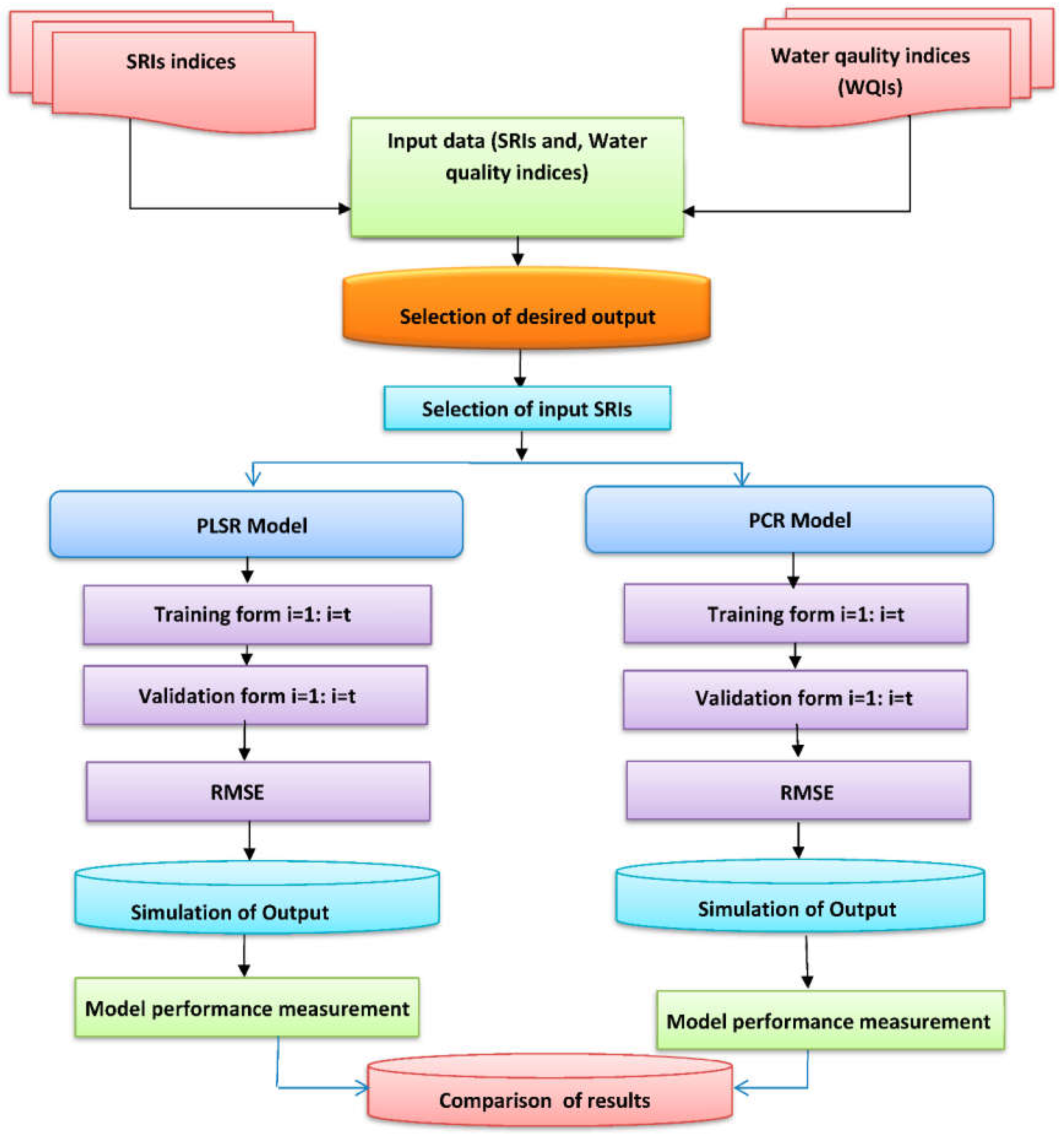
2.7. Partial Least-Square Regression (PLSR) and Principal Component Regression (PCR)

Both the PLSR and PCR models were utilized in this study to predict the DWQI, TDS, HPI, and C_d. Both models of the four WQIs were created using unscramble X software version 10.2. The two models (PLSR and PCR) included all selected SRIs in Table 1 as input datasets to forecast the four WQIs as output data for each wadi. The independent parameters were associated to the dependent parameter using leave-one-out cross-validation (LOOCV) for two models. The ideal number of latent variables (LVs) was selected based on the lowest value of RMSE to describe the calibration data without overfitting or underfitting (Figure 5). To strengthen the robustness of the results, the datasets were subjected to random 10-fold cross-validation.

Three metrics were employed to assess the two models’ effectiveness in predicting the four WQIs: R² coefficient, RMSE, and equation slope.

R² coefficient:

$${\mathrm{R}}^2=1-\frac{{{\displaystyle \sum }}_{\mathrm{i}=1}^{\mathrm{n}}{\left({\mathrm{WQIso}}_{\mathrm{i}}-{\mathrm{WQIs}}_{\mathrm{fi}}\right)}^2}{{{\displaystyle \sum }}_{\mathrm{i}=1}^{\mathrm{n}}{\left({\mathrm{PIso}}_{\mathrm{i}}\right)}^2}$$

(11)

RMSE:

$$\mathrm{RMSE}=\sqrt{\frac{{{\displaystyle \sum }}_{\mathrm{i}=1}^{\mathrm{n}}{\left({\mathrm{WQIso}}_{\mathrm{i}}-{\mathrm{WQIs}}_{\mathrm{fi}}\right)}^2}{\mathrm{n}}}$$

(12)

where $\mathrm{WQIs}$o_i is the measured value, n is the number of data points, and WQIs_fi is the predicted value.

2.8. Data Analysis and Graphical Approach

The descriptive statistics, including the minimum, maximum, and mean of the physicochemical parameters, WQIs, and SRIs, were calculated using SPSS 22 (SPSS Inc., Chicago, IL, USA). Hydrochemical facies generation models, such as the Piper and Gibbs diagrams, have been developed to establish groundwater types, geochemistry processes, and primary chemical control variables utilizing Geochemist’s Software package 12.0. In order to characterize the geochemical types of groundwater in the analyzed region, Piper’s trilinear diagram was used [55] to quantify the predominant cations and anions in meq/L of the collected groundwater samples. Gibbs diagram is widely used to establish a connection between groundwater composition and the aquifer matrix [56]. Gibbs diagram identifies the fundamental regulatory mechanisms that influence groundwater geochemistry by presenting TDS vs. (Na + K)/(Na + K + Ca) and Cl/(Cl + HCO₃). GIS version 10.0 was used to construct spatial variation maps for WQIs tested in this study. In addition, a combination of geo-statistical data processing and physicochemical characteristics was used to construct the WQI maps.

3. Results and Discussion

3.1. Physicochemical Parameters

Physicochemical metrics are significant criteria for assessing the geochemistry of groundwater and related signaling pathways, and so play a significant role in water quality management.

Table 5. Statistical analysis of the physical and chemical parameters of groundwater samples in the three selected wadies, Makkah Al-Mukarramah Province.

Physicochemical Parameters	Wadi Marawani (n = 64)			Wadi Fatimah (n = 59)			Wadi Qanunah (n = 50)
	Min.	Max.	Mean	Min.	Max.	Mean	Min.	Max.	Mean
T °C	24.00	31.00	27.30	30.00	32.00	30.66	23.00	30.00	26.04
pH	7.10	8.00	7.67	6.99	8.39	7.74	7.12	8.14	7.68
EC	658.00	28,700.00	4905.52	553.00	25,000.00	4217.27	429.00	4010.00	1534.26
TDS	346.00	18,171.00	2936.54	227.00	18,518.00	2572.27	208.00	2375.00	866.38
TH	67.18	7914.51	1298.81	44.17	6032.46	1189.46	136.31	1143.57	408.84
K+	0.79	28.10	8.12	0.99	79.03	13.87	0.60	13.57	3.69
Na+	38.00	5150.00	588.90	43.64	4602.76	441.93	24.10	641.40	161.32
Mg2−	9.30	710.00	129.67	4.12	575.28	90.56	9.00	133.40	36.28
Ca2+	11.60	2002.00	306.85	10.92	1995.81	327.26	34.50	415.00	104.08
Cl−	37.10	9666.00	1193.12	70.53	7271.04	926.22	14.70	901.50	211.65
SO42−	19.30	2840.00	609.62	30.01	5180.28	692.35	25.70	945.00	241.51
HCO3−	31.00	394.00	200.50	12.20	274.50	146.19	104.00	356.00	215.28
CO32−	N.D.	N.D.	N.D.	N.D.	24.00	7.02	N.D.	N.D.	N.D.
NO3−	2.20	290.70	53.99	0.01	475.44	57.28	0.78	160.80	25.34
Al	0.007	0.233	0.024	0.003	0.073	0.014	0.002	0.233	0.037
Cu	0.006	0.643	0.181	0.005	0.080	0.022	0.005	0.726	0.198
Fe	0.006	0.415	0.039	0.010	0.025	0.017	0.006	0.175	0.034
Mn	0.007	0.192	0.028	0.002	0.285	0.011	0.008	0.108	0.021
Ni	0.008	0.021	0.011	0.001	0.017	0.008	0.007	0.015	0.010
Zn	0.005	0.740	0.053	0.001	0.090	0.009	0.005	0.226	0.040

Note: Except for temperature (T °C), pH, and EC (µS/cm), all physical and chemical characteristics are provided in mg/L.

provides statistical summaries (min., max., mean) of the physicochemical properties of the groundwater locations studied in the three selected wadies.

The data analysis of physicochemical properties for groundwater samples from three wadies revealed that groundwater temperatures varied from 23.0 to 32.0 °C, with an average of around 28.08 °C based on well depths to the water surface. The pH readings varied from 6.99 to 8.39, with a mean of 7.69, indicating that the groundwater was mildly alkaline. The EC measurements varied from 429.0 to 28,700 µS/cm, with a mean of 3696.44 µS/cm. The TDS values ranged from 208.0 to 18518 mg/L, with a mean value of 2213.99 mg/L, which indicates brackish to saline groundwater, especially for Marawani and Fatimah basins, which indicated the possibility of seawater intrusion, especially in wells near the coast, and with the increase for discharging from those wells (mixing process). The relatively fresh water of Wadi Qanunah was due to the high annual rainfall amount along this wadi (100–400 mm), where infiltration rates are sufficient to fill the alluvial deposits within a short amount of time, and, consequently, at places of high permeability, and the surface water depressions appear directly connected to shallow unconfined aquifers [40]. The ionic content of K⁺, Na²⁺, Mg²⁺, Ca²⁺, Cl⁻, SO₄²⁻, HCO₃⁻, CO₃²⁻, and NO₃⁻ displayed mean values of 8.79, 415.19, 89.34, 415.19, 818.43, 531.44, 186.24, 2.39, and 46.82 mg/L, respectively (Table 5). Therefore, the average ion values displayed sequences of Na²⁺ > Ca²⁺ > Mg²⁺ > K⁺, and Cl⁻ > SO₄²⁻ > HCO₃⁻ > NO₃⁻ > CO₃²⁻, respectively. These values revealed that Na²⁺ was the dominant cation and Cl⁻ was the dominant anion for the collected water samples. The high concentration of NO₃⁻ in groundwater samples was mostly caused by nitrate fertilizer leaching from agricultural areas and domestic wastewater leakage from the nearby residential area [39]. The average concentrations of trace elements (Al, Cu, Fe, Mn, Ni, and Zn) across the selected wadies were 0.0239, 0.1316, 0.0300, 0.0204, 0.0095, and 0.0341 mg/L, respectively, which exhibited the following tendency: Cu > Fe > Al > Zn > Mn > Ni (Table 5). We know that trace elements in groundwater originate from a variety of sources, including weathering, soil leaching, and human activity. The quantities of trace elements in the analyzed groundwater samples showed low level of contamination by metals that were less than the specified permitted limits for drinking usages [50]. Accordingly, these elements were distributed uniformly, indicating that they were mainly derived from dissolution of silicate minerals in the aquifer matrix [39].

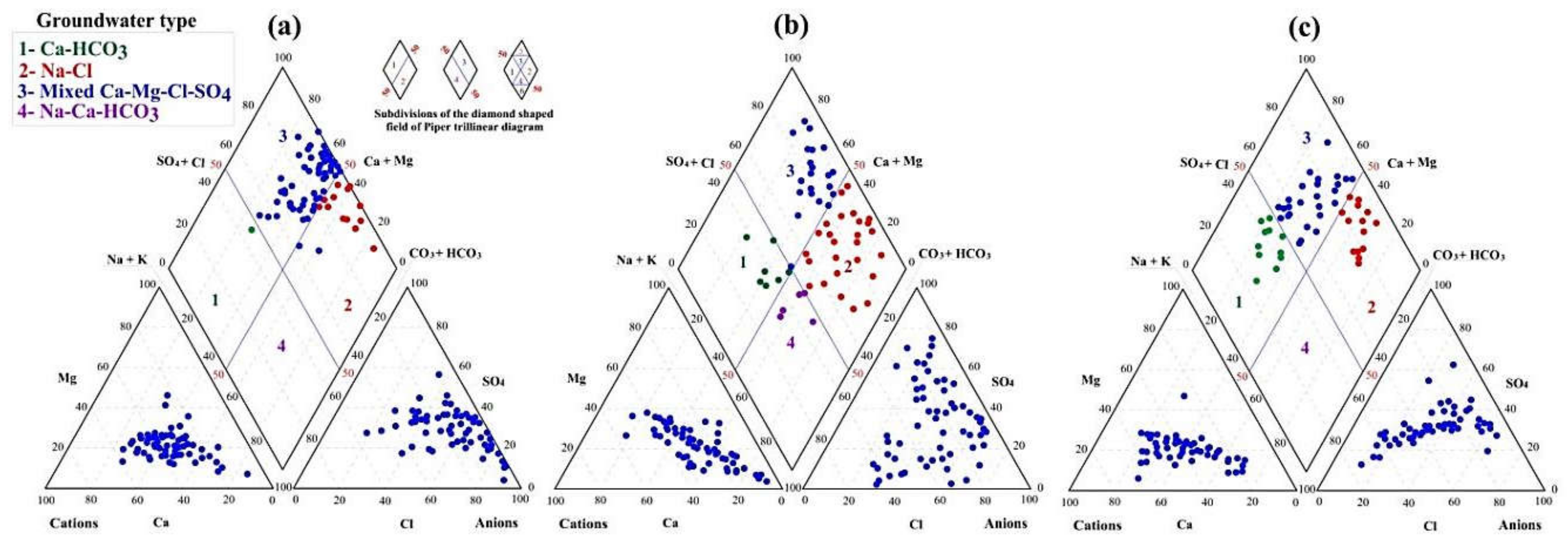
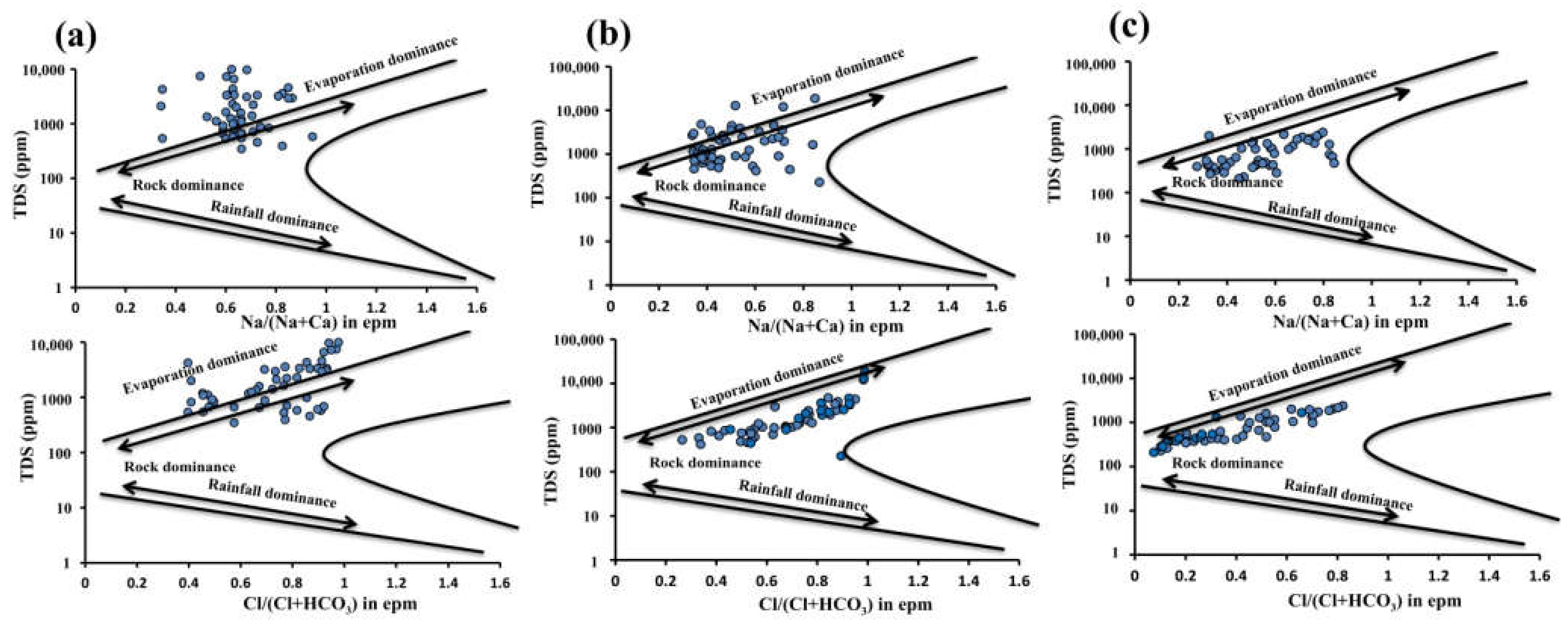
3.2. Geochemical Facies and Controlling Processes

Hydrogeochemical data analysis was conducted through illustrative methodologies, such as Piper and Gibbs diagrams, to better understand the different geochemical influences that control the groundwater quality in the studied wadies. According to the chemical characteristics of the groundwater samples analyzed, the hydrochemical facies were Ca-HCO₃, Na-Cl, mixed Ca-Mg-Cl-SO₄, and Na-Ca-HCO₃ (Figure 6). The weathering process and the aquifer matrix significantly alter the chemical composition of groundwater. A plot of chemical data on a Gibbs diagram (Figure 7) showed that the groundwater samples of the three wadies were distributed throughout the weathering and rock–water interactions fields [9].

3.3. Water Quality Indices

The statistical analysis and categorization of the various WQIs, including the DWQI, HPI, and C_d, employed in this study are shown in

Table 6. Classification of several water quality indices (WQIs).

WQIs	Min.	Max.	Mean	Range	Water Category	Number of Samples (%)
						Wadi Marawani (n = 64)	Wadi Fatimah (n = 59)	Wadi Qanunah (n = 50)
DWQI				0–25	Excellent	0 (0.0%)	1 (2.0%)	3 (6.0%)
				26–50	Good	7 (11.0%)	2 (3.0%)	22 (44.0%)
	22.69	545.53	97.11	51–75	Poor	24 (37.5%)	10 (17.0%)	15 (30.0%)
				76–100	Very poor	9 (14.0%)	19 (32.0%)	9 (18%)
				>100	Unsuitable	24 (37.5%)	27 (46.0%)	1 (2.0%)
HPI	5.07	77.41	38.74	<100	Low polluted	64 (100.0%)	59 (100.0%)	50 (100.0%)
				>100	High polluted	0 (0.0%)	0 (0.0%)	0 (0.0%)
Cd				<1	Low	64 (100.0%)	59 (100.0%)	50 (100.0%)
	−5.84	−2.90	−5.02	1–3	Medium	0 (0.0%)	0 (0.0%)	0 (0.0%)
				<3	High	0 (0.0%)	0 (0.0%)	0 (0.0%)

. Furthermore, spatial distribution maps for each index were utilized to present the quality of water in the researched basins (Table 6).

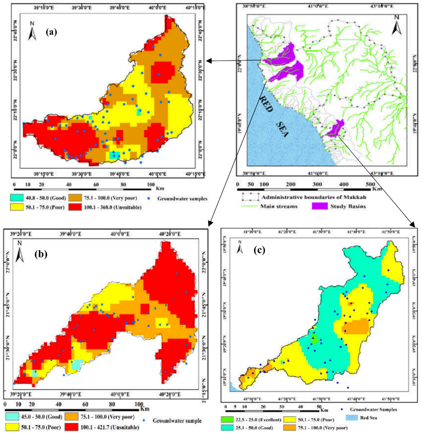
3.3.1. Drinking Water Quality Index (DWQI)

According to Equation (1), the WQIs models were applied to evaluate groundwater quality across three study locations, which were classified based on the purity of frequently stately water quality indices. The DWQI across the three wadies was created for assessing the appropriateness of groundwater for potable usages. Table 6 shows the calculated DWQI values in the acquired groundwater samples, which varied from 22.69 to 545.53, with an average of about 97.11. The DWQI categorization (Table 6) classified roughly 2.5% of groundwater as excellent, 18.0% as good, 28.0% as bad, 21.5% as extremely poor, and 30.0% as unfit for drinking due to the increase of Na²⁺ and Cl⁻ concentrations as a result of seawater intrusion, evaporation, and ion exchange processes. The DWQI distribution map (Figure 8) revealed that most of groundwater samples cannot be used for safe drinking due to the evaporation process, groundwater–rock interaction, reverse ion exchange processes, and seawater intrusion, as well as a low amount of rainfall, especially in the northern wadies of the Makkah region (Marawani and Fatimah). At the same time, in Wadi Qanunah in the south of Makkah, 50% of the samples ranged from excellent to good water for drinking use due to the floods following the rains, which have a positive impact on the recharge of groundwater in the area and its quality.

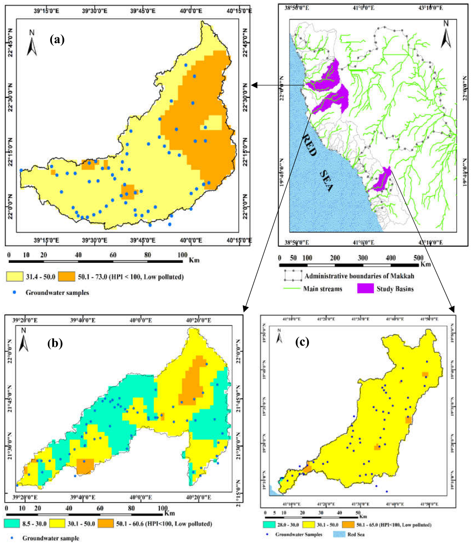
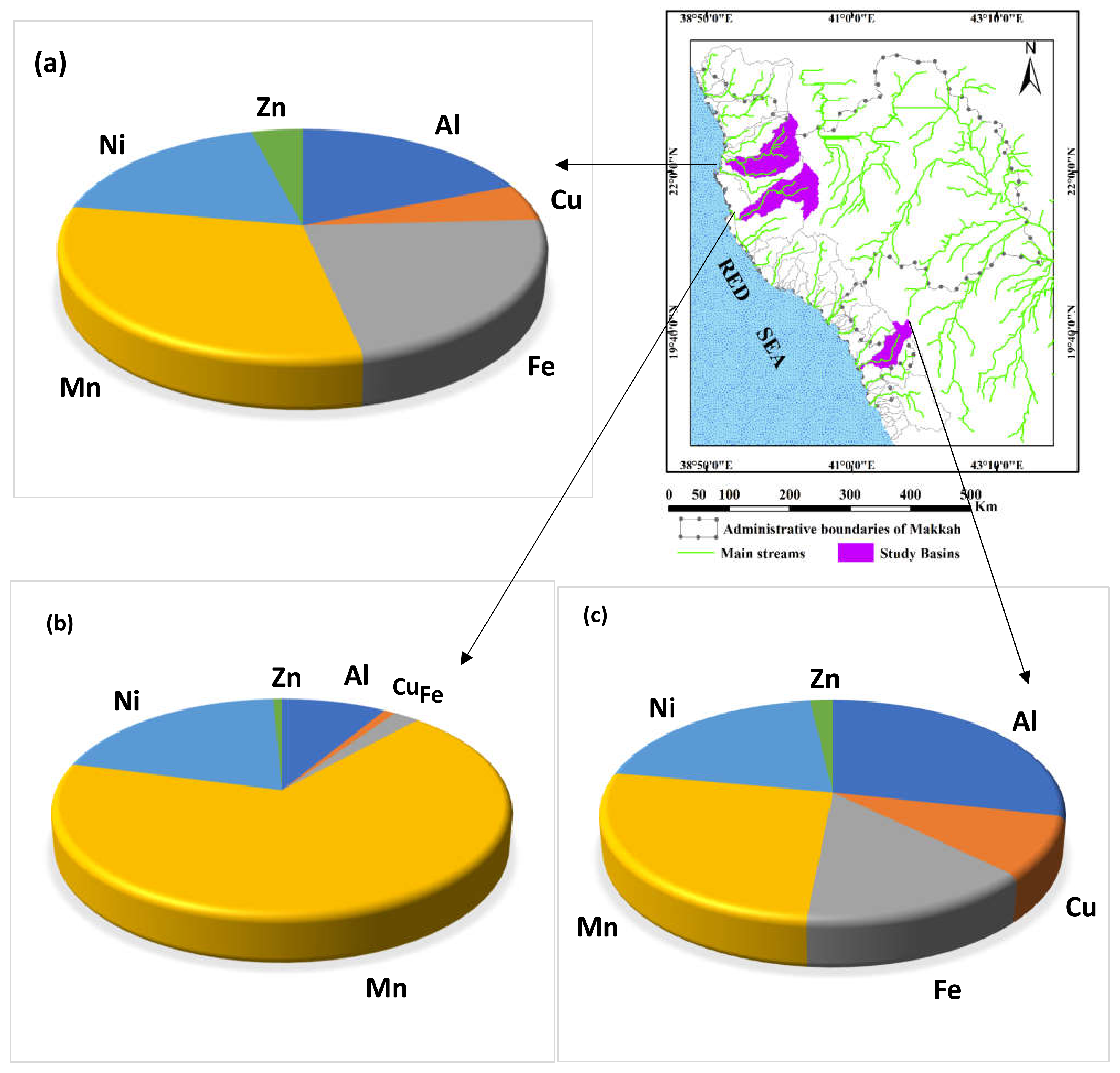
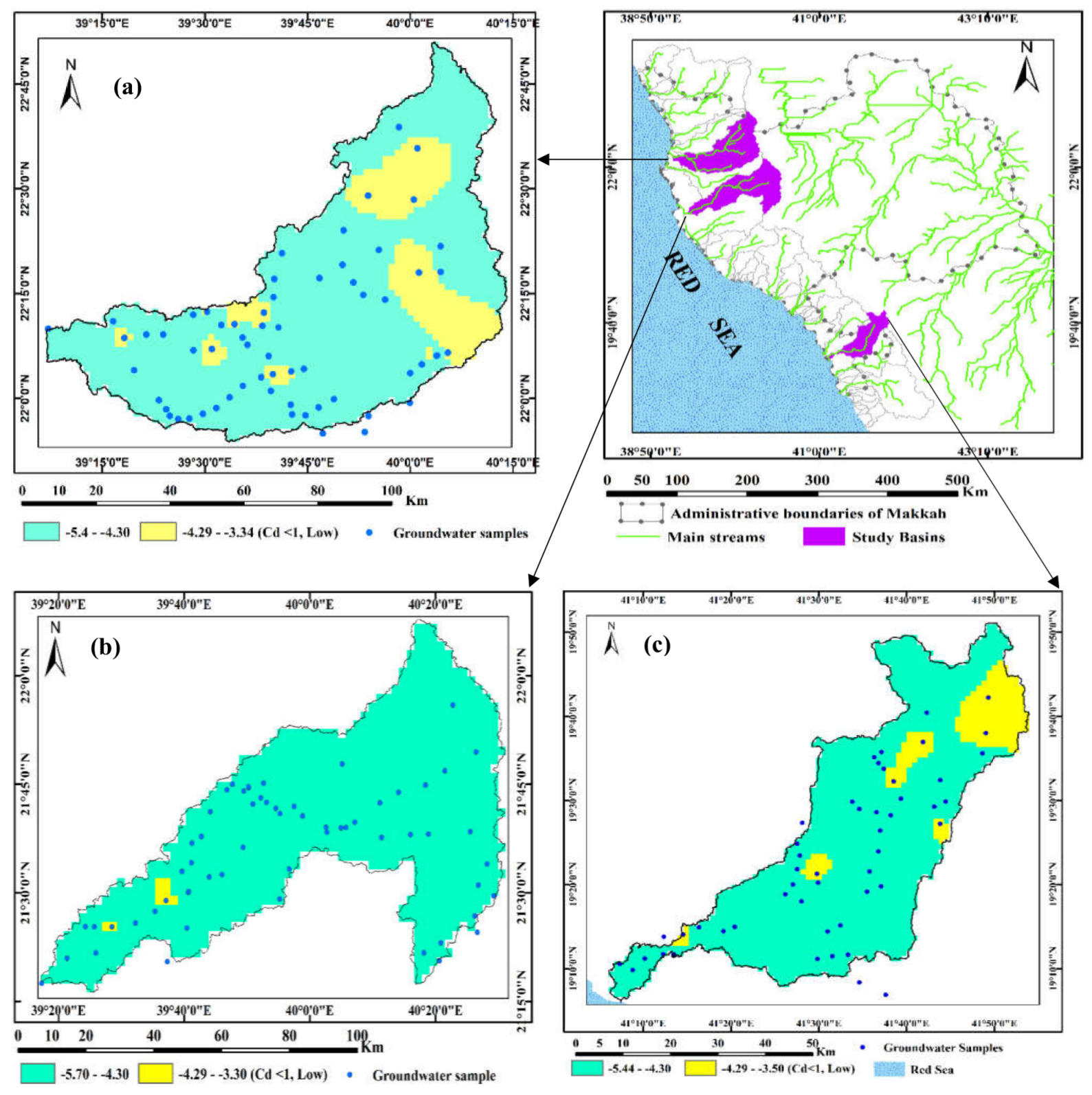
3.3.2. Pollution Indices (PIs)

Table 6 and Figure 9 showed statistical descriptions and classifications of groundwater samples with respect to PIs, such as HPI and C_d. The HPI readings varied from 5.07 to 77.41, with a mean value of 38.74, indicating that all groundwater points were less contaminated than the threshold HPI value (100). The calculated C_d values for the examined groundwater samples indicated that the C_d levels varied from −5.84 to −2.90, with a mean value of −5.02. The C_d values showed that all groundwater points had negative values (C_d < 1), suggesting a minimal degree of pollution and improved metal purity (Figure 10).

The PIs are regarded as an important technique for determining the appropriateness of water for drinking purposes in terms of metals [57]. According to the PIs findings, the majority of groundwater locations in the research region are not suitable for drinking. This might be attributable to a faulty drainage system, seawater intrusion, and rock–water interaction [20]. As a result, groundwater in the research region needs be treated before it can be consumed. The PIs, containing the HPI and C_d, demonstrated that groundwater in the wadies was low in metal contamination. According to the categorization of PI values, the data indicated two sets of heavy metal impacts (

Table 7. Groundwater quality assessment for the selected wadies in Makkah Al-Mukarramah Province based on metal impacts.

Metals	PI
	Wadi Marawani	Class	Effect	Wadi Fatimah	Class	Effect	Wadi Qanunah	Class	Effect
Al	0.58	I	No effect	0.18	I	No effect	0.58	I	No effect
Cu	0.16	I	No effect	0.02	I	No effect	0.18	I	No effect
Fe	0.69	I	No effect	0.04	I	No effect	0.29	I	No effect
Mn	0.96	I	No effect	1.43	II	Slight effect	0.54	I	No effect
Ni	0.56	I	No effect	0.43	I	No effect	0.41	I	No effect
Zn	0.12	I	No effect	0.02	I	No effect	0.04	I	No effect

and Figure 11). The obtained PI values demonstrated that metals had no influence on the groundwater points (PI < 1.0), whereas Mn had a slight effect in Wadi Fatimah (PI = 1–2), as shown in Table 7 and Figure 10. The PI results revealed two classes of heavy metal effects based on the classification of PI levels (Table 7 and Figure 11).

By comparing the geographical distribution maps of DWQI, HPI, and C_d findings, it is evident that the groundwater quality for drinking is deteriorating near the downstream parts of the wadies. Based on the link between the DWQI and PIs, metals had no effect on groundwater quality in the research regions. As a result of differences in heavy metal concentration measurement techniques, the groundwater quality in the study region revealed low levels of water contamination for HPI and C_d. As a result, combining the DWQI and PIs provides a beneficial and relevant technique for evaluating groundwater quality for drinking reasons using physiochemical parameters related to heavy metals.

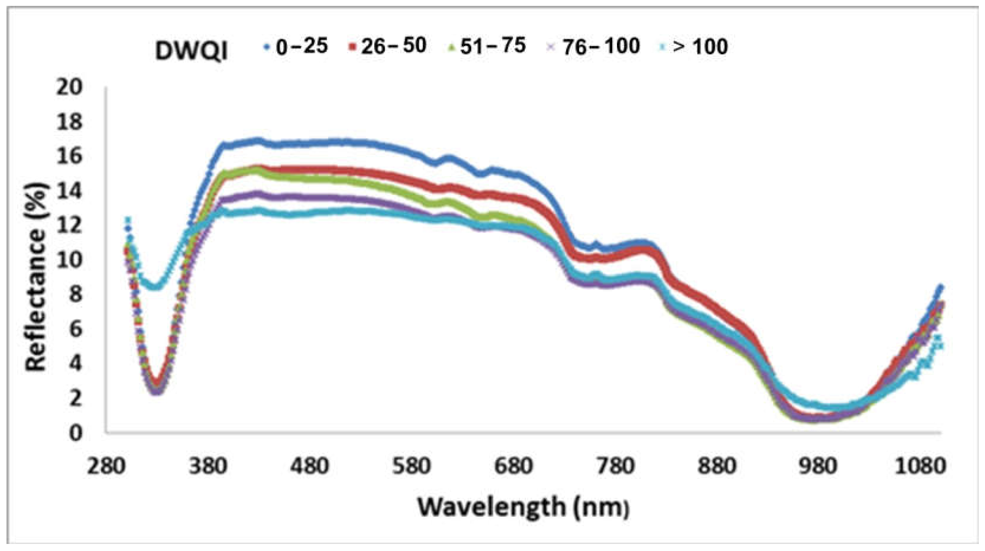
3.4. The Variation of Spectral Reflectance under Different Groundwater Quality Levels

The spectrum measurements for 173 groundwater samples collected in the three wadies were obtained. Figure 12 demonstrates the relationship between wavelength and reflectance at various DWQI levels across the three wadies. The results in Figure 12 show that there were distinct differences in respective spectral features associated to reflectance values throughout the VIS and NIR. From 800 to 850 nm, the combined form of the spectral signature and the wavelength locality exhibited a minor variation. The variance in spectra from blue to red (400–700 nm) indicated a higher difference than the NIR range (800–1148 nm). The spectral curve showed high values of reflectance at excellent levels of DWQI and low values of reflectance at unsuitable levels of DWQI. According to the data, the difference in spectral signature between DWQI levels, the VIS, and the NIR area is the highest among different electromagnetic spectrum regions. The difference in the composite form of the spectral signature produced at different DWQI levels appears to be a result of water component absorption. This conclusion emphasizes the importance of wavelength ranges in the VIS and NIR spectra in analyzing the three wadies’ WQIs. The properties of light reflected from water bodies at various wavebands in the magnetic spectrum can be utilized as markers of changes in the water physiochemical composition [36,37,58]. Surprisingly, these alterations result in considerable variations in the SRIs obtained from water samples throughout the whole spectral spectrum at certain bands. Several studies have found that the spectra at VIS, red-edge, and NIR have a stronger relationship with various physicochemical properties of different water bodies than other spectral regions, hinting that these spectral bands may be utilized to evaluate water quality [59,60,61,62,63,64,65,66].

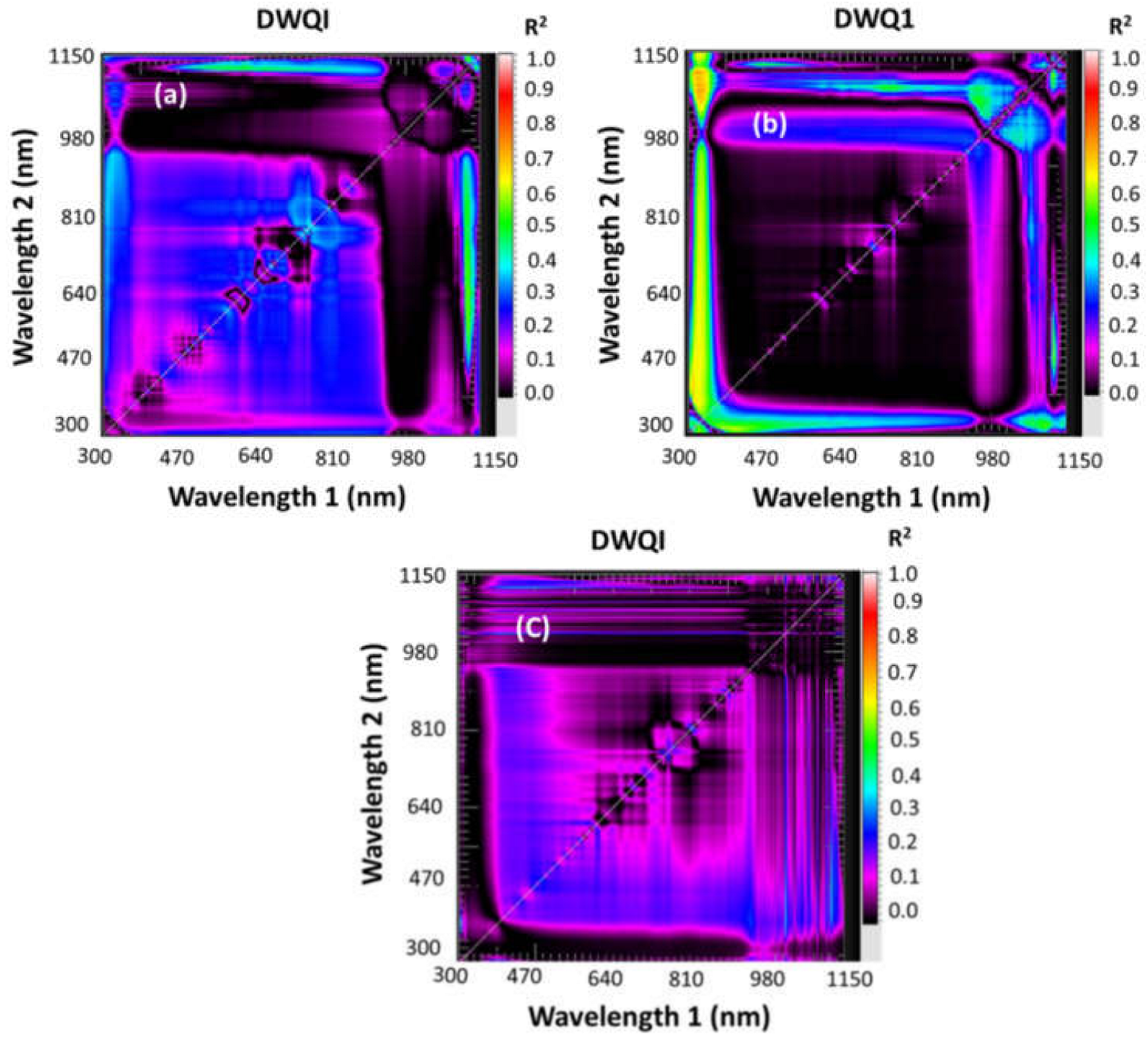
3.5. Performance of Different SRIs to Estimate Groundwater Quality Indices

Several studies have been carried out in order to investigate the effectiveness of optical remote sensing tools, such as satellite images and airborne and ground-based sensors, to estimate water quality levels. However, the majority of them have only investigated water quality metrics such as TSS, dissolved organic matter (DOM), chlorophyll-a, and turbidity [67,68,69,70,71,72,73]. However, a few studies employed nearby hyperspectra to determine the DWQI, HPI, and C_d of water [50]. The two-band slice map was used to pick R² for the associations between the four WQIs and the SRIs. The hotspot areas, depending on the color scale for the best R² based on information received from the WQIs in the VIS and NIR regions, were used to identify the best connections between the SRIs and WQIs. The hotspots (color scale) of the best R² identified were used to choose SRIs.

Table 8. Correlation coefficient of the linear association between SRIs and DWQI, TDS, HPI, and C_d.

	Wadi Marawani (n = 64)				Wadi Fatimah (n = 59)				Wadi Qanunah (n = 50)
	DWQI	TDS	HPI	Cd	DWQI	TDS	HPI	Cd	DWQI	TDS	HPI	Cd
B/R	0.46	0.46	−0.01	−0.21	−0.13	−0.13	0.13	−0.07	−0.44	−0.49	−0.12	0.07
G/R	0.49	0.49	−0.04	−0.25	−0.13	−0.14	0.09	−0.05	−0.39	−0.43	−0.11	0.07
NIR/R	−0.07	−0.03	−0.10	0.00	0.14	0.14	−0.21	−0.12	0.45	0.41	−0.05	−0.15
NIR/B	−0.40	−0.38	−0.03	0.17	0.11	0.11	−0.11	−0.02	0.50	0.52	0.09	−0.09
NIR/G	−0.38	−0.35	−0.03	0.17	0.12	0.12	−0.14	−0.03	0.48	0.47	0.04	−0.12
RSI1122,454	0.60	0.57	−0.25	−0.24	0.73	0.73	0.18	0.33	0.65	0.65	0.09	−0.04
RSI1122,470	0.66	0.63	−0.25	−0.25	0.76	0.76	0.18	0.34	0.65	0.64	0.08	−0.04
RSI1124,472	0.63	0.62	−0.15	−0.19	0.68	0.70	0.26	0.26	0.54	0.56	0.04	−0.12
RSI1122,480	0.69	0.66	−0.24	−0.26	0.75	0.75	0.18	0.33	0.65	0.63	0.08	−0.04
RSI1122,488	0.70	0.67	−0.24	−0.26	0.75	0.74	0.18	0.33	0.64	0.62	0.07	−0.04
RSI1122,510	0.73	0.71	−0.23	−0.27	0.71	0.71	0.17	0.30	0.63	0.60	0.06	−0.03
RSI1122,554	0.75	0.74	−0.20	−0.28	0.61	0.60	0.15	0.24	0.60	0.56	0.03	−0.03
RSI1124,570	0.74	0.74	−0.11	−0.23	0.44	0.45	0.21	0.13	0.49	0.48	−0.03	−0.14
RSI1122,590	0.75	0.74	−0.18	−0.29	0.48	0.48	0.15	0.19	0.56	0.52	0.03	−0.01

Note: All R values higher than −0.40 or 0.40 in table are significant.

shows the correlation coefficient (R) values for the association between the four measured WQIs and SRIs. Linear regression models demonstrated the significant relationships for the majority of SRIs paired with DWQI: R ranged from (−0.40 to 0.75), (0.44 to 0.76), and (−0.44 to 0.65); with TDS, R ranged from (0.46 to 0.74), (0.45 to 0.76), and (0.41 to 0.65) for Wadi Marawani, Wadi Fatimah, and Wadi Qanunah, respectively. This is due to the presence of different levels of drinking water quality, ranging from the level of excellent to the level of unsuitable for drinking.

New SRIs presented better performance for assessing the DWQI and TDS for three wadies than the published SRIs in Table 8. SRIs created using NIR and VIS regions, such as RSI_1122,590, RSI_1122,488, and RSI_1122,488, seem to be good indicators to assess DWQI and TDS. Wang et al., (2017) discovered that the DWQI may be easily detected at the peak wavelengths of 700–720 nm and 1070 nm. Spectrum curves for diverse water samples indicated multiple strong high absorbency zones at 700, 750, 950, and 980 nm, as well as low absorbency zones at 452, 703, and 850 nm, according to the researchers. Furthermore, Gad et al. [50] discovered that SRIs derived from the VIS and NIR regions had substantial associations with DWQI for two River Nile branches in Egypt. On the contrary, SRIs failed to assess both HPI and C_d, as the results of both indices suggested a minimal degree of pollution and improved metal purity. In addition, Gad et al. [50] found that SRIs could be used to assess metal index (MI) under different pollution levels.

3.6. Prediction of Different WQIs Using PLSR and PCR Models

SRIs are straightforward techniques for evaluating water quality and may be used to construct spectral sensors that are small and light for monitoring and controlling water quality on a broad scale in a timely and cost-effective way. However, each SRI focuses on just two or three sensitive waveband combinations [36,37]. This makes it challenging to construct effective SRIs for evaluating water quality under a number of potentially perplexing circumstances, such as large differences in water component amounts and types, as well as the impact of these differences on the saturation levels of the water quality measurements [42]. Therefore, in this work, the PLSR and PCR included SRIs as input variables to predict WQIs.

Table 9. Outcomes of calibration and validation models of PLSR for the association between observed and predicted values for DWQI, TDS, HPI, and C_d of the three wadies.

	Variable		Calibration			Validation
		LVs	R2	RMSE	Equation	R2	RMSE	Equation
Wadi Marawani	DWQI	6	0.69 ***	44.52	y = 0.6882x + 34.49	0.58 ***	52.29	y = 0.6323x + 41.862
	TDS	6	0.69 ***	1974.80	y = 0.6865x + 920.59	0.55 ***	2358.24	y = 0.631x + 1100.4
	HPI	1	0.05	9.01	y = 0.049x + 42.896	0.03	9.30	y = 0.0163x + 44.366
	Cd	4	0.18 *	0.53	y = 0.1753x − 3.9717	0.07	0.57	y = 0.1292x − 4.2123
Wadi Fatimah	DWQI	6	0.80 ***	38.74	y = 0.8041x + 23.252	0.75 ***	46.52	y = 0.7271x + 31.232
	TDS	7	0.84 ***	1296.72	y = 0.8378x + 417.3	0.77 ***	1555.53	y = 0.7739x + 529.15
	HPI	3	0.15 *	0.05	y = 0.1494x + 26.367	0.00	17.68	y = 0.0942x + 27.843
	Cd	1	0.10	0.44	y = 0.0998x − 4.8178	0.00	0.48	y = 0.0055x − 5.3217
Wadi Qanunah	DWQI	1	0.41 ***	15.46	y = 0.4111x + 32.043	0.42 ***	16.00	y = 0.3842x + 33.516
	TDS	1	0.40 ***	466.36	y = 0.3983x + 521.21	0.43 ***	484.43	y = 0.3689x + 541.47
	HPI	1	0.01	7.69	y = 0.0091x + 39.369	0.00	8.25	y = −0.0598x + 42.122
	Cd	1	0.01	0.55	y = 0.0088x − 4.8545	0.00	0.58	y = −0.0377x − 5.0867

Note: *, *** Statistically significant at p ≤ 0.05 and at p ≤ 0.001, respectively.

and

Table 10. Outcomes of calibration and validation models of PCR for the association between observed and predicted values for DWQI, TDS, HPI, and C_d of the three wadies.

	Variable	Calibration				Validation
		LVs	R2	RMSE	Equation	R2	RMSE	Equation
Wadi Marawani	DWQI	7	0.69 ***	44.26	y = 0.6918x + 34.082	0.60 ***	51.83	y = 0.6532x + 37.369
	TDS	7	0.69 ***	1965.51	y = 0.6894x + 911.96	0.60 ***	2321.90	y = 0.6325x + 1028.8
	HPI	1	0.03	9.10	y = 0.0294x + 43.781	0.01	9.36	y = 0.0015x + 45.056
	Cd	1	0.08	0.56	y = 0.0828x − 4.4171	0.05	0.58	y = 0.0527x − 4.5628
Wadi Fatimah	DWQI	6	0.80 ***	38.74	y = 0.8041x + 23.252	0.71 ***	46.70	y = 0.7034x + 34.53
	TDS	9	0.85 ***	1249.78	y = 0.8493x + 387.69	0.78 ***	1530.39	y = 0.7725x + 481.98
	HPI	1	0.05	17.31	y = 0.0468x + 29.547	0.03	17.92	y = 0.0117x + 30.655
	Cd	1	0.02	0.45	y = 0.0186x − 5.2524	0.01	0.46	y = 0.0039x − 5.3304
Wadi Qanunah	DWQI	1	0.41 ***	15.48	y = 0.4098x + 32.11	0.40 ***	16.04	y = 0.3819x + 33.581
	TDS	1	0.40 ***	467.15	y = 0.3963x + 522.98	0.37 ***	481.46	y = 0.3794x + 533.92
	HPI	1	0.01	7.70	y = 0.0045x + 39.55	0.00	8.15	y = −0.0514x + 41.847
	Cd	1	0.01	0.55	y = 0.0039x − 4.8781	0.00	0.57	y = −0.0252x − 5.0232

Note: *** Statistically significant at p ≤ 0.001.

describe the R² and RMSE, as well as the slope of equations of the two models used as criteria to estimate WQIs in Wadi Marawani, Wadi Fatimah, and Wadi Qanunah in Table 1. Generally, depend on these criteria, the PLSR and PCR models offered a more precise estimate of DWQI and TDS and failed to predict the HPI and C_d in Table 9 and Table 10. For example, The PLSR model produced reasonable DWQI and TDS estimations in calibration datasets with R² of 0.69 and 0.69, 0.80 and 0.84, and 0.41 and 0.40 in Wadi Marawani, Fatimah, and Qanunah, respectively (Table 10). The PLSR model produced reasonable DWQI and TDS estimations in validation datasets with R² of 0.60 and 0.60, 0.75 and 0.77, and 0.42 and 0.43 in Wadi Marawani, Fatimah, and Qanunah, respectively. The PCR model produced reasonable DWQI and TDS estimations in validation datasets with R² of 0.58 and 0.55, 0.71 and 0.78, and 0.40 and 0.37 in Wadi Marawani, Fatimah, and Qanunah, respectively (Table 10). In general, the PLSR and PCR models provided better estimation for DWQI and TDS than the indvidual SRI. The LVs ranged from 1 to 7 and were chosen to support the calibration data for the PLSR models of six WQIs without over-fitting through Wadi Marawani, Fatimah, and Qanunah (Table 9). In addition, the LVs ranged from 1 to 9 and were chosen to support the calibration data for the PCR models of six WQIs without over-fitting through Wadi Marawani, Fatimah, and Qanunah (Table 10). The optimal LVs was selected based on the lowest value of RMSE. Table 10 indicated variation in the slope of the linear relationship between measured and predicted values of PLSR models for each index, with TDS showing the highest slope (0.7739) and HPI showing the lowest slope (−0.0598). Furthermore, Table 10 indicated variation in the slope of the linear relationship between measured and predicted values of PCR models for each index, with TDS showing the highest slope (0.7725) and HPI showing the lowest slope (−0.0514). In both PLSR and PCR models, the RMSE value of each index was the smaller in Wadi Fatimah compare to the other two wadies. This is due to the presence of different levels of water quality between the three wadies.

Wang et al. [72] observed that PLSR models with a high number of wavebands outperformed models with only one or two wavebands in predicting inland water quality indices. In addition, Gad et al. [50] found that the PLSR model correctly predicted the DWQI and MI of the two branches of the River Nile in the validation datasets with R² varying from 0.78 to 0.93, respectively, under different levels of pollution. Again, PLSR and PCR models based on various SRIs may be used in water quality assessment as a unified strategy for remote WQI assessment.

4. Conclusions

The quality of groundwater in the Makkah region was investigated in this study to delineate the suitable zones for potable groundwater. The chemical analyses of the groundwater samples indicated that Na²⁺ > Ca²⁺ > Mg²⁺ > K⁺, Cl⁻ > SO₄²⁻ > HCO₃⁻ > NO₃⁻ > CO₃²⁻; and Cu > Fe > Al > Zn > Mn > Ni, respectively. The hydrochemical type of the groundwater samples revealed Ca-HCO₃, Na-Cl, mixed Ca-Mg-Cl-SO₄, and Na-Ca-HCO₃, which is controlled by seawater invasion, weathering process, and groundwater–rock interaction. The different WQIs, such as DWQI, HPI, C_d, and PI, were assessed for 173 groundwater samples. According to the DWQI assessment, the overall quality of groundwater samples in the studied areas varied greatly, from excellent (2.5%) to unfit for drinking (30.0%). The HPI, C_d, and PI values revealed that all groundwater samples had a low degree of contamination and were not affected by metals, except for Wadi Fatimah, which was slightly affected by Mn due to rock–water interaction. New SRIs derived from NIR and VIS, such as RSI_1122,590, RSI_1122,488, and RSI_1122,488, seem to be good indicators to assess DWQI and TDS. Generally, depending on R², RMSE, and slope values, the PLSR and PCR were more accurate in determining the DWQI and TDS and failed to predict the HPI and C_d. Finally, integrating WQIs, SRIs, PLSR, PCR, and GIS techniques was successful and provided a clear image for evaluating groundwater suitability for drinking and its regulating variables. In the future, the technique described in this work, which combines spectral indices algorithms and PLSR models, should be further assessed to increase its stability under varied groundwater resource conditions.

References

1. Pande, C.B.; Moharir, K.N.; Panneerselvam, B.; Singh, S.K.; Elbeltagi, A.; Pham, Q.B.; Varade, A.M.; Rajesh, J. Delineation of groundwater potential zones for sustainable development and planning using analytical hierarchy process (AHP), and MIF techniques. Appl. Water Sci. 2021, 11, 186. [Google Scholar] [CrossRef]
2. Pande, C.B.; Moharir, K.N.; Singh, S.K.; Elbeltagi, A.; Pham, Q.B.; Panneerselvam, B.; Panneerselvam, B.; Varade, A.M.; Kouadri, S. Groundwater flow modeling in the basaltic hard rock area of Maharashtra, India. Appl. Water Sci. 2022, 12, 12. [Google Scholar] [CrossRef]
3. Ramalingam, S.; Panneerselvam, B.; Kaliappan, S.P. Effect of high nitrate contamination of groundwater on human health and water quality index in semi-arid region, South India. Arab. J. Geosci. 2022, 15, 242. [Google Scholar] [CrossRef]
4. Benameur, T.; Benameur, N.; Saidi, N.; Tartag, S.; Sayad, H.; Agouni, A. Predicting factors of public awareness and perception about the quality, safety of drinking water, and pollution incidents. Environ. Monit. Assess. 2022, 194, 22. [Google Scholar] [CrossRef] [PubMed]
5. Ober, J.; Karwot, J. Tap Water Quality: Seasonal User Surveys in Poland. Energies 2021, 14, 3841. [Google Scholar] [CrossRef]
6. Mahler, R.L. Public perception trends of drinking water quality over a 32-year period in the Pacific Northwest, USA. Int. J. Environ. Impacts 2021, 4, 186–196. [Google Scholar] [CrossRef]
7. Elhdad, A.M. Assessment of surface water quality, raw versus treated, for different uses at Dakahlia Governorate, Egypt. Egypt. J. Chem. 2019, 62, 1117–1129. [Google Scholar] [CrossRef]
8. Zhang, Y.; Dai, Y.; Wang, Y.; Huang, X.; Xiao, Y.; Pei, Q. Hydrochemistry, quality and potential health risk appraisal of nitrate enriched groundwater in the Nanchong area, southwestern China. Sci. Total Environ. 2021, 784, 147186. [Google Scholar] [CrossRef]
9. Gad, M.; El Osta, M. Geochemical controlling mechanisms and quality of the groundwater resources in El Fayoum Depression, Egypt. Arab. J. Geosci. 2020, 13, 861. [Google Scholar] [CrossRef]
10. Li, C.; Gao, X.; Li, S.; Bundschuh, J. A review of the distribution, sources, genesis, and environmental concerns of salinity in groundwater. Environ. Sci. Pollut. Res. 2020, 27, 41157–41174. [Google Scholar] [CrossRef]
11. Vespasiano, G.; Muto, F.; Apollaro, C. Geochemical, geological and groundwater quality characterization of a complex geological framework: The case study of the Coreca area (Calabria, South Italy). Geosciences 2021, 11, 121. [Google Scholar] [CrossRef]
12. Zhou, Y.; Li, P.; Xue, L.; Dong, Z.; Li, D. Solute geochemistry and groundwater quality for drinking and irrigation purposes: A case study in Xinle City, North China. Geochemistry 2020, 80, 125609. [Google Scholar] [CrossRef]
13. Panneerselvam, B.; Muniraj, K.; Duraisamy, K.; Pande, C.; Karuppannan, S. An integrated approach to explore the suitability of nitrate-contaminated groundwater for drinking purposes in a semiarid region of India. Environ. Geochem. Health 2022, 3, 1–17. [Google Scholar] [CrossRef]
14. He, S.; Li, P.; Wu, J.; Elumalai, V.; Adimalla, N. Groundwater quality under land use/land cover changes: A temporal study from 2005 to 2015 in Xi’an, Northwest China. Hum. Ecol. Risk Assess. Int. J. 2020, 26, 2771–2797. [Google Scholar] [CrossRef]
15. Adimalla, N.; Qian, H.; Li, P. Entropy water quality index and probabilistic health risk assessment from geochemistry of groundwaters in hard rock terrain of Nanganur County, South India. Geochemistry 2020, 80, 125544. [Google Scholar] [CrossRef]
16. Gad, M.; El-Hattab, M. Integration of water pollution indices and DRASTIC model for assessment of groundwater quality in El Fayoum Depression, western desert, Egypt. J. Afr. Earth Sci. 2019, 158, 103554. [Google Scholar] [CrossRef]
17. Adimalla, N. Application of the Entropy Weighted Water Quality Index (EWQI) and the Pollution Index of Groundwater (PIG) to Assess Groundwater Quality for Drinking Purposes: A Case Study in a Rural Area of Telangana State, India. Arch. Environ. Contam. Toxicol. 2021, 80, 31–40. [Google Scholar] [CrossRef]
18. Hasan, M.S.U.; Rai, A.K. Groundwater quality assessment in the Lower Ganga Basin using entropy information theory and GIS. J. Clean. Prod. 2020, 274, 123077. [Google Scholar] [CrossRef]
19. Liu, J.; Peng, Y.; Li, C.; Gao, Z.; Chen, S. Characterization of the hydrochemistry of water resources of the Weibei Plain, Northern China, as well as an assessment of the risk of high groundwater nitrate levels to human health. Environ. Pollut. 2021, 268, 115947. [Google Scholar] [CrossRef]
20. Wu, C.; Wu, X.; Qian, C.; Zhu, G. Hydrogeochemistry and groundwater quality assessment of high fluoride levels in the Yanchi endorheic region, northwest China. Appl. Geochem. 2018, 98, 404–417. [Google Scholar] [CrossRef]
21. Shamshirband, S.; Jafari Nodoushan, E.; Adolf, J.E.; Abdul Manaf, A.; Mosavi, A.; Chau, K.W. Ensemble models with uncertainty analysis for multi-day ahead forecasting of chlorophyll a concentration in coastal waters. Eng. Appl. Comput. Fluid Mech. 2018, 13, 91–101. [Google Scholar] [CrossRef] [Green Version]
22. Tiyasha, T.M.; Yaseen, Z.M. A survey on river water quality modelling using artificial intelligence models: 2000–2020. J. Hydrol. 2020, 585, 124670. [Google Scholar] [CrossRef]
23. Kumar, R.; Singh, S.; Bilga, P.S.; Jatin, S.J.; Singh, S.; Scutaru, M.L.; Pruncu, C.I. Revealing the benefits of entropy weights method for multi-objective optimization in machining operations: A critical review. J. Mater. Res. Technol. 2021, 10, 1471–1492. [Google Scholar] [CrossRef]
24. Adimalla, N.; Taloor, A.K. Hydrogeochemical investigation of groundwater quality in the hard rock terrain of South India using Geographic Information System (GIS) and groundwater quality index (GWQI) techniques. Groundw. Sustain. Dev. 2020, 10, 100288. [Google Scholar] [CrossRef]
25. Dimri, D.; Daverey, A.; Kumar, A.; Sharma, A. Monitoring water quality of river ganga using multivariate techniques and WQI (water quality index) in western himalayan region of uttarakhand, India. Environ. Nanotechnol. Monit. Manag. 2021, 15, 100375. [Google Scholar] [CrossRef]
26. Pak, H.Y.; Chuah, C.J.; Tan, M.L.; Yong, E.L.; Snyder, S.A. A framework for assessing the adequacy of Water Quality Index—Quantifying parameter sensitivity and uncertainties in missing values distribution. Sci. Total Environ. 2021, 751, 141982. [Google Scholar] [CrossRef]
27. Taloor, A.K.; Pir, R.A.; Adimalla, N.; Ali, S.; Manhas, D.S.; Roy, S.; Singh, A.K. Spring water quality and discharge assessment in the Basantar watershed of Jammu Himalaya using geographic information system (GIS) and water quality Index (WQI). Groundw. Sustain. Dev. 2020, 10, 100364. [Google Scholar] [CrossRef]
28. Uddin, M.G.; Nash, S.; Olbert, A.I. A review of water quality index models and their use for assessing surface water quality. Ecol. Indic. 2021, 122, 107218. [Google Scholar] [CrossRef]
29. El-Gammal, M.; Ibrahim, M.; El-Sonbati, M.; El-Zeiny, A. Assessment of Heavy Metal Contamination on Street Dust at New Damietta City, Egypt. J. Environ. Sci. 2011, 40, 221–237. [Google Scholar]
30. El-Alfy, M.A.; Hasballah, A.F.; Abd El-Hamid, H.T.; El-Zeiny, A.M. Toxicity assessment of heavy metals and organochlorine pesticides in freshwater and marine environments, Rosetta area, Egypt using multiple approaches. Sustain. Environ. Res. 2019, 29, 12. [Google Scholar] [CrossRef] [Green Version]
31. El-Zeiny, A.M.; El Kafrawy, S.B.; Ahmed, M.H. Geomatics based approach for assessing Qaroun Lake pollution, Egypt. J. Remote Sens. Space Sci. 2019, 22, 279–296. [Google Scholar]
32. Shareef, M.A.; Khenchaf, A.; Toumi, A. Integration of passive and active microwave remote sensing to estimate water quality parameters. In Proceedings of the IEEE Radar Conference, Philadelphia, PA, USA, 2–6 May 2016; pp. 1–4. [Google Scholar]
33. Yang, Y.; Gao, B.; Hao, H.; Zhou, H.; Lu, J. Nitrogen and phosphorus in sediments in China: A national-scale assessment and review. Sci. Total Environ. 2017, 576, 840–849. [Google Scholar] [CrossRef] [PubMed]
34. Gad, M.; El-Hendawy, S.; Al-Suhaibani, N.; Tahir, M.U.; Mubushar, M.; Elsayed, S. Combining Hydrogeochemical Characterization and a Hyperspectral Reflectance Tool for Assessing Quality and Suitability of Two Groundwater Resources for Irrigation in Egypt. Water 2020, 12, 2169. [Google Scholar] [CrossRef]
35. El Osta, M.; Masoud, M.; Alqarawy, A.; Elsayed, S.; Gad, M. Groundwater Suitability for Drinking and Irrigation UsingWater Quality Indices and Multivariate Modeling in Makkah Al-Mukarramah Province, Saudi Arabia. Water 2022, 14, 483. [Google Scholar] [CrossRef]
36. Elsayed, S.; Gad, M.; Farouk, M.; Saleh, A.H.; Hussein, H.; Elmetwalli, A.H.; Elsherbiny, O.; Moghanm, F.S.; Moustapha, M.E.; Taher, M.A.; et al. Using Optimized Two and Three-Band Spectral Indices and Multivariate Models to Assess Some Water Quality Indicators of Qaroun Lake in Egypt. Sustainability 2021, 13, 10408. [Google Scholar] [CrossRef]
37. Elsayed, S.; Ibrahim, H.; Hussein, H.; Elsherbiny, O.; Elmetwalli, A.H.; Moghanm, F.S.; Ghoneim, A.M.; Danish, S.; Datta, R.; Gad, M. Assessment of Water Quality in Lake Qaroun Using Ground-Based Remote Sensing Data and Artificial Neural Networks. Water 2021, 13, 3094. [Google Scholar] [CrossRef]
38. Sharaf, M.A.M. Major elements hydrochemistry and groundwater quality of Wadi Fatimah, West Central Arabian Shield, Saudi Arabia. Arab. J. Geosci. 2021, 6, 2633–2653. [Google Scholar] [CrossRef]
39. Al-Ahmadi, M.E.; El-Fiky, A.A. Hydrogeochemical evaluation of shallow alluvial aquifer of Wadi Marwani, western Saudi Arabia. J. King Saud Univ. Sci. 2009, 21, 179–190. [Google Scholar] [CrossRef] [Green Version]
40. Al-Gadi, K.; Al-Doaan, M. Seawater intrusion into groundwater costal aquifers at AL-Qunfudah province, Western Saudi Arabia. Multi-Knowl. Electron. Compr. J. Educ. Sci. Publ. 2020, 31, 22. [Google Scholar]
41. APHA (American Public Health Association). Standard Methods for the Examination of Water and Wastewater; American Public Health Association: Washington, DC, USA, 2012. [Google Scholar]
42. Khadr, M.; Gad, M.; El-Hendawy, S.; Al-Suhaibani, N.; Dewir, Y.H.; Tahir, M.U.; Mubushar, M.; Elsayed, S. The Integration of Multivariate Statistical Approaches, Hyperspectral Reflectance, and Data-Driven Modeling for Assessing the Quality and Suitability of Groundwater for Irrigation. Water 2021, 13, 35. [Google Scholar] [CrossRef]
43. Chipman, J.W.; Olmanson, L.G.; Gitelson, A.A. Remote Sensing Methods for Lake Management: A Guide for Resource Managers and Decision-Makers; North American Lake Management Society: Madison, WI, USA, 2009. [Google Scholar]
44. Somvanshi, S.; Kunwar, P.; Singh, N.; Shukla, S.; Pathak, V. Integrated remote sensing and GIS approach for water quality analysis of gomti river, Uttar Pradesh. Int. J. Environ. Sci. 2012, 3, 62–74. [Google Scholar]
45. Bhatti, A.M.; Nasu, S.; Takagi, M.; Nojiri, Y. Assessing the potential of remotely sensed data for water quality monitoring of coastal and inland waters. Res. Bull. Kochi Univ. Technol. 2008, 5, 201–207. [Google Scholar]
46. Brown, R.M.; McCleiland, N.J.; Deininger, R.A.; O’Connor, M.F. A Water Quality Index—Crossing the Psychological Barrier. In Proceedings of the 2nd International Conference on Water Pollution Research, Jerusalem, Israel, 18–24 June 1972; Volume 6, pp. 787–797. [Google Scholar]
47. Prasad, B.; Bose, J.M. Evaluation of heavy metal pollution index for surface and spring water near a limestone mining area of the Lower Himalayas. Environ. Geol. 2001, 41, 183–188. [Google Scholar] [CrossRef]
48. Edet, A.E.; Offong, O.E. Evaluation of water quality pollution indices for heavy metal contamination monitoring. A study case from Akpabuyo-Odukpani area, Lower Cross River Basin (South Nigeria). GeoJournal 2002, 4, 295–304. [Google Scholar] [CrossRef]
49. Caerio, S.; Costa, M.H.; Ramos, T.B.; Fernandes, F.; Silveira, N.; Coimbra, A.; Painho, M. Assessing heavy metal contamination in Sado Estuary sediment: An index analysis approach. Ecol. Indic. 2005, 5, 155–169. [Google Scholar] [CrossRef]
50. Gad, M.; Saleh, A.H.; Hussein, H.; Farouk, M.; Elsayed, S. Appraisal of Surface Water Quality of Nile River Using Water Quality Indices, Spectral Signature and Multivariate Modeling. Water 2022, 14, 1131. [Google Scholar] [CrossRef]
51. WHO (World Health Organization). Guidelines for Drinking-Water Quality, 4th ed.; Incorporating the 1st Addendum; WHO: Geneva, Switzerland, 2011. [Google Scholar]
52. Khan, R.; Saxena, A.; Shukla, S.; Sekar, S.; Senapathi, V.; Wu, J. Environmental contamination by heavy metals and associated human health risk assessment: A case study of surface water in Gomti River Basin, India. Environ. Sci. Pollut. Res. 2021, 28, 56105–56116. [Google Scholar] [CrossRef]
53. Nasrabadi, T. An index approach to metallic pollution in river waters. Int. J. Environ. Res. 2015, 9, 385–394. [Google Scholar]
54. Goher, M.E.; Farhat, H.I.; Abdo, M.H.; Salem, S.G. Metal pollution assessment in the surface sediment of Lake Nasser, Egypt. Egypt. J. Aquat. Res. 2014, 40, 213–224. [Google Scholar] [CrossRef] [Green Version]
55. Piper, A.M. A graphic procedure in the geochemical interpretation of water-analyses. EOS Trans. Am. Geophys. Union 1944, 25, 914–928. [Google Scholar] [CrossRef]
56. Gibbs, R.J. Mechanisms controlling world water chemistry. Science 1970, 170, 1088–1090. [Google Scholar] [CrossRef]
57. Kachroud, M.; Trolard, F.; Kefi, M.; Jebari, S.; Bourrie, G. Water quality indices: Challenges and application limits in the literature. Water 2019, 11, 361. [Google Scholar] [CrossRef] [Green Version]
58. Maliki, A.A.A.; Chabuk, A.; Sultan, M.A.; Hashim, B.M.; Hussain, H.M.; Al-Ansari, N. Estimation of total dissolved solids in water bodies by spectral indices Case Study: Shatt al-Arab River. Water Air Soil Pollut. 2020, 231, 482. [Google Scholar] [CrossRef]
59. Seyhan, E.; Dekker, A. Application of remote sensing techniques for water quality monitoring. Hydrol. Biol. Bull. 1986, 20, 41–50. [Google Scholar] [CrossRef]
60. Shafique, N.A.; Autrey, B.C.; Fulk, F.; Cormier, S.M. Hyperspectral narrow wavebands selection for optimizing water quality monitoring on the Great Miami River, Ohio. J. Spat. Hydrol. 2001, 1, 1–22. [Google Scholar]
61. El-Din, M.S.; Gaber, A.; Koch, M.; Ahmed, R.S.; Bahgat, I. Remote sensing application for water quality assessment in lake timsah, Suez Canal, Egypt. J. Remote Sens. Technol. 2013, 1, 61–74. [Google Scholar] [CrossRef]
62. Wu, J.L.; Ho, C.R.; Huang, C.C.; Srivastav, A.L.; Tzeng, J.H.; Lin, Y.T. Hyperspectral sensing for turbid water quality monitoring in freshwater rivers: Empirical relationship between reflectance and turbidity and total solids. Sensors 2014, 14, 22670–22688. [Google Scholar] [CrossRef] [Green Version]
63. Lerch, R.N.; Baffaut, C.; Kitchen, N.R.; Sadler, E.J. Long-term agroecosystem research in the Central Mississippi River Basin: Dissolved nitrogen and phosphorus transport in a high-runoff-potential watershed. J. Environ. Qual. 2015, 44, 44–57. [Google Scholar] [CrossRef]
64. Wang, Z.; Kawamura, K.; Sakuno, Y.; Fan, X.; Gong, Z.; Lim, J. Retrieval of chlorophyll-a and total suspended solids using iterative stepwise elimination partial least squares (ISE-PLS) regression based on field hyperspectral measurements in irrigation ponds in Higashihiroshima, Japan. Remote Sens. 2017, 9, 264. [Google Scholar] [CrossRef] [Green Version]
65. Elhag, M.; Gitas, I.; Othman, A.; Bahrawi, J.; Gikas, P. Assessment of water quality parameters using temporal remote sensing spectral reflectance in arid environments, Saudi Arabia. Water 2019, 11, 556. [Google Scholar] [CrossRef] [Green Version]
66. Xing, Z.; Chen, J.; Zhao, X.; Li, Y.; Li, X.; Zhang, Z.; Lao, C.; Wang, H. Quantitative estimation of wastewater quality parameters by hyperspectral band screening using GC, VIP and SPA. PeerJ 2019, 7, 8255. [Google Scholar] [CrossRef] [PubMed] [Green Version]
67. Duan, W.; He, B.; Takara, K.; Luo, P.; Nover, D.; Sahu, N.; Yamashiki, Y. Spatiotemporal evaluation of water quality incidents in Japan between 1996 and 2007. Chemosphere 2013, 93, 946–953. [Google Scholar] [CrossRef] [PubMed]
68. Vinciková, H.; Hanuš, J.; Pechar, L. Spectral reflectance is a reliable water-quality estimator for small, highly turbid wetlands. Wetlands Ecol. Manag. 2015, 23, 933–946. [Google Scholar] [CrossRef]
69. Gholizadeh, M.H.; Melesse, A.M.; Reddi, L.A. A Comprehensive review on water quality parameters estimation using remote sensing techniques. Sensors 2016, 16, 1298. [Google Scholar] [CrossRef] [Green Version]
70. Xiao, R.; Wang, G.; Zhang, Q.; Zhang, Z. Multi-scale analysis of relationship between landscape pattern and urban river water quality in different seasons. Sci. Rep. 2016, 6, 25250. [Google Scholar] [CrossRef] [Green Version]
71. Deng, Y.; Zhang, Y.; Li, D.; Shi, K.; Zhang, Y. Temporal and spatial dynamics of phytoplankton primary production in Lake Taihu derived from MODIS data. Remote Sens. 2017, 9, 195. [Google Scholar] [CrossRef]
72. Wang, X.; Zhang, F.; Ding, J. Evaluation of water quality based on a machine learning algorithm and water quality index for the Ebinur Lake Watershed, China. Sci. Rep. 2017, 7, 12858. [Google Scholar] [CrossRef] [Green Version]
73. Zhang, Y.; Giardino, C.; Li, L. Water optics and water colour remote sensing. Remote Sens. 2017, 9, 818. [Google Scholar] [CrossRef] [Green Version]
Figure 1. Location map of the groundwater points for the selected wadies in Makkah Al-Mukarramah Province, Saudi Arabia: (a) Wadi Marawani, (b) Wadi Fatimah, and (c) Wadi Qanunah.
Water 14 02311 g001
Figure 2. (a) Digital elevation model (DEM) and (b) geological map of Makkah Al-Mukarramah Province, Saudi Arabia.
Water 14 02311 g002
Figure 3. Annual distribution map of average rainfall (mm) in Makkah Al-Mukarramah Province, Saudi Arabia (1960–2012).
Water 14 02311 g003
Figure 4. Correlation matrices displaying (R2) values for possible dull wavelength ranging from 302 to 1148 nm with DWQI of three wadies: (a) Wadi Marawani, (b) Wadi Fatimah, and (c) Wadi Qanunah.
Water 14 02311 g004
Figure 5. Schematic flowchart of the process of PLSR and PCR used to assess DWQI, TDS, HPI, and Cd of water samples in this study.
Water 14 02311 g005
Figure 6. Geochemical facies and water type for selected wadies: (a) Wadi Marawani, (b) Wadi Fatimah, and (c) Wadi Qanunah, Makkah Al-Mukarramah Province.
Water 14 02311 g006
Figure 7. Geochemical controlling mechanisms for selected wadies: (a) Wadi Marawani, (b) Wadi Fatimah, and (c) Wadi Qanunah, Makkah Al-Mukarramah Province.
Water 14 02311 g007
Figure 8. Spatial distribution map of DWQI for selected wadies: (a) Wadi Marawani, (b) Wadi Fatimah, and (c) Wadi Qanunah, Makkah Al-Mukarramah Province.
Water 14 02311 g008
Figure 9. Spatial distribution map of HPI for selected wadies: (a) Wadi Marawani, (b) Wadi Fatimah, and (c) Wadi Qanunah, Makkah Al-Mukarramah Province.
Water 14 02311 g009
Figure 10. Spatial distribution map of Cd for selected wadies: (a) Wadi Marawani, (b) Wadi Fatimah, and (c) Wadi Qanunah, Makkah Al-Mukarramah Province.
Water 14 02311 g010
Figure 11. Three-dimensional pie showing the relative pollution index of metals for selected wadies: (a) Wadi Marawani, (b) Wadi Fatimah, and (c) Wadi Qanunah, Makkah Al-Mukarramah Province.
Water 14 02311 g011
Figure 12. Spectra reflectance of the various levels of drinking groundwater quality index across the three wadies samples.
Water 14 02311 g012