Abstract
Although soil water redistribution is critical for a number of problems, a rather limited study of this process has been reported up to now and especially as regards the implications of hysteresis on horizontal soil water redistribution after infiltration. To this end, a thorough theoretical and numerical investigation of the redistributed soil water content profiles formed after the cessation of a horizontal infiltration is presented. A number of different initial soil water contents before the initiation of the horizontal infiltration and different infiltration depths were analyzed using the HYDRUS-1D software package considering the appropriate hysteretic wetting and drying curves. The effect of neglecting hysteresis was also investigated for the same conditions. The main wetting and drying boundary curves of the studied porous medium and the hydraulic conductivity at saturation were experimentally determined. The theoretical and numerical analysis indicated that the form of the redistributed soil water content profiles in the presence of hysteresis was similar to the original infiltration profile independently of whether the initial soil water content was taken on the boundary wetting or drying curve and independently of the porous medium type. Specifically, in a relatively short time after the initiation of the redistribution process, the magnitude of the soil matrix head gradient tended to zero due to hysteresis, and this resulted in an insignificant soil water movement, although the soil water content and the hydraulic conductivity values were still high. In addition, the redistribution proceeded at a faster rate than the smallest depth of infiltration water prior to the redistribution, and it was faster during the early stages of the redistribution. Accordingly, hysteresis is important for the simulation of horizontal soil water redistribution as it is, for example, in the case of localized irrigation systems’ design and management.
1. Introduction
Soon after every irrigation event, soil water redistribution takes place, which causes soil water from the upper soil layer to move further down, thus reducing soil moisture from this layer and increasing it for the layers below, beyond the initial soil water front achieved during the original infiltration. In other words, the phenomenon of drainage occurs at the upper soil layer, while at the same time, wetting continues to occur at lower soil layers. During the redistribution process, for the area where drainage takes place, the relationship between soil water pressure head (H), soil water content (θ), and hydraulic conductivity (K) in every point would be described by the respective drying scanning curve, which would be different for every point in the soil profile. For this drainage process, H is not a unique function of θ, but its value in a certain point x depends also on the value of θ at the reversal from wetting to drying. For the area where wetting occurs during redistribution, if the soil column had initially a relatively uniform small value of θ, then the relationship between H, θ, and K would be given by the boundary wetting curve or an appropriate wetting scanning curve.
Although soil water redistribution is actually responsible for the soil moisture profile establishment in the root zone, and its serious study would be helpful in facing a number of problems concerning the evaluation of various soil water quantities and their salt contents, moving in and out of the plant root zone [1,2], a rather restricted study of this process has been reported in relation to the infiltration problem [3]. The basic obstacle for this is the involvement of the phenomenon of hysteresis, characterizing the relationships of the soil hydraulic properties, and especially between H and θ, thus making the redistribution process very difficult to study and manage.
Youngs [4] presented experimental horizontal redistribution profiles supporting that the introduction of diffusivity, D, in Richards’ equation cannot be used in the case of redistribution after infiltration when hysteresis is involved. Youngs and Poulovassilis [5], based on the classical theory of soil water movement, showed evidence that during the redistribution process, after a vertical infiltration event, two distinct forms of soil water profiles could appear. Which form would appear each time depended on the depth to which the soil water had been infiltrated and also on the value of the soil water pressure head gradient compared to the gradient of the gravity.
In this respect, the first form of the redistribution profile keeps approximately the infiltration profile shape, when the gravity gradient is small compared to that of the soil water pressure head gradient, and the redistribution rate is higher when the soil water depth being infiltrated is small. Profiles of such forms are anticipated to appear, in the case of fine porous media when the soil water depth originally infiltrated is small and also in the case of the horizontal redistribution after infiltration. In the second form, desaturation at the surface occurs with a step-like advancement of the wetting front below, while the redistribution rate is proportionally related to the infiltration depth and is anticipated to appear in the redistribution process for large values of the originally infiltrated soil water depths and for coarser porous media. Youngs [6] presented a different approach concerning the development of the redistribution profiles using scaling based on similar media theory.
Poulovassilis [7] investigated the effect of the initial water content prevailing in a porous column before the initiation of the vertical infiltration in the subsequent redistribution of the soil water and showed that the redistribution rate for initial states on the boundary drying curve is greater than that for states on the boundary wetting curve. Moreover, it has been reported that an increase in the initial water content along the boundary drying curve may lead to an increase in the redistribution rate, while an increase in initial water content along the boundary wetting curve may lead to a decrease in the redistribution rate.
Philip [3] studied a special case of the horizontal redistribution, where the porous medium along the horizontal column was uniform but the initial water content along the soil column differed between the left and the right part of the column and developed a similarity solution describing horizontal redistribution among the two semi-infinite halves of an infinite column. The accurate and relatively simple analysis and the solution of the specific problem of soil water content redistribution in a horizontal soil column presented by Philip [3] concluded that the resorptivity R is analogous to the sorptivity S, and its value was approximately 1/3 of S; additionally, R was affected very little by hysteresis. Moreover, between the two regions, the water content profiles during the redistribution presented quite different characteristics. In the region where desorption occurs, the water content profiles were gradual with a large extent of penetration depth, while in the region of absorption, the water content profiles appeared to be more abrupt and the penetration depth small.
Heinen and Raats [8], following the work of Philip [3], studied all the possible cases of the horizontal redistribution in a horizontal uniform soil column with the help of a numerical simulation model. Depending on the initial conditions in two parts of an infinitely long soil column, it was demonstrated that three distinct behaviors can be observed: no flow, conventional flow from the wet part to the dry part, or unconventional flow from the dry part to the wet part. Heinen and Raats [8], in order to consider the phenomenon of hysteresis in the H, θ, and K relationships, made use of the Mualem [9] model. However, this particular case of redistribution does not address the realistic complex hysteretic soil behavior of soils during the infiltration/redistribution cycle, when different parts of the soil profile are wetting and drying following the corresponding wetting and drying scanning curves [10]. Zhuang et al. [11] made use of two different approaches in their attempt to analyze data from a horizontal redistribution case of the form that Philip [3] had examined. Their approaches included the classical application of the Richards’ equation, taking into consideration the hysteretic relationship between H and θ, and the other one was based on principles of thermodynamics. For the simulation, concerning the first case, the HYDRUS-1D model was used, for which the appropriate wetting and drying scanning curves were calculated according to the approach of Lenhard et al. [12]. Their results indicated that the application of Richards’ equation in the presence of hysteresis describes the discontinuity of θ at the interface between the wet and dry sections of a horizontal soil column immediately after they are come into contact but predicts higher redistribution rates and higher θ values at the dry section.
Various theoretical and empirical models, describing the hysteretic relationships of the hydraulic properties (H, θ και Κ) of the porous medium, have been proposed to date [9,13,14,15,16,17]. Moreover, a number of research works have presented comparisons between models and also comparisons between models and actual experimental data [18,19,20].
A number of numerical simulation models have been proposed for solving the one-dimensional problem of infiltration–redistribution. Among them, HYDRUS-1D [21] is the one most widely applied. HYDRUS-1D gives the possibility of including the hysteretical nature of the soil hydraulic properties, as these are expressed by various empirical models [12,22]. Specifically, for the horizontal redistribution case with the inclusion of the hysteresis process, the HYDRUS 1-D has been only applied for the special case where two soil samples with the same hydraulic properties but different initial water saturations are brought into contact [11].
The above analysis reveals that while the issue of soil water redistribution in the case of vertical infiltration has been extensively studied for a wide set of conditions, it has been only fragmentary studied as regards horizontal infiltration and only for peculiar conditions. Accordingly, a more holistic investigation of the phenomenon of horizontal soil water redistribution after initial application of infiltration is still lacking and especially concerning the implications of hysteresis.
In this context, the main objective of this study was to provide a more thorough theoretical and numerical analysis of the soil water redistribution after the cessation of horizontal infiltration. To this end, a detailed theoretical analysis was carried out, and the redistributed soil water content profiles formed after the cessation of horizontal infiltration were numerically investigated with the help of HYDRUS-1D software package. A wide range of combinations of different original infiltration times (corresponding to different infiltrated water depths) and different initial soil water contents before the initiation of horizontal infiltration were analyzed for both the cases that the horizontal infiltration begins with the initial water content varying following either the boundary wetting or the boundary drying curve of the hysteresis loop. The effect of neglecting hysteresis was also investigated for the same conditions. In each of the above cases we investigated (a) the form of the redistributed soil moisture profiles, (b) the effect of the various soil water depths being originally infiltrated on the redistribution process rate when the initial water content varied following the boundary wetting curve, (c) the redistribution process rate for the cases where the same value of the initial soil water content lied on the boundary wetting curve or on the boundary drying curve, and (d) the effect of different initial water contents on the redistribution process rate for the same time of the original infiltration, when these initial values were lying on the boundary wetting or on the boundary drying curves, respectively.
In this study, the approach of Lenhard et al. [12] was used to generate the various scanning curves.
2. Materials and Methods
2.1. Theoretical Analysis
According to Childs [23], the soil water pressure head, H, in the presence of hysteresis is given by the expression:
where θ is the soil volumetric water content and θi1, θi2, …, θin are the water content values during reversing the process from drying to wetting and vice-versa until reaching the value of θ.
For the case of one simple reversal, the above expression becomes:
Let us assume that in a uniform soil column of semi-infinite extent with a uniform initial soil water content θ0, and where no water evaporation is allowed, the horizontal infiltration process is taking place, with the water front reaching a distance X. After the cessation of the infiltration, the redistribution process inevitably follows.
In the hysteretic region (x < X) of such redistribution profiles the soil water pressure head gradient dH/dx in every point, x, in the horizontal direction will be given as [5,23]:
at any x < X
where is the maximum water content reached before the cast reversal of the trend in every point, x; H is the pressure head; θ is the soil volumetric water content; x is the distance along the porous column, where x = 0 denotes the soil surface; and X is the hysteretic value of x at which the hysteretic part of the profile meets the non-hysteretic wetting part of it.
In Equation (3), is the slope of the scanning H–θ curve, which starts at and gives the relationship H–θ at the point x; expresses the change of H in relation to at a constant value of θ; and is the water content gradient prevailing at the interference of hysteresis. From these quantities, one could have , , and for the case of the horizontal infiltration .
Thus, Darcy’s law may be written for x < X where the flux density q is positive in the right x-direction.
From which one can obtain after some rearrangements:
where , , and .
From Equation (5) and the values the various slopes attain, it is easy to accept that the region x < X and therefore the two slopes would always have the same sign. In other words, the effect of hysteresis, as expressed by the term , tends to reduce the magnitude of (dH/dx) in Equation (3).
The direct outcome of this is that the flow rate in the presence of hysteresis will be smaller, although the values of K and θ might be quite large.
One may note that even when , i.e., at x = 0 where q = 0, because
In this respect, at x = 0, the profile must show a maximum water content.
It can be seen from Equation (6) that for a given moisture characteristic curve the magnitude of water content at x = 0 depends upon the magnitude of the gradient i.e., upon the time during which water was infiltrated before the redistribution.
For a given gradient , the magnitude of the moisture gradient at x = 0 depends upon the width of the hysteretic loop expressing the relation between the water content and the pressure head.
The slope at the soil surface (x = 0) could become positive only when evaporation is present, and this, according to Equation (5), could appear only when the evaporation flux density exceeds a certain value.
In a similar fashion, one could show that during redistribution .
Therefore, for the redistribution case occurring after the cessation of the original horizontal infiltration, with evaporation being excluded, one form of the soil water content profile could be developed since in every case the slope of the soil moisture for x < X is negative or approaches zero close to the soil surface, with approaching zero, which could happen when the extent of the original infiltration is large.
The redistribution water content profile will have approximately the same form as the shape of the original infiltration; i.e., it will be characterized by a zone of a uniform more-or-less water content. The form of the profile will be as described above independent of the soil type and the depth of the soil water originally being infiltrated. This is different from the case of redistribution in a vertical infiltration process where two forms of redistribution profiles could be developed [5].
At the instant when the original infiltration stops, the flow rate q at the soil surface becomes zero (q = 0). The flow rate q in the redistribution profile is given by:
It can be expected that, for x < X:
so that it acquires a maximum value at X and in this region.
From Equation (5) and given that dθ/dx ≤ 0:
when the depth of the original infiltration is large and the soil water content near the soil surface acquires a relatively large and uniform value near saturation, then, in this region, and from Equation (9) q; i.e., the redistribution rate is inversely related to the infiltration depth.
In a similar context, for smaller infiltration depths, the () magnitude near the soil surface becomes larger compared to the previous case, and therefore the redistribution rate appears larger too.
We could also safely assume that when the initial soil water content is large, then, for the same soil water infiltration depth and for the same soil, there might be a region where . Thus, in this case, the redistribution rate is anticipated to be smaller than for the case of a smaller value of the initial water content and the same water depth being infiltrated.
The redistribution rate q at the initial stages of the redistribution process has larger values in relation to the later redistribution stages. This is basically due to the negative magnitude of the term of the soil water pressure head gradient of Equation (3), which is large at the early stages of the redistribution process due to the large value of the slope . At later stages, the magnitude of the slope becomes smaller and therefore the negative term acquires a magnitude comparable to the positive term with the result that the slope of the pressure head acquires a small value, thus reducing the redistribution rate.
In view of the above it may be argued that in the special case of horizontal redistribution studied by Philip [3], in the hysteretical expression of the soil water pressure head gradient, Equation (3)’s second term becomes zero during the redistribution process because of . In other words, the soil water pressure head gradient for this special but simpler case would be given by:
Equation (10) is the same for the case where there is no reversal but a continual wetting from drying or a continual drying from saturation. In all cases for the rather clever and subtle experiments performed or numerical simulations of redistribution examined by Heinen and Raats [8] and Zhuang, et al. [11,24], where at time t = 0 each region had a uniform but different value of its water content, θ, the same phenomenon appears, e.g., the soil water pressure head gradient is the same as for the case where hysteresis is absent.
The effect of hysteresis may appear mainly in the K and D values because their values at the region of desorption are larger than their values at the region of absorption. In this respect, the larger the hysteresis loop the larger is the difference in the values of hydraulic conductivity K and the values of the diffusivity coefficient D in the two regions.
2.2. Scenarios Examined
The thorough investigation of the phenomenon of soil water content redistribution after the infiltration into a horizontal soil column was performed for a wide set of initial soil water contents before the initiation of the horizontal infiltration (0.055, 0.12, and 0.2 cm3cm−3), infiltration durations (6, 12, and 25 min), and original infiltration depths (5.34 to 12.3 cm) for the case that hysteresis is considered or is neglected and for the cases that the initial water content varies following either the boundary wetting or the boundary drying curve of the hysteresis loop. After detailed examination of the obtained results for the above combinations, the following representative scenarios were analyzed to highlight the implications of hysteresis on horizontal infiltration and soil water redistribution.
In the first scenario, the soil water content redistribution profiles obtained with or without the consideration of hysteresis were examined. More specifically, the redistribution soil water content profiles developed for the initial soil water content, θ0 = 0.12 cm3cm−3 (before infiltration), without considering hysteresis and using the boundary wetting curve were compared with the profiles obtained in the presence of hysteresis when θ0 was lying on the boundary wetting curve. The same comparison was made for the case when θ0 was lying on the boundary drying curve.
In the second scenario, the form of the redistributed soil water content profiles after infiltration was examined for different water depths originally infiltrated (I), different time durations for the redistribution process, and different initial water content values. More specifically, the cases examined were: (i) I = 5.34 cm and θ0 = 0.12 cm3cm−3, (ii) Ι = 10.90 cm and θ0 = 0.12 cm3cm−3, and (iii) I = 12.30 cm and θ0 = 0.055 cm3cm−3. In all cases of the second scenario, the initial soil water content was assumed to lie on the boundary wetting curve.
In the third scenario, the redistribution rate was examined when the water depths originally infiltrated were substantially different (Ι = 5.34 και Ι = 10.90 cm) but the initial water content θ0 = 0.12 cm3cm−3 is the same. For the two cases of the third scenario, the initial soil water content was also assumed to lie on the boundary wetting curve.
In the fourth scenario, the redistribution rate was examined for the cases where the same value of initial water content θ0 = 0.12 cm3cm−3, before the beginning of the original infiltration, lied on the boundary drying and on the boundary wetting curves. The time duration of the original infiltration was 25 min for both cases.
Finally, in the fifth scenario, the effect of the different values of the initial water content θ0 (0.055, 0.12, and 0.2 cm3cm−3) on the redistribution rate was examined when the time duration of the original infiltration (25 min) was the same for both cases.
2.3. Experimental Determination of the Boundary Wetting and Drying Curves of the Hysteresis Loop
In this study, a sandy porous material was used as a suitable example, as the theoretical analysis presented above indicates that the soil water content redistribution patterns will be similar to the soil water content profile at the end of the infiltration, irrespective of the porous material type. Furthermore, initial tests with different porous media provided similar results.
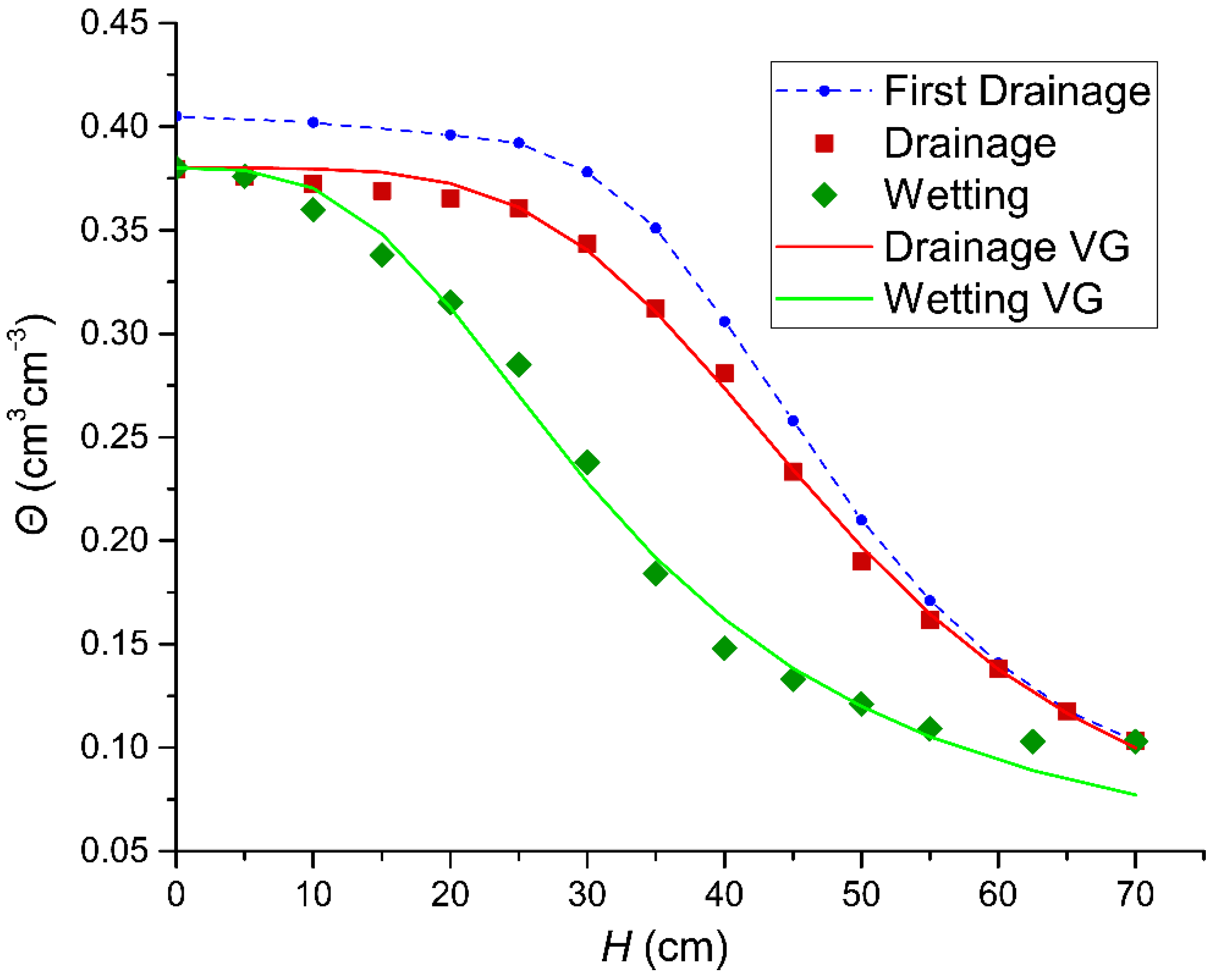
The hydraulic properties of the studied porous material were experimentally determined as follows. Specifically, the Richards’ pressure cell chamber was used for the determination of the boundary wetting and drying curves of the hysteretic loop [25]. The experimental data for the two boundary curves are presented in Figure 1. The saturated hydraulic conductivity, Κs (LT−1), was independently determined by the constant-head method [26].
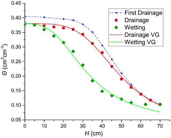
Figure 1.
The experimental data for the boundary wetting and drying curves of the hysteretic loop (points) and the fitted curves according to the Mualem–van-Genuchten model (VG). The corresponding values of parameters of the Mualem–van-Genuchten model are presented in Table 1.
Then, the RETC program [27] was used to calculate the fitting parameters of the widespread Mualem–van-Genuchten model [28,29,30]:
where α, n, and m are fitting parameters; θs is the volumetric soil water content at saturation; θr is the residual volumetric soil water content; m = 1−(1/n); and Se = (θ−θr)/(θs−θr) (degree of saturation or effective saturation).
The parameters were estimated based on the experimental data of soil water content boundary retention curves and saturated hydraulic conductivity (Ks). The unknown parameters of the Mualem–van-Genuchten (M–vG) model in the parameter optimization process to fit the water retention and saturated hydraulic conductivity functions were θr, α, and n. The values of the parameters m and p were taken as m = 1−(1/n) and p = 0.5, a value widely used [28]. The fitted curves of the Mualem–van-Genuchten model to the experimental data are also presented in Figure 1.
2.4. Hydrus 1-D
The HYDRUS-1D software package [21] was used to simulate the infiltration and the subsequent horizontal redistribution in this study. HYDRUS-1D uses the finite element method to solve the Richards’ equation for water flow in an unsaturated porous medium. For one-dimensional horizontal flow, the Richards equation reduces to the following as the influence of gravity is absent:
where θ is the soil water content, H is the soil water pressure, K is the unsaturated hydraulic conductivity (assumed to be a function of the pressure head or equivalently of θ), t is time, and x is the spatial coordinate. Input functions to the HYDRUS-1D code were θ(H) according to the van Genuchten (Equation (11)) [29] analytical expression and K(θ) or K(Se(θ)) (Equation (12)) [28]. The fitting parameters α, n, and θr were obtained from experimental data using the RETC program (Table 1) as described above.

Table 1.
The values of the parameters of the Mualem–van-Genuchten model obtained according to a curve-fitting procedure (RETC program) on experimental measurements and the measured Κs.
When using HYDRUS-1D, every numerical node in the discretized domain can be assigned its own cluster of hysteresis scanning curves depending upon whether wetting or drainage occurs. In our study, we used the approach of Lenhard et al. [12] to generate the various scanning curves. Their method assumes closure of the scanning loops by forcing the scanning curves to pass through the latest wetting or drainage reversal points, thus avoiding so-called artificial pumping errors. In this approach, all scanning curves are scaled from the boundary wetting or drainage curves using the same values of a and n as the boundary wetting or drainage curves.
For the HYDRUS-1D simulations, a horizontal soil column with adequate length (200 cm) and a grid size of 0.5 cm was used based on mesh independence tests. The boundary condition at one side was set to “variable pressure head/flux” to allow the simulation of an initial infiltration for a set time. This condition allowed us to change the boundary condition from the variable pressure head (0 cm) during the infiltration to the variable flux (no-flow) during the redistribution. The boundary condition at the other side was set to “no-flow” as the soil column was long enough, and the water front remained far from this boundary in all cases.
Specifically, from Darcy’s law and the mass conservation principle, the differential equation for the original horizontal infiltration was, as given above in Equation (13), with the initial and boundary conditions given below:
t = 0, θ = θ0, x > 0
x = 0, θ = θs (saturation, as H = 0)
Now, as for the redistribution process, which follows immediately after the cessation of the infiltration at time t = T (duration of infiltration) and which is denoted by τ(T) = 0, the initial condition of the redistribution process is:
τ(T) = 0, θ = θ(x,T), x > 0
Again, the classical Richards’ equation (as given from Equation (13)) applies, and the process of redistribution takes place, either with hysteresis being included, denoted as (HY), or without hysteresis, denoted as (WH). Evaporation was assumed as non-existent in all cases.
3. Results
3.1. Comparison of the Redistribution Profiles with and without Hysteresis When the Initial Water Content Lies on the Boundary Wetting or the Boundary Drying Curve
As the first step, the redistribution profiles with (HY) and without (WH) hysteresis were examined for the case with the initial water content before the initiation where the horizontal infiltration lies on the boundary wetting curve.
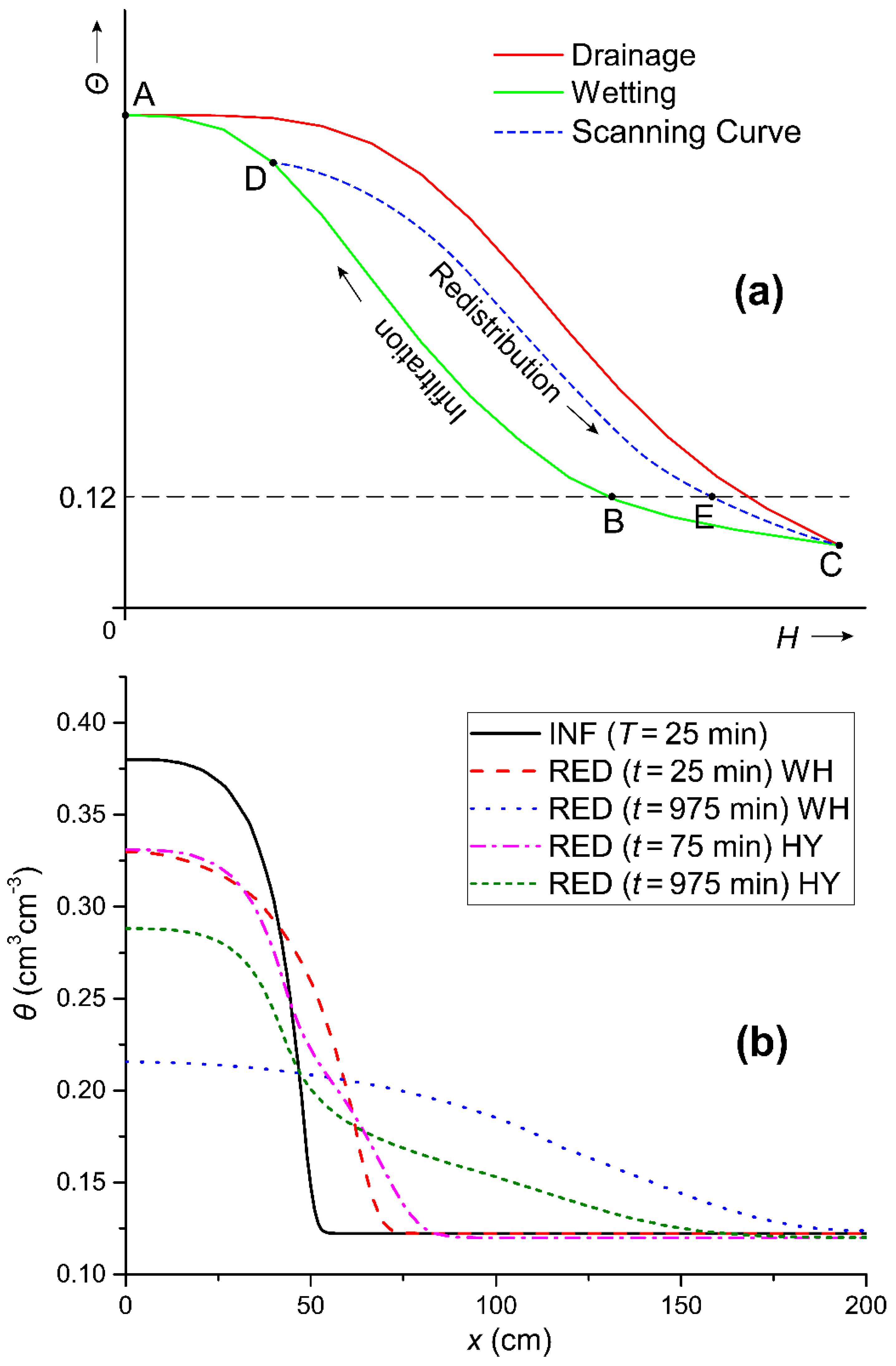
The initial water content chosen was θ0 = 0.12 cm3cm−3 (H = −49.9 cm), the infiltration duration was T = 25 min, and the infiltration depth was 10.863 cm in both cases. The H–θ relationship (for both cases) during the infiltration from the state B caused an increase in θ and H following the boundary wetting curve (Figure 2a). During the redistribution process for the WH case, again, the H–θ relationship in every position in the soil column was following the boundary wetting curve, while, for the HY in every position in the soil column, the H–θ relationship would follow, depending on the θ value attained in the specific soil position, an appropriate drying scanning curve (e.g., DE drying scanning curve, Figure 2a), or the boundary drying curve as such.
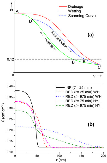
Figure 2.
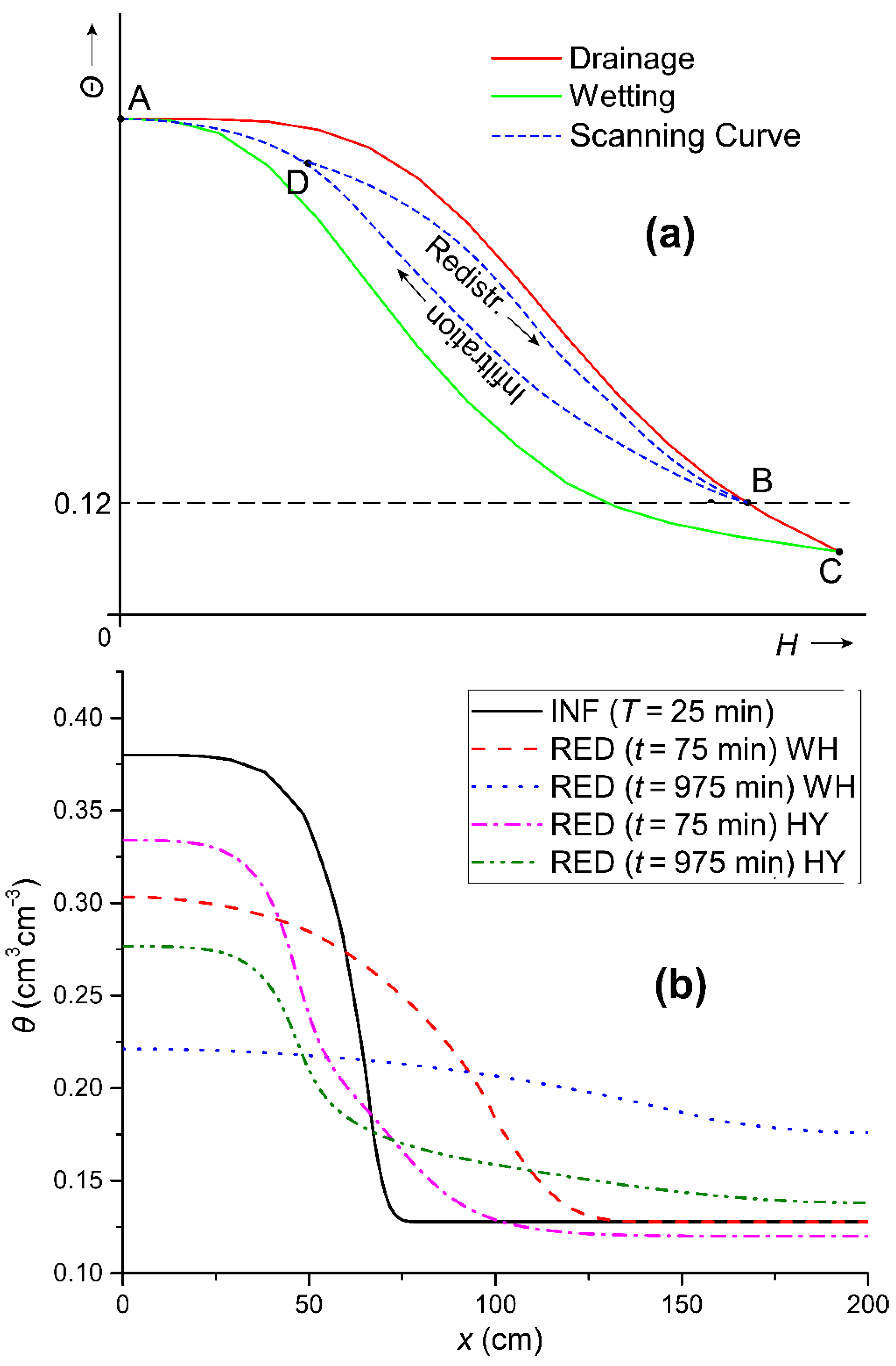
Schematic representation of the boundary drainage and wetting curves and the pathways followed during infiltration and redistribution in the case where the initial water content lies on the boundary wetting curve (a). The θ(x) relationship for the horizontal infiltration (INF) with initial soil water content θ0 = 0.12 cm3cm−3 and for T = 25 min and for the redistribution (RED) when hysteresis was considered (HY) and without hysteresis (WH), making use of the boundary wetting H–θ curve for redistribution times: 25 min (WH) and 75 min (HY) and 975 min for (WH) and (HY) (b).
From Figure 2b, it appears that the process of redistribution (θ-(x,t)) at the early times was faster than later on, for both cases. The phenomenon was more acute for the HY case, where, at the soil surface, the water content at t = 25 min fell to a value θ = 0.331 cm3cm−3 from θs = 0.38 cm3cm−3 (data not shown), while, for t = 975 min, it fell to a value of θ = 0.288 cm3cm−3. The HY redistribution soil water content profiles after the time t = 75 min almost coincided with the one obtained for WH at an earlier time t = 25 min. This confirms that the inclusion of hysteresis causes a large delay in the redistribution process and consequently to soil water removal from the soil root zone where it was originally (with the initial infiltration) stored. One other observation was that the soil water content at the soil surface at a time t = 975 min was θ = 0.288 cm3cm−3, while in the absence of hysteresis it was 0.215 cm3cm−3.
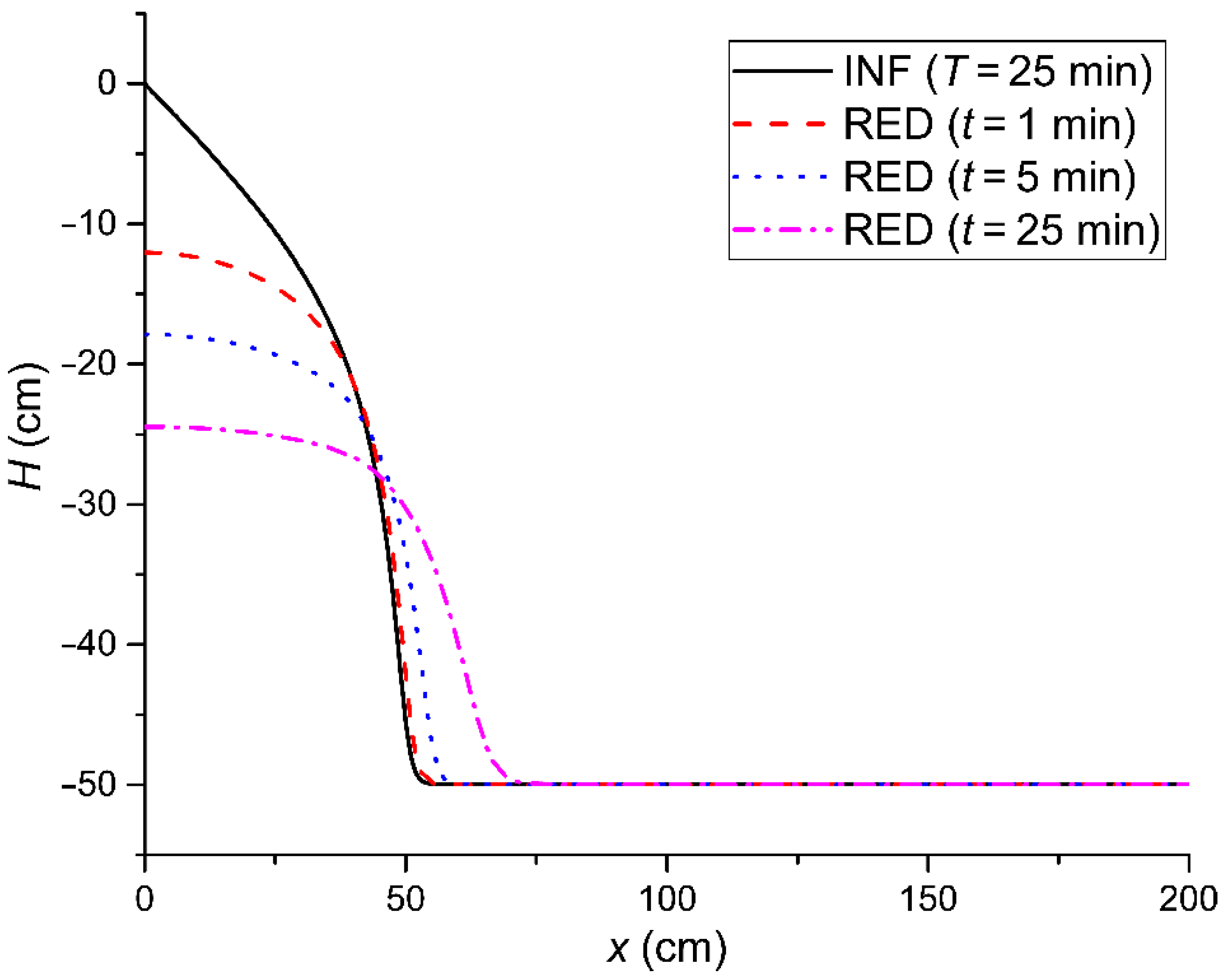
For a better understanding of the effect of hysteresis on soil water redistribution, the pressure head gradient in the pressure head profiles during the redistribution were examined. In Figure 3, it can be observed that the soil water pressure head gradient in the presence of hysteresis at time t = 25 min tended to the value of zero, which explains the small magnitude of the redistribution rate in all later stages—although the values of K and θ were large. The soil water pressure head gradient dH/dx at the same time for the case without hysteresis had greater values, which explains the larger values of the redistribution rate without the inclusion of hysteresis (data not shown).
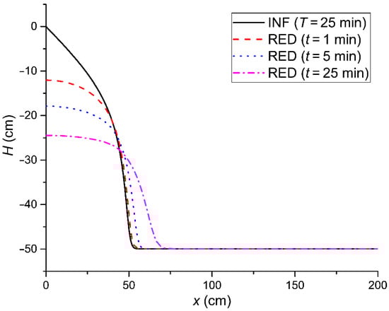
Figure 3.
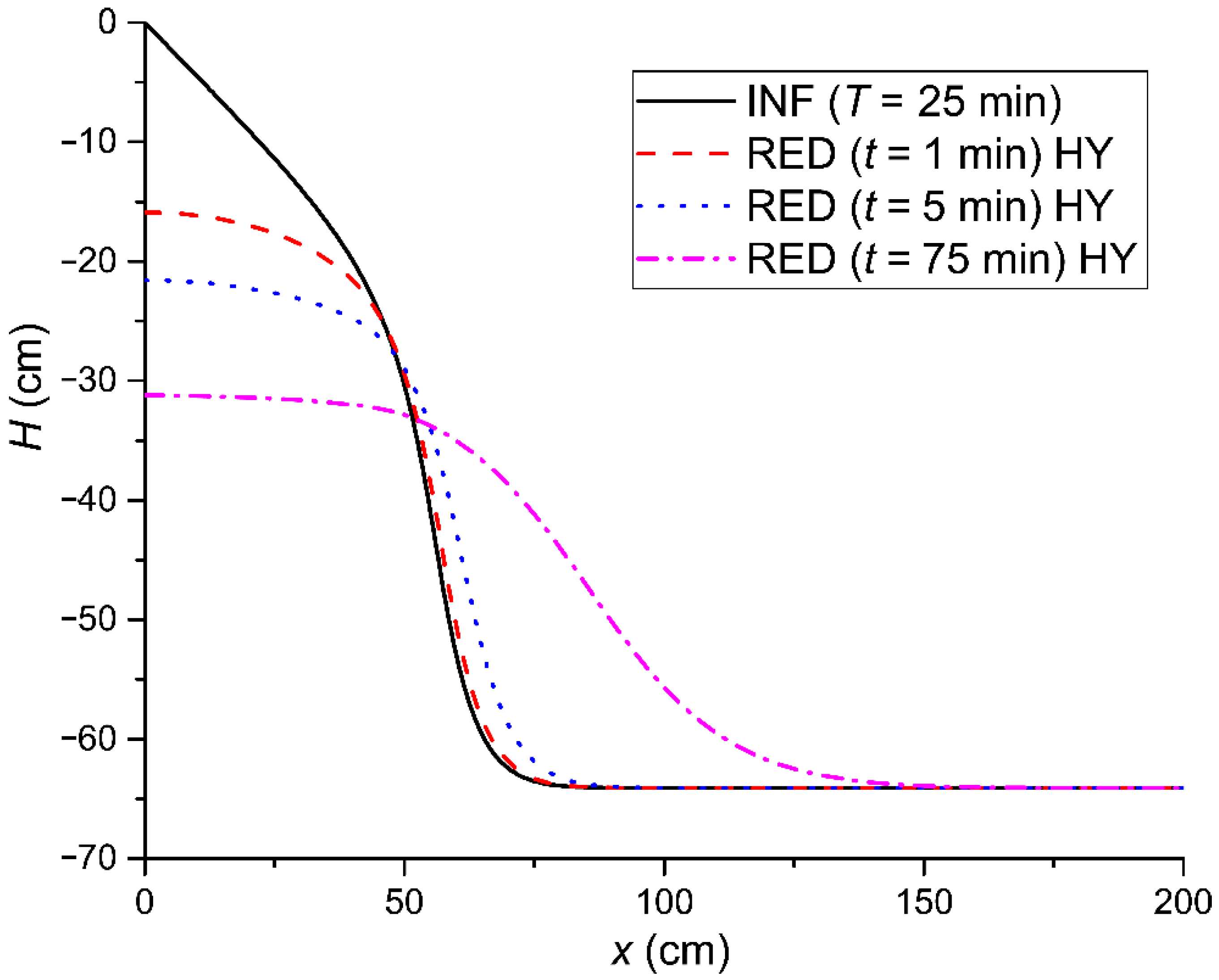
The relation of the soil water pressure head H with the horizontal distance x, H(x), at the end of the horizontal infiltration (INF) with duration T = 25 min and during the redistribution (RED) with hysteresis being included (HY) at times t = 1, 5, and 25 min, after the cessation of the infiltration making use of the boundary wetting H–θ curve. The initial soil water content before the commencement of the infiltration was θ0 = 0.12 cm3cm−3 (H = −49.9 cm).
As the second step, the same comparison was made for the case that the initial water content (θ0 = 0.12 cm3cm−3) before the initiation of the horizontal infiltration lies on the boundary drying curve (state B, Figure 4a). The infiltration depth in this case was I = 12.5 cm for the HY case and I = 15 cm for WH.
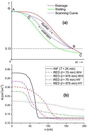
Figure 4.
Schematic representation of the boundary drainage and wetting curves and the pathways followed during infiltration and redistribution in the case that the initial water content lies on the boundary drying curve (a). The θ(x) relation for the case of the initial horizontal infiltration for T = 25 min (INF) with initial soil water content θ0 = 0.12 cm3cm−3 and the case of water content redistribution with the inclusion of hysteresis (HY) and without hysteresis (WH) making use of the boundary drying curve and initial soil water content θ0 = 0.12 cm3cm−3 for two times of redistribution: 75 and 975 min (b).
In this case during infiltration, in all x-positions in the soil column, the soil water content θ and the soil water pressure head H increased from the initial value θ0 = 0.12 cm3cm−3 at H = −64.1 cm lying on the boundary drying curve (state B, Figure 4a), following a first-order wetting scanning curve BDA (Figure 4a). When hysteresis was not considered, the θ–H relation was single-valued and followed the boundary drying curve. In HY, during the redistribution process in the soil zone, where soil water content reduction starts after the cessation of infiltration (the one closer to the soil surface, which is wetter than the rest), the θ–H relation in every position x will follow either the respective 2nd order drying scanning curve DB (Figure 4a) or the boundary drying curve depending on the values of θ and H attained during the original infiltration. From Figure 4b, one may observe that redistribution at early times, after the cessation of infiltration, was faster for both cases (HY or WH), and this appeared to be more obvious for the HY case. In this case, at t = 75 min, θ = 0.334 cm3cm−3 from θs = 0.38 cm3cm−3 while, at t = 975 min, θ = 0.276 cm3cm−3, and, for the WH case, θ = 0.221 cm3cm−3. Comparing the above with the case of using the boundary wetting curve, the values of the soil water content at the soil surface appear rather close to the respective values obtained with or without the inclusion of hysteresis. Nonetheless significant differences were observed at the soil at a distance x = 200 cm, where θ for both cases (HY and WH), when it followed the boundary drying curve, was larger than the initial one, θ = 0.12 cm3cm−3. This phenomenon was more pronounced when hysteresis was not included, since, in this distance (x = 200 cm), θ was even larger (θ = 0.176 cm3cm−3). We should mention that for the case of using the boundary wetting curve soil water redistribution profile development was not advanced up to that distance (x = 200 cm) for both cases (HY or WH).
In Figure 5, it is shown that the soil water pressure head gradient tended to zero at t = 75 min, i.e., in a later time compared to the case where the boundary wetting curve was used. Additionally, from the comparison of the redistribution H(x) profiles at the times t = 1 min and t = 5 min for the cases of the two boundary hysteresis curves, it appeared that the redistribution rate was larger for the case of the boundary drying curve since the soil water pressure head at the respective times had negative values of a larger magnitude.
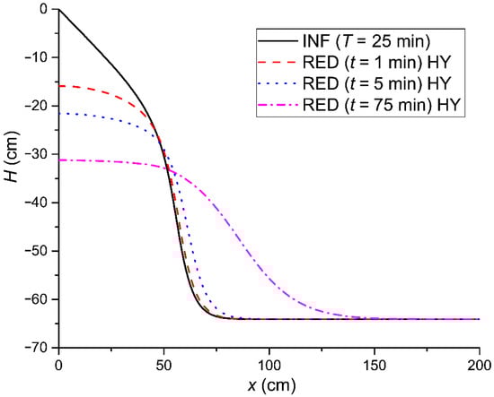
Figure 5.
The relation between soil water pressure head H and horizontal distance x, H(x), after a horizontal infiltration (INF) with duration T = 25 min and during the redistribution (RED) process with the inclusion of hysteresis for time intervals t = 1, 5, and 75 min with initial water content θ0 = 0.12 cm3cm−3 (H = −64.1 cm) and using the boundary drying curve.
3.2. Comparison of the Redistribution Profiles Forms in the Presence of Hysteresis for Different Infiltration Depths and Initial Water Content Values
The redistribution profile forms in the presence of hysteresis for different infiltration depths, I, and initial water content values, θ0, were compared for the case that the initial water content values lie on the boundary wetting soil water content retention curve (Figure 6).
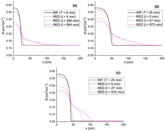
Figure 6.
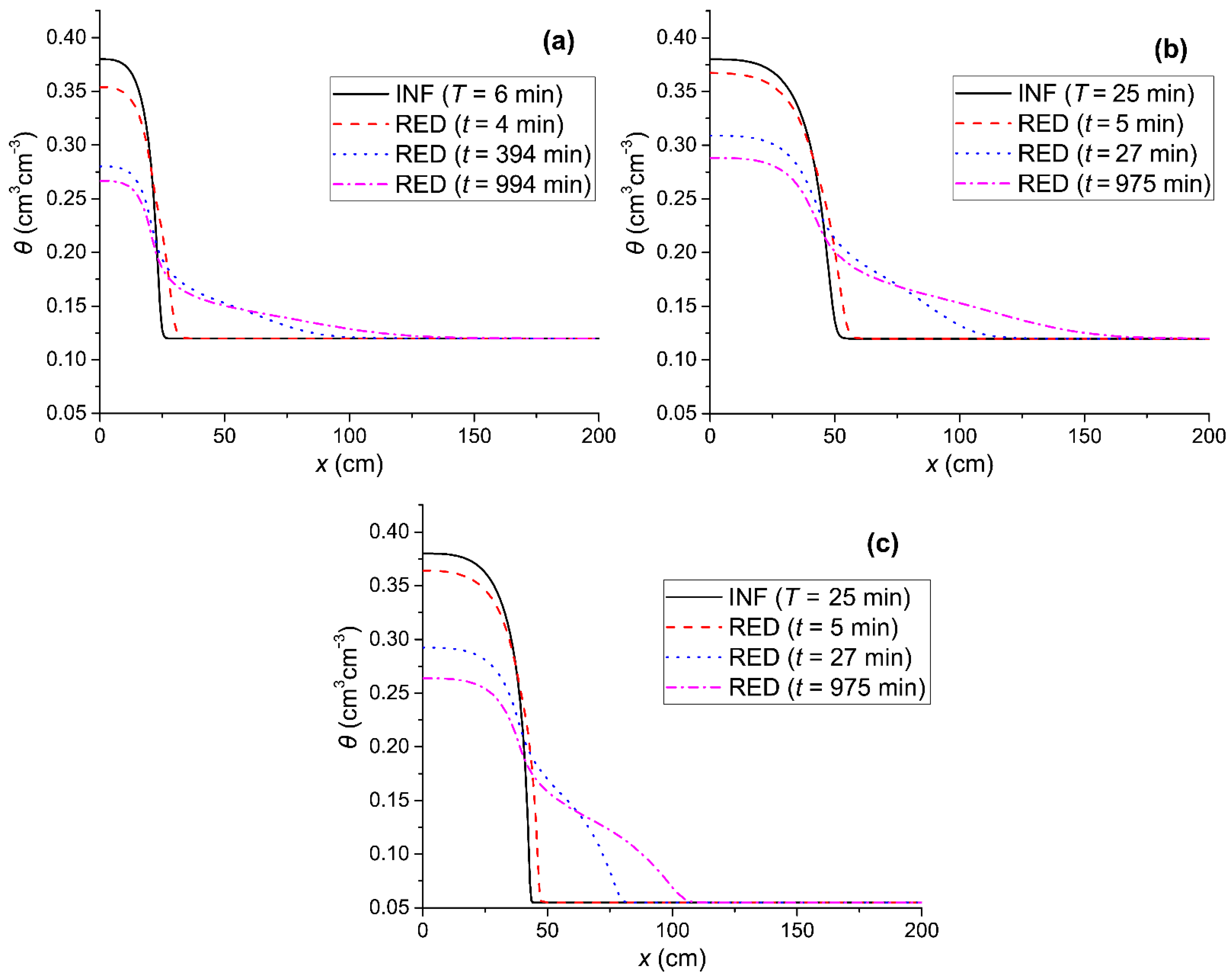
The soil water content profiles of the initial infiltration (INF) and the redistribution (RED) water content profiles for several cases of infiltration water depths, I, and different values of the initial water content. (a) The profiles for θ0 = 0.12 cm3cm−3 and duration of infiltration T = 6 min, corresponding to I = 5.34 cm; (b) the profiles for θ0 = 0.12 cm3cm−3 and duration of infiltration T = 25 min, corresponding to I = 10.9 cm; and (c) the profiles for θ0 = 0.055 cm3cm−3 and duration of infiltration T = 25 min, corresponding to I = 12.3 cm.
From Figure 6, one may observe that in all three cases the redistribution soil water content profiles developed at various times of redistribution, more or less with a similar form as to the original shape of infiltration, with the water content being reduced as the redistribution time increased. The dθ/dx slope during redistribution was negative and approached zero in relatively short times. At the soil surface, one can observe the maximum value of θ, as this is dictated by Equations (5) and (6) in the absence of evaporation. In this respect, the redistribution water content profiles, calculated through the application of the HYDRUS-1D numerical software, for the horizontal infiltration–redistribution case, were compatible with the classical theory of hysteretic soil water movement, which predicts water content profiles of specific forms during the redistribution after infiltration, in comparison to the case of the vertical infiltration–redistribution, where two different forms of moisture-profile development during the redistribution of soil water after infiltration were observed.
3.3. Investigation of the Redistribution Rates for Substantially Different Infiltration Durations and Depths
The redistribution rates were investigated for substantially different infiltration durations and infiltration depths (Τ = 6 min and I = 5.34 cm and Τ = 25 min and I = 10.90 cm), while the values of the initial water content at the commencement of the original infiltration were the same (θ0 = 0.12 cm3cm−3). In this case, we examined, as sub-cases, the ones with small and large time durations of redistribution.
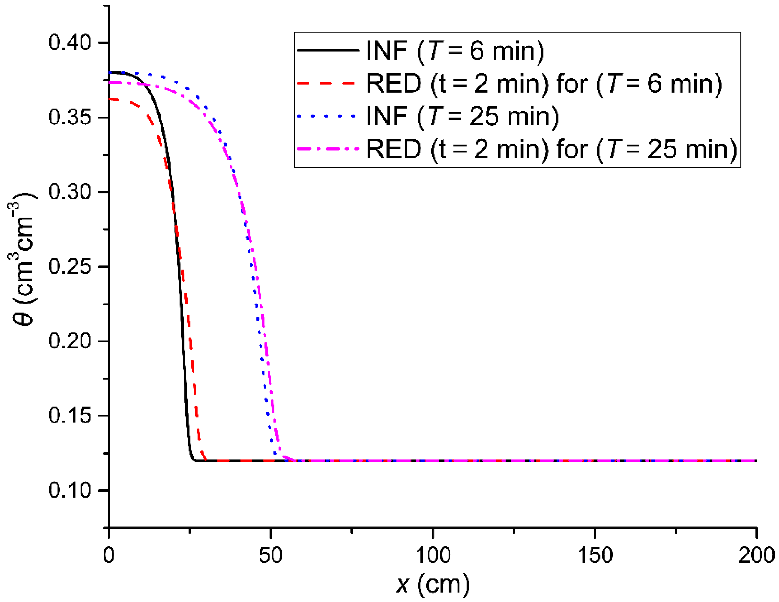
In Figure 7, one may observe that at the same time of redistribution (t = 2 min) the soil water content reduction at the soil surface was larger for the case of the initial infiltration depth I = 5.34 cm compared to that of I = 10.90 cm. In this respect, one could argue that the redistribution rate was larger for the case of a smaller amount of soil water that was initially infiltrated than that of a larger one. More specifically, the value of θ at the soil surface during the redistribution process for the case of a smaller infiltration soil water depth was 0.362 cm3cm−3, while, for the case of the larger original infiltration depth, it was 0.373 cm3cm−3. For the case of the larger infiltration depth, the slope near the soil surface will have a smaller magnitude, and it will tend to zero as the initial infiltration depth increases compared to the respective slope, which will be attained in the case of a smaller depth being originally infiltrated, always assuming that the above refers to the same porous medium and the same initial soil water content before the initiation of the original infiltration process. From the above one could argue that the redistribution rate will be larger in the second case due to the larger magnitude of the soil water pressure head gradient (Equation (3)), and therefore the reduction of the soil surface water content will be larger too.
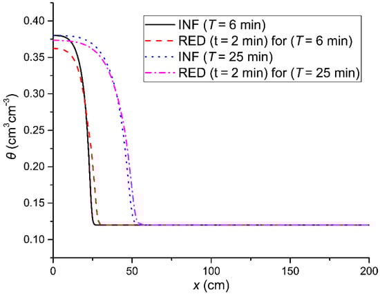
Figure 7.
The water content profiles of the initial infiltration (INF) for two different infiltration durations (T = 6 min and T = 25 min corresponding to I = 5.34 cm and I = 10.90 cm) and for water content redistribution (RED) for small times (t = 2min).
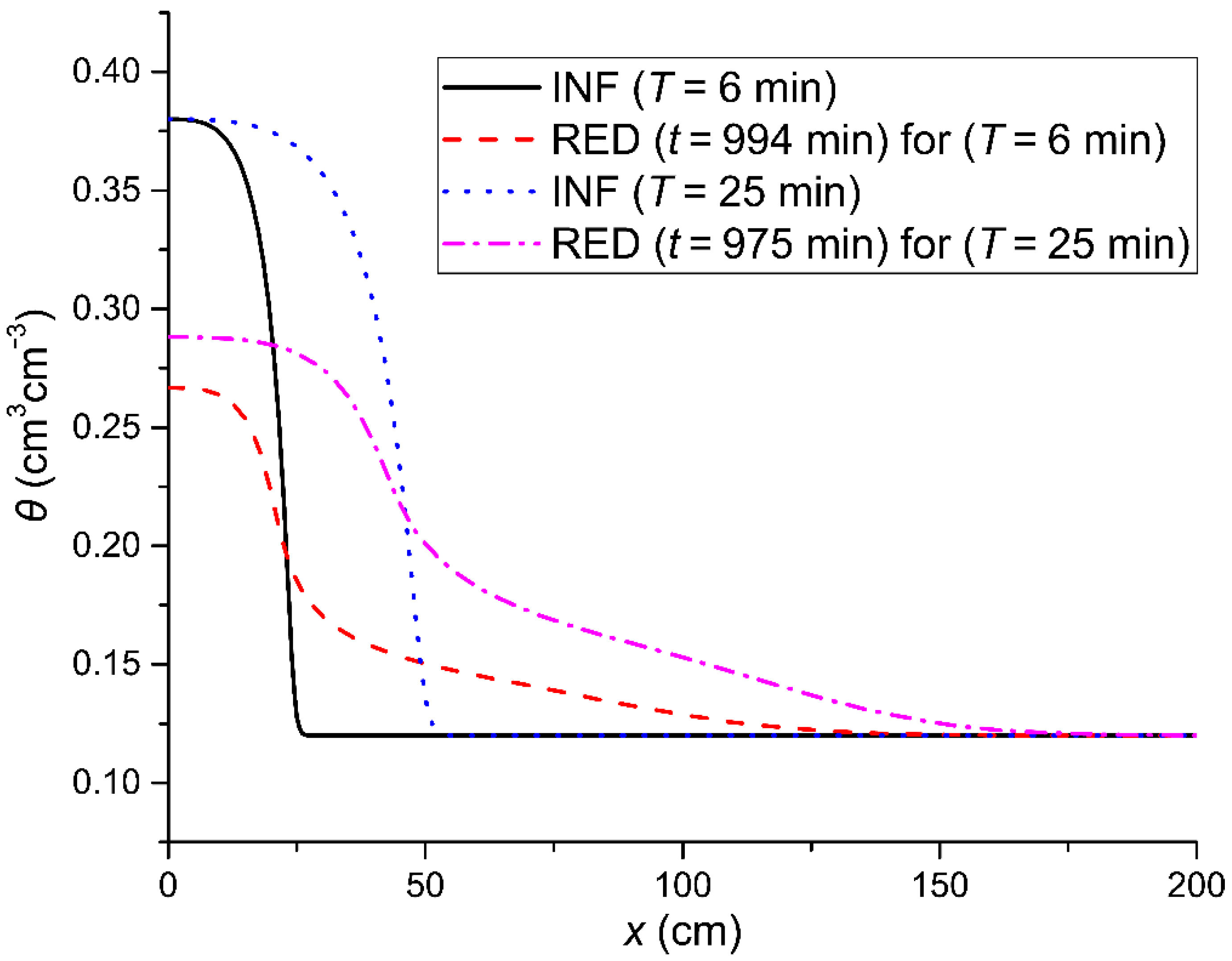
For large redistribution times, i.e., t = 975min, the redistribution rate becomes smaller compared to the early times in the redistribution process. In general, the rate gradually becomes very small for both cases, the soil water content profiles stabilize, and the soil water contents at the soil surface approach a constant value being equal to 0.288 cm3cm−3 (from 0.373 cm3cm−3 at the beginning of redistribution) for the larger infiltration depth and equal to 0.266 cm3cm−3 (from 0.362 cm3cm−3) for the lower infiltration depth (Figure 8).

Figure 8.
The soil water content profiles after the initial horizontal infiltration (INF) for two infiltration durations (T = 6 min and T = 25 min corresponding to I = 5.34 cm and I = 10.90 cm) and their subsequent profiles of redistribution (RED) for large time durations, t = 994 min (for I = 5.34 cm) and t = 975 min (for I = 10.90 cm).
3.4. Comparison of the Redistribution Rates for the Cases That Initial Water Content Values Lie on the Boundary Drying and the Boundary Wetting Curves
The redistribution rates were compared for the case that the initial water content before the original horizontal infiltration was the same (θ0 = 0.12 cm3cm−3) but where it was taken lying on the boundary drying and the boundary wetting curves, respectively.
For this case, if the initial water content θ0 lies on the boundary drying curve then, during the infiltration process, θ and H will increase following the appropriate scanning wetting curve, starting at θ0, while the drying process during redistribution in every soil position will result in reduction in θ and H following the appropriate second-order drying–scanning curve each time. The larger the θ0 value the narrower is the width of the hysteresis loop, which participates during the infiltration–redistribution process.
If the initial water content lies on the boundary wetting curve then, during the original infiltration (wetting), θ and H will increase along the boundary wetting curve, while, at every soil position during drying at the redistribution process, the decrease in θ and H will take place along the appropriate first-order drying–scanning curve.
Poulovassilis [7], studying the respective case for the vertical infiltration–redistribution, gave evidence that the redistribution rate, when the initial water content lies on the boundary drying curve, is larger than for the case when it lies on the boundary wetting curve. The proof was based on the fact that the width of the hysteretic loop, encountered on the vertical infiltration–redistribution process, when the initial value of θ lies on the boundary drying curve, becomes narrower as the initial water content becomes larger. Therefore, ; i.e., the term takes negative values of less magnitude, which are greater when H increases. In this respect, the effect of hysteresis on reducing the magnitude of the soil water pressure head gradient (Equation (3)) becomes lower as the value of the pressure head H at the initial water content θ0 increases, which means that the redistribution rate increases with the increase in the value of the initial water content θ0.
Therefore, it can be expected that when the initial soil water content lies on the boundary drying curve, the redistribution rate will be larger than for the case when the initial water content lies on the boundary wetting curve, considering that the term is the same in both cases.
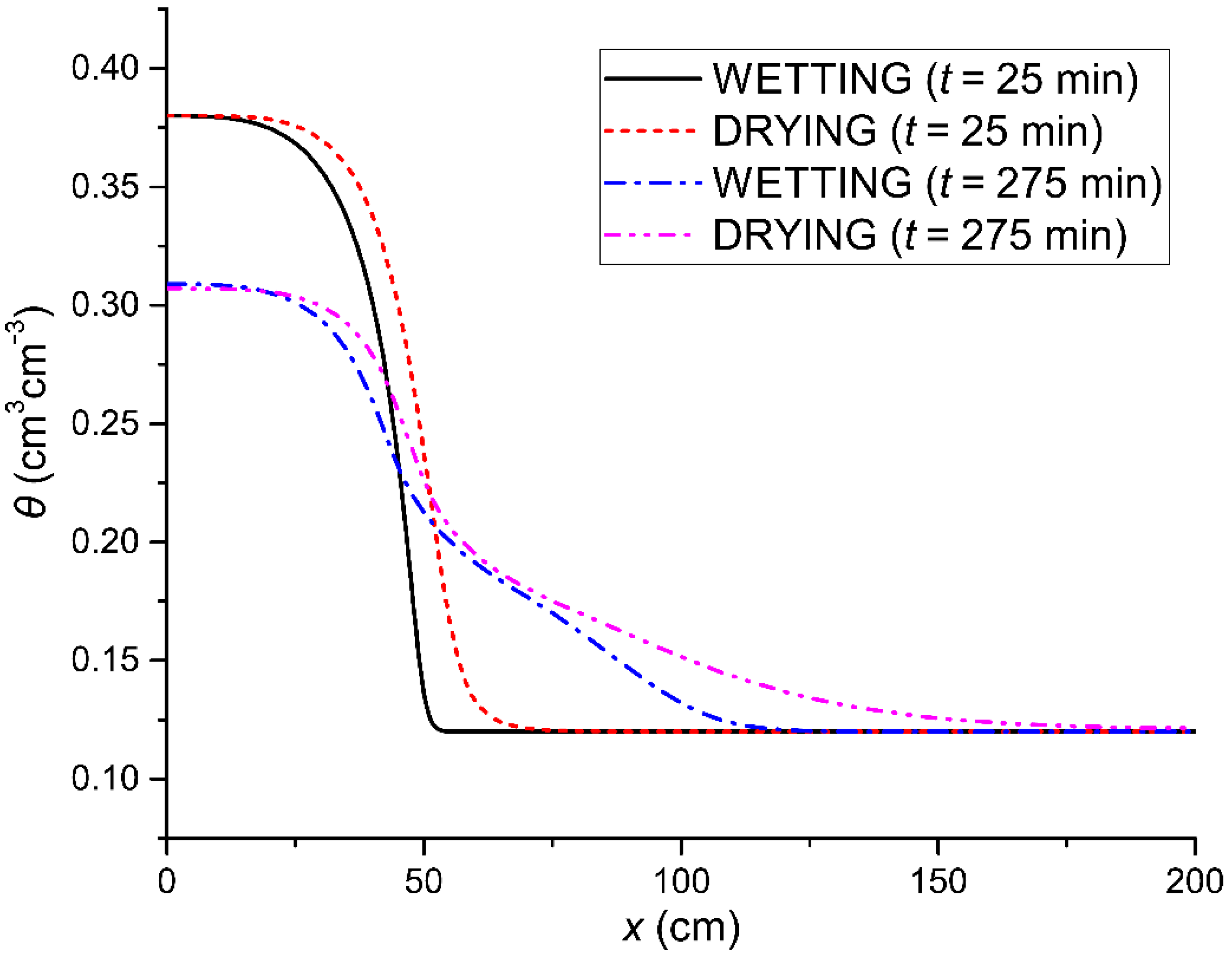
In Figure 9, it is shown that after an original infiltration of T = 25 min duration, the redistribution rate for t = 275 min tended to appear larger for the case where the initial water content lies on the boundary drying curve. In this case, the soil surface water content at t = 275 min was 0.306, while for the case where the initial water content lies on the boundary wetting curve, it was 0.310 cm3cm−3. It could be argued that this small difference can be attributed to the fact that the term was not the same in these two cases, and therefore the effect of the narrower width of the soil water content loop for this occasion was annihilated when the initial water content lies on the boundary drying curve.
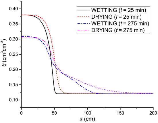
Figure 9.
The horizontal soil water content redistribution (RED) profiles after infiltration with duration (T = 25 min) for times, t = 25 min and t = 275 min, for the boundary wetting (WETTING) and the boundary drying (DRYING) θ–H curves when the initial water content (θ0 = 0.12 cm3cm−3) lies on the respective boundary wetting and drying curves.
3.5. Comparison of the Redistribution Rates for Different Initial Water Content Values Lying on the Boundary Drying and the Boundary Wetting Curves
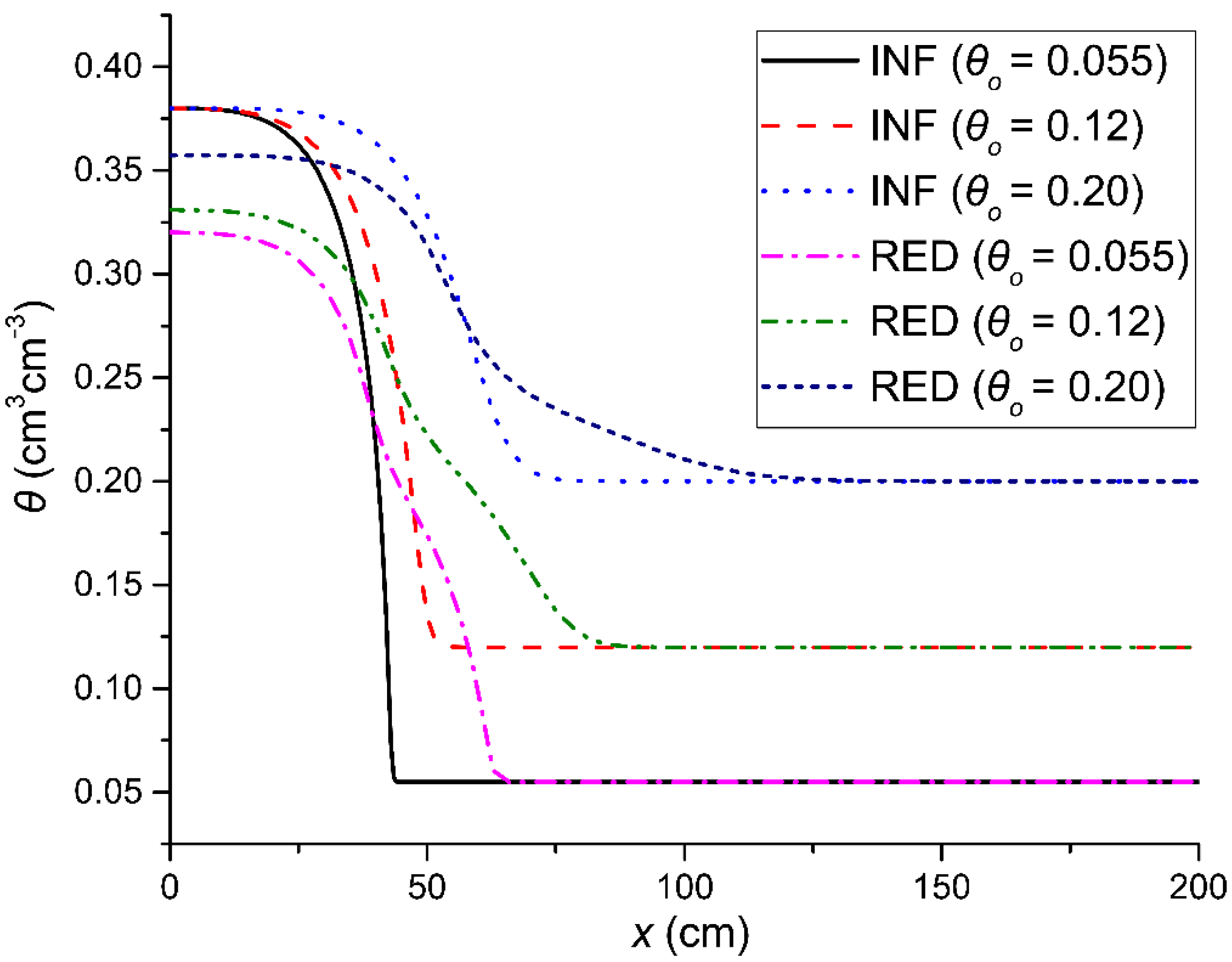
The effect of different values of initial water content before the initiation of the horizontal infiltration (θ0 = 0.055, θ0 = 0.12, and θ0 = 0.2 cm3cm−3) lying on the boundary wetting or boundary drying curve on the redistribution rate was examined when the time duration of the original infiltration was equal to 25 min; it was the same for both cases. The corresponding pressure heads (H) to these initial water content values for the case of the boundary wetting curve were −96.3, −49.9, and −30.3 cm, and for the boundary drying curve, they were −97.2, −64.1, and −49.6 cm.
In Figure 10, the soil water content redistribution profile at t = 75 min is plotted for different values of θ0 lying at the boundary wetting curve. As can be seen in this figure, smaller values of θ0 correspond to a larger redistribution rate. In other words, the redistribution rate was inversely related to θ0 in the case of boundary wetting curves of the hysteresis loop.
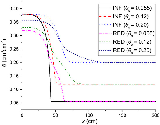
Figure 10.
The soil water content profiles of the initial horizontal infiltration (INF) with duration T = 25 min and of the redistribution (RED) for time t = 75 min after the cessation of the infiltration for different values of initial water content lying at the boundary wetting curve before the commencement of the initial infiltration (θ0 = 0.055, θ0 = 0.12, and θ0 = 0.2 cm3cm−3).
The opposite behavior was observed in the previous section for the cases where the initial water content values varied along the boundary drying curve, in which case larger values of θ0 corresponded to larger redistribution rates.
For the case where the values of the initial water content varied along the boundary wetting curve, an increasing θ0 tended to keep larger values of Hx (Hx being the value of the soil water pressure head at the transition plane separating the drying zone from the wetting one during the redistribution process) and therefore maintained larger values of the pressure head (H) (smaller negative ones) in the drying zone. Therefore, it is anticipated that the redistribution rate decreases with the increase in the values of the initial water content [7].
3.6. General Considerations
Soil water content redistribution is crucial for several hydrologic processes such as infiltration, evaporation, root water uptake, tile drainage, and ground water recharge, including contaminant transport [24]. When soil water content increases or decreases monotonically (e.g., during infiltration, evaporation), the θ(H) relationship can be described by a single retention curve representing either the wetting or the drying cycle. However, because of periodic changes in irrigation flux or the evaporation rate, wetting and drying cycles alternate near the soil surface. Therefore, a single θ(H) curve is not adequate in such cases, and the introduction of hysteresis is required [31].
The obtained results revealed that the redistribution of infiltrated water into the soil was considerably influenced by the presence of hysteresis. A general observation is that the inclusion of hysteresis causes a large delay in the redistribution process and limits horizontal soil water movement after the cessation of the infiltration event. This behavior can be attributed to the effect of hysteresis on the soil water pressure head gradient, which becomes equal to zero soon after the initiation of the redistribution due to hysteresis, as it was also theoretically shown in Section 2.1. This observation may affect the available water in the root zone for the growth of cultivated plants or natural vegetation and should be considered in localized irrigation systems’ design and management. Elmaloglou and Soulis [1] also reported that “draining process progresses more quickly when hysteresis is neglected than when hysteresis is considered” and that “the inclusion of hysteresis results in reduced water losses under the root zone” in the case of drip irrigation. Horizontal redistribution is more important in the case of localized irrigation systems, such as drip irrigation as well as furrow irrigation, where water spreads both vertically and horizontally [1,2]. In these cases though, the investigation of soil water content redistribution is even more complex as vertical and horizontal redistribution occurs at the same time [32].
Furthermore, a better understanding of the redistribution process is important for the efficient management of fertilization as it influences nutrients that move out of the root zone along with water.
4. Conclusions
From the findings of the numerical simulation, applied to the phenomenon of the horizontal soil water infiltration and its subsequent soil water content redistribution, using the HYDRUS-1D software package, it was shown that hysteresis of the soil hydraulic properties, and especially that of the soil water content retention curve, affects seriously the redistribution process, which follows the original horizontal infiltration. The form of the redistributed soil water content profiles in all cases was similar to the shape of the initial infiltration profiles, in comparison to the vertical infiltration–redistribution processes, where two different forms of redistribution profiles were obtained.
The redistribution rate was inversely related to the soil water depth being originally infiltrated and was larger for the early times of the redistribution process, while diminishing substantially and tending to zero for larger time durations due to the reduction in the magnitude of the soil water pressure head gradient in the presence of hysteresis. Thus, while the magnitudes of θ and K could be large enough, nonetheless, soil water movement might be hindered due to the phenomenon of hysteresis. These findings are in accordance with the classical hysteretical soil water theory.
The hysteretical expression of the soil water pressure head gradient constitutes the basis upon which the understanding and analysis of the phenomena associated with the horizontal infiltration–redistribution processes are explained. In every particular problem related to the horizontal infiltration–redistribution process, one should consult the particular expression of the soil water pressure head gradient in an attempt to reach a clear understanding of what is happening.
For a safe evaluation of the HYDRUS-1D software and its embedded model of predicting various, but necessary, hysteretical paths concerning the rather complex phenomenon of horizontal infiltration–redistribution processes, it is necessary to have reliable experimental data and to then carefully attempt the comparison with the numerical ones. This could be the next step of the present work.
Author Contributions
Conceptualization, G.K.; methodology, G.K. and K.X.S.; software, K.X.S.; validation, G.K., K.X.S., and P.K.; formal analysis, G.K.; investigation, G.K.; resources, G.K. and K.X.S.; data curation, G.K. and K.X.S.; writing—original draft preparation, G.K., K.X.S., and P.K.; writing—review and editing, G.K., K.X.S., and P.K.; visualization, G.K. and K.X.S.; supervision, G.K. All authors have read and agreed to the published version of the manuscript.
Funding
This research received no external funding.
Institutional Review Board Statement
Not applicable.
Informed Consent Statement
Not applicable.
Data Availability Statement
Data are available through communication with the authors.
Conflicts of Interest
The authors declare no conflict of interest.
References
- Elmaloglou, S.; Soulis, K.X. The effect of hysteresis on soil water dynamics during surface trickle irrigation in layered soils. Glob. Nest J. 2013, 15, 351–365. [Google Scholar]
- Soulis, K.; Elmaloglou, S. Optimum soil water content sensors placement in drip irrigation scheduling systems: Concept of time stable representative positions. J. Irrig. Drain. Eng. 2016, 142, 04016054. [Google Scholar] [CrossRef]
- Philip, J.R. Horizontal redistribution with capillary hysteresis. Water Resour. Res. 1991, 27, 1459–1469. [Google Scholar] [CrossRef]
- Youngs, E.G. Redistribution of moisture in porous materials after infiltration. Soil Sci. 1958, 86, 117–125. [Google Scholar] [CrossRef]
- Youngs, E.G.; Poulovassilis, A. The different forms of moisture profile development during the redistribution of soil water after infiltration. Water Resour. Res. 1976, 12, 1007–1012. [Google Scholar] [CrossRef]
- Youngs, E.G. The use of similar media theory in the consideration of soil-water redistribution in infiltrated soils. In Advances in Infiltration; ASAE Publication 1183; American Society of Agricultural Engineers: St. Joseph, MI, USA, 1983; pp. 48–54. [Google Scholar]
- Poulovassilis, A. The influence of the initial water content on the redistribution of soil water after infiltration. Soil Sci. 1983, 135, 275–281. [Google Scholar] [CrossRef]
- Heinen, M.; Raats, P.A.C. Unconventional flow of water from dry to wet caused by hysteresis: A numerical experiment. Water Resour. Res. 1999, 35, 2587–2590. [Google Scholar] [CrossRef]
- Mualem, Y. A conceptual model of hysteresis. Water Resour. Res. 1974, 10, 514–520. [Google Scholar] [CrossRef]
- Youngs, E.G. Comments on “Exact Solution for Horizontal Redistribution by General Similarity”. Soil Sci. Soc. Am. J. 2001, 65, 960–961. [Google Scholar] [CrossRef]
- Zhuang, L.; Hassanizadeh, S.M.; Van Genuchten, M.T.; Leijnse, A.; Raoof, A.; Qin, C. Modeling of Horizontal Water Redistribution in an Unsaturated Soil. Vadose Zone J. 2016, 15. [Google Scholar] [CrossRef]
- Lenhard, R.J.; Parker, J.C.; Kaluarachchi, J.J. Comparing simulated and experimental hysteretic two-phase transient fluid flow phenomena. Water Resour. Res. 1991, 27, 2113–2124. [Google Scholar] [CrossRef]
- Poulovassilis, A. Hysteresis of pore water, an application of the concept of independent domains. Soil Sci. 1962, 93, 405–412. [Google Scholar] [CrossRef]
- Poulovassilis, A.; Childs, E.C. The hysteresis of pore water: The non-independence of domains. Soil Sci. 1971, 112, 301–312. [Google Scholar] [CrossRef]
- Poulovassilis, A.; Kargas, G. A Note on calculating hysteretic behavior. Soil Sci. Soc. Am. J. 2000, 64, 1947–1950. [Google Scholar] [CrossRef]
- Philip, J.R. Similarity hypothesis for capillary hysteresis in porous materials. J. Geophys. Res. Space Phys. 1964, 69, 1553–1562. [Google Scholar] [CrossRef]
- Mualem, Y. Modified approach to capillary hysteresis based on a similarity hypothesis. Water Resour. Res. 1973, 9, 1324–1331. [Google Scholar] [CrossRef]
- Jaynes, D. Comparison of soil-water hysteresis models. J. Hydrol. 1984, 75, 287–299. [Google Scholar] [CrossRef]
- Pham, H.Q.; Fredlund, D.G.; Barbour, S.L. A study of hysteresis models for soil-water characteristic curves. Can. Geotech. J. 2005, 42, 1548–1568. [Google Scholar] [CrossRef]
- Hannes, M.; Wollschläger, U.; Wöhling, T.; Vogel, H.-J. Revisiting hydraulic hysteresis based on long-term monitoring of hydraulic states in lysimeters. Water Resour. Res. 2016, 52, 3847–3865. [Google Scholar] [CrossRef] [Green Version]
- Šimůnek, J.; Šejna, M.; Saito, H.; Sakai, M.; van Genuchten, M.T. The HYDRUS-1D Software Package for Simulating the One-Dimensional Movement of Water, Heat, and Multiple Solutes in Variably-Saturated Media; University of California-Riverside Research Reports 3: Los Angeles, CA, USA, 2009; pp. 1–240. [Google Scholar]
- Kool, J.B.; Parker, J.C. Development and evaluation of closed-form expressions for hysteretic soil hydraulic properties. Water Resour. Res. 1987, 23, 105–114. [Google Scholar] [CrossRef]
- Childs, E.C. The ultimate moisture profile during infiltration in a uniform soil. Soil Sci. 1964, 97, 173–178. [Google Scholar] [CrossRef]
- Zhuang, L.; Hassanizadeh, S.M.; Kleingeld, P.J.; Van Genuchten, M. Revisiting the horizontal redistribution of water in soils: Experiments and numerical modeling. Water Resour. Res. 2017, 53, 7576–7589. [Google Scholar] [CrossRef] [Green Version]
- Kargas, G.; Londra, P.A. Effect of tillage practices on the hydraulic properties of a loamy soil. Desalination Water Treat. 2014, 54, 2138–2146. [Google Scholar] [CrossRef]
- Klute, A.; Dirksen, C. Hydraulic conductivity and diffusivity: Laboratory methods. In SSSA Book Series; Soil Science Society of America and American Society of Agronomy: Madison, WI, USA, 2018; pp. 687–734. [Google Scholar]
- Yates, S.R.; Van Genuchten, M.T.; Warrick, A.W.; Leij, F.J. Analysis of measured, predicted, and estimated hydraulic conductivity using the RETC computer program. Soil Sci. Soc. Am. J. 1992, 56, 347–354. [Google Scholar] [CrossRef]
- Mualem, Y. A new model for predicting the hydraulic conductivity of unsaturated porous media. Water Resour. Res. 1976, 12, 513–522. [Google Scholar] [CrossRef] [Green Version]
- van Genuchten, M.T. A Closed-form equation for predicting the hydraulic conductivity of unsaturated soils. Soil Sci. Soc. Am. J. 1980, 44, 892–898. [Google Scholar] [CrossRef] [Green Version]
- Londra, P.; Kargas, G. Evaluation of hydrodynamic characteristics of porous media from one-step outflow experiments using RETC code. J. Hydroinf. 2018, 20, 699–707. [Google Scholar] [CrossRef] [Green Version]
- Russo, D.; Jury, W.A.; Butters, G.L. Numerical analysis of solute transport during transient irrigation: 1. The effect of hysteresis and profile heterogeneity. Water Resour. Res. 1989, 25, 2109–2118. [Google Scholar] [CrossRef]
- Soulis, K.X.; Elmaloglou, S. Optimum soil water content sensors placement for surface drip irrigation scheduling in layered soils. Comput. Electron. Agric. 2018, 152, 1–8. [Google Scholar] [CrossRef]
Publisher’s Note: MDPI stays neutral with regard to jurisdictional claims in published maps and institutional affiliations. |
© 2021 by the authors. Licensee MDPI, Basel, Switzerland. This article is an open access article distributed under the terms and conditions of the Creative Commons Attribution (CC BY) license (https://creativecommons.org/licenses/by/4.0/).