Article

Probabilistic Model for Real-Time Flood Operation of a Dam Based on a Deterministic Optimization Model

by
Víctor Cuevas-Velásquez
1,*,
Alvaro Sordo-Ward
2,
Jaime H. García-Palacios
2,
Paola Bianucci
2 and
Luis Garrote
2
1
Civil Engineering Department, Universidad Andres Bello, Santiago 8370106, Chile
2
Civil Engineering Department: Hydraulics, Energy and Environment, Universidad Politécnica de Madrid, ES28040 Madrid, Spain
*
Author to whom correspondence should be addressed.
Water 2020, 12(11), 3206; https://doi.org/10.3390/w12113206
Submission received: 6 October 2020 / Revised: 5 November 2020 / Accepted: 11 November 2020 / Published: 16 November 2020
(This article belongs to the Special Issue Planning and Management of Hydraulic Infrastructure)

Abstract

:
This paper presents a real-time flood control model for dams with gate-controlled spillways that brings together the advantages of an optimization model based on mixed integer linear programming (MILP) and a case-based learning scheme using Bayesian Networks (BNets). A BNet model was designed to reproduce the causal relationship between inflows, outflows and reservoir storage. The model was trained with synthetic events generated with the use of the MILP model. The BNet model produces a probabilistic description of recommended dam outflows over a time horizon of 1 to 5 h for the Talave reservoir in Spain. The results of implementing the BNet recommendation were compared against the results obtained while applying two conventional models: the MILP model, which assumes full knowledge of the inflow hydrograph, and the Volumetric Evaluation Method (VEM), a method widely used in Spain that works in real-time, but without any knowledge of future inflows. In order to compare the results of the three methods, the global risk index ( I r ) was computed for each method, based on the simulated behavior for an ensemble of hydrograph inflows. The I r values associated to the 2 h-forecast BNet model are lower than those obtained for VEM, which suggests improvement over standard practice. In conclusion, the BNet arises as a suitable and efficient model to support dam operators for the decision making process during flood events.

1. Introduction

Floods can cause enormous economic damage and human suffering, thence, vulnerable areas require control measures to reduce the impacts [1,2]. In regulated basins, reservoirs play an essential role in mitigating the effects of floods [3,4,5,6]. However, the potential conflicts between flood control and the regular operation in multipurpose reservoirs imply a great challenge in the operation decisions [5,7,8,9]. During floods, dam operators often make decisions based on imperfect and incomplete information (for example, data provided by a limited number of sensors) and, in a partial knowledge of the hydrological response of the contributing basin [10]. In addition, there is still huge uncertainty regarding the proper operation of a reservoir for real-time flood control, that increases the risk in the discharge decision-making process [11,12].
The management of reservoirs for flood control in real-time has been historically addressed through curves derived from predefined rules obtained by means of simulation techniques [8], or by using programmed management methods, such as Volumetric Evaluation Method (VEM) [13], widely used in Spain. These methods, reactive in nature, have been included in the reservoir regulation rules and help the operators to manage the dam [6]. Other approaches to real-time flood control in reservoirs are based on risk and uncertainty analysis, leaving decision-makers to choose the model to use according to different emergency scenarios and the initial water level of the reservoir [14], or, in the determination of relationships between double-peak floods, reservoir storage capacity and discharge capacity [15]. Currently, advances in optimization and learning techniques have allowed a new approach to the treatment of the problem of reservoir management in real-time, incorporating the uncertainty caused by the stochastic nature of the inflow hydrographs to the reservoir [16]. There is a wide variety of programs and models regarding the forecast of the inflow hydrographs and the optimization of the dam operation, each with its strengths and weaknesses [17].
The hydrologic dam safety is based on minimizing the risk and consequences of both, the dam infrastructure and downstream discharges [6,18]. In recent decades the use of optimization techniques has attracted the attention of many researchers to develop optimal reservoir operation policies [17,19,20,21] and taking into account different objectives simultaneously [7,12]. These techniques were mainly based on: Linear Programming (LP), Mixed Integer Linear Programming (MILP), Non-Linear Programming (NLP), Successive Linear Programming (SLP), Dynamic Stochastic Programming (SDP), Genetic Algorithms (GA), Genetic Programming (GP), Optimization of Swarm Particle (PSO), Honey-Bee Crossing (HBM), and Artificial Bee Colony (ABC), as well as hybrid models that combine the previous ones. A detailed description of these techniques is presented by Choong and El-Shafie [17]. Among these methods of optimization, the Mixed Integer Linear Programming (MILP) is widely used. It allows to combine real, integer and binary variables [21,22]. The MILP model has the advantage of simplicity and flexibility [23,24], the guarantee that the solution corresponds to the global optimum [12] and its efficiency in solving reservoir optimization problems [24,25,26]. It is fairly easy to adapt the model formulation to different cases by adjusting the model parameters [21,24,27,28], to obtain good results [21,29,30]. However, its main disadvantage is that all relations involved (objective functions and constraints) are required to be linear or linearizable. Although the robustness of MILP models, solving them for very large systems may be computationally more expensive than other optimization models (e.g., NLP).
In most cases, the lack of complete and sufficiently long records of precipitation and gauging increases the uncertainty in the estimation of extreme floods [2,31], which, added to a lack of precise flood forecasting techniques, makes it difficult to determine optimal operation of reservoirs [18,32]. Although reservoir management optimization models allow simultaneous reduction of released flows and appropriate storage allocation during floods, their applicability for real-time management is limited by the forecast accuracy. Indeed, for their correct operation, most of these models are coupled to flood forecasting models in order to increase the known length of the hydrograph entering the reservoir [33,34,35]. If stochastic modeling techniques are additionally considered to quantify the uncertainty about future inputs to the reservoir, the optimization models become excessively complex. This fact limited the practical usefulness of these techniques [36,37]. On the other hand, deterministic optimization models cannot quantify the uncertainty in the parameters of the model or future flows. As an alternative, learning algorithms are characterized by their fundamental ability to deduce behavioral models of a system from measured information, showing in general, good accuracy and a moderate formulation [38].
Bayesian inference stands out among learning techniques. In this approach, uncertainties are expressed in terms of probability distributions [16,36].
Some interesting applications of Bayesian Networks (BNets) include the definition of the optimal shape of double-arch dams, associated with the decrease in the use of concrete [39], the search for the optimal geometric parameters (area and volume) for double-arch dams based on static and dynamic internal stresses [40].
Recent research in the field of hydrology has used BNets to identify the driving factors of flood loss at residential buildings and gaining insight into their relations [41], to develop dynamic predictive models for annual runoff temporal behavior of high dependence rivers [42], to assess temporally conditioned annual runoff fractions in unregulated rivers [43], to quantify the forecast uncertainty by a model for ensemble flood forecasting [2], to perform the dynamic assessment of flood in urban underground spaces [44], to develop a self-adaptive real-time correction model to reduce uncertainties in flood forecasting [45], and to estimate uncertainty in catchment modelling parameter values and uncertainty in design flow estimates [46].
Regarding real-time flood control reservoir operation, BNets have been built as decision support tools, including, for example, the probabilistic modeling of the behavior of a reservoir to control flash floods [36], the development of monthly operating rules for a cascade reservoir system with the objective of controlling floods and supply irrigation needs [47], the analysis of the risk of a single reservoir dam overtopping and two reservoirs collapsing under the combined action of flood and landslide surge [48], the risk analysis for real-time flood control operation of a multi-reservoir system using a dynamic BNet [49] and the risk analysis of reservoir flood control considering the uncertainty of the inflow to a reservoir and the initial level of the reservoir [50].
All these studies have in common the use of Monte Carlo techniques to simulate the hydrological series that are later used for the training of BNets.
On the other hand, the models used to operate the reservoirs include VEM programmed management model [36], models of predefined operating rules specific to each dam [48,49,51] and an optimization model that minimizes the maximum discharge flow [50].
The MILP model may consider, simultaneously, both objectives: dam safety and downstream protection, during each synthetic flood event generated with Monte Carlo techniques.
In this study, a probabilistic real-time reservoir operation model for flood control was developed, which integrates the advantages of a deterministic reservoir optimization model (MILP) and overcomes its limitations derived from the requirement of full knowledge of the inflow hydrograph. The proposed model is built using a case-based learning scheme (BNets) from an ensemble of synthetic events simulated with the MILP model.

2. Materials and Methods

2.1. The Real-Time Reservoir Operation Problem Approach

The real-time flood control optimization approach was addressed by coupling a MILP model with a BNet model. Additionally, an ensemble of synthetic hydrographs for model training was generated.
The applicability of the MILP model for real-time reservoir operation is limited, because it requires full knowledge of the inflow hydrograph. This limitation is overcome by using the output series produced by the MILP model to train a data-based learning model. The model thus built can be used in real-time to produce management recommendations based on the optimizations, but using only the available information. This approach may lead to a more efficient implementation and easier interpretation compared with other real-time operation frameworks. Formulating the real-time model using a BNet scheme was chosen because it can capture the complex causal relationships among variables during training, but its operation is easy and it can assist the decision-maker in the rapid assessment of the situation [36].

2.2. Formulation of a BNet

A BNet is a specific type of graphical model, composed of nodes and directed links, called a directed acyclic graph (DAG) [52]. The nodes represent the model variables and the links the conditional dependency relationships. In general, knowing the values of the nodes X = X 1 , , X n , the joint probability function for any BNet [53] is:
P ( X ) = i = 1 n P ( X i | p a r e n t s ( X i ) ) ,
where, X i is the i t h qualitative value of variable X , P ( X ) is the joint probability of all of the variables, represented by the product of the probabilities of each variable X i given its parent’s value: p a r e n t s ( X i ) . This shows the meaning of the links: they indicate which other variables a given variable is conditioned upon. The links in a BNet are sometimes looked at as causal connections where each parent node causes an effect on its children [53]. For example, if variable F depends on E and variable G depends on E and F, the joint probability would be:
P ( E , F , G ) = P ( E ) × P ( F | E ) × P ( G | E , F ) ,
Inference is the task of computing the probability of each value of a node in a BNet when other values of the variables are known. There are different algorithms for doing inference in a BNet. The learning of a BNet is divided in two types: the learning of the structure and the learning of the parameters (probability distributions). The learning method depends on the knowledge of the structure and the degree of observability of the parameters. The structure can be defined thanks to expert knowledge, but if it is unknown, two tasks must be performed: a metric to compare possible structures and a search algorithm to find potential structures. The cause–effect logical refers to the relationship between the variable represented by parent node (cause) and the variable represented by child node (effect). In the case of parametric learning in a BNet with partial observability, the expectation-maximization (EM) algorithm is used [54].

2.3. Case Study

The proposed methodology was applied to the Talave Dam, located in the Mundo River (southern Spain) and belonging to the Segura River Basin (Figure 1). The mean annual rainfall in the basin is 557 mm and the maximum annual flood was 600 m3/s (year 1996).
Table 1 shows the characteristic levels of the Talave reservoir and the associated volumes.
Analogously, Table 2 presents several characteristic flows related to the downstream river reach capacity.
The Talave dam is equipped with the following outlets:
  • Gated spillway located on the left side, with a threshold level 505.9 m and provided with two bays six meters each. The discharge capacity at DFL (fully open) is 284.9 m3/s.
  • Fixed crest spillway (emergency spillway), located on the right side of dam, being the threshold level 510 m. The length of the spillway crest is 13.5 m and the discharge capacity is 41 m3/s.
  • Bottom outlet with its axe at 475.8 m. The outlet discharge capacity at DFL is 99.55 m3/s.
  • Former intake consists in two conduits at 494.6 m, with a discharge capacity at DFL up to 18 m3/s.
  • Newest intake (also two conduits) at 476.12 m, having a discharge capacity of 123 m3/s at DFL.

2.4. Stochastic Generation of Hydrological Forcing

The Monte Carlo simulation technique was used, which is described below, to generate a large number of synthetic episodes that will serve to train the BNet. The inflow flood events were estimated by applying a semi-distributed event-based hydro-meteorological model that modeled the main physical processes from the rainfall generation to the estimation of the inflow floods [55,56]. In order to obtain a set of stochastic rainfall events, a sample of 1000 uniform distributed values corresponding to the probability of exceedance ( p ) were generated. Being the return period R p = 1 / p , the annual maximum daily precipitation was calculated according to the probability distribution function SQRT-ETmax [55,57,58]. The total precipitated volume ( P t ) for a duration D was estimated by applying the intensity-duration-frequency (IDF) curves proposed by the Ministry of Public Works of Spain [59] and recommended by the Spanish Committee of Large Dams [60]. In order to estimate the temporal distribution of each storm event, it was assumed that the episodes generated were random and not correlated. The temporal distribution of each episode was estimated with an autoregressive moving average model (ARMA(2,2)). The model and its orders ( p and q ) were selected based on an analysis of rainfall data available for Spain (source: Automatic Hydrological Information System; SAIH) and results found in the literature [61,62,63,64].
Many time-series techniques used to model water resources series are based on ARMA linear stochastic processes [62].
A model of this type is denoted by ARMA( p , q ) and, it is composed of two parts: AR( p ) (autoregressive component) and MA( q ) (moving average component), where p and q are parameters that identify the order of each part. The autoregressive part describes the time series of p previous data and the moving average part describes the current and q previous values of white noise.
x t = ϕ 1 × ( x t 1 μ x ) + ϕ 2 × ( x t 2 μ x ) + + ϕ p × ( x t p μ x ) + η t + θ 1 × η t 1 + θ 2 × η t 2 + + θ q × η t q + μ x
where x t is the time series; η t is white noise, i.e., a non-correlated, zero-mean random variable that is also not correlated with the past values of x t ; ϕ 1 ϕ p and θ 1 θ q are the auto-regressive and moving-average parameters, respectively; and μ x is the mean of the time series.
The ARMA(2,2) process was chosen because it has a correlation structure equivalent to the Neyman-Scott rectangular pulses model [62], which has been proved to represent the stochastic structure of rainfall better [65]. Furthermore, the ARMA(2,2) model structure has been used in previous studies to disaggregate daily precipitation, generating synthetic hyetographs, in specific studies of the Segura river basin [21,55,56].
The ARMA(2,2) model parameters were adjusted for 32 rainfall episodes recorded in the basin in the period March 2009 to February 2013, obtaining: ϕ 1 = 0.12, ϕ 2 = 0.16, θ 1 = 0.33, θ 2 = 0.11.
The rainfall-runoff transformation was estimated by applying the curve number method [66]. Subsequently, the hydrographs was generated by applying the dimensionless unit hydrograph method of the Soil Conservation Service [66]. 42% of single peak hydrographs, 48% double peak, 9% triple peak and 1% quadruple peak were generated. Muskingum method was used to estimate the routing of the hydrographs [67]. A detailed description of the methodology to generate the flood events was presented in Sordo-Ward et al. [55,56].
The lower R p events can be regulated in the dam by gate operations, however, for higher R p events the gates become fully opened and the operation rules of the gates decreases in importance for regulation purposes. The Monte Carlo simulation process should generate a sufficient number of cases to cover a wide range of combinations of values that can be expected during the operation of the BNet model [36]. Synthetic episodes were generated for three reasons: (1) to train the BNet, (2) to evaluate the learning process of the BNet and (3) to verify the performance of the BNet. In order to train the BNet 30,000 episodes were generated, to evaluate the learning process 20,000 episodes were generated and, to verify its performance, 2000 episodes were generated. Altogether, 52,000 synthetic episodes were generated.
The number of episodes for the various tasks (training, evaluation, and performance verification) was selected based on the stability of the conditional entropy of the BNet [68].
The conditional entropy quantifies the average degree of dispersion of the variable X when the state of the variable Y is known, and is given by the expression:
H ( X | Y ) = i = 1 m p ( y i ) × [ j = 1 n p ( x j | y i ) × l o g [ p ( x j | y i ) ] ] ,
where H ( X | Y ) is the conditional entropy, X = x 1 , , x n represents the set of values of the child node of the BNet and the variable Y = y 1 , , y m is the set of values of the parent nodes of the BNet.
The 50,000 episodes used to train and evaluate the BNet were plotted to determine the number of episodes for which the conditional entropy stabilizes (Figure 2).
The conditional entropy stabilizes, approximately, at the value 0.125, for the first 30,000 episodes, remaining relatively constant until reaching 50,000 episodes. For this reason, 30,000 episodes were chosen to train the BNet and the remaining 20,000 to evaluate it.
The conditional entropy of the 2000 episodes used in the performance verification is 0.124, very close to the stable value of the conditional entropy for the set of 50,000 episodes. For this reason, 2000 episodes were considered an adequate number to verify the performance of the BNet. Hyetographs of uniformly distributed duration were considered, with values between 10 and 80 h. This range of values is characteristic of the Segura river basin [69]. The Talave reservoir basin was divided into three homogeneous sub-basins. The semi-distributed hydrological model was calibrated based on 32 hourly rainfall events recorded simultaneously in four rain gauges of the Segura basin and Guadalquivir basin and in the azud de Liétor gauging station, located 8.2 km upstream from the Talave reservoir, in the period March-2009 to February-2013. This hydrological model was used to generate the 52,000 hourly flow hydrographs from the 52,000 previously generated synthetic rainfall hyetographs.

2.5. Optimal Reservoir Management

In order to obtain the optimal reservoir response to hydrographs entering the reservoir, the MILP model proposed by Bianucci et al. [21] was used. The main concepts are briefly presented here. This model transforms (as input signal) the input flood hydrograph into two output time series corresponding to the output hydrograph and the evolution of levels in the reservoir.
The MILP optimization model minimizes a cost or penalty function ( P ) subject to operational and hydraulic constraints. The objective function, P , is the weighted sum of two penalty terms (Equation (5)), one corresponding to the reservoir volumes ( P S ) and the other corresponding to the discharged flows ( P O ).
min P = min ( w s × P S + w o × P O ) ,
where w s and w o are the corresponding weights. These penalty terms are related to the dam safety and the downstream safety, respectively.
As mentioned, all the relationships must be linear. Consequently, partial penalty functions ( P S and P O ) and constraints functions were defined as piecewise linear functions and binary variables were included. Complementarily, these functions were parameterized to represent a specific case study. The main advantage of applying the MILP model is that, for each flood, an optimum solution (minimum penalty) is achieved, representing an envelope situation which is not possible to reach using simulation methods based on traditional reactive operation rules (defined by if-then-else statements). Nevertheless, the main drawback of using the MILP model for real-time operation is its dependency on the flood forecast quality as it requires knowing, beforehand, the flood hydrograph for an efficient optimization. Using MILP, the hydrographs of discharged flow and the series of evolution of volumes in the reservoir were obtained, from the 52,000 episodes generated in the previous section. The volume series was transformed into level series using the storage-level curve of the reservoir. For simulation purpose, the initial level was fixed at the maximum normal operation level (TCP), which is the maximum level that is reached during normal operation of the reservoir (before the flood). This assumption is commonly used in dam design [70,71].

2.6. Construction and Evaluation of a BNet

During a flood, the basic variables involved to characterize the routing process in the Talave reservoir are: inflow to the reservoir, reservoir water level, and outflow from the reservoir. The variables were defined considering their possible cause–effect relationships, and adding the time lag factor between them, with expert knowledge (Table 3).
With these variables and their dependency relationships, the BNet structure was built (Figure 3).
Although the structure of the BNet is unique, the child node O t + i is different depending on the forecast time step. For this reason, to refer to a specific forecast interval of the BNet, the notation was used: BNeti, where i can take one or more values from 1 to 5 h. Before training the BNet, the variables (or nodes) were discretized in class intervals within the range of values of the synthetic episodes. Later, the subset of 30,000 synthetic episodes generated according to the procedure indicated in the previous sections was used, to train the BNet, obtaining the Conditional Probability Tables (CPTs) for each node. The trained BNet allow the probabilistic inference of the flow discharged by the reservoir in a forecast time t   +   i , where i varies between 1 and 5 h.
In order to evaluate the learning process of the BNet, the attributes of forecast quality, ability, and precision were estimated, with the subset of 20,000 synthetic episodes generated according to the procedure indicated in the previous sections. Table 4 shows the values of the area under the Relative Operating Characteristic (ROC) curve [72], which quantifies the ability, and the Ranked Probability Score (RPS) index [73], which quantifies the precision.
The area under the ROC curve of the BNet has values close to 1 that decrease slightly as the forecast interval increases. This means that the BNet ability is close to the maximum possible. The RPS index of the BNet has values close to 0, which increase slightly as the forecast time step is greater. This means that the forecast of the BNet is almost perfect with respect to this attribute.

2.7. BNet Application Strategy

Considering that a BNet returns the probability distribution of values over the class interval of the child node, O t + i can take any value within the class interval. A procedure to select a single value of the flow discharged at each instant of time was developed to facilitate the work of the operator of the dam. It was observed that most of the discharge hydrographs resulting from the application of the MILP method have a plateau shape. In the first hours, the flows discharged are very similar to the inflows in the reservoir, therefore, the level of the reservoir remains practically constant. From a certain point, the outflow decreases with respect to the inflow and the level of the reservoir begins to rise.
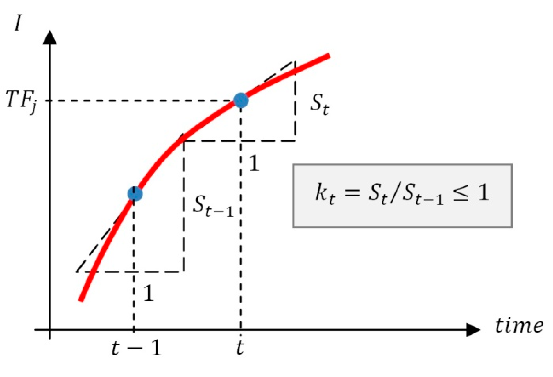
This point, located in the ascending branch of the input hydrograph, corresponds to the instant in which the slope ratio between two consecutive time intervals ( k t = S t / S t 1 ) takes a value less or equal than 1, where S t is the slope of the input hydrograph at time t . This threshold flow must be identified ( T F j ) in all the ascending branches of the input hydrograph, where subscript j represents the last ascending branch up to the current moment (Figure 4).
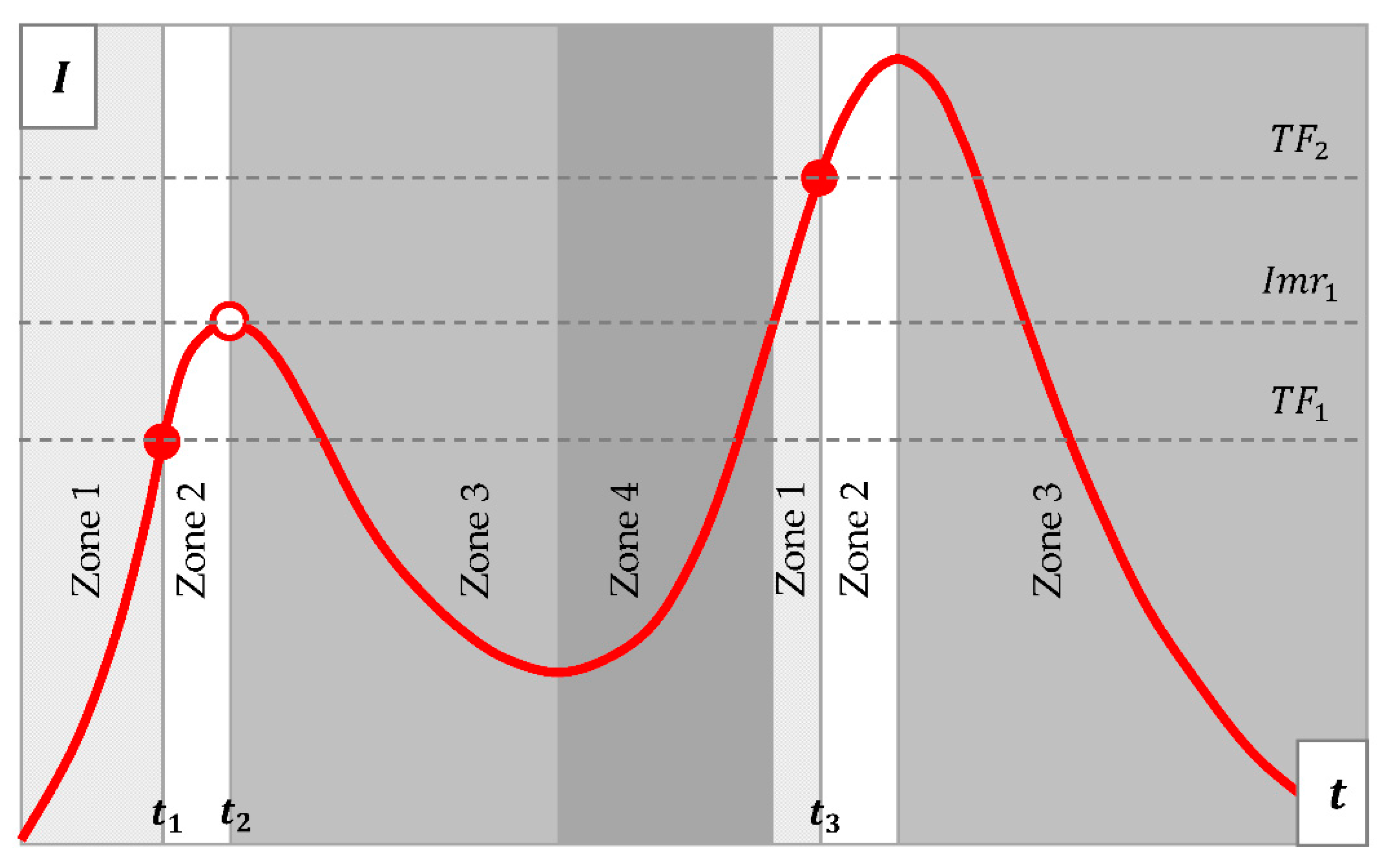
Figure 5 shows an example of the input hydrograph zoning to select the discharge flow. Each zone has a single criterion for selecting the discharge flow. If the input hydrograph has more than one peak value, for each ascending branch, there will be a different threshold flow, T F j .
  • If I t I t 1 0 , that is, if the input flow is maintained or is increasing.
    If I t > max ( I 1 , , I t 1 ) , that is, if a maximum of the input hydrograph has not been reached.
    If I t T F j , that is, if the input flow is less than the threshold value number j [Zone 1].
    O t + i = I t ,
    If I t > T F j , that is, if the input flow is greater than the threshold value number j [Zone 2].
    O t + i = min ( I t , O a v ) ,
    If I t max ( I 1 , , I t 1 ) , that is, if a maximum of the input flow has been reached.
    If I t I m r k , that is, if the inflow to the reservoir is less than or equal to the largest peak of the registered inflow [Zone 4].
    O t + i = min ( I m r k , max ( I t , O a v ) ) ,
    If I t > I m r k , that is, if the inlet flow is greater than the highest recorded inlet flow peak.
    If I t T F j , that is, if the input flow is less than the threshold value number j [Zone 1].
    O t + i = I t ,
    If I t > T F j , that is, if the input flow is greater than the threshold value number j [Zone 2].
    O t + i = min ( I t , O a v ) ,
  • If I t I t 1 < 0 , that is, if the input flow is decreasing [Zone 3].
O t + i = min ( max ( I 1 , , I t 1 ) , O a v ) ,
where:
O t + i : Ouput or discharged flow in the instant t + i , where i is the forecast time interval.
I t : Input flow in the instant t .
T F j : Threshold flow that corresponds to the value of the input flow when a variation less than 1 is reached in the slope of the input hydrograph, where j is the sub-index of the threshold flow recorded up to the current moment.
I m r k : Higher flow peak of the input hydrograph, registered up to the current analysis time t , where k is the sub-index of the peak value recorded up to the current moment.
O a v : Average flow of the forecast probability distribution given by the BNet of flow discharged.

2.8. VEM

In order to compare the results of the BNet model, the VEM [13], a method usually used in Spain, was used. VEM is a reactive-type scheduled management method that works in real-time. At each time step, it calculates the discharge flow based on available surcharge pool volume. This method is based on three fundamental principles: (1) While the inflow is increasing, the discharge flow must be less than the inflow to the reservoir, (2) If the inflow to the reservoir increases, the discharge flow must increase as a function of the previous one, (3) The higher the reservoir level, the greater the percentage increase in the discharge flow relative to the inflow.
At each time step, the method calculates the number of time intervals ( n ) remaining for the available surcharge pool volume ( S t a ) to run out. The volume variation in the reservoir in a time interval Δ t ( Δ S t ) is equal to the difference between the inflow at t ( I t ) and the discharge flow at t 1 ( O t 1 ). If it is considered that the rate of increase in discharged flow is linear, n is:
n = S t a Δ S t = S t a ( I t O t 1 ) · Δ t ,
If a linear increase in the discharge flow is maintained until the surcharge pool volume is exhausted at time Δ t · n , at which point the discharge flow equals the inflow, the discharge flow must increase the following amount in each time interval Δ t :
Δ O t = ( I t O t 1 ) 2 · Δ t S t a ,
The application of the MEV considers 2 parameters: the maximum gradient of discharge flow (MGD) and the activation level (ACT). The MGD is intended to limit damage downstream from the reservoir. In this case, it was assumed equal to the AO. The ACT is an arbitrary value (assumed as 509.3 m [74]), which defines a time interval for the application of the VEM, depending on the zone where the reservoir level is located. If the level is below the TCP, the VEM is applied every 4 h, if it is between the TCP and the ACT level, every 2 h and, if it is above the ACT level, every 1 h.

2.9. Overall Risk Index ( I r )

In order to evaluate the results of the various peak attenuation methods used (VEM, MILP, and BNet), the I r index [21] was calculated. I r is the sum of the risk of damage indexes due to the discharge flow, I 0 , and the risk of damage index due to the storage volume, I S . I 0 is the expected value of damage downstream of the dam, in the areas adjacent to the main water course. I S is the expected value of damage due to overflow on the dam. For each peak attenuation method, the maximum values of discharge flow, O m a x , and storage volume, S m a x , were extracted for each of the N episodes analyzed. Subsequently, the empirical probability of non-exceedance of O m a x and S m a x , F ( O m a x ) and F ( S m a x ) , respectively, was obtained using the Gringorten expression.
I 0 was calculated using the following expression:
I 0 = i = 1 N 1 [ F ( O m a x , i + 1 ) F ( O m a x , i ) ] · D O ( O m a x , i + 1 + O m a x , i 2 ) ,
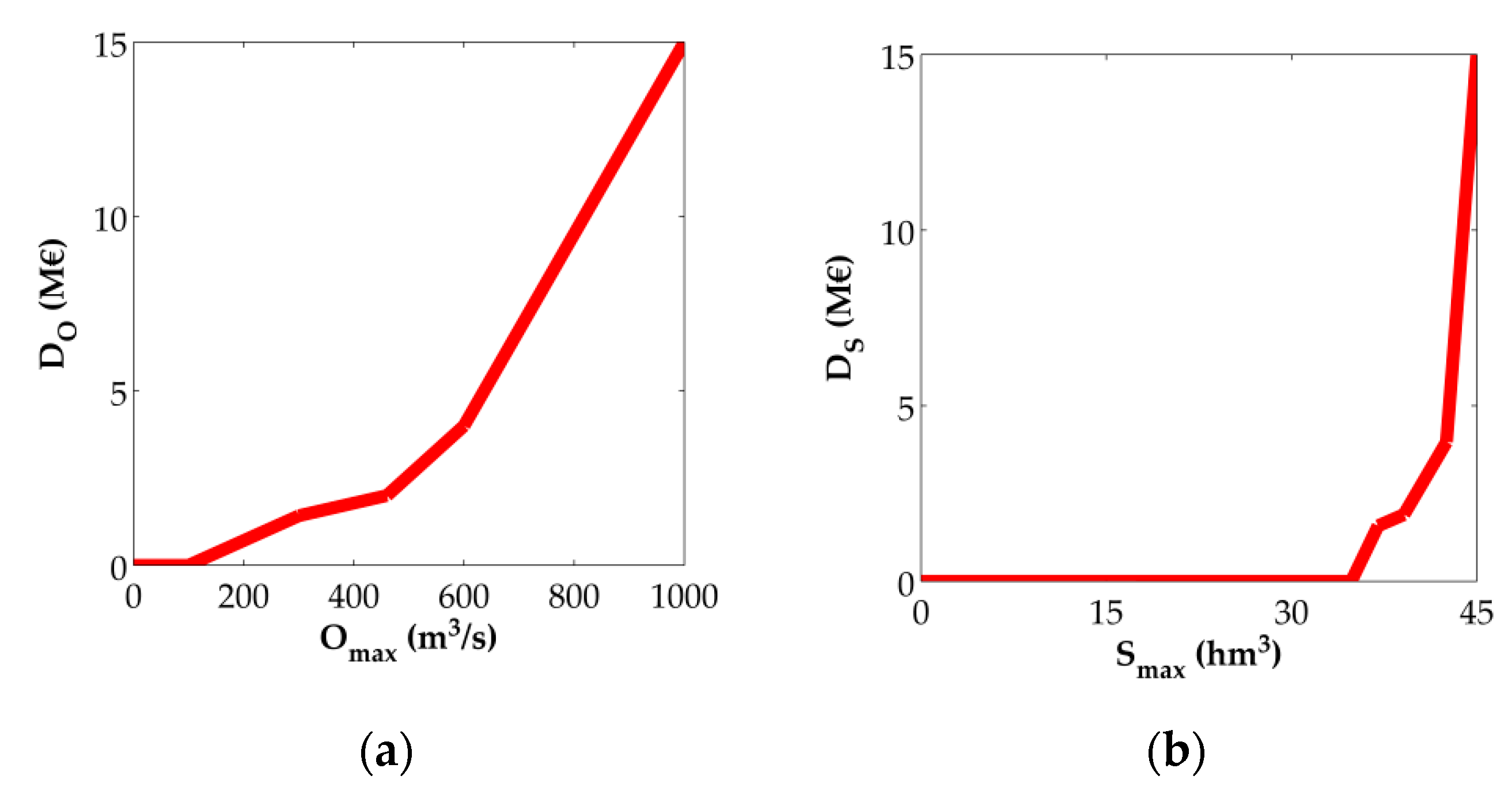
where N is the number of episodes, O m a x , i is the maximum discharged flow in episode i , F ( O m a x , i ) , is the empirical probability of non-exceedance of O m a x , i , and D O , is the damage associated with the maximum discharged flow obtained from the damage curve (Figure 6).
Similarly, I S was calculated using the following expression:
I S = i = 1 N 1 [ F ( S m a x , i + 1 ) F ( S m a x , i ) ] · D S ( S m a x , i + 1 + S m a x , i 2 ) ,
where N is the number of episodes, S m a x , i , is the maximum volume reached by the reservoir in episode i , F ( S m a x , i ) , is the empirical probability of non-exceedance of S m a x , i , and D S , is the damage associated with the maximum volume reached by the reservoir of the damage curve (Figure 7).
The damage curves of the Talave reservoir as proposed by Bianucci et al. [21] were obtained (Figure 7).

3. Results and Discussion

Performance of the BNet
In order to evaluate model performance, the BNet model is compared to two standard models for dam flood operation: the Volumetric Evaluation Model (VEM) and the Mixed Integer Linear Programming (MILP) model. The application of VEM model is the standard practice in many dams in Spain. VEM is a reactive model, which is solely based on the evolution of reservoir level and operates without knowledge of the inflow hydrograph. The results of the VEM model set the baseline for comparison: any proposed model should at least improve the performance of the standard practice. MILP, on the other hand, is taken as the upper limit of model performance. MILP produces a mathematical optimization of dam management, but requires full knowledge of the inflow hydrograph, which is a very unrealistic situation. The results of MILP were used to train the BNet model and thus it can be expected that the performance of the BNet model be lower than that of MILP. The two extreme cases provide a reference to evaluate how BNet can improve over VEM and how far below it is from MILP.
For this purpose, 2000 synthetic hydrographs that enter in the reservoir were generated, as indicated in Section 2.4. The hydrographs were used as inputs to the BNeti ( i = 1, …, 5 h), VEM and MILP models, obtaining, in each case, 2000 time series of reservoir discharge hydrographs and evolution of levels in the reservoir.
When VEM is applied in real-time, the discharge flow and reservoir level are obtained, at each time step of 1 h, during the flood, until reaching TCP level. By applying MILP, a hydrograph of discharge flows and the time series of levels in the reservoir were obtained for each previously known flood. In the case of the BNet, 5 sets of predicted reservoir discharge hydrographs and evolution of levels in the reservoir were obtained, one set for each forecast time interval from 1 to 5 h (Figure 3).
The general procedure to use the BNet requires a brief explanation: First, the BNeti ( i = 1, …, 5 h) was chosen, which, at each instant of time, forecast a discharge flow O t + i (the procedure proposed in Section 2.7 was used, in order to obtain a single predicted discharge flow value at time t + i ). Then, this value was kept until instant t + i 1 was reached, where it becomes the parent node O t . In each time interval the variables I t 1 and I t (parent nodes) are known. With these values the variable Δ I t = I t I t 1 (parent node) was calculated. At each time step the variable W L t (parent node) was calculated using the modified Puls method [75], and, with this value, and W L t 1 , the variable Δ WL t = W L t W L t 1 (parent node) was obtained. Figure 8 shows an example of a real-time BNeti application for i = 3 h.
Applying the BNeti (i = 3 h) in real time, 2000 synthetic episodes were obtained.
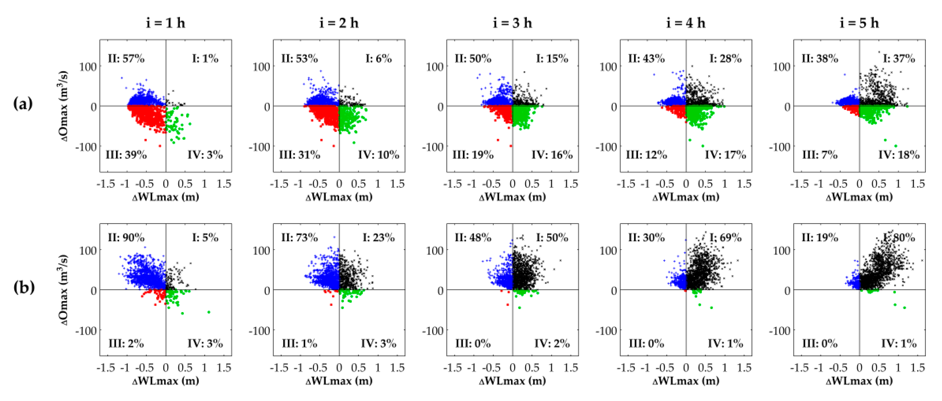
In order to compare the results of the methods, the maximum values of each one of the time series were extracted, corresponding to the maximum discharge flow and the maximum level reached by the reservoir. Subsequently, the differences of the maximum discharge ( Δ O m a x ) and the maximum level reached by the reservoir ( Δ W L m a x ) between the BNeti ( i = 1, …, 5 h) and both, the MILP and VEM comparison methods were calculated. With these results the graphs of Figure 9 and Table 5 were created. On the horizontal axis Δ W L m a x was plotted and on the vertical axis Δ O m a x was plotted.
The objective of this analysis was to know how many episodes resulted in lower O m a x and W L m a x when using the BNeti ( i = 1, …, 5 h) than when using VEM and MILP methods.
Δ W L m a x and Δ O m a x values can be positive or negative.
If Δ O m a x > 0 , the O m a x values of the BNeti are greater than those of the comparison method (MILP or VEM), therefore, the BNeti generates a smaller peak attenuation. If Δ O m a x < 0 , the opposite happens.
If Δ W L m a x > 0 , the W L m a x values of the BNeti are greater than those of the comparison method (MILP or VEM). If Δ W L m a x < 0 , the opposite happens.
The Δ O m a x and Δ W L m a x values can be combined as follows:
If Δ O m a x > 0 and Δ W L m a x > 0 , the O m a x and W L m a x values of an episode that result with the BNeti are greater than the values obtained from the standard method (VEM or MILP). In this case, the episode analyzed falls into quadrant I of Figure 9.
If Δ O m a x > 0 and Δ W L m a x < 0 , the analyzed episode belongs to quadrant II of Figure 9.
If Δ O m a x < 0 and Δ W L m a x < 0 , the analyzed episode belongs to quadrant III of Figure 9.
If Δ O m a x < 0 and Δ W L m a x > 0 , the analyzed episode belongs to quadrant IV of Figure 9.
Figure 9a ( i = 1 h) shows that in 39% of the events, the results of maximum discharge and maximum level reached by the reservoir, when using the BNeti ( i = 1 h), are simultaneously lower than those obtained using the VEM, meanwhile, only 1% are larger. In 57% of the episodes, the maximum flows discharged using the BNeti ( i = 1 h) are greater than those obtained using the VEM, while the maximum levels are lower. In 3% of the episodes, the maximum levels reached using the BNeti ( i = 1 h) are greater than those obtained using the VEM, while the maximum discharges are lower.
Table 5 and Figure 9a show that when comparing the BNet (for 5 forecast time steps) with the VEM, as the BNet forecast time increases, the number of episodes decrease in quadrant III, increase in quadrant I, decrease in quadrant II, and increase in quadrant IV. The decrease in the number of episodes in quadrant III means that O m a x and W L m a x calculated with the BNet are increasingly greater than those calculated with VEM. The increase in the number of episodes in quadrant I means that the O m a x and W L m a x calculated with the BNet are increasingly greater than those calculated with the VEM. The decrease in the number of episodes in quadrant II means that the O m a x calculated with the BNet are increasingly lower than those calculated with the VEM. The increase in the number of episodes in quadrant IV means that the maximum levels calculated with the BNet are increasingly higher than those calculated with the VEM.
Figure 9a shows that in the first three forecast time intervals, i = 1, 2, and 3 h, BNet results are better than VEM, since there are more episodes in quadrant III than in quadrant I. On the contrary, in the forecast time intervals, i = 4 and 5 h, VEM results are better than BNet, since there are more episodes in quadrant I than in quadrant III.
Figure 9b (i = 1 h) shows that 2% of the events of the BNet simultaneously returns lower values of maximum discharge and maximum level than the MILP. On the contrary, in 6% of the cases, the MILP returns higher results of the comparison variables than the BNet. In 90% of the cases, the BNet returns higher values of maximum flow discharged and lower maximum levels, than the MILP. Finally, in 3% of the episodes, the BNet returns lower values of maximum flow discharged and higher levels than the MILP.
Figure 9b shows that in all forecast time intervals, MILP returns better results than VEM.
This result is explained by the fact that the set of values of both the MILP and the VEM methods, which are used to compare with the BNet, is always the same, regardless of the forecast time step. For each episode, both MILP and VEM return a single hydrograph and a single time series of evolution of levels in the reservoir, from which the maximum values of discharge flow and level reached are extracted, which are then used to compare with the BNet. In the case of MILP, this is possible because the hydrographs entering the reservoir are known before applying this method. On the other hand, the BNet decreases the forecast quality as the forecast time step increases (see Table 4). Given that MILP provides the optimal results with which the BNet is trained, it is expected that its results will be better than the BNet. The BNet, relative to VEM, is always at a “disadvantage”, since the predicted future results of the BNet are compared with the results of the VEM, which is unable to forecast. Even so, better results are obtained with the BNet than with the VEM up to i = 3 h, and worse, from i = 4 h.
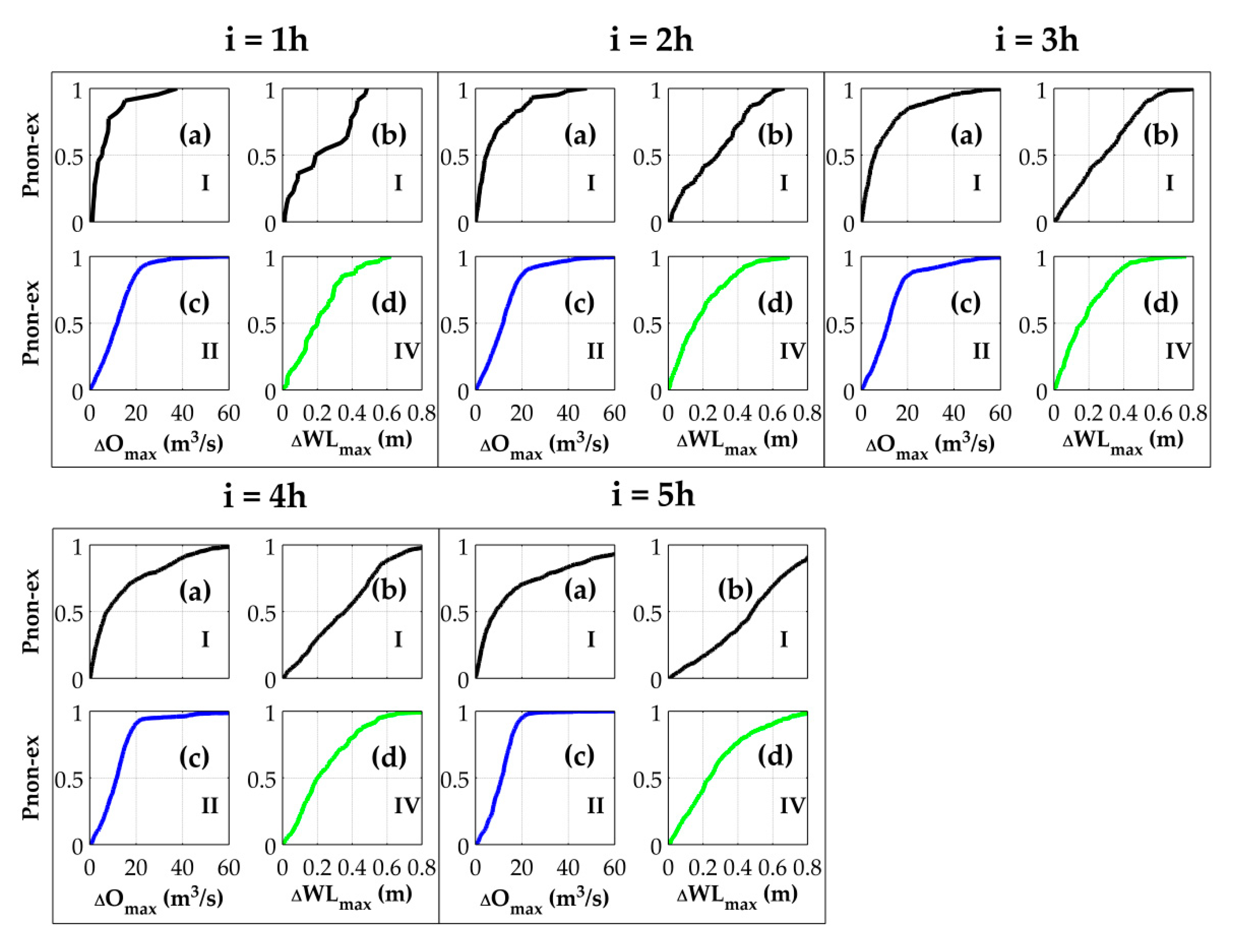
For the episodes outside of quadrant III, it was analyzed how far the results obtained with the BNeti ( i = 1, …, 5 h) are from those generated with the VEM. For this, a graph of the probability of non-exceedance of the maximum differences Δ O m a x and Δ W L m a x , was created, in each BNeti ( i = 1, …, 5 h) of the episodes that belong to quadrants I, II, and IV (Figure 10).
Figure 10 shows the percentages of episodes found in quadrants I, II, and IV for different thresholds. The greater the number of episodes under small thresholds, the greater the similarities between the results of both methods (VEM and BNet). In quadrant II, it should be highlighted the difference in maximum discharge ( Δ O m a x ), and in quadrant IV the maximum level difference ( Δ W L m a x ). In quadrant I it is important to highlight the thresholds corresponding to the difference in maximum discharge ( Δ O m a x ) and to the difference in the maximum level reached by the reservoir ( Δ W L m a x ).
Figure 10 ( i = 1 h) shows that in quadrant II(c), with a probability of non-exceedance of 0.9, the differences in Δ O m a x do not exceed 21.3 m3/s, which is only the 13% percentile of the O m a x resulting from the VEM and the BNeti ( i = 1 h). In quadrant IV(d), with a probability of non-exceedance of 0.9, the Δ W L m a x do not exceed 0.42 m, which is the 36% percentile of the W L m a x reached by the reservoir resulting from the VEM and the BNeti ( i = 1 h). In quadrant I, which concentrates the results in which the VEM behaves better than the BNeti ( i = 1 h), with a probability of non-exceedance of 0.9, Δ O m a x (a) do not exceed 15 m3/s, which is only the 9% percentile, and Δ W L m a x (b) do not exceed 0.43 m, which is at the 37% percentile.
In quadrant I(a), as the BNet forecast time advances, for the same probability of non-exceedance, Δ O m a x increases, that is, the value of O m a x calculated with the BNet increases its difference with respect to the value calculated with the VEM. In quadrant I(b), as the BNet forecast time advances, for the same probability of non-exceedance, Δ W L m a x increases, that is, the value of W L m a x calculated with the BNet increases its difference with respect to the value calculated with the VEM. In quadrant II(c), there is no significant difference between the non-exceedance probability curves as the BNet forecast time progresses. In quadrant IV(d), there is also no significant difference between the non-exceedance probability curves as the BNet forecast time progresses.
An analysis of the variables O m a x and W L m a x was also performed separately, plotting their probabilities of non-exceedance in each of the forecast time intervals (from i = 1 to 5 h) by applying the BNet, VEM, and MILP methods. Figure 11a shows that the probability of non-exceedance of the O m a x calculated with the BNeti ( i = 1, …, 5 h) is lower than that calculated with the VEM and the MILP, up to the AO. Above EO, the probability of non-exceedance of the O m a x calculated with the BNet is lower than the probabilities of non-exceedance of the VEM and the MILP. Between AO and EO, the values of probability of non-exceedance of the O m a x calculated with the BNet are intermediate between VEM and MILP values, with a tendency to match the VEM as the BNet forecast interval increases.
Figure 11b shows that as the BNet forecast time increases, the probability of non-exceedance of the W L m a x tends to decrease. For the BNeti ( i = 1 h), the probability of non-exceedance of the W L m a x is greater than that calculated with the MILP and VEM methods.
In order to compare the BNet results with the VEM, from the point of view of risk reduction, the global risk index ( I r ) [21] was calculated, which simultaneously quantifies the overflow risk of the dam ( I S ) and the flood risk downstream of the dam ( I O ), such as, I r   =   I S   +   I O (Table 6).
Table 6 shows that the downstream flood risk ( I O ) calculated with the BNeti ( i = 1, …, 3 h) that forecast the discharged flow from 1 h to 3 h, was lower than the risk of VEM. Likewise, the overflow risk ( I S ) obtained with the BNeti ( i = 1 h) that forecast the discharged flow in 1 h, was lower than the risk of VEM. Finally, the overall risk ( I r ) calculated with the BNeti ( i = 1 and 2 h) that forecast the discharged flow in an interval of 1 h and 2 h, was lower than the VEM overall risk.
VEM is a reactive method for managing reservoirs in floods that makes a single discharge decision at each instant of time depending on the state of the reservoir. This method works in real-time, but does not forecast. For the 2000 synthetic reservoir input hydrographs, VEM returned a single set of 2000 combinations of maximum discharge flows and maximum levels reached by the reservoir, with which I r was calculated.
MILP is a method that optimizes the management of the reservoir in floods that requires knowing the entire hydrograph that enters the reservoir before being applied, therefore, its use in real-time is very limited. For the 2000 synthetic reservoir input hydrographs, MILP returned a single set of 2000 combinations of maximum discharge flows and maximum levels reached by the reservoir, with which I r was calculated.
The BNet was applied for the 2000 synthetic hydrographs entering the reservoir, for 5 forecast time steps (see Figure 8), obtaining, for each forecast time step, a different set of 2000 combinations of maximum discharge flows and maximum levels reached by the reservoir. I r was calculated for each of the 5 data sets.
The BNet was trained with the results of the MILP, so it is expected that the results of the BNet are worse than those of the MILP, which is consistent with the value of the I r calculated (Table 6).
On the other hand, the forecast quality of the BNet decreases as the forecast time step increases (Table 4), so I r increases with the forecast time step. For the first 2 forecast time steps, the I r of the BNet is less than the I r of the VEM (which is unique), but, from the 3-h forecast time step, I r of theBNeti (i = 3, …, 5 h) exceeds that of the VEM. These results are explained because the BNet predicts and VEM does not, so the BNet always compares at a “disadvantage”.
In a practical case of real-time application, the BNet could be used to forecast the flow discharged by the dam in all time horizons, from 1 to 5 h, obtaining 5 probable values of future discharge flows, one for each forecast time step, values that the VEM is unable to estimate.

4. Conclusions

The proposed methodology is useful to build a decision-support system for dam operation during floods based on the Bayesian model. The analyses performed showed that the Bayesian model can improve the performance of the VEM model, which is the method of choice for real time operation in many dams in Spain. More sophisticated optimization models, like MILP, cannot be easily applied in real time because they require full knowledge of the inflow hydrograph. These models, however, can be used to produce a large dataset of optimal dam operations that can be used to train the BNet. The Bayesian model can thus be used in real time without the need for a hydrograph forecast module.
The developed BNet model predicts the flow discharged through the reservoir outlets during floods over a time horizon of 1 to 5 h. This model adapted the MILP model that optimizes the management of the reservoir, but it cannot be easily used in real-time. In order to evaluate the learning process of the BNet its quality attributes were calculated: area under the ROC curve and RPS index. The area under the ROC curve varied between 0.973, for 1 h of forecast, and 0.956, for 5 h, values close to 1 that show the ability of the BNet. The RPS index varied between 0.006 and 0.017, for 1 h of forecast and 5 h, respectively, values close to 0, which indicate that the BNet returns good results with respect to this attribute. The values of both attributes show that the BNet learning process was satisfactory.
Since the BNet returns the most probable class interval of the predicted discharge flow, a selection method of a single forecast value at each instant of time was proposed, in order to facilitate the use of the BNet by the dam operator.
The BNet model was compared with the MILP method, which cannot be easily applied in real-time, and with the VEM, which works in real-time, but does not forecast. The values of maximum discharge flow and maximum level reached by the reservoir, calculated by each method, were extracted. Based on these values, the overall risk index ( I r ) was estimated, obtaining 0.383 M€ for MILP, which is the lower limit, and 0.551 M€ for VEM. The BNet returned an I r value of 0.445 M€ for 1 h forecast, 0.533 M€ for 2 h, 0.653 M€ for 3 h, 0.834 M€ for 4 h, and 1.006 M€ for 5 h. Therefore, it was concluded that the BNet presented better results than the VEM, which does not predict, even for BNet forecast time steps of up to 2 h. Finally, this model improves the results from one of the most used methods in Spain, the VEM, and could represent and improvement to the actual dam operation methods.

Author Contributions

Conceptualization, V.C.-V., L.G., J.H.G.-P., A.S.-W. and P.B.; methodology, V.C.-V., L.G., J.H.G.-P., A.S.-W. and P.B.; software, V.C.-V.; formal analysis, V.C.-V., L.G., A.S.-W., J.H.G.-P. and P.B.; investigation, V.C.-V., J.H.G.-P., A.S.-W. and L.G.; resources, J.H.G.-P. and L.G.; data curation, V.C.-V.; writing—original draft preparation, V.C.-V.; writing—review and editing, V.C.-V., A.S.-W., L.G., P.B. and J.H.G.-P.; visualization, V.C.-V.; funding acquisition, L.G. All authors have read and agreed to the published version of the manuscript.

Funding

This manuscript was supported by funding from: the Spanish Ministry of Science and Innovation (SECA-SRH; Ref. PID2019-105852RA-I00); and the Fundación Agustín de Betancourt through a PhD student grant. The first author acknowledges the financial support provided by Universidad Politecnica de Madrid through its Latin America doctoral student mobility program.

Acknowledgments

The authors wish to thank Confederación Hidrografica del Segura for providing hydrological data for the Talave dam through its Automatic Hydrological Information System.

Conflicts of Interest

The authors declare no conflict of interest.

References

  1. Barman, S.D.; Choudhury, P. Downstream Flood Peak Improvement Modeling for a River System Incorporating Ungauged Subbasins. Aquat. Procedia 2015, 4, 1189–1196. [Google Scholar] [CrossRef]
  2. Zhan, X.; Qin, H.; Liu, Y.; Yao, L.; Xie, W.; Liu, G.; Zhou, J. Variational Bayesian Neural Network for Ensemble Flood Forecasting. Water 2020, 12, 2740. [Google Scholar] [CrossRef]
  3. Feng, M.; Liu, P. Spillways Scheduling for Flood Control of Three Gorges Reservoir Using Mixed Integer Linear Programming Model. Math. Probl. Eng. 2014, 2014, e921767. [Google Scholar] [CrossRef]
  4. Pan, L.; Housh, M.; Liu, P.; Cai, X.; Chen, X. Robust stochastic optimization for reservoir operation. Water Resour. Res. 2015, 51, 409–429. [Google Scholar] [CrossRef] [Green Version]
  5. Wang, L.; Nyunt, C.T.; Koike, T.; Saavedra, O.; Nguyen, L.C.; van Sap, T. Development of an integrated modeling system for improved multi-objective reservoir operation. Front. Archit. Civ. Eng. China 2010, 4, 47–55. [Google Scholar] [CrossRef]
  6. Wurbs, R.A. Comparative Evaluation of Generalized River/Reservoir System Models; Texas Water Resources Institute: College Station, TX, USA, 2005. [Google Scholar]
  7. Ahmadi, M.; Bozorg Haddad, O.; Mariño, M.A. Extraction of Flexible Multi-Objective Real-Time Reservoir Operation Rules. Water Resour. Manag. 2014, 28, 131–147. [Google Scholar] [CrossRef]
  8. Li, Y.; Guo, S.; Guo, J.; Wang, Y.; Li, T.; Chen, J. Deriving the optimal refill rule for multi-purpose reservoir considering flood control risk. J. Hydro Environ. Res. 2014, 8, 248–259. [Google Scholar] [CrossRef]
  9. Farhangi, M.; Bozorg-Haddad, O.; Mariño, M.A. Evaluation of simulation and optimization models for WRP with PIs. In Proceedings of the Institution of Civil Engineers-Water Management; Thomas Telford Ltd.: London, UK, 2012; Volume 165, pp. 265–276. [Google Scholar] [CrossRef]
  10. Molina, M.; Fuentetaja, R.; Garrote, L. Hydrologic Models for Emergency Decision Support Using Bayesian Networks. In Proceedings of the Symbolic and Quantitative Approaches to Reasoning with Uncertainty, Barcelona, Spain, 6–8 July 2005; Godo, L., Ed.; Springer: Berlin/Heidelberg, Germany, 2005; pp. 88–99. [Google Scholar]
  11. Chen, J.; Zhong, P.; Xu, B.; Zhao, Y. Risk Analysis for Real-Time Flood Control Operation of a Reservoir. J. Water Resour. Plan. Manag. 2015, 141, 04014092. [Google Scholar] [CrossRef]
  12. Bianucci, P.; Sordo-Ward, Á.; Moralo, J.; Garrote, L. Probabilistic-Multiobjective Comparison of User-Defined Operating Rules. Case Study: Hydropower Dam in Spain. Water 2015, 7, 956–974. [Google Scholar] [CrossRef] [Green Version]
  13. Girón, F. The evacuation of Floods during the Operation of Reservoirs. In Transactions Sixteenth International Congress on Large Dams; Report 75; International Commission on Large Dams (ICOLD): San Francisco, CA, USA, 1988; Volume 4, pp. 1261–1283. [Google Scholar]
  14. Chen, J.; Zhong, P.; Wang, M.; Zhu, F.; Wan, X.; Zhang, Y. A Risk-Based Model for Real-Time Flood Control Operation of a Cascade Reservoir System under Emergency Conditions. Water 2018, 10, 167. [Google Scholar] [CrossRef] [Green Version]
  15. Gioia, A. Reservoir Routing on Double-Peak Design Flood. Water 2016, 8, 553. [Google Scholar] [CrossRef] [Green Version]
  16. Liu, P.; Lin, K.; Wei, X. A two-stage method of quantitative flood risk analysis for reservoir real-time operation using ensemble-based hydrologic forecasts. Stoch. Environ. Res. Risk Assess. 2015, 29, 803–813. [Google Scholar] [CrossRef]
  17. Choong, S.-M.; El-Shafie, A. State-of-the-Art for Modelling Reservoir Inflows and Management Optimization. Water Resour. Manag. 2015, 29, 1267–1282. [Google Scholar] [CrossRef]
  18. Hossain, M.S.; El-shafie, A. Intelligent Systems in Optimizing Reservoir Operation Policy: A Review. Water Resour. Manag. 2013, 27, 3387–3407. [Google Scholar] [CrossRef]
  19. El-Shafie, A.; El-Shafie, A.H.; Mukhlisin, M. New Approach: Integrated Risk-Stochastic Dynamic Model for Dam and Reservoir Optimization. Water Resour. Manag. 2014, 28, 2093–2107. [Google Scholar] [CrossRef]
  20. Hosseini-Moghari, S.-M.; Morovati, R.; Moghadas, M.; Araghinejad, S. Optimum Operation of Reservoir Using Two Evolutionary Algorithms: Imperialist Competitive Algorithm (ICA) and Cuckoo Optimization Algorithm (COA). Water Resour. Manag. 2015, 29, 3749–3769. [Google Scholar] [CrossRef]
  21. Bianucci, P.; Sordo-Ward, A.; Pérez, J.I.; García-Palacios, J.; Mediero, L.; Garrote, L. Risk-based methodology for parameter calibration of a reservoir flood control model. Nat. Hazards Earth Syst. Sci. 2013, 13, 965–981. [Google Scholar] [CrossRef] [Green Version]
  22. Heydari, M.; Othman, F.; Qaderi, K. Developing Optimal Reservoir Operation for Multiple and Multipurpose Reservoirs Using Mathematical Programming. Math. Probl. Eng. 2015, 2015, e435752. [Google Scholar] [CrossRef]
  23. Rani, D.; Moreira, M.M. Simulation–Optimization Modeling: A Survey and Potential Application in Reservoir Systems Operation. Water Resour. Manag. 2010, 24, 1107–1138. [Google Scholar] [CrossRef] [Green Version]
  24. Labadie John, W. Optimal Operation of Multireservoir Systems: State-of-the-Art Review. J. Water Resour. Plan. Manag. 2004, 130, 93–111. [Google Scholar] [CrossRef]
  25. Yeh, W.W.-G. Reservoir Management and Operations Models: A State-of-the-Art Review. Water Resour. Res. 1985, 21, 1797–1818. [Google Scholar] [CrossRef]
  26. Wurbs Ralph, A. Reservoir-System Simulation and Optimization Models. J. Water Resour. Plan. Manag. 1993, 119, 455–472. [Google Scholar] [CrossRef]
  27. Afshar, A.; Mariño, M.A. Multi-objective Coverage-based ACO Model for Quality Monitoring in Large Water Networks. Water Resour. Manag. 2012, 26, 2159–2176. [Google Scholar] [CrossRef]
  28. Díaz, F.J.; Contreras, J.; Muñoz, J.I.; Pozo, D. Optimal Scheduling of a Price-Taker Cascaded Reservoir System in a Pool-Based Electricity Market. IEEE Trans. Power Syst. 2011, 26, 604–615. [Google Scholar] [CrossRef]
  29. Windsor, J.S. Optimization model for the operation of flood control systems. Water Resour. Res. 1973, 9, 1219–1226. [Google Scholar] [CrossRef]
  30. Needham Jason, T.; Watkins David, W.; Lund Jay, R.; Nanda, S.K. Linear Programming for Flood Control in the Iowa and Des Moines Rivers. J. Water Resour. Plan. Manag. 2000, 126, 118–127. [Google Scholar] [CrossRef] [Green Version]
  31. Beneyto, C.; Aranda, J.A.; Benito, G.; Francés, F. Metodología basada en generadores meteorológicos para la estimación de avenidas extremas. Ingeniería del Agua 2019, 23, 259–273. [Google Scholar] [CrossRef]
  32. Ahmed, E.-S.M.S.; Mays, L.W. Model for determining real-time optimal dam releases during flooding conditions. Nat. Hazards 2013, 65, 1849–1861. [Google Scholar] [CrossRef]
  33. Jones, D. Application of Mixed-Integer Programming for Flood Control in the Sacramento Valley: Insights & Limitations. Master’s Thesis, University of California, Davis, CA, USA, 1999. [Google Scholar]
  34. Wei, C.-C.; Hsu, N.-S. Multireservoir real-time operations for flood control using balanced water level index method. J. Environ. Manag. 2008, 88, 1624–1639. [Google Scholar] [CrossRef]
  35. Che, D.; Mays, L.W. Application of an Optimization/Simulation Model for Real-Time Flood-Control Operation of River-Reservoirs Systems. Water Resour. Manag. 2017, 31, 2285–2297. [Google Scholar] [CrossRef]
  36. Mediero, L.; Garrote, L.; Martín-Carrasco, F. A probabilistic model to support reservoir operation decisions during flash floods. Hydrol. Sci. J. 2007, 52, 523–537. [Google Scholar] [CrossRef] [Green Version]
  37. Gabriel-Martin, I.; Sordo-Ward, A.; Garrote, L.; Castillo, L.G. Influence of initial reservoir level and gate failure in dam safety analysis. Stochastic approach. J. Hydrol. 2017, 550, 669–684. [Google Scholar] [CrossRef]
  38. Khalil, A.; McKee, M.; Kemblowski, M.; Asefa, T. Sparse Bayesian learning machine for real-time management of reservoir releases. Water Resour. Res. 2005, 41. [Google Scholar] [CrossRef]
  39. Zacchei, E.; Molina, J.L. Shape Optimization of Double-Arch Dams by Using Parameters Obtained Through Bayesian Estimators. Iran. J. Sci. Technol. Trans. Civ. Eng. 2019, 43, 649–662. [Google Scholar] [CrossRef]
  40. Zacchei, E.; Molina, J.L. Optimization of Geometric Parameters for Double-Arch Dams through Bayesian Implementation. J. Struct. Eng. 2020, 146, 04020264. [Google Scholar] [CrossRef]
  41. Vogel, K.; Weise, L.; Schröter, K.; Thieken, A.H. Identifying Driving Factors in Flood-Damaging Processes Using Graphical Models. Water Resour. Res. 2018, 54, 8864–8889. [Google Scholar] [CrossRef]
  42. Molina, J.-L.; Zazo, S.; Martín, A.-M. Causal Reasoning: Towards Dynamic Predictive Models for Runoff Temporal Behavior of High Dependence Rivers. Water 2019, 11, 877. [Google Scholar] [CrossRef] [Green Version]
  43. Molina, J.-L.; Zazo, S. Assessment of Temporally Conditioned Runoff Fractions in Unregulated Rivers. J. Hydrol. Eng. 2018, 23, 04018015. [Google Scholar] [CrossRef]
  44. Wu, J.; Fang, W.; Hu, Z.; Hong, B. Application of Bayesian Approach to Dynamic Assessment of Floodin Urban Underground Spaces. Water 2018, 10, 1112. [Google Scholar] [CrossRef] [Green Version]
  45. Wang, J.; Liang, Z.; Jiang, X.; Li, B.; Chen, L. Bayesian Theory Based Self-Adapting Real-Time Correction Model for Flood Forecasting. Water 2016, 8, 75. [Google Scholar] [CrossRef] [Green Version]
  46. Cu Thi, P.; Ball, J.; Dao, N. Uncertainty Estimation Using the Glue and Bayesian Approaches in Flood Estimation: A case Study—Ba River, Vietnam. Water 2018, 10, 1641. [Google Scholar] [CrossRef] [Green Version]
  47. Malekmohammadi, B.; Kerachian, R.; Zahraie, B. Developing monthly operating rules for a cascade system of reservoirs: Application of Bayesian Networks. Environ. Model. Softw. 2009, 24, 1420–1432. [Google Scholar] [CrossRef]
  48. Li, P.; Liang, C. Risk Analysis for Cascade Reservoirs Collapse Based on Bayesian Network sunder the Combined Action of Flood and Land slide Surge. Math. Probl. Eng. 2016, 2016, 1–13. [Google Scholar] [CrossRef]
  49. Chen, J.; Zhong, P.-A.; An, R.; Zhu, F.; Xu, B. Risk analysis for real-time flood control operation of a multi-reservoir system using a dynamic Bayesian network. Environ. Model. Softw. 2019, 111, 409–420. [Google Scholar] [CrossRef]
  50. Lu, Q.; Zhong, P.; Xu, B.; Zhu, F.; Ma, Y.; Wang, H.; Xu, S. Risk analysis for reservoir flood control operation considering two-dimensional uncertainties based on Bayesian network. J. Hydrol. 2020, 589, 125353. [Google Scholar] [CrossRef]
  51. Chen, Y.; Lin, P. Bayesian network of risk assessment for a super-large dam exposed to multiple natural risk sources. Stoch. Environ. Res. Risk Assess. 2019, 33, 581–592. [Google Scholar] [CrossRef]
  52. Neapolitan, R.E. Learning Bayesian Networks; Prentice-Hall, Inc.: Upper Saddle River, NJ, USA, 2003; ISBN 978-0-13-012534-7. [Google Scholar]
  53. Stephenson, T.A. An Introduction to Bayesian Network Theory and Usage; IDIAP: Valais, Switzerland, 2000. [Google Scholar]
  54. Lauritzen, S.L. The EM algorithm for graphical association models with missing data. Comput. Stat. Data Anal. 1995, 19, 191–201. [Google Scholar] [CrossRef]
  55. Sordo-Ward, A.; Garrote, L.; Martín-Carrasco, F.; Dolores Bejarano, M. Extreme flood abatement in large dams with fixed-crest spillways. J. Hydrol. 2012, 466–467, 60–72. [Google Scholar] [CrossRef] [Green Version]
  56. Sordo-Ward, A.; Garrote, L.; Bejarano, M.D.; Castillo, L.G. Extreme flood abatement in large dams with gate-controlled spillways. J. Hydrol. 2013, 498, 113–123. [Google Scholar] [CrossRef]
  57. Etoh, T.; Murota, A.; Nakanishi, M. SQRT-Exponential Type Distribution of Maximum. In Proceedings of the Hydrologic Frequency Modeling, Louisiana State University, Baton Rouge, MS, USA, 14–17 May 1986; Singh, V.P., Ed.; Springer: Dordrecht, The Netherlands, 1987; pp. 253–264. [Google Scholar]
  58. Ministerio de Fomento. Máximas Lluvias Diarias en la España Peninsular; Dirección General de Carreteras: Madrid, España, 1999.
  59. Ministerio de Obras Públicas y Urbanismo (MOPU). Instrucción de Carreteras 5.2-IC Drenaje Superficial; Dirección General de Carreteras: Madrid, España, 1990.
  60. Spanish National Committee on Large Dams (SPANCOLD). Guía Técnica de Seguridad de Presas N°4; Avenida de Proyecto: Madrid, Spain, 1997. [Google Scholar]
  61. Bras, R.L.; Rodriguez-Iturbe, I. Random Functions and Hydrology; Dover Publications: New York, NY, USA, 1994; ISBN 978-0-486-67626-5. [Google Scholar]
  62. Toth, E.; Brath, A.; Montanari, A. Comparison of short-term rainfall prediction models for real-time flood forecasting. J. Hydrol. 2000, 239, 132–147. [Google Scholar] [CrossRef]
  63. Bocchiola, D.; Rosso, R. The use of scale recursive estimation for short term quantitative precipitation forecast. Phys. Chem. Earth Parts A/B/C 2006, 31, 1228–1239. [Google Scholar] [CrossRef]
  64. De Salas, L.; Fernández, J.A. “In-site” regionalization to estimate an intensity-duration-frequency law: A solution to scarce spatial data in Spain. Hydrol. Process. 2007, 21, 3507–3513. [Google Scholar] [CrossRef]
  65. Rodríguez-Iturbe, I.; de Power, B.F.; Valdés, J.B. Rectangular pulses point process models for rainfall: Analysis of empirical data. J. Geophys. Res. 1987, 92, 9645. [Google Scholar] [CrossRef]
  66. Mockus, V. Chapter 21. Design Hydrographs. In National Engineering Handbook, Section 4, Hydrology; SCS, Ed.; SCS: Washington, DC, USA, 1972. [Google Scholar]
  67. McCarthy, G.T. The unit hydrograph and flood routing. In Proceedings of the Conference of North Atlantic Division; US Army Corps of Engineers: Vicksburg, MS, USA, 1938; pp. 608–609. [Google Scholar]
  68. Herskovits, E.H.; Cooper, G.F. Kutato: An Entropy-Driven System for Construction of Probabilistic Expert Systems from Databases; Knowledge Systems Laboratory, Medical Computer Science; Stanford University: Stanford, CA, USA, 1990. [Google Scholar]
  69. Romero Díaz, A.; Maurandi Guirado, A. Las inundaciones en la cuenca del Segura en las dos últimas décadas del siglo XX: Actuaciones de prevención. Ser. Geogr. 2000, 9, 93–120. [Google Scholar]
  70. Carvajal, C.; Peyras, L.; Arnaud, P.; Boissier, D.; Royet, P. Probabilistic Modeling of Flood water Level for Dam Reservoirs. J. Hydrol. Eng. 2009, 14, 223–232. [Google Scholar] [CrossRef]
  71. Gabriel-Martin, I.; Sordo-Ward, A.; Garrote, L. Influencia del nivel inicial en la definición de resguardos estacionales en presas. Ingeniería del Agua 2018, 22, 225–238. [Google Scholar] [CrossRef]
  72. Mason, S.J.; Graham, N.E. Conditional Probabilities, Relative Operating Characteristics, and Relative Operating Levels. Weather Forecast. 1999, 14, 14. [Google Scholar] [CrossRef]
  73. Wilks, D.S. Statistical Methods in the Atmospheric Sciences; Academic Press: Cambridge, MA, USA, 2011; ISBN 978-0-12-385022-5. [Google Scholar]
  74. Sordo-Ward, A.; Gabriel-Martin, I.; Bianucci, P.; Garrote, L. A Parametric Flood Control Method for Dams with Gate-Controlled Spillways. Water 2017, 9, 237. [Google Scholar] [CrossRef] [Green Version]
  75. Chow, V.T. Handbook of Applied Hydrology: A Compendium of Water-Resources Technology, 1st ed.; McGraw-Hill: New York, NY, USA, 1964; ISBN 978-0-07-010774-8. [Google Scholar]
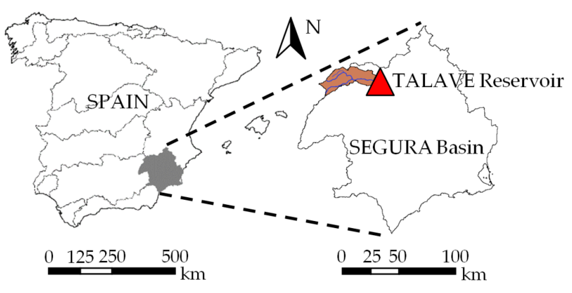
Figure 1. Location of Talave dam in the Segura River Basin.
Water 12 03206 g001
Figure 2. Evolution of the conditional entropy for the 50,000 episodes used in the training and evaluation of the BNet.
Water 12 03206 g002
Figure 3. BNet structure that forecast the discharge flow of the reservoir at time t   +   i hours, where i =   1 to 5 h.
Water 12 03206 g003
Figure 4. Slope ratio ( k t ) of the input hydrograph to the reservoir between two consecutive time intervals.
Water 12 03206 g004
Figure 5. Zoning based on the input hydrograph to the reservoir of a single criterion for selecting the flow discharged in each zone, according to Figure 6 and the following steps:
Water 12 03206 g005
Figure 6. Scheme of the selection procedure of the forecast discharge flow according to the zoning of the input hydrograph.
Water 12 03206 g006
Figure 7. Damage curves due to (a) discharge flow and (b) storage volume of the Talave reservoir [21].
Water 12 03206 g007
Figure 8. Real-time application of the BNeti ( i = 3 h).
Water 12 03206 g008
Figure 9. Comparison of the BNet results for each forecast time step ( i = 1 to 5 h) with the Volumetric Evaluation Method (VEM) (a) and mixed integer linear programming (MILP) (b) for 2000 synthetic episodes of flood.
Water 12 03206 g009
Figure 10. Probability of non-exceedance of the differences in maximum discharged flows ( Δ O m a x ) and the maximum levels reached by the reservoir ( Δ W L m a x ), between the VEM and the BNeti ( i = 1, …, 5 h), in quadrants I, II, and IV.
Water 12 03206 g010
Figure 11. Probabilities of non-exceedance of: (a) maximum discharge flows ( O m a x ) and (b) maximum levels ( W L m a x ), obtained with the VEM, MILP, and BNeti (i = 1, …, 5 h).
Water 12 03206 g011
Table 1. Talave Dam characteristics. Levels and storage capacity.
SymbolDescriptionWater Level (m)Volume (hm3)
TCPTop of conservation pool
(maximum normal operative level)
508.931.9
FCLFlood control level (top of flood control pool)509.934.8
DFLDesign flood level511.339.1
TOPTop of dam512.442.5
Table 2. Downstream river characteristic capacity (flows).
SymbolDescriptionFlow (m3/s)
AOAlert outflow (maximum downstream channel capacity)100
WOWarning outflow (mild damage flow)150
EOEmergency outflow (moderate damage flow)300
Table 3. Variables considered to build the BNet.
SymbolDescription
I t Inflow to the reservoir at time t hour
I t 1 Inflow to the reservoir at time t 1 h
W L t Reservoir water level at time t hour
W L t 1 Reservoir water level at time t 1 h
O t Outflow from the reservoir at time t hour
Δ I t Variation of the inflow to the reservoir between the time t and t 1 h
Δ W L t Variation of the reservoir water level between the time t and t 1 h
O t + i Outflow from the reservoir at forecast time t + i hour, where i is the forecast time step
Table 4. Values of the parameter that quantify the forecast quality of the BNet, in a time step from 1 to 5 h.
ParameterBNet
i = 1 h i = 2 h i = 3 h i = 4 h i = 5 h
ROC area0.9730.9660.9610.9580.956
RPS index0.0060.0090.0120.0140.017
Table 5. Percentage of episodes classified by quadrants when comparing Δ O m a x and Δ W L m a x between the BNet, from i = 1 h to 5 h, and the VEM and MILP methods.
BNet: i = 1 h i = 2 h i = 3 h i = 4 h i = 5 h
QuadrantVEMMILPVEMMILPVEMMILPVEMMILPVEMMILP
I1%5%6%23%15%50%28%69%37%80%
II57%90%53%73%50%48%43%30%38%19%
III39%2%31%1%19%0%12%0%7%0%
IV3%3%10%3%16%2%17%1%18%1%
Table 6. Talave reservoir risk index (M€). MILP, VEM, and BNet methods.
SymbolDescriptionMILPVEMBNet
i = 1 h i = 2 h i = 3 h i = 4 h i = 5 h
I O release flow risk index0.2470.3800.3370.3450.3730.3910.406
I S storage risk index0.1370.1710.1080.1880.2800.4440.600
I r overall risk index0.3830.5510.4450.5330.6530.8341.006
Publisher’s Note: MDPI stays neutral with regard to jurisdictional claims in published maps and institutional affiliations.