An Examination of the Dependency between Maximum Equilibrium Local Scour Depth and the Grain Size/Structure Size Ratio

Abstract

This paper begins by demonstrating how the Florida Department of Transportation (FDOT) local scour equations take the ratio between grain size and structure size into account when computing equilibrium local scour depth and contrasts this with the well-known Colorado State University (CSU) equation that does not take sediment information into account. Then, a relatively recent empirical formulation from the J-L. Briaud research group for computing local equilibrium scour depth is presented that appears to take the structure size/grain size ratio into account indirectly. Next, a possible explanation for the dependency between local equilibrium scour depth and the structure/grain size ratio is presented that was originally developed by D. Max Sheppard in 2004. This explanation shows that superimposing the pressure gradient around a particle with the pressure gradient around a pile leads to the dependency between equilibrium scour depth and the grain size/structure size ratio. Finally, a new formulation for local equilibrium scour depth based upon turbulent energy spectrum decay is presented. This new formulation reduces the local scour problem to a problem whereby turbulent diffusivity must be better understood. However, this new formulation also appears to show a dependency between equilibrium scour depth and the grain size/structure size ratio. Overall, the analysis presented herein provides several reasons, explanations, and pieces of evidence to suggest that the grain/structure size ratio is an important parameter to consider when computing local equilibrium scour depth.

1. Introduction and Background Information

The current set of design guidelines for scour, Hydraulic Engineering Circular No. 18 Arneson, et al. [1], presents two methods for predicting equilibrium local depths scour for steady flow around bridge foundations. The first method involves the implementation of a modified version of the well-known Colorado State University (CSU) Equation:

$$\frac{y_s}{b}=2.0K_1{K}_2{K}_3{\left(\frac{y_o}{b}\right)}^{0.35}{\left(\frac{V}{\sqrt{g{y}_o}}\right)}^{0.43}$$

(1)

where $y_s$ is the scour depth; b is the pier width; $y_o$ is the upstream water depth; V is the upstream current; g is the acceleration due to gravity; and $K_1$, $K_2$, and $K_3$ are correction factors for pier nose shape, current attack angle, and bed condition, respectively. This formulation assumes that local scour depth is a function of local Froude Number (i.e., the $\frac{V}{\sqrt{g{y}_o}}$ term) and $\frac{y_o}{b}$ only. Of course, this equation was not the first proposed equation for computing equilibrium local scour depths around bridge piers. As discussed by Arneson, Zevenburgen, Lagasse and Clopper [1], the topic had been studied extensively by several others including Laursen [2], Jain and Fischer [3], Laursen [4], Richardson, et al. [5], Melville and Sutherland [6], and Jones [7]. Mueller [8] compared 22 scour equations using field data collected by Landers, et al. [9] and concluded that the CSU equation was appropriate for design because it rarely underpredicted measured scour depth. However, as Mueller [8] noted, it also frequently overpredicted observed scour.

In response to this issue, the Florida Department of Transportation (FDOT) developed its own predictive equation for predicting local scour depth [10]. Like the CSU equation, the FDOT equation also shows the dependency between scour depth and $\frac{y_o}{b}$. However, unlike the CSU equation, sediment information is considered via two mechanisms. First, the sediment’s critical velocity, or velocity required for incipient motion, is considered instead of simply using the local Froude Number. Secondly, grain size information is taken into account explicitly through the addition of a $\frac{b}{D_{50}}$ term, where $D_{50}$ represents the sediment’s median grain size. The resultant equation for clear-water scour is:

$$\frac{y_s}{b}=2.5\tanh \left[{\left(\frac{y_0}{b}\right)}^{0.4}\right]\left\{1-1.75 {\left[\ln \left(\frac{V}{V_c}\right)\right]}^2\right\}\left[\frac{\left(\frac{b}{D_{50}}\right)}{0.4{\left(\frac{b}{D_{50}}\right)}^{1.2}+10.6{\left(\frac{b}{D_{50}}\right)}^{-0.15}}\right]$$

(2)

where $V_c$ is the critical velocity or the near-bed velocity required for incipient motion Equation (2) may be adapted to more complex piers by replacing b with the projected pier width.

Both the CSU and FDOT equations are similar in the sense that dimensional analysis/application of the Buckingham Pi was used to empirically fit equations to scour flume experiments. The addition of the $\frac{b}{D_{50}}$ term in the FDOT equation is unique in the sense that Equation (2) was the first steady flow local scour equation to take $\frac{b}{D_{50}}$ into account explicitly. However, throughout the scour literature, others have noted similar $\frac{b}{D_{50}}$ dependencies for $y_s$, including Ettema [11], Froehlich [12], Melville and Sutherland [6], Garde, et al. [13], Sheppard, et al. [14], Sheppard, et al. [15], Sheppard [16], and Sheppard and Miller [17]. For several years, this apparent dependency between scour depth and $\frac{b}{D_{50}}$ ratio was overlooked in the context of pier scour design equations (at least in HEC-18 before the 5th edition) because most scour experiments that were conducted in relatively small flumes. As a result, grain sizes in previous experiments were relatively large compared to pier dimensions. As discussed in Sheppard [16] and Sheppard and Miller [17], it was not until laboratory tests were conducted with relatively large structures and fine sands that a quantitative functional dependence could be established for an extended range of $\frac{b}{D_{50}}$.

While Sheppard was developing FDOT’s set of equations for equilibrium scour depth, the J-L. Briaud research group at Texas A&M [18] was developing their own sets of equations for maximum equilibrium local scour depth. Their formulation for equilibrium scour depth was:

$$\frac{y_s}{b}=2.2K_1{K}_{sp}{K}_L{K}_w{\left(2.6F{r}_{pier}-F{r}_{c\left(pier\right)}\right)}^{0.7}$$

(3)

where $F{r}_{pier}$ and $F{r}_{c\left(pier\right)}$ denote Froude numbers associated with the bridge pier and critical velocity, respectively, i.e., assuming flow perpendicular to a bridge pier:

$$F{r}_{pier}=\frac{V}{\sqrt{gb}}$$

(4)

$$F{r}_{c\left(pier\right)=\frac{V_c}{\sqrt{gb}}}$$

(5)

and $K_1$, $K_{sp}$, $K_L$, and $K_w$ represent correction factors for pier shape, pile group spacing (for complex piers), pier length, and pier width respectively. Note that Equation (3) was developed using both cohesive sediments and sands, although its behavior is relatively similar to other scour formations when analyzed in the context of the $\frac{b}{D_{50}}$ ratio. Specifically, Equation (3) shows some dependency between scour depth and sediment grain size through the inclusion of the pier Froude Number term (i.e., Equation (5)). According to Shields [19], there is a dependency between $D_{50}$ and $V_c$. As such, Equation (3) appears to take the $\frac{b}{D_{50}}$ ratio into account indirectly, but upon first glance it is not necessarily obvious how Equation (3) responds to a range of $\frac{b}{D_{50}}$ values.

The goal of this study was to further evaluate scour’s apparent dependence upon the $\frac{b}{D_{50}}$ ratio using several analysis techniques. Investigators examined:

• Existing empirical local scour responses to a range of $\frac{b}{D_{50}}$ values.
• The Sheppard [16] potential flow theory explanation for the $\frac{b}{D_{50}}$ local scour dependency.
• A newly developed method that also shows $\frac{b}{D_{50}}$ dependency based upon near-bed turbulence.

2. Results

2.1. The CSU Formulation

As noted above, Equation (1) does not take grain size information into account, but it does take $b$ into account via the $\frac{y_o}{b}$ ratio. Equation (1) was plotted for a range of b values, and results were compared to results from the FDOT formulation as shown below in Figure 1:

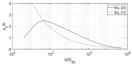
Figure 1. Comparison between the Florida Department of Transportation (FDOT) equation and the Colorado State University (CSU) equation.

To generate Figure 1, $V_o$ was assumed to be 1 m/s, $y_o$ was assumed to be 10 m, and $D_{50}$ was assumed to be 1 mm. Guo [20] approximated the Shields [19] diagram using the following set of equations:

$$d_{*}=\frac{\left(s-1\right)g{D}_{50}}{{\nu }^2}$$

(6)

$${\mathsf{\Theta }}_c=\frac{0.23}{d_{*}}+0.054\left(1-\exp \left(-\frac{d_{*}^{0.85}}{23}\right)\right)$$

(7)

$${\tau }_c={\mathsf{\Theta }}_c\left(s-1\right)g{D}_{50}$$

(8)

where s is the sediment’s specific gravity defined by $\frac{{\rho }_s}{\rho }$, $\rho$ is the density of water, ${\rho }_s$ is the sediment’s density, ${\mathsf{\Theta }}_c$ is the shield parameter, ${\tau }_c$ is the critical shear stress corresponding to $V_c$, and $\nu$ is the kinematic viscosity of water. These expressions were used to estimate ${\tau }_c$ for the 1 mm sediment by assuming ${\rho }_s=$ 2500 kg/m³. Then, ${\tau }_c$ was converted to $V_c$ by assuming ${\tau }_c$ corresponded to the Reynolds stress:

$${\tau }_c=\rho u_{*c}^2$$

(9)

Finally, ${\tau }_c$ was converted to $V_c$ using the following expression from HEC-18 [1]:

$$V_c=5.75u_{*c}{\log }_{10}\left(\frac{5.53y_o}{D_{50}}\right)$$

(10)

As shown in Figure 1, both the FDOT and HEC-18 expressions for computing local scour depth behave similarly for increasing values of b in the sense that each “tails off” for higher values of $\frac{b}{D_{50}}$. However, the HEC-18 expression misses the local scour local maximum predicted by the FDOT equation when $\frac{b}{D_{50}}~45$.

2.2. The Texas A&M Formulation

As noted above, at first glance, analysis of Equation (3) does not appear to show much (if any) dependence between scour depth and the $\frac{b}{D_{50}}$ ratio. However, both Froude Numbers in Equation (3) (Equations (4) and (5)) take b into account, and the pier Froude Number (Equation (4)) takes grain size information into account indirectly in the sense that $V_c$ is known to be a function of $D_{50}$ and ${\rho }_s$. Using the Shields [19] approximation in Equation (6) through Equation (8), values for ${\tau }_c$ were computed for several $D_{50}$ values and converted to $V_c$ using Equation (9) and Equation (10) by assuming ${\rho }_s=$ 2500 kg/m³. Then, assuming $V_o$ = 1 m/s and $y_o=$ 10 m, two sets of computations were conducted using Equation (3). First, b was varied while $D_{50}$ was fixed at 1 mm, and then $D_{50}$ was varied while b was fixed at 1 m. Results of this computation are shown in Figure 2.

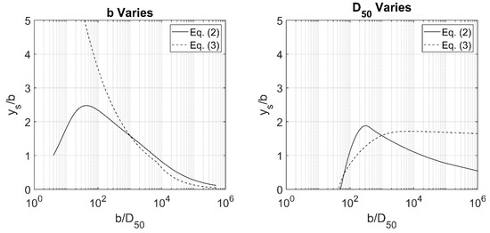
Figure 2. Predicted equilibrium scour depth using the FDOT and Oh [18] formulations.

As shown, the FDOT equations respond relatively similarly when b or $D_{50}$ are varied. Their slight differences are attributed to the additional $\frac{V}{V_c}$ dependency that is considered in Equation (2). On the other hand, the Oh [18] formulation responds very differently if b or $D_{50}$ are varied. When b is varied, the Oh [18] formulation behaves similarly to both the FDOT Equation and the CSU Equation for high $\frac{b}{D_{50}}$ values in the sense that predicted $\frac{y_s}{b}$ decreases as a function of $\frac{b}{D_{50}}$. However, like the CSU Equation, varying b and using the Oh [18] formulation predict significantly higher $\frac{y_s}{b}$ values for low $\frac{b}{D_{50}}$ ratios. On the other hand, when $D_{50}$ varies, the Oh [18] formulation performs similarly to the FDOT Equation in the sense that increases in $\frac{b}{D_{50}}$ lead to increases in predicted $\frac{y_s}{b}$. As such, a pseudo-peak like the peak predicted by the FDOT equations is realized. However, unlike the FDOT Equation, the Oh [18] formulation fails to “tail off” for high $\frac{b}{D_{50}}$ values when b is varied. Taken holistically, it would appear that the Oh [18] formulation is taking the $\frac{b}{D_{50}}$ ratio into account indirectly to some extent. However, it fails to take the $\frac{b}{D_{50}}$ ratio into account explicitly, and as such, the formulation does not exactly replicate the FDOT formulation behavior for all values of $\frac{b}{D_{50}}$.

2.3. Sheppard’s b/D₅₀ Dependency Due to Potential Flow Theory

The following follows Sheppard [16] whereby potential flow theory was used to justify the apparent dependency between $y_s$ and $\frac{D_{50}}{b}$. The stream function for flow around a circular cylinder may be written in polar coordinates as:

$$\psi =V_0\sin \left\{\theta \left[1-{\left(\frac{a}{r}\right)}^2\right]\right\}$$

(11)

where $\psi$ is the stream function, $V_0$ is the depth mean velocity of the approach flow, r is the radial coordinate, $\theta$ is the angular coordinate, and a is the radius of the circular pile (i.e., $\frac{b}{2}$). The radial and angular components of velocity in terms of the stream function are then:

$$V_r=\frac{1}{r}\frac{\partial \psi }{\partial \theta }=V_0\cos \left\{\theta \left[1-{\left(\frac{a}{r}\right)}^2\right]\right\}$$

(12)

$$V_{\theta }=\frac{\partial \psi }{\partial r}=-V_0\sin \left\{\theta \left[1+{\left(\frac{a}{r}\right)}^2\right]\right\}$$

(13)

where $V_r$ is the radial velocity component and $V_{\theta }$ is the angular velocity component. The magnitude of velocity is then:

$$v=\sqrt{V_r^2+V_{\theta }^2}=V_0\sqrt{{\left(\frac{a}{r}\right)}^4-2{\left(\frac{a}{r}\right)}^2\cos \left(2\theta \right)+1}$$

(14)

Next, Bernoulli’s equation may be used to express pressure at any point in the flow field. As shown by Sheppard [16]:

$$\frac{2\left(p-p_0\right)}{\rho V_0^2}=1-{\left(\frac{V}{V_0}\right)}^2$$

(15)

in which $p_0$ is the pressure at mid-elevation of the approach flow. Equations (14) and (15) may be nondimensionalized using $U=\frac{V}{V_o}$, $R=\frac{r}{a}$, and $p=\frac{2\left(p-p_o\right)}{\rho V_o^2}$. Substituting and rearranging results in:

$$U=\sqrt{{\left(\frac{1}{R}\right)}^4-2{\left(\frac{1}{R}\right)}^2\cos \left(2\theta \right)+1}$$

(16)

$$p=-{\left(\frac{1}{R}\right)}^2\left[{\left(\frac{1}{R}\right)}^2-2\cos \left(2\theta \right)\right]$$

(17)

Next, the pressure gradient ($\nabla P$) is defined as a vector with a magnitude equal to the maximum spatial change in pressure and a direction defined by that maximum change:

$$\nabla P=\frac{\partial P}{\partial R}{\widehat{e}}_r+\frac{1}{R}\frac{\partial P}{\partial \theta }{\widehat{e}}_{\theta }$$

(18)

in which ${\widehat{e}}_r$ and ${\widehat{e}}_{\theta }$ are unit vectors in the radial and angular directions, respectively. Applying Equation (18) to Equation (17) yields:

$$\nabla P=\left\{4{\left(\frac{1}{R}\right)}^3\left[{\left(\frac{1}{R}\right)}^2-\cos \left(2\theta \right)\right]\right\}{\widehat{e}}_r+\left[8{\left(\frac{1}{R}\right)}^3\sin \left(\theta \right)\cos \left(\theta \right)\right]{\widehat{e}}_{\theta }$$

(19)

The magnitude of the pressure gradient at any point in the flow field is then:

$$\left|\nabla P\right|=\frac{dP}{dN}=4{\left(\frac{1}{R}\right)}^3\sqrt{{\left(\frac{1}{R}\right)}^4-2{\left(\frac{1}{R}\right)}^2\cos \left(2\theta \right)+1}$$

(20)

where N is defined as $n/a$, or the normalized coordinate in the direction of the maximum change of pressure in which n is the dimensional coordinate in the direction of the maximum change of pressure.

Now, the forces acting on a sediment particle at the surface of the bed in the vicinity of the pile must be examined. The magnitude of the drag force ($F_D$) upon this particle is:

$$F_D=\frac{1}{2}{C}_D\rho A{u}^2$$

(21)

where $C_D$ is the drag coefficient, A is the projected area of the particle, and u is the approach velocity at the level of the particle. For the case of a spherical particle, A may be defined as $\pi c^2$, where c is half the particle diameter (D₅₀/2). The force on the particle due to the pressure gradient ($F_p$) may be expressed in differential form as:

$$F_p=-\left(p+\frac{\partial p}{\partial n}c\cos \beta \right)dA$$

(22)

where $\beta$ is the angular coordinate measured from the positive n-direction (positive counterclockwise) and:

$$dA=2\pi \left(c\sin \beta \right)c d\beta =\left(2\pi c^2\sin \beta \right)d\beta$$

(23)

The component of this force in the n-direction ($F_{p\left(n\right)}$) is then:

$$F_{p\left(n\right)}=d{F}_p\cos \beta$$

(24)

After some algebra, integrating the component of the pressure force in the n-direction over the particle surface results in:

$$F_{p\left(n\right)}=-\frac{8\pi c^3\rho V_0^2}{3a}{\left(\frac{1}{R}\right)}^3\sqrt{{\left(\frac{1}{R}\right)}^4-2{\left(\frac{1}{R}\right)}^2\cos \left(2\theta \right)+1}$$

(25)

To find the relative magnitudes of the force on the particle due to the structure-imposed pressure gradient by the force on the particle, $F_{p\left(n\right)}$ must be divided by $F_D$. Dividing Equation (25) by Equation (21) yields (after further algebraic manipulation):

$$\frac{\left|F_{p\left(n\right)}\right|}{\left|F_D\right|}=\frac{16}{3}\left(\frac{1}{C_D}\right)\left(\frac{D_{50}}{b}\right){\left(\frac{V_0}{u}\right)}^2{\left(\frac{1}{R}\right)}^3\sqrt{{\left(\frac{1}{R}\right)}^4-2{\left(\frac{1}{R}\right)}^2\cos \left(2\theta \right)+1}$$

(26)

Note the dependency-term between D₅₀ and b. One can easily plot contours of Equation (26) for various values of $\frac{b}{D_{50}}$ as shown below in Figure 3 and Figure 4:

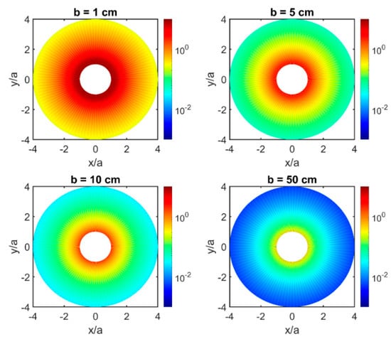
Figure 3. Contours of Equation (26) for increasing values of b assuming $D_{50}$ = 1 mm and $V_0=1$ m/s.

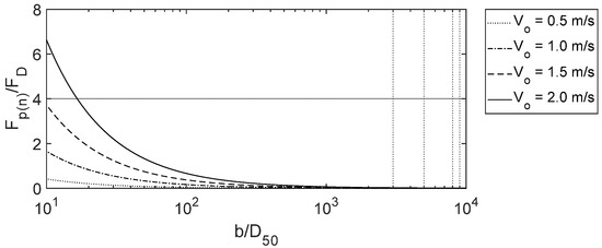
Figure 4. Cross-section through Equation (26) assuming $\theta =0$ and R = 2 for various values of $V_o$.

To generate Figure 3 and Figure 4, $u_{*c}$ was computed using Equation (6) through Equation (9). Then, a log-law was applied:

$$\frac{u}{u_{*c}}=\kappa {\log }_{10}\left(\frac{y}{y_o}\right)$$

(27)

in which $\kappa$ is von Karmann’s constant (i.e., 0.4); y was assumed to be $\frac{D_{50}}{2}$; and $y_o$ was assumed to be $\frac{k_s}{30}$ where $k_s$ denotes the roughness height. Crowley, et al. [21] showed that $k_s$ may be approximated from $D_{50}$ via the relationship $k_s~0.76D_{50}$. $C_D$ was computed as a function of the wall roughness number $R{e}_{*}$ defined by:

$$R{e}_{*}=\frac{u_{*}{D}_{50}}{\nu }$$

(28)

$$C_D=\frac{24}{R{e}_{*}}$$

(29)

As shown in Figure 3 and Figure 4, increases in pile sizes for a given particle size decrease the ratio between pressure gradient force and drag force exponentially. The shape of the curves shown in Figure 4 is similar to the shape captured by the CSU Equation, the FDOT Equation, and the Oh [18] equation with varied b in the sense that the ratio between pressure gradient force and drag force on bed particles “tails off” as the $\frac{b}{D_{50}}$ ratio increases. This implies that as structure size increases relative to grain size, scour depth too should show a similar decrease when examined as a function of the $\frac{b}{D_{50}}$ ratio. Put another way, this derivation appears to give further credibility to the dependence between local scour and the $\frac{b}{D_{50}}$ ratio.

2.4. A New b/D₅₀ Explanation Based Upon Turbulence

A similar $\frac{b}{D_{50}}$ dependency may be derived using a turbulent energy spectrum decay. Assume the following:

• The presence of the pile initiates turbulent eddies at a distance scale, L.
• Turbulence obeys Kolmogorov scaling in the sense that energy cascades from large to small scales and energy dissipated at small scales is replenished by larger-scale eddies.
• Dissipation occurs at a scale $D_{50}$ set by the sediment.
• Energy is lost from the moving water when sediment is lifted and accelerated to $V_o$ on a time scale set by the diffusion time at the scale of the sediment.

Consider a cube of water with dimension L centered around a pile. Assume this cube is moving with the water and that the dimension $L\left(y\right)$ represents the largest eddy structures that are allowed to diminish as a function of y, where y is the varying water depth during the scour process. Due to Kolmogorov scaling, the energy spectrum in this cube is initially:

$$E\left(k\right)=\alpha {ϵ}^{\frac{2}{3}}{k}^{-\frac{5}{3}}$$

(30)

where $ϵ$ is the turbulent dissipation rate and $\alpha$ is Kolmogorov’s constant, which is usually assumed to be 1.62. The total energy within the box at position y is then:

$$E\left(y\right)={{\displaystyle \int }}_{k_{min}}^{k_{max}}E\left(k\right)dk$$

(31)

Due to assumption 3, $k_{max}$ is approximately $\frac{2\pi }{D_{50}}$. This is small relative to $k_{min}$, which is given by $k_{min}=\frac{2\pi }{L\left(y\right)}$. Performing the integral from Equation (31):

$$E\left(y\right)=\frac{2}{3}\alpha {ϵ}^{\frac{2}{3}}{\left(\frac{L}{2\pi }\right)}^{\frac{2}{3}}$$

(32)

Due to conservation of energy, $\frac{\partial E\left(y\right)}{\partial t}=v\frac{\partial E\left(y\right)}{\partial y}=-ϵ$. The energy lost by the water must be absorbed by the sediment. Therefore, the change in the sediment’s energy must be found. The sediment goes from zero energy to an energy of $\frac{m{v}^2}{2}$ in a time $\mathsf{∆}t$, where m is the mass of a sediment layer which may be estimated as $m={\rho }_s{L}^2{D}_{50}$.

Next, define $\mathsf{∆}t$ as the diffusion time at this distance scale, which may be approximated by $\mathsf{∆}t=\frac{D_{50}^2}{\mu }$ in which $\mu$ is turbulent diffusivity. Writing $ϵ=\sigma L^2$ where $\sigma =\frac{{\rho }_s{V}_o^2{D}_{50}}{2\mathsf{∆}t}$, conservation of energy may be expressed as:

$$v\frac{d}{dx}\left(\frac{2}{3{\left(2\pi \right)}^{\frac{2}{3}}} \alpha {\sigma }^{\frac{2}{3}} L^2\left(y\right)\right)=-\sigma L^2$$

(33)

Solving for $L\left(y\right)$:

$$L\left(y\right)=L\exp \left(-\frac{3{\left(2\pi \right)}^{\frac{2}{3}}{\sigma }^{\frac{1}{3}}}{4 \alpha V_o}\right)$$

(34)

This process must end when $L=D_{50}$. Solving for the value of y when this happens gives an expression for post-scour water depth:

$$y_s=\frac{4\alpha V_o}{3{\left(2\pi \right)}^{\frac{2}{3}}{\sigma }^{\frac{1}{3}}}\ln \left(\frac{L}{D_{50}}\right)$$

(35)

A bit of algebra leads to the following:

$$y_s=\frac{2^{\frac{1}{3}}4\alpha }{3{\left(2\pi \right)}^{\frac{2}{3}}} {\left(V_o\frac{D_{50}}{\mu {\rho }_s}\right)}^{\frac{1}{3}}\ln \left(\frac{L}{D_{50}}\right)$$

(36)

Finally, assuming the cube of water defined by L is limited by structure size, b:

$$y_s=\frac{2^{\frac{1}{3}}4\alpha }{3{\left(2\pi \right)}^{\frac{2}{3}}} {\left(\frac{V_o{D}_{50}}{\mu {\rho }_s}\right)}^{\frac{1}{3}}\ln \left(\frac{b}{D_{50}}\right)$$

(37)

Again, note the dependency between scour depth and ratio between structure and grain size. Additionally, note that dependency between scour depth and $V_o^{\frac{1}{3}},$ which is relatively close to the $V_o^{0.43}$ dependency shown in the CSU Equation. While these are positive, the downside to Equation (37) is that the scour problem has been transformed into a problem where turbulent diffusivity must be solved. For the purposes of this paper, $\mu$ was assumed to be equal to $5\times {10}^{-5}$ m²/s simply because this value for $\mu$ appeared to replicate the shape predicted by the FDOT equations when examined in the context of $\frac{b}{D_{50}}$. However, in future work, this can easily be improved upon by calibrating $\mu$ using existing data from the literature or boundary layer statistics. Plots of Equation (37) as a function of $\frac{b}{D_{50}}$ are presented for varying b and $D_{50}$ in Figure 5 using the same values for V, $y_o$, etc. discussed in the previous example problems.

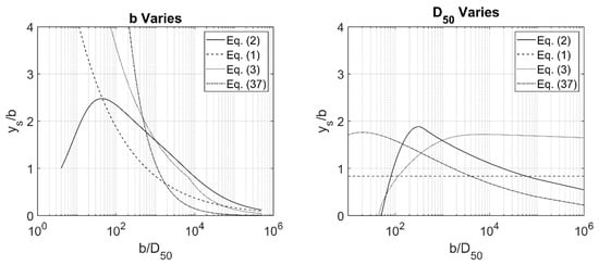
Figure 5. Plots of Equation (37) for various $V_o$ values.

As shown, when b is varied in Equation (37), predicted $y_s$ behaves similarly to both the CSU Equation and the Oh [18] formulation. Unlike the FDOT Equation, Equation (37) does not predict a peak $y_s$ value when b is varied. However, when $D_{50}$ is varied, Equation (37) produced a peak value for $y_s$ that is very similar to the FDOT expression except the peak is produced at a lower $\frac{b}{D_{50}}$ value. Similarly, like the FDOT expression, Equation (37) “tails off” as a function of $\frac{b}{D_{50}}$ for decreasing values of b. This contrasts as well with the CSU expression in the sense that changing b with the CSU equation has no effect on predicted values for $y_s$.

Overall, the shape of Equation (37) is promising. If the $\mu$ issue can be resolved, it is possible that these noted deficiencies (at least compared with the FDOT Equation, which is considered the “gold standard”) associated with Equation (37) may be resolved. If so, this could represent a new, physically-based method for predicting equilibrium scour depth in the future. Even without this, however, Equation (37)′s response to $\frac{b}{D_{50}}$ is similar to previous equations’ responses, and it represents another physical reason for the apparent dependency between equilibrium scour depth and the $\frac{b}{D_{50}}$ ratio.

3. Discussion, Summary, and Conclusions

To summarize:

• This paper presented a review of steady flow local scour dependency on the ratio between structure size and grain size. As noted in this manuscript, the current state-of-the-art empirical formulations for steady flow equilibrium scour depth appear to take this ratio into account to some extent. The formulation from FDOT takes the ratio into account directly, while the formulation from the Briaud group takes the ratio into account indirectly. The CSU equation appears to miss the dependency because $D_{50}$ is not taken into account.
• Work from Sheppard [16] gave an apparent reason for the dependency between the structure/grain size ratio and equilibrium scour depth. As Sheppard [16] showed, flow around a pile causes a pressure gradient. However, flow around the soil particles themselves also causes smaller pressure gradients around the particles. The superposition of these two pressure gradients leads to the dependency between scour depth and the grain size/structure size ratio.
• This paper also presented a possible new explanation for the dependency between equilibrium scour depth and the structure/grain size ratio using a turbulent energy spectrum decay argument. This formulation was similar to the well-known CSU equation in the sense that in addition to the dependency between equilibrium scour depth and $\frac{b}{D_{50}}$, equilibrium scour depth also appears to be a function of the local velocity.

Overall, the analysis presented here shows several pieces of evidence that suggest that steady flow local equilibrium scour depth should be dependent upon the ratio between structure size and grain size. The advantage to the new energy decay model is that it is a physically-based method for predicting local equilibrium scour depth that appears to take well-known nondimensional numbers into account the local Reynolds Number and the $\frac{b}{D_{50}}$ ratio. In a sense, this new turbulent-based model for describing scour is similar to the work presented by Sheppard [16]. The Sheppard [16] explanation’s physical meaning is that flow in the presence of a bridge pier creates a pressure gradient around the pier. Similarly, flow past a soil particle will result in its own pressure gradient. The superposition of these two pressure gradients causes the $\frac{b}{D_{50}}$ dependency. Equation (37) was derived assuming that a pier will cause turbulence whose eddies are similar in scale to the size of the pier. Turbulent energy will then cascade until it reaches the particle-scale. This cascade of energy from the pile’s turbulence-scale to the particle’s turbulence scale causes the $\frac{b}{D_{50}}$ local scour dependency. In other words, the turbulence associated with the flow around the particle is interacting with the turbulence created by flow around the pier. In both cases, the production of turbulence implies the formation of pressure gradients. This is essentially the same argument presented by Sheppard [16], just viewed from a different lens.

Of course, the disadvantage to Equation (37) is that using this model would require a better overall understanding of turbulent diffusivity, a complicated topic that is in and of itself its own extensive field of research! In future work, this could likely be refined/improved upon by paying closer attention to other mechanisms for energy dissipation at smaller values of $\frac{b}{D_{50}}$. It may even be possible to recreate the local maximum predicted by the FDOT equations by noting that as b approaches zero, energy will transfer to heat and not cause the natural logarithm predicted by Equation (37) to approach negative infinity. Future work will be aimed at better approximating this phenomenon as well as calibrating the diffusivity coefficient using existing experimental data.

References

- Arneson, L.A.; Zevenburgen, L.W.; Lagasse, P.F.; Clopper, P.E. Evaluating Scour at Bridges, 5th ed.; Federal Highway Administration: Washington, DC, USA, 2012.
- Laursen, E.M. Scour at Bridge Crossings. J. Hydraul. Div. 1960, 86, 39–54. [Google Scholar]
- Jain, S.C.; Fischer, R.E. Scour Around Bridge Piers at High Froude Numbers; Federal Highway Administration, US Department of Transportation: Washington, DC, USA, 1979.
- Laursen, E.M. Predicting Scour at Bridge Piers and Abutments; Arizona Department of Transportation: Phoenix, AZ, USA, 1980.
- Richardson, E.V.; Simons, D.B.; Lagasse, P.F. River Engineering for Highway Encroachments—Highways in the River Environment; Federal Highway Administration: Washington, DC, USA, 2001.
- Melville, B.W.; Sutherland, A.J. Design Method for Local Scour at Bridge Piers. J. Hydraul. Eng. 1988, 114, 1210–1226. [Google Scholar] [CrossRef]
- Jones, J.S. Comparison of prediction equations for bridge pier and abutment scour. In Proceedings of the Transportation Research Record 950, Second Bridge Engineering Conference, Washington, DC, USA, 24–26 September 1984. [Google Scholar]
- Mueller, D.S. Local Scour at Bridge Piers in Nonuniform Sediment under Dymamic Conditions; Colorado State University: Fort Collins, CO, USA, 1996. [Google Scholar]
- Landers, M.N.; Mueller, D.S.; Richardson, E.V. U.S. Geological Survey Field Measurements of Pier Scour; Lagasse, R.A., Ed.; ASCE: Reston, VA, USA, 1999. [Google Scholar]
- FDOT. FDOT Bridge Scour Manual; Florida Department of Transportation: Tallahassee, FL, USA, 2005.
- Ettema, R. Scour at Bridges; University of Auckland, School of Engineering: Auckland, New Zealand, 1980. [Google Scholar]
- Froehlich, D.C. Analysis of on-site scour at Bridge Piers. In Proceedings of the Hydraulic Engineering Conference, Colorado Springs, CO, USA, 8–12 August 1988. [Google Scholar]
- Garde, R.J.; Ranga Raju, K.G.; Kothyari, U.C. Effect of Unsteadiness and Stratification on Local Scour; International Science Publisher: New York, NY, USA, 1993. [Google Scholar]
- Sheppard, D.M.; Zhao, G.; Ontowirjo, B. Local scour near single piles in steady currents. In Proceedings of the 1st International Conference on Water Resources Engineering, San Antonio, TX, USA, 14–18 August 1995; pp. 1809–1813. [Google Scholar]
- Sheppard, D.M.; Odeh, M.; Glasser, T. Large Scale Clear-Water Local Pier Scour Experiments. J. Hydraul. Eng. 2004, 130, 957–963. [Google Scholar] [CrossRef]
- Sheppard, D.M. An Overlooked Local Sediment Scour Mechanism. Transp. Res. Rec. 2004, 1890, 107–111. [Google Scholar] [CrossRef]
- Sheppard, D.M.; Miller, W. Live-Bed Local Pier Scour Experiments. J. Hydraul. Eng. 2006, 132, 635–642. [Google Scholar] [CrossRef]
- Oh, S.J. Experimental Study of Bridge Scour in Cohesive Soil. Ph.D. Thesis, Texas A&M University, College Station, TX, USA, December 2009. [Google Scholar]
- Shields, A.F. Application of Similarly Principles and Turbulence Research to Bed-Load Movement; CalTech: Pasadena, CA, USA, 1936. [Google Scholar]
- Guo, J.J.; Guo, J. Hunter rouse and shields diagram. In Advances in Hydraulics and Water Engineering; World Scientific Pub Co Pte Lt: Singapore, 2002; pp. 1096–1098. [Google Scholar]
- Crowley, R.W.; Bloomquist, D.; Hayne, J.R.; Holst, C.M.; Shah, F.D. Estimation and Measurement of Bed Material Shear Stresses in Erosion Rate Testing Devices. J. Hydraul. Eng. 2012, 138, 990–994. [Google Scholar] [CrossRef]
Publisher’s Note: MDPI stays neutral with regard to jurisdictional claims in published maps and institutional affiliations. |
© 2020 by the authors. Licensee MDPI, Basel, Switzerland. This article is an open access article distributed under the terms and conditions of the Creative Commons Attribution (CC BY) license (http://creativecommons.org/licenses/by/4.0/).