Internal Wave Generation in a Non-Hydrostatic Wave Model

Abstract

In this work, internal wave generation techniques are developed in an open source non-hydrostatic wave model (Simulating WAves till SHore, SWASH) for accurate generation of regular and irregular long-crested waves. Two different internal wave generation techniques are examined: a source term addition method where additional surface elevation is added to the calculated surface elevation in a specific location in the domain and a spatially distributed source function where a spatially distributed mass is added in the continuity equation. These internal wave generation techniques in combination with numerical wave absorbing sponge layers are proposed as an alternative to the weakly reflective wave generation boundary to avoid re-reflections in case of dispersive and directional waves. The implemented techniques are validated against analytical solutions and experimental data including water surface elevations, orbital velocities, frequency spectra and wave heights. The numerical results show a very good agreement with the analytical solution and the experimental data indicating that SWASH with the addition of the proposed internal wave generation technique can be used to study coastal areas and wave energy converter (WEC) farms even under highly dispersive and directional waves without any spurious reflection from the wave generator.

1. Introduction

Numerical wave propagation models are commonly used as engineering tools for the study of wave transformation in coastal areas. The number of numerical models based on the Navier-Stokes equation has recently increased remarkably, since they offer detailed and accurate predictions of the wave field but at a very high computational cost. As a result, numerical models solving approximated equations usually averaged over the vertical—like Boussinesq and nonlinear shallow water equations—are an essential tool, especially when large domains and sea states of several hours are considered.

Boussinesq-type models [1,2,3] account for both nonlinearity and frequency-dispersion of the waves by using high-order derivative terms in the equations. As an alternative, models based on the non-hydrostatic approach [4,5,6] can resolve the vertical flow structure and can improve their frequency dispersion by using additional layers rather than increasing the order of derivatives as in the case of Boussinesq-type models. A representative model of this latter category is SWASH [7], a phase-resolving wave propagation model based on the nonlinear shallow water equations with added non-hydrostatic effects. In the field of wave transformation in coastal areas, SWASH has already reached a fairly mature stage since it can incorporate nonlinear shallow-water effects, such as the generation of bound sub- and super-harmonics and near-resonant triad interactions [8,9,10,11].

In order to simulate waves in the nearshore zone correctly, the generation and absorption of waves at the boundary of models need to be modelled accurately. In the SWASH model, incident waves are generated by prescribing their horizontal velocity component normal to the boundary of the computational domain over the vertical direction. Additionally, to absorb and to prevent re-reflections in front of the numerical wave generator, a weakly reflective wave generation boundary condition [12] is applied in which the total velocity signal is a superposition of the incident velocity signal and a velocity signal of the reflected waves [13]. Verbrugghe et al. [14] applied a similar method to create open boundaries within a Smoothed Particle Hydrodynamics (SPH) solver. However, this method is based on the assumption that the reflected waves are small amplitude shallow water waves propagating perpendicular to the boundary of the computational domain and hence this method is weakly reflective for directional, dispersive waves. Furthermore, Wei and Kirby [15] found that this type of radiation condition at the wave generator boundary can lead to numerical errors when long time simulations are performed. Recently, a generating absorbing boundary condition (GABC) has been developed which is an enhanced type of a weakly reflective wave generation boundary condition and can partially absorb dispersive and directional waves [16,17]. However, in this method the level of re-reflection strongly depends on the initial approximations since the characteristics of the reflected waves (i.e., wave angle, wave celerity) inside the numerical domain cannot be estimated a priori. In general, it is not possible to find practical boundary conditions that do the above task perfectly.

On the other hand, models utilizing a sponge layer are very effective in absorbing reflected waves. However, this implies that the waves have to be generated inside the computational domain instead of on the boundary. This internal wave generation technique in combination with numerical wave absorbing sponge layers was firstly proposed by Larsen and Dancy [18] for Peregrine’s classical Boussinesq equations [19]. Later, Lee and Suh [20] and Lee et al. [21] achieved wave generation for the mild slope equations of Reference [22] and the extended Boussinesq equations of Nwogu [23], respectively, by applying the source term addition method. Lee et al. [21] have shown empirically that the velocity of disturbances caused by the incident wave can be properly obtained from the viewpoint of energy transport. Further, Schäffer and Sørensen [24] theoretically derived the energy velocity by adding the delta source function to the mass conservation type equation and integrated asymptotically the resulting equation at the generation point. However, Wei et al. [25] found that the source term addition method in a single source line may cause high frequency noise in case of non-staggered computational grid. To deal with this problem, Wei et al. [25] derived a spatially distributed (Gaussian shape) source function for internal wave generation, where a mass source is added in the continuity equation. Later, Choi and Yoon [26] and Ha et al. [27] used this technique in a Reynolds-averaged Navier-Stokes (RANS) equations model and a Navier-Stokes equations (NSE) model, respectively. However, in both cases they used directly the formula of [25], which was derived from the Boussinesq equations under the shallow water assumption. Thus, their model was not capable to accurately generating deep water waves and consequently high-frequency components in case of irregular waves.

In the present paper, a source term addition method and a spatially distributed source function for internal wave generation are implemented in the non-hydrostatic model SWASH, in order accurately generate regular and irregular long-crested waves. In addition, the energy velocity will be derived for the governing equations of SWASH in case multiple layers are implemented. To the present authors’ knowledge, these internal wave generation techniques which are commonly used in Boussinesq models [3] and mild-slope wave models [28], have not been derived and used in a non-hydrostatic wave model before, due to the complexity of the governing equations. So, the main objective of the present work concerns the implementation of the internal wave generation in SWASH to accurately generate even highly dispersive and directional waves, while at the same time re-reflections at the position of the wave generator are vanishing. Moreover, SWASH has already been used in the field of marine energy by simulating the wave-induced response of a submerged wave-energy converter [29]. This kind of application requires a homogeneous wave field in the whole numerical domain. Thus, the implementation of internal wave generation is important as it introduces noteworthy improvements in the model, which can then make full use of its benefits for the study of WEC farms.

The paper is structured as follows. The numerical model SWASH is described in Section 2 where the governing equations are presented. The implemented internal wave generation techniques are derived in Section 3. Section 4 provides a detailed overview of the model results for regular and irregular long-crested waves. In addition, validation results are presented where the accuracy of the model is compared with experimental data. The last sections provide conclusions and a summary discussion of the present study.

2. SWASH Model

2.1. Mathematical Formulation

SWASH is an open source non-hydrostatic wave model [7]. The governing equations of the model are based on the nonlinear shallow water equations with added non-hydrostatic effects, which are derived from the incompressible Navier-Stokes equations. The numerical domain is bounded vertically by the free-surface $\mathrm{z}=\mathsf{\eta }\left(\mathrm{x},\mathrm{t}\right)$ and the bottom $\mathrm{z}=-\mathrm{d}\left(\mathrm{x}\right)$, where $\mathrm{t}$ is time, $\mathrm{d}$ is the still water depth and $\mathrm{x}$ and $\mathrm{z}$ are the Cartesian coordinates, where z is directed positive upwards. The equations for the 2D vertical domain are

$$\frac{\partial \mathrm{u}}{\partial \mathrm{x}}+\frac{\partial \mathrm{w}}{\partial \mathrm{z}}=0$$

(1)

$$\frac{\partial \mathrm{u}}{\partial \mathrm{t}}+\frac{\partial \mathrm{uu}}{\partial \mathrm{x}}+\frac{\partial \mathrm{wu}}{\partial \mathrm{z}}=-\frac{1}{{\mathsf{\rho }}_0}\frac{\partial \left({\mathrm{p}}_{\mathrm{h}}+{\mathrm{p}}_{\mathrm{nh}}\right)}{\partial \mathrm{x}}+\frac{\partial {\mathsf{\tau }}_{\mathrm{xz}}}{\partial \mathrm{z}}+\frac{\partial {\mathsf{\tau }}_{\mathrm{xx}}}{\partial \mathrm{x}}$$

(2)

$$\frac{\partial \mathrm{w}}{\partial \mathrm{t}}+\frac{\partial \mathrm{uw}}{\partial \mathrm{x}}+\frac{\partial \mathrm{ww}}{\partial \mathrm{z}}=-\frac{1}{{\mathsf{\rho }}_0}\frac{\partial {\mathrm{p}}_{\mathrm{nh}}}{\partial \mathrm{z}}+\frac{\partial {\mathsf{\tau }}_{\mathrm{zz}}}{\partial \mathrm{z}}+\frac{\partial {\mathsf{\tau }}_{\mathrm{zx}}}{\partial \mathrm{x}}$$

(3)

where $\mathrm{u}\left(\mathrm{x},\mathrm{z},\mathrm{t}\right)$ and $\mathrm{w}\left(\mathrm{x},\mathrm{z},\mathrm{t}\right)$ are the horizontal and vertical velocities, ${\mathrm{p}}_{\mathrm{h}}$ and ${\mathrm{p}}_{\mathrm{nh}}$ are the hydrostatic and non-hydrostatic pressures, ${\mathsf{\rho }}_0$ is density and ${\mathsf{\tau }}_{\mathrm{xx}}$, ${\mathsf{\tau }}_{\mathrm{xz}}$, ${\mathsf{\tau }}_{\mathrm{zx}}$, ${\mathsf{\tau }}_{\mathrm{zz}}$ are the turbulent stresses. The kinematic boundary conditions are

$$\mathrm{w}=\frac{\partial \mathsf{\eta }}{\partial \mathrm{t}}+\mathrm{u}\frac{\partial \mathsf{\eta }}{\partial \mathrm{x}}\left(\mathrm{z}=\mathsf{\eta }\right)$$

(4)

$$\mathrm{w}=-\mathrm{u}\frac{\partial \mathrm{d}}{\partial \mathrm{x}}\left(\mathrm{z}=-\mathrm{d}\right)$$

(5)

The dynamic boundary conditions at the surface are a constant pressure and no surface stresses. The free surface elevation $\mathsf{\eta }$ is determined by considering the continuity for the entire water column

$$\frac{\partial \mathsf{\eta }}{\partial \mathrm{t}}+\frac{\partial }{\partial \mathrm{x}}{{\displaystyle \int }}_{-\mathrm{d}}^{\mathsf{\eta }}\mathrm{udz}=0$$

(6)

At the bottom boundary, a bottom stress is included based on a quadratic friction law

$${\mathsf{\tau }}_{\mathrm{b}}={\mathrm{c}}_{\mathrm{f}}\frac{\mathrm{U}\left|\mathrm{U}\right|}{\mathrm{h}}$$

(7)

where $\mathrm{h}=\mathsf{\eta }+\mathrm{d}$ is the total water depth, $\mathrm{U}$ is the depth averaged velocity and ${\mathrm{c}}_{\mathrm{f}}$ is a dimensionless friction coefficient.

At the outlet of the domain a sponge layer can be employed to minimize reflections. The sponge layer formula as described in Reference [30] is used, where the free surface elevation $\mathsf{\eta }$ and the velocity component $\mathrm{u}$ are relaxed at every time step.

In SWASH the full process of wave breaking is not simulated but instead a breaking wave is considered analogous with a hydraulic bore. However, a high vertical resolution is needed to resolve accurately this process. Hence, Smit et al. [31] proposed a breaking formulation which can reproduce wave breaking with a coarse vertical resolution. A hydrostatic pressure distribution is assumed when $\partial \mathsf{\eta }/\partial \mathrm{t}>\mathrm{a}\sqrt{\mathrm{gh}}$, where $\mathrm{g}$ is the gravitational acceleration and $\mathrm{a}$ is the maximum wave steepness before breaking.

The numerical implementation is based on an explicit, second order finite difference method for staggered grids, where the mass and momentum are strictly conserved at a discrete level. In the horizontal direction rectilinear or orthogonal curvilinear grid can be applied, while in the vertical direction the computational domain is divided into a fixed number of layers. A more detailed overview of the numerical methods and equations are given in Reference [7].

2.2. Wave Generation in SWASH

In the SWASH model, incident waves are generated by prescribing their horizontal velocity component normal to the boundary of the computational domain over the vertical direction. To prevent re-reflections in front of the numerical wave generator, a weakly reflective wave generation boundary condition is adopted [12]. For the case of one layer the imposed depth-averaged horizontal velocity component is given by

$$\mathrm{u}\left(\mathrm{t}\right)=\frac{\mathsf{\omega }}{\mathrm{kd}}{\mathsf{\eta }}_{\mathrm{t}}+\sqrt{\frac{\mathrm{g}}{\mathrm{d}}}\left({\mathsf{\eta }}_{\mathrm{t}}-{\mathsf{\eta }}_{\mathrm{i}}\right)$$

(8)

where $\mathsf{\omega }$ is the angular frequency, $\mathrm{k}$ is the wave number, $\mathrm{d}$ is the still water depth, $\mathrm{g}$ is the gravitational acceleration, ${\mathsf{\eta }}_{\mathrm{t}}$ is the target surface elevation and ${\mathsf{\eta }}_{\mathrm{i}}$ is the instantaneous surface elevation. In case of multiple layers, a hyperbolic cosine distribution is assumed for the horizontal velocity component. As it can be noticed from the second term of Equation (8), this method is valid only in case that the reflected waves are shallow water waves propagating perpendicular to the boundary of the computational domain, since a shallow water phase velocity, $\mathrm{C}=\sqrt{\mathrm{gd}}$ is used. Hence, it is assumed that the high frequency energy gets dissipated inside the numerical domain before arriving to the wave generation boundary [31]. In addition, a linear superposition of the incident and reflected wave is assumed and thus can only be applied to small amplitude waves.

3. Internal Wave Generation

In cases of directional and dispersive waves an internal wave generation technique can be applied to avoid re-reflections due to the weakly reflective wave generation boundary. Two different internal wave generation techniques are proposed here and are implemented in the SWASH model. The first one is a source term addition method proposed by Lee et al. [21], while the second one is a spatially distributed source function proposed by Wei et al. [25].

3.1. Energy Velocity

At first, a new energy velocity for the system of SWASH equations is mathematically derived following the methodology of Reference [24] who derived the energy velocity for Nwogu’s Boussinesq equations. In this paper, the derivation for the case of two equidistant vertical layers is presented, while the extension to more layers is straightforward.

Bai and Cheung [32] showed that the governing Equations (1)–(3) can be converted into a Boussinesq form by expressing the non-hydrostatic pressure and vertical velocity component in terms of surface elevation and horizontal velocity component. Adding a point source to the continuity equation, the linearized governing equations on a constant depth for the case of two equidistant vertical layers read

$$\frac{\partial \mathsf{\eta }}{\partial \mathrm{t}}+\mathrm{d}\frac{\partial \mathrm{u}}{\partial \mathrm{x}}=\mathsf{\Lambda }\left(\mathrm{t}\right)\mathsf{\delta }\left(\mathrm{x}\right)$$

(9)

$$\frac{\partial \mathrm{u}}{\partial \mathrm{t}}+\mathrm{g}\frac{\partial \mathsf{\eta }}{\partial \mathrm{x}}-\frac{5}{16}{\mathrm{d}}^2\frac{{\partial }^3\mathrm{u}}{\partial {\mathrm{x}}^2\partial \mathrm{t}}-\frac{1}{8}{\mathrm{d}}^2\frac{{\partial }^3\hat{\mathrm{u}}}{\partial {\mathrm{x}}^2\partial \mathrm{t}}=0$$

(10)

$$\frac{\partial \hat{\mathrm{u}}}{\partial \mathrm{t}}-\frac{1}{8}{\mathrm{d}}^2\frac{{\partial }^3\mathrm{u}}{\partial {\mathrm{x}}^2\partial \mathrm{t}}-\frac{1}{16}{\mathrm{d}}^2\frac{{\partial }^3\hat{\mathrm{u}}}{\partial {\mathrm{x}}^2\partial \mathrm{t}}=0$$

(11)

where $\mathrm{u}$ is the depth integrated horizontal velocity component, $\hat{\mathrm{u}}$ is the inter-layer velocity variations, $\mathsf{\delta }$ is the Dirac delta function and $\mathsf{\Lambda }$ is the source function applied to a single point. From Equation (9) it can be noticed that the $\partial \mathrm{u}/\partial \mathrm{x}$ term must be the one balancing the Dirac delta function and thus $\mathrm{u}$ and $\hat{\mathrm{u}}$ have a discontinuity.

Taking the time derivative of Equation (10) and eliminating $\mathsf{\eta }$ from Equation (9) gives

$$\frac{{\partial }^2\mathrm{u}}{\partial {\mathrm{t}}^2}-\mathrm{gd}\frac{{\partial }^2\mathrm{u}}{\partial {\mathrm{x}}^2}-\frac{5}{16}{\mathrm{d}}^2\frac{{\partial }^4\mathrm{u}}{\partial {\mathrm{x}}^2\partial {\mathrm{t}}^2}-\frac{1}{8}{\mathrm{d}}^2\frac{{\partial }^4\hat{\mathrm{u}}}{\partial {\mathrm{x}}^2\partial {\mathrm{t}}^2}=-\mathrm{g}\mathsf{\Lambda }\frac{\partial \mathsf{\delta }}{\partial \mathrm{x}}$$

(12)

Eliminating the second and third term of Equation (12) using Equation (11) to get

$$\frac{{\partial }^2\mathrm{u}}{\partial {\mathrm{t}}^2}-8\frac{\mathrm{g}}{\mathrm{d}}\hat{\mathrm{u}}+\frac{1}{2}\mathrm{gd}\frac{{\partial }^2\hat{\mathrm{u}}}{\partial {\mathrm{x}}^2}-\frac{5}{2}\frac{{\partial }^2\hat{\mathrm{u}}}{\partial {\mathrm{t}}^2}+\frac{1}{32}{\mathrm{d}}^2\frac{{\partial }^4\hat{\mathrm{u}}}{\partial {\mathrm{x}}^2\partial {\mathrm{t}}^2}=-\mathrm{g}\mathsf{\Lambda }\frac{\partial \mathsf{\delta }}{\partial \mathrm{x}}$$

(13)

Taking the x derivative two times and eliminating the first term using Equation (11) gives

$$8\frac{1}{{\mathrm{d}}^2}\frac{{\partial }^2\hat{\mathrm{u}}}{\partial {\mathrm{t}}^2}-8\frac{\mathrm{g}}{\mathrm{d}}\frac{{\partial }^2\hat{\mathrm{u}}}{\partial {\mathrm{x}}^2}+\frac{1}{2}\mathrm{gd}\frac{{\partial }^4\hat{\mathrm{u}}}{\partial {\mathrm{x}}^4}-3\frac{{\partial }^4\hat{\mathrm{u}}}{\partial {\mathrm{x}}^2\partial {\mathrm{t}}^2}+\frac{1}{32}{\mathrm{d}}^2\frac{{\partial }^6\hat{\mathrm{u}}}{\partial {\mathrm{x}}^4\partial {\mathrm{t}}^2}=-\mathrm{g}\mathsf{\Lambda }\frac{{\partial }^3\mathsf{\delta }}{\partial {\mathrm{x}}^3}$$

(14)

Integrating 4 times Equation (14) from $\mathrm{x}=-\mathsf{\epsilon }$ to $\mathrm{x}=+\mathsf{\epsilon }$, with the limit $\mathsf{\epsilon }\to 0$ and requiring the integrals of $\hat{\mathrm{u}}$ to be continuous at $\mathrm{x}=0$, we get

$$\frac{1}{2}\mathrm{gd}\left({\hat{\mathrm{u}}}^{+}-{\hat{\mathrm{u}}}^{-}\right)+\frac{1}{32}{\mathrm{d}}^2\left(\frac{{\partial }^2{\hat{\mathrm{u}}}^{+}}{\partial {\mathrm{t}}^2}-\frac{{\partial }^2{\hat{\mathrm{u}}}^{-}}{\partial {\mathrm{t}}^2}\right)=-\mathrm{g}\mathsf{\Lambda }$$

(15)

In Equation (15), $\hat{\mathrm{u}}$ is an odd function and thus the left and right contributions are identical.

In SWASH an approximation of the exact linear dispersion relation, which depends on the number of vertical layers, is used (see Appendix A). For the case of two equidistant layers it is given by

$${\mathsf{\omega }}^2={\mathrm{gk}}^2\mathrm{d}\frac{1+\frac{1}{16}{\left(\mathrm{kd}\right)}^2}{1+\frac{3}{8}{\left(\mathrm{kd}\right)}^2+\frac{1}{256}{\left(\mathrm{kd}\right)}^4}$$

(16)

In addition, at the wave generation boundary, apart from the progressive waves, evanescent modes are included as well. These evanescent modes are a general characteristic of the Equations (9)–(11). Hence, Equation (16) can be rewritten as

$$\begin{array}{cc}\frac{{\mathsf{\omega }}^2\mathrm{d}}{\mathrm{g}}=\frac{{\mathsf{\omega }}_{\mathrm{e}}^2\mathrm{d}}{\mathrm{g}}\to & {\left(\mathrm{kd}\right)}^2\frac{1+\frac{1}{16}{\left(\mathrm{kd}\right)}^2}{1+\frac{3}{8}{\left(\mathrm{kd}\right)}^2+\frac{1}{256}{\left(\mathrm{kd}\right)}^4}={\left({\mathrm{k}}_{\mathrm{e}}\mathrm{d}\right)}^2\frac{1+\frac{1}{16}{\left({\mathrm{k}}_{\mathrm{e}}\mathrm{d}\right)}^2}{1+\frac{3}{8}{\left({\mathrm{k}}_{\mathrm{e}}\mathrm{d}\right)}^2+\frac{1}{256}{\left({\mathrm{k}}_{\mathrm{e}}\mathrm{d}\right)}^4}\end{array}$$

(17)

where $\mathrm{k}$ and ${\mathrm{k}}_{\mathrm{e}}$ are the wave numbers for progressive waves and evanescent modes, respectively. Equation (17) yields two solutions

$$\begin{array}{cc}{\left({\mathrm{k}}_{\mathrm{e}}\mathrm{d}\right)}^2\to {\left(\mathrm{kd}\right)}^2,& {\left({\mathrm{k}}_{\mathrm{e}}\mathrm{d}\right)}^2\to -\frac{1+\frac{1}{16}{\left(\mathrm{kd}\right)}^2}{\frac{1}{16}+\frac{5}{256}{\left(\mathrm{kd}\right)}^2}\end{array}$$

(18)

Furthermore, away from the source point, x = 0, the solutions of Equations (9)–(11) can be written as

$$\mathsf{\eta }={\mathsf{\eta }}_{\mathrm{p}0}\exp \left[\mathrm{i}\left(\mathsf{\omega }\mathrm{t}-\mathrm{kx}\right)\right]+{\mathsf{\eta }}_{\mathrm{e}0}\exp \left[\mathrm{i}\left(\mathsf{\omega }\mathrm{t}-{\mathrm{k}}_{\mathrm{e}}\mathrm{x}\right)\right]$$

(19)

$$\mathrm{u}={\mathrm{u}}_{\mathrm{p}0}\exp \left[\mathrm{i}\left(\mathsf{\omega }\mathrm{t}-\mathrm{kx}\right)\right]+{\mathrm{u}}_{\mathrm{e}0}\exp \left[\mathrm{i}\left(\mathsf{\omega }\mathrm{t}-{\mathrm{k}}_{\mathrm{e}}\mathrm{x}\right)\right]$$

(20)

$$\hat{\mathrm{u}}={\hat{\mathrm{u}}}_{\mathrm{p}0}\exp \left[\mathrm{i}\left(\mathsf{\omega }\mathrm{t}-\mathrm{kx}\right)\right]+{\hat{\mathrm{u}}}_{\mathrm{e}0}\exp \left[\mathrm{i}\left(\mathsf{\omega }\mathrm{t}-{\mathrm{k}}_{\mathrm{e}}\mathrm{x}\right)\right]$$

(21)

where the subscripts p and e stand for progressive and evanescent modes, respectively. By using Equations (10) and (11), the inter-layer velocity amplitude ${\hat{\mathrm{u}}}_{\mathrm{p}0}$ can be expressed in terms of surface elevation amplitude ${\mathsf{\eta }}_{\mathrm{p}0}$

$${\hat{\mathrm{u}}}_{\mathrm{p}0}=-\frac{1}{8}\frac{\mathrm{gk}}{\mathsf{\omega }}\frac{{\left(\mathrm{kd}\right)}^2}{1+\frac{3}{8}{\left(\mathrm{kd}\right)}^2+\frac{1}{256}{\left(\mathrm{kd}\right)}^4}{\mathsf{\eta }}_{\mathrm{p}0}$$

(22)

In addition, the double integral of $\hat{\mathrm{u}}$ with respect to x gives an odd function and it must vanish at the source point, x = 0 and thus from Equation (21) we can write

$${\hat{\mathrm{u}}}_{\mathrm{e}0}=-\frac{{\mathrm{k}}_{\mathrm{e}}{}^2}{{\mathrm{k}}^2}{\hat{\mathrm{u}}}_{\mathrm{p}0}$$

(23)

Finally, Equation (21) at $\mathrm{x}\to 0^{+}$ is imported in Equation (15) and eventually ${\hat{\mathrm{u}}}_{\mathrm{e}0}$ and ${\hat{\mathrm{u}}}_{\mathrm{p}0}$ are going to be replaced using Equations (22) and (23) respectively. As a result, Equation (15) becomes

$$\mathsf{\Lambda }=2{\mathrm{C}}_{\mathrm{e}}{\mathsf{\eta }}_{\mathrm{p}}$$

(24)

where

$${\mathsf{\eta }}_{\mathrm{p}}={\mathsf{\eta }}_{\mathrm{p}0}\exp \left[\mathrm{i}\mathsf{\omega }\mathrm{t}\right]$$

(25)

$${\mathrm{C}}_{\mathrm{e}}=\frac{1}{8}\frac{\mathrm{gk}}{\mathsf{\omega }}\mathrm{d}\left(\frac{{\left(\mathrm{kd}\right)}^2}{1+\frac{3}{8}{\left(\mathrm{kd}\right)}^2+\frac{1}{256}{\left(\mathrm{kd}\right)}^4}\right)\left(1-\frac{{\mathrm{k}}_{\mathrm{e}}{}^2}{{\mathrm{k}}^2}\right)\left(\frac{1}{2}-\frac{1}{32}\frac{{\mathsf{\omega }}^2\mathrm{d}}{\mathrm{g}}\right)$$

(26)

By eliminating $\mathsf{\omega }$ and ${\mathrm{k}}_{\mathrm{e}}$ using Equations (16) and (18), respectively, it can be noticed that the energy velocity ${\mathrm{C}}_{\mathrm{e}}$ is equal to the group velocity ${\mathrm{C}}_{\mathrm{g}}$ as it can be calculated from the approximated dispersion relation by taking the derivative of $\mathsf{\omega }$ with respect to $\mathrm{k}$

$${\mathrm{C}}_{\mathrm{e}}=\frac{64\sqrt{\mathrm{dg}}(256+32{(\mathrm{kd})}^2+5{(\mathrm{kd})}^4)}{\sqrt{(16+{(\mathrm{kd})}^2){(256+96{(\mathrm{kd})}^2+{(\mathrm{kd})}^4)}^3}}=\frac{\partial \mathsf{\omega }}{\partial \mathrm{k}}={\mathrm{C}}_{\mathrm{g}}$$

(27)

Similarly, the energy velocity (group velocity) ${\mathrm{C}}_{\mathrm{e}}$ can be derived for any number of vertical layers. In Figure 1, the normalised energy velocities ${\mathrm{C}}_{\mathrm{e}}/{\mathrm{C}}_{\mathrm{g}\mathrm{Airy}}$ for one, two and three vertical layers are plotted as a function of dimensionless depth $\mathrm{kd}$. In addition, the range of dimensionless depth $\mathrm{kd}$ as a function of number of vertical layers where the relative error in the normalised energy velocities ${\mathrm{C}}_{\mathrm{e}}/{\mathrm{C}}_{\mathrm{g}\mathrm{Airy}}$ stays below 3% is given in Table 1. It can be observed that by increasing the number of layers, a better fit is achieved with the exact linear solution ${\mathrm{C}}_{\mathrm{e}}/{\mathrm{C}}_{\mathrm{g}\mathrm{Airy}}$ = 1, fact that makes the model applicable for higher $\mathrm{kd}$ values.

Figure 1. Comparison of normalised energy velocities ${\mathrm{C}}_{\mathrm{e}}/{\mathrm{C}}_{\mathrm{g}\mathrm{Airy}}$ for different number of vertical layers.

Table 1. Range of dimensionless depth $\mathrm{kd}$ as a function of number of vertical layers and the corresponding relative error in the normalised energy velocities ${\mathrm{C}}_{\mathrm{e}}/{\mathrm{C}}_{\mathrm{g}\mathrm{Airy}}$.

Number of Layers	kd (-)	Error (%)
1	≤0.55	≤3
2	≤6.00	≤3
3	≤12.50	≤3

3.2. Source Term Addition Method

In the source term addition method proposed by Reference [21], additional surface elevation ${\mathsf{\eta }}^{*}$ is added with the desired energy to the calculated surface elevation $\mathsf{\eta }$ at the wave generation line for each time step and is given by

$${\mathsf{\eta }}^{*}=2{\mathsf{\eta }}^{\mathrm{I}}\frac{{\mathrm{C}}_{\mathrm{e}}\mathsf{\Delta }\mathrm{t}}{\mathsf{\Delta }\mathrm{x}}\cos \mathsf{\theta }$$

(28)

where $\mathsf{\Delta }\mathrm{x}$ is the grid size in the x-axis, $\mathsf{\Delta }\mathrm{t}$ is the time step, $\mathsf{\theta }$ is the angle of the incident wave ray from x-axis, ${\mathsf{\eta }}^{\mathrm{I}}$ is the water surface elevation of incident waves and ${\mathrm{C}}_{\mathrm{e}}$ is the energy velocity.

3.3. Spatially Distributed Source Function

In the spatially distributed source function proposed by Reference [25], a spatially distributed mass is added in the continuity equation. Hence, the spatially distributed source function is applied on an area in contrast to the source term addition method which is applied on a line as it is demonstrated in Figure 2. For a single wave component, the source function can be defined as follows

$$\mathrm{f}\left(\mathrm{x},\mathrm{y},\mathrm{t}\right)=\mathrm{g}\left(\mathrm{x}\right)\mathrm{Dcos}\left(\mathsf{\omega }\mathrm{t}-\mathrm{kysin}\mathsf{\theta }\right)$$

(29)

where $\mathrm{D}$ is the source function amplitude and $\mathrm{g}\left(\mathrm{x}\right)$ is the shape of the source function which can be arbitrarily chosen. Here, a smooth Gaussian shape has been applied. Wei et al. [25] derived the source function amplitude $\mathrm{D}$ for the extended Boussinesq equations of [23] and is given by

$$\mathrm{D}=\frac{2{\mathsf{\eta }}_0({\mathsf{\omega }}^2-{\mathsf{\alpha }}_1{\mathrm{gk}}^4{\mathrm{d}}^3)\cos \mathsf{\theta }}{\mathsf{\omega }\mathrm{kI}(1-\mathsf{\alpha }{(\mathrm{kd})}^2)}$$

(30)

where $\mathsf{\alpha }=-0.390$, ${\mathsf{\alpha }}_1=\mathsf{\alpha }+1/3$ and $\mathrm{I}$ is the integral defined by

$$\mathrm{I}=\sqrt{\frac{\mathsf{\pi }}{\mathsf{\beta }}}\exp \left(-\frac{{\left(\mathrm{kcos}\mathsf{\theta }\right)}^2}{4\mathsf{\beta }}\right)$$

(31)

where $\mathsf{\beta }=20/{\mathrm{W}}^2$ and $\mathrm{W}$ is the width of the source area.

Figure 2. Definition sketch of the implemented internal wave generation methods (a) source term addition method and (b) spatially distributed source function.

Equation (30) is derived for the extended Boussinesq equations of Nwogu and thus cannot be applied directly to the SWASH equations for the case of multiple layers. However, Equation (30) can be written in terms of the energy velocity as

$$\mathrm{D}=2{\mathrm{C}}_{\mathrm{e}}{\mathsf{\eta }}_0\frac{\cos \mathsf{\theta }}{\mathrm{I}}$$

(32)

Equation (32) can be implemented in SWASH by using the energy velocity that corresponds to the number of vertical layers used in the model. The energy velocity for the case of two vertical layers has already been derived in Section 3.1. In this way, we overcome the limitation that [26,27] observed, where their models, using Equation (30), were not applicable to deep water conditions.

4. Model Tests

The internal wave generation techniques, implemented in SWASH as described in Section 3, have been used to generate regular and irregular long-crested waves. The obtained results are validated against analytical solutions and experimental data including water surface elevations, orbital velocities, frequency spectra and wave heights.

4.1. Regular Waves

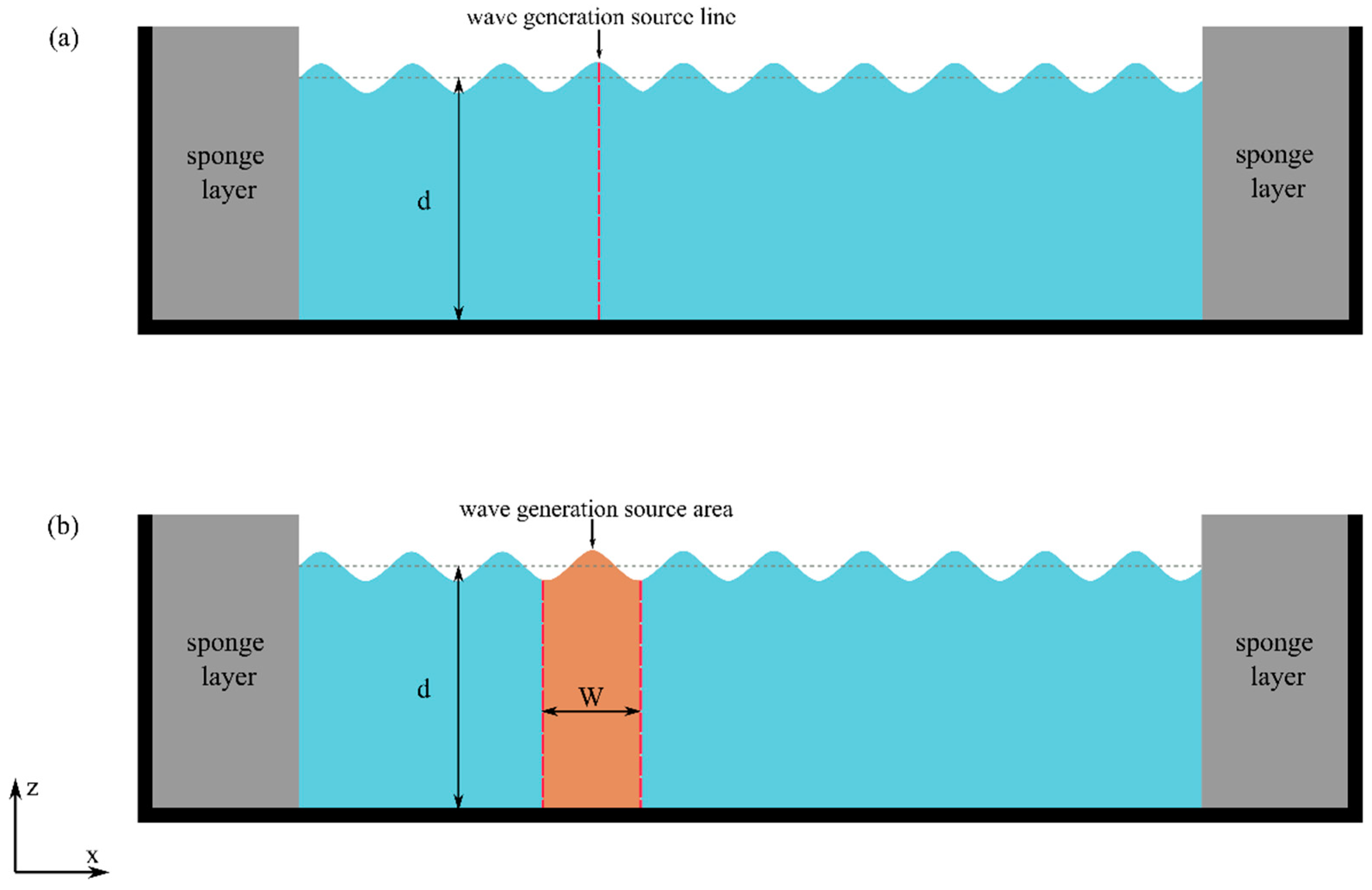
Firstly, the applicability and accuracy of the internal wave generation techniques to generate linear regular waves in transitional and deep water conditions are examined. The numerical basin is similar to the one in Figure 2 with sponge layers at the left and right boundaries with a width of 3$\mathrm{L}$ (where $\mathrm{L}$ is the wave length) and a flat bottom. The internal wave generator is positioned at a distance of 3$\mathrm{L}$ from the sponge layer. 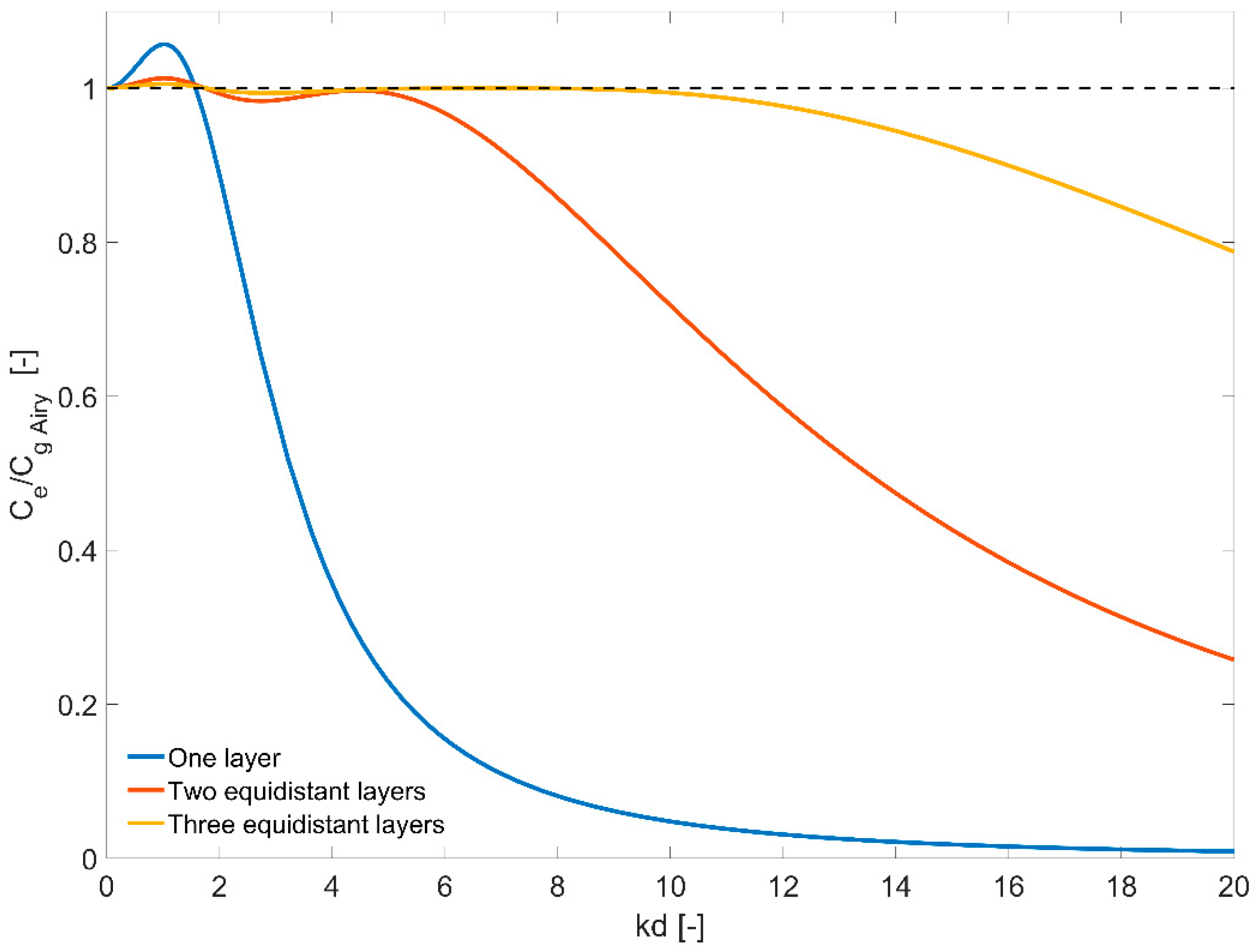Two different wave conditions are examined: one in transitional water ($\mathrm{kd}$ = π/6) and one in deep water ($\mathrm{kd}$ = π, highly dispersive wave). For dimensionless depth $\mathrm{kd}$ = π/6 one vertical layer is applied while for dimensionless depth $\mathrm{kd}$ = π two equidistant vertical layers are applied in order to keep the relative error below 3% (Figure 1, Table 1). For both cases, the grid cell size is chosen so that $\mathsf{\Delta }\mathrm{x}=\mathrm{L}/50$, while the time step is equal to $\mathsf{\Delta }\mathrm{t}\approx \mathrm{T}/350$, where $\mathrm{T}$ is the wave period.

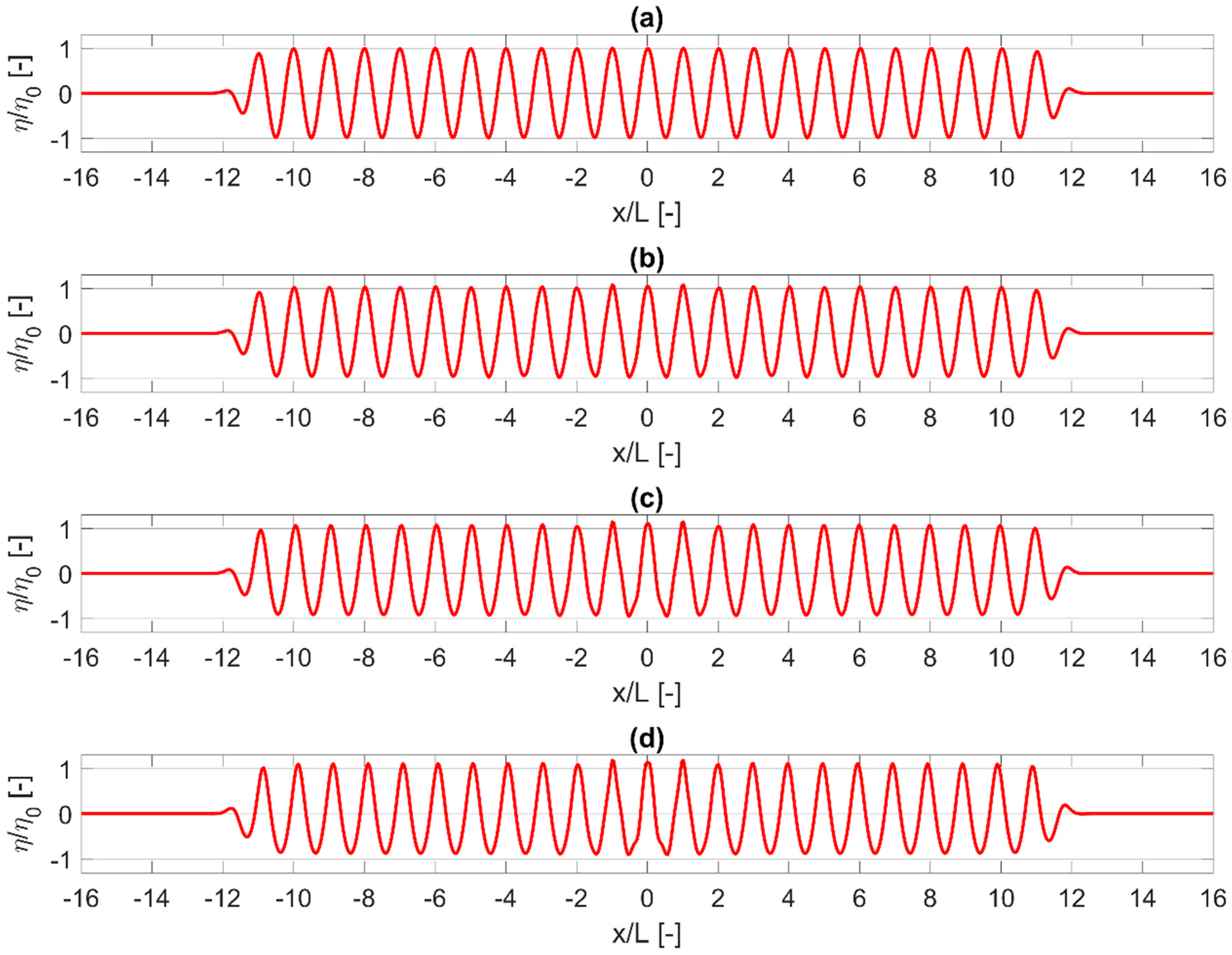
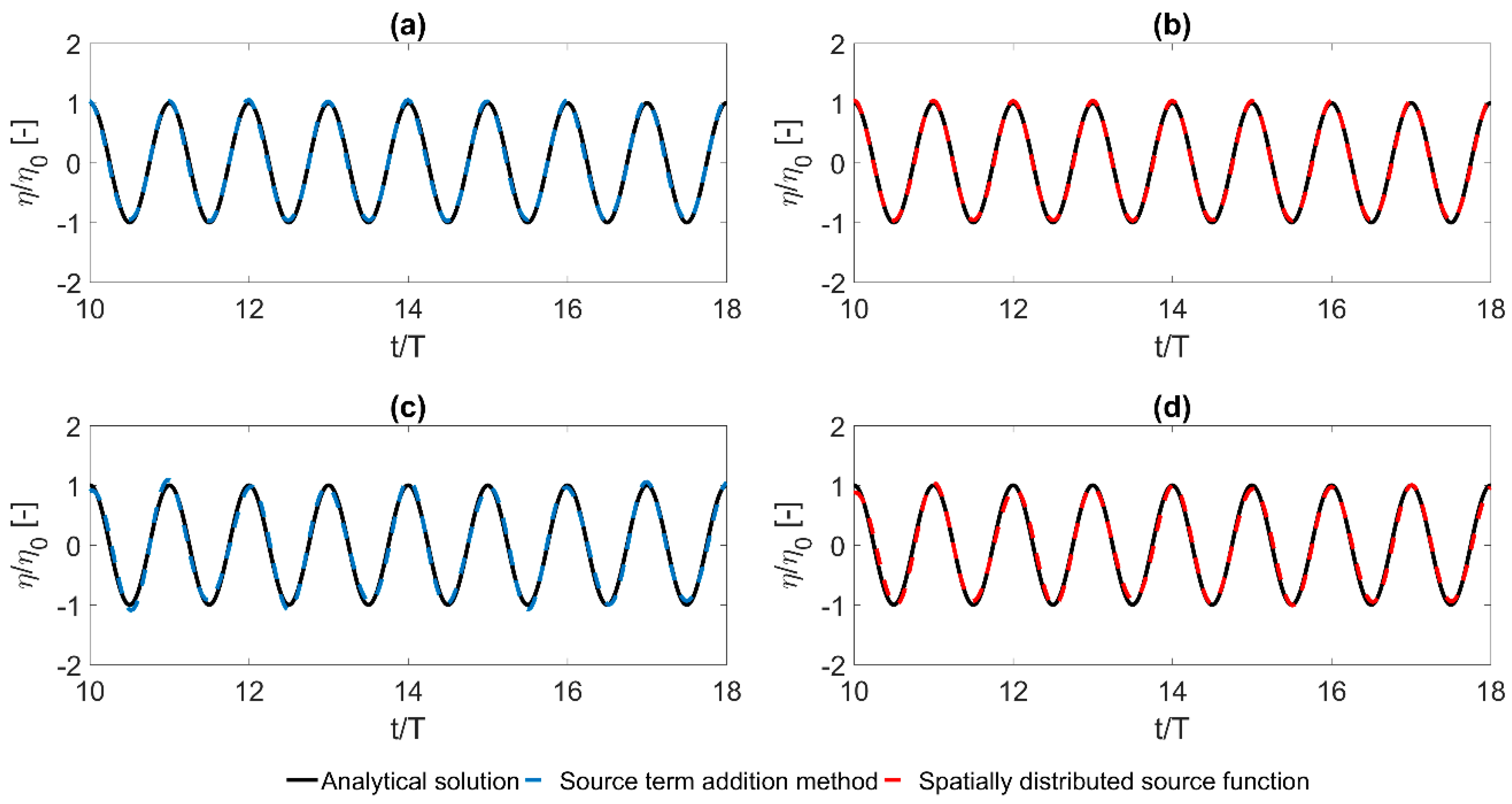
In Figure 3, the normalised water surface elevation $\mathsf{\eta }/{\mathsf{\eta }}_0$ calculated using the source term addition method (blue dashed lines) and the spatially distributed source function (red dashed lines) is presented. The computed results at a distance of 1$\mathrm{L}$ from the internal generator and at a time period of $\mathrm{t}$ = 10$\mathrm{T}$ to $\mathrm{t}$ = 18$\mathrm{T}$ are compared to the results of the analytical solution (solid black lines) for the same conditions. The agreement is very good while the behavior of the two internal wave generation techniques is similar, with a small deviation for the case of the highly dispersive wave (Figure 3c,d). For the latter case, the spatially distributed source function provides a slightly better fit with the analytical solution.

Figure 3. Comparison between computed (dashed lines) and target (solid lines) normalised water surface elevation $\mathsf{\eta }/{\mathsf{\eta }}_0$ for the case of linear waves with dimensionless depth (a,b) $\mathrm{kd}$ = π/6 (one layer) and (c,d) $\mathrm{kd}$ = π (two equidistant layers).

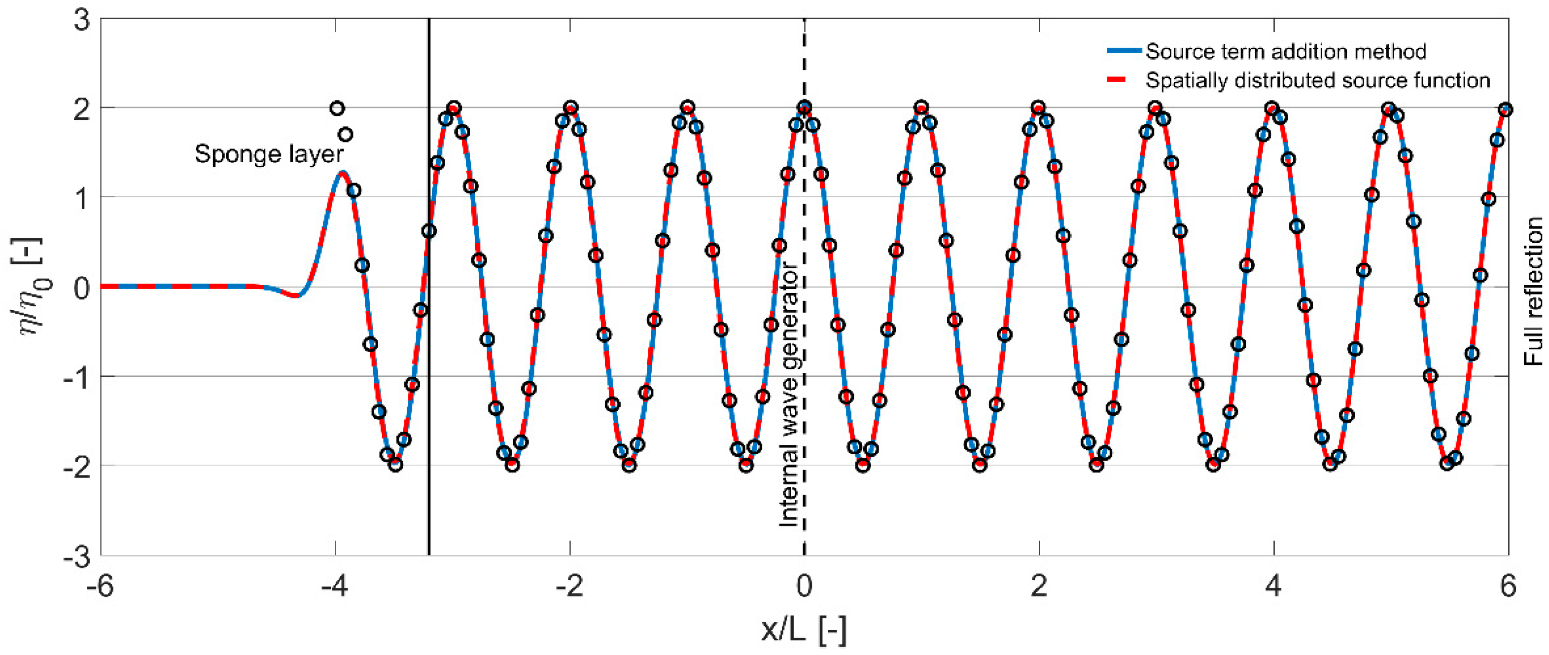
In order to check the capability of the model for handling reflected dispersive waves a computational domain with a sponge layer at the left boundary and a fully reflective wall at the right boundary is used. The internal wave generator is positioned at the middle of the computational domain which has a total length of 12L. The wave height is H = 0.02 m, the wave period is $\mathrm{T}$ = 3 s and the water depth is $\mathrm{d}$ = 10 m. These wave conditions give a dimensionless depth of $\mathrm{kd}$ = 4.5 and thus two equidistant vertical layers are applied. The model is applied with a grid cell size of $\mathsf{\Delta }\mathrm{x}$ = 0.3 m and a time step of $\mathsf{\Delta }\mathrm{t}$ = 0.0125 s.

Figure 4 shows a snapshot of normalised water surface elevation $\mathsf{\eta }/{\mathsf{\eta }}_0$ at $\mathrm{t}$ = 50$\mathrm{T}$ generated using the source term addition method (blue solid line) and the spatially distributed source function (red dashed line). The two computed profiles are identical, while their agreement with the analytical solution (black markers) is excellent.

Figure 4. Snapshot of normalised water surface elevation $\mathsf{\eta }/{\mathsf{\eta }}_0$ at $\mathrm{t}$ = 50$\mathrm{T}$ using two internal wave generation techniques and the analytical solution (black markers) for the case of deep water linear waves ($\mathrm{H}$ = 0.02 m, $\mathrm{T}$ = 3.0 s, $\mathrm{d}$ = 10 m, two equidistant layers) with a sponge layer at the left boundary and a fully reflective wall at the right boundary.

The waves that are generated at the internal wave generator propagate towards both ends of the domain. The waves are fully reflected at the right boundary and then are fully absorbed at the sponge layer. This, together with the fact that the target wave is a linear wave and that the length of the numerical domain is an integer multiple of the wave length, results in a profile that is a standing wave with perfect nodal points. In addition, the results show that the reflected waves pass through the generation area without distortion and that the sponge layer is capable of absorbing the highly dispersive wave. It has to be mentioned that the weakly reflective wave generation (Section 2.2) cannot be applied in this case since the assumption that the reflected waves are shallow water waves propagating with a phase velocity of $\mathrm{C}=\sqrt{\mathrm{gd}}$ is violated.

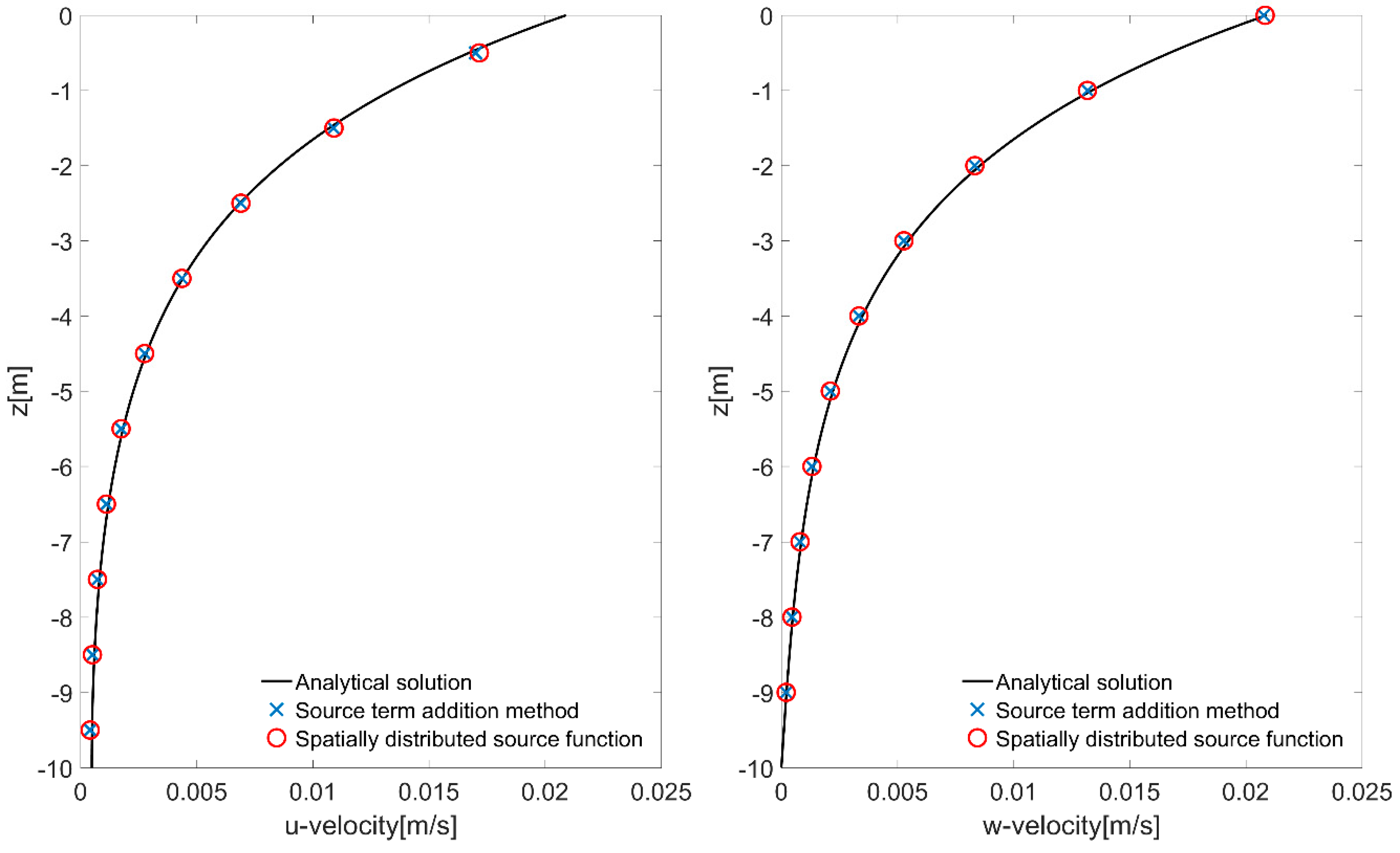
In the proposed internal wave generation techniques, the horizontal velocity component is not prescribed over the vertical direction in contrast to the weakly reflective wave generation (Section 2.2). However, as it can be observed from Figure 5 the horizontal and vertical velocity profiles are correctly calculated for both internal wave generation techniques at a distance of 1$\mathrm{L}$ from the generation point. The wave conditions are the same as in the previous test, while ten equidistant vertical layers have been applied in order to achieve a good agreement with the analytical hyperbolic profile.

Figure 5. Comparison between computed (markers) and target (solid lines) maximum horizontal and vertical velocity profiles using two internal wave generation techniques for the case of deep water linear waves ($\mathrm{H}$ = 0.02 m, $\mathrm{T}$ = 3.0 s, $\mathrm{d}$ = 10 m, ten equidistant layers).

Here, it has to be mentioned that in case of deep water waves, when coarse vertical resolution is applied, the weakly reflective wave generation technique needs calibration to generate the target wave height, since the hyperbolic profile of the horizontal velocity component cannot be accurately described by a small number of vertical layers. On the other hand, the internal wave generation techniques that are presented in this paper do not need calibration, since the source is directly linked with the surface elevation instead of the velocity component.

In all the previous tests in this section, linear waves have been examined. In order to study the behaviour of the internal wave generation techniques under non-linear waves, waves with different wave heights are tested. The internal wave generator is positioned at the middle of the computational domain which has a total length of 32$\mathrm{L}$ with sponge layers at the left and right boundaries and a flat bottom. The wave heights are $\mathrm{H}$ = 0.1 m, 1 m, 2 m, 3 m, while the wave period is $\mathrm{T}$ = 6 s and the water depth is $\mathrm{d}$ = 10 m. These wave conditions give a dimensionless depth of $\mathrm{kd}$ = 1.3 and thus two equidistant vertical layers are applied. The model is applied with a grid cell size of $\mathsf{\Delta }\mathrm{x}$ = 2.0 m and a time step of $\mathsf{\Delta }\mathrm{t}$ = 0.025 s.

Figure 6 shows snapshots of normalised water surface elevation $\mathsf{\eta }/{\mathsf{\eta }}_0$ at $\mathrm{t}=50\mathrm{T}$ for the different wave heights. Profiles generated using the spatially distributed source function are only presented here since the source term addition method becomes unstable for high wave heights. From Figure 6, it can be observed that by increasing the ratio $\mathrm{H}/\mathrm{d}$, the waves are transforming from linear (Figure 6a) to non-linear where the wave crests are becoming sharper and the wave troughs flatter.

Figure 6. Snapshot of normalised water surface elevation $\mathsf{\eta }/{\mathsf{\eta }}_0$ at $\mathrm{t}=50\mathrm{T}$ using the spatially distributed source function wave generation technique for (a) $\mathrm{H}/\mathrm{d}$ = 0.01 (linear), (b) $\mathrm{H}/\mathrm{d}$ = 0.1, (c) $\mathrm{H}/\mathrm{d}$ = 0.2 and (d) $\mathrm{H}/\mathrm{d}$ = 0.3.

4.2. Irregular Waves

We consider two test cases of uni-directional irregular waves fitting a JONSWAP (Joint North Sea Wave Observation Project) spectrum, with a significant wave height, ${\mathrm{H}}_{\mathrm{s}}$ = 0.5 m, a water depth, $\mathrm{d}$ = 10 m, a peak enhancement factor, $\mathsf{\gamma }$ = 3.3 and two different peak wave periods, ${\mathrm{T}}_{\mathrm{p}}$ = 12 s and ${\mathrm{T}}_{\mathrm{p}}$ = 8 s. The frequency range is confined between 0.5${\mathrm{f}}_{\mathrm{p}}$ and 3${\mathrm{f}}_{\mathrm{p}}$. The internal wave generator is positioned at the middle of the computational domain and sponge layers are placed at the left and right boundaries. For both test cases, the model is applied with a grid cell size of $\mathsf{\Delta }\mathrm{x}$ = 1.0 m and a time step of $\mathsf{\Delta }\mathrm{t}$ = 0.025 s. However, for the case of ${\mathrm{T}}_{\mathrm{p}}$ = 8 s two equidistant vertical layers have been applied to correctly describe the high-frequency part of the spectrum in contrast to the case of ${\mathrm{T}}_{\mathrm{p}}$ = 12 s where one layer is enough.

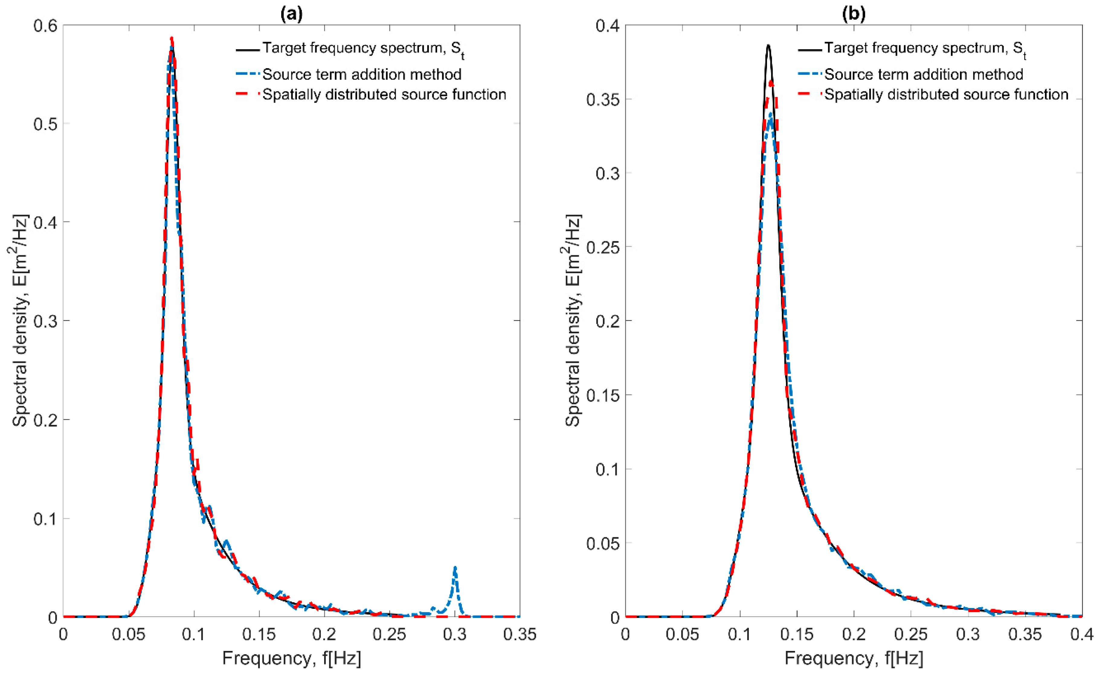
In Figure 7, a comparison is made between the target frequency spectrum (${\mathrm{S}}_{\mathrm{t}}$) and the simulated frequency spectra generated using the two internal wave generation techniques for the cases of ${\mathrm{T}}_{\mathrm{p}}$ = 12 s (Figure 7a) and ${\mathrm{T}}_{\mathrm{p}}$ = 8 s (Figure 7b). The surface elevations $\mathsf{\eta }$ at the electronic wave gauges, which are positioned at a distance of 3${\mathrm{L}}_{\mathrm{p}}$ (where ${\mathrm{L}}_{\mathrm{p}}$ is the wave length corresponding to the peak period) from the internal wave generator, are recorded from $\mathrm{t}=$25${\mathrm{T}}_{\mathrm{p}}$ to $\mathrm{t}=$300${\mathrm{T}}_{\mathrm{p}}$ with a sampling interval of 0.2 s. The recorded data are processed in segments of 2048 points per segment. A taper window and an overlap of 20% are used for smoother and statistically more significant spectral estimates. The resulting frequency spectra agree very well with ${\mathrm{S}}_{\mathrm{t}}$ apart from the one that corresponds to the source term addition method for the case of ${\mathrm{T}}_{\mathrm{p}}$ = 12 s, where high-frequency noise can be observed. In addition, it is found that the magnitude of this noise strongly depends on the grid resolution since a coarser resolution leads to less noise. Moreover, the small difference around the peak of the frequency spectrum in Figure 7b could be caused by numerical dissipation since the electronic wave gauges are positioned at a distance of 3${\mathrm{L}}_{\mathrm{p}}$ from the internal wave generator.

Figure 7. Comparison between the frequency spectra resulting from using two internal wave generation techniques and the target frequency spectrum ${\mathrm{S}}_{\mathrm{t}}$ for irregular waves with ${\mathrm{H}}_{\mathrm{s}}$ = 0.5 m, $\mathrm{d}$ = 10 m (a) ${\mathrm{T}}_{\mathrm{p}}$ = 12 s (one layer) and (b) ${\mathrm{T}}_{\mathrm{p}}$ = 8 s (two equidistant layers).

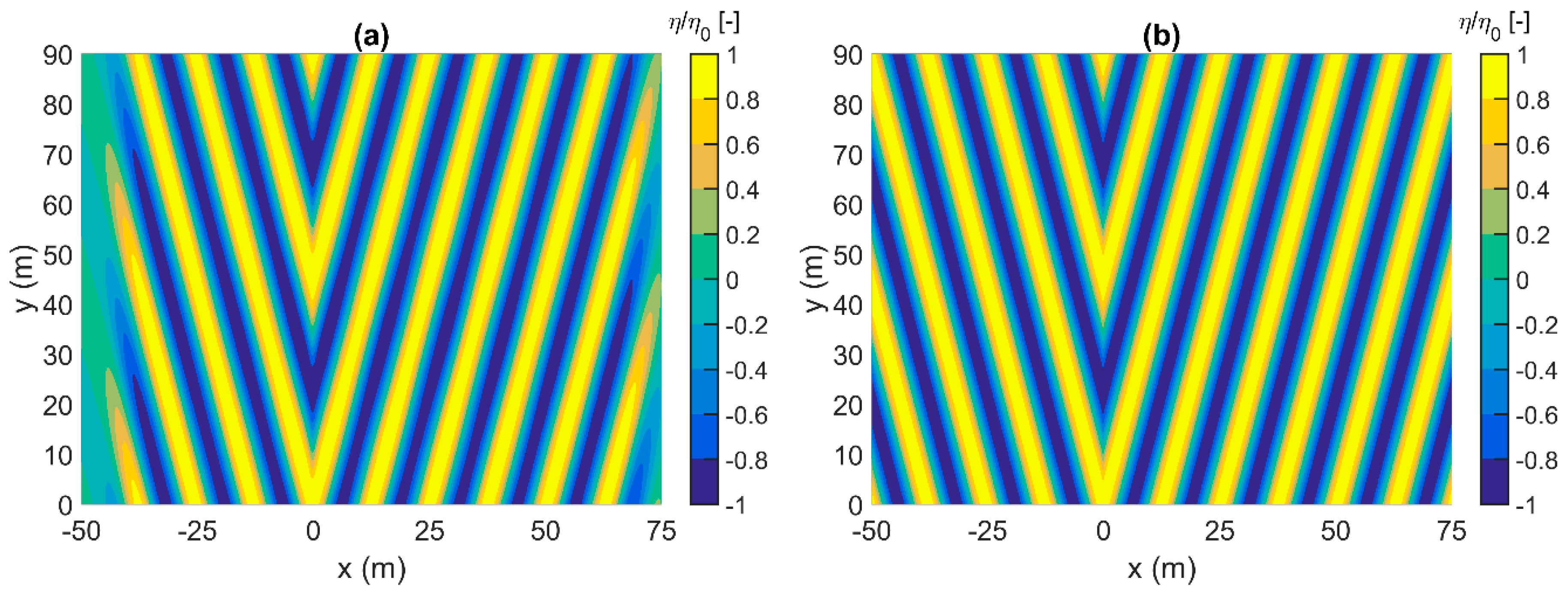
4.3. Oblique Waves in a Basin with Constant Depth

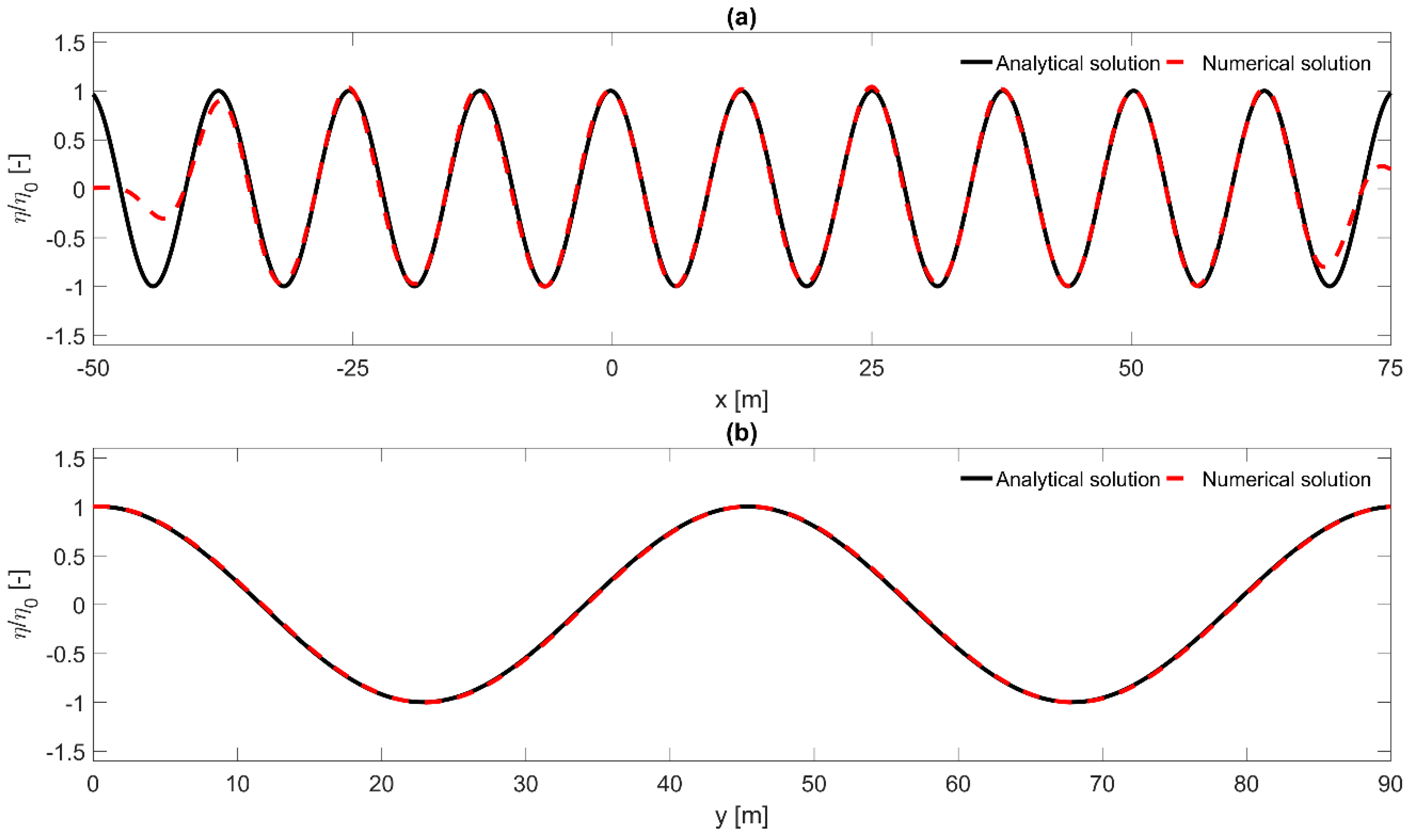
In this section, oblique waves are generated in a basin with constant depth by using the spatially distributed source function wave generation technique. The numerical basin is 190 m long, 90 m wide and 1 m deep. Sponge layers are placed at the left and right boundaries with a width of 50 m while periodic boundaries are applied at the top and bottom of the domain. The internal wave generator is parallel to the y-axis and is positioned at a distance of 100 m (x = 0) from the left boundary. The wave height is $\mathrm{H}$ = 0.01 m, the wave period is $\mathrm{T}$ = 4 s and the wave propagation angle is $\mathsf{\theta }=$15°. The grid cell size is chosen so that $\mathsf{\Delta }\mathrm{x}=\mathsf{\Delta }\mathrm{y}=$0.15 m. In order to obtain a steady state wave field, waves are generated for a duration of 180 s with a time step $\mathsf{\Delta }\mathrm{t}=$0.0125 s.

Figure 8 and Figure 9 present comparisons between the computed normalised water surface elevation $\mathsf{\eta }/{\mathsf{\eta }}_0$ at $\mathrm{t}=40\mathrm{T}$ and the corresponding analytical solution. It can be observed that the computed solution coincides with the analytical solution except for the region of the sponge layers. The excellent agreement indicates that the spatially distributed source function implemented in SWASH is able to accurately generate directional waves.

Figure 8. Comparison between (a) computed and (b) target normalised water surface elevation $\mathsf{\eta }/{\mathsf{\eta }}_0$ at $\mathrm{t}=40\mathrm{T}$ for the case of oblique linear waves ($\mathrm{H}$ = 0.01 m, $\mathrm{T}$ = 4.0 s, $\mathrm{d}$ = 1.0 m and $\mathsf{\theta }$ = 15°) with a sponge layer at the left and right boundaries and periodic boundaries at y–direction.

Figure 9. Comparison between computed (dashed line) and target (solid line) normalised water surface elevation $\mathsf{\eta }/{\mathsf{\eta }}_0$ at $\mathrm{t}=40\mathrm{T}$ for the case of oblique linear waves ($\mathrm{H}$ = 0.01 m, $\mathrm{T}$ = 4.0 s, $\mathrm{d}$ = 1.0 m and $\mathsf{\theta }$ = 15°): (a) cross section at y = 45 m, (b) cross section at x = 0 m.

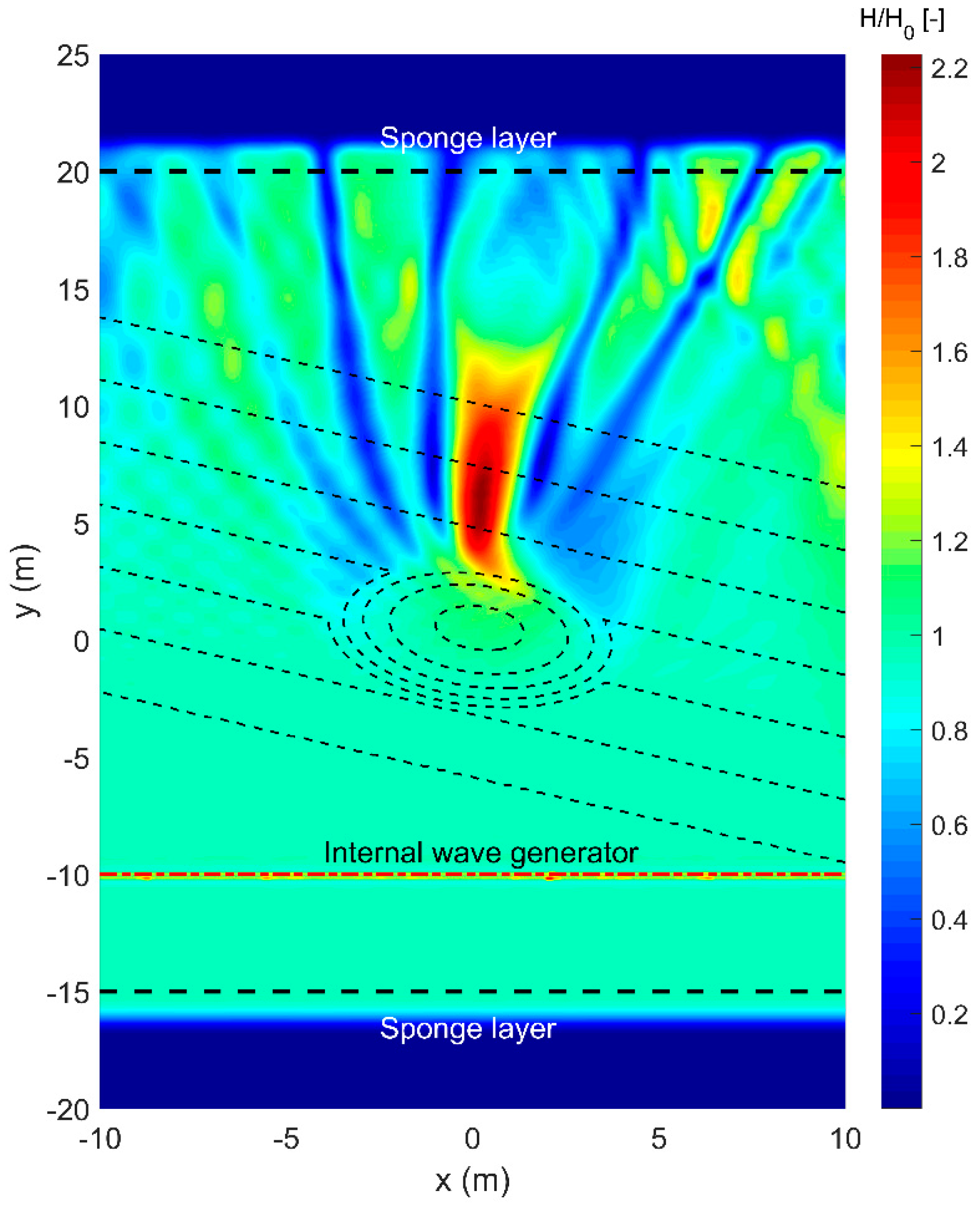
4.4. Wave Propagation over a Shoal in a Three-Dimensional Numerical Basin

Finally, a three-dimensional version of the developed model with the spatially distributed source function wave generation technique is applied to study regular waves propagating over a shoal. The experiment conducted by Reference [33] has served as a standard test case for validating phase resolving wave models.

The bathymetry of the experimental setup consist of an elliptic shoal resting on a plane sloping seabed and the entire slope is turned at an angle of 20° with respect to the x-axis. Detailed information on the geometry can be found in Reference [33]. The numerical basin is 45 m long (−20 < y < 25) and 20 m wide (−10 < x < 10). The internal wave generator is parallel to the x-axis and is positioned at a distance of 10 m (y = −10 m) from the bottom boundary. The remaining numerical domain includes two sidewalls at x = −10 m and x = 10 m and two sponge layers at y = −15 m and y = 20 m with a width of 5 m.

The wave height is $\mathrm{H}$ = 0.0464 m, the wave period is $\mathrm{T}$ = 1 s and the water depth at the position of the internal wave generator is $\mathrm{d}$ = 0.45 m. These wave conditions give a dimensionless depth of $\mathrm{kd}$ = 1.9 and thus two equidistant vertical layers are applied. The model runs for 50 s without any stability issues since the reflected waves that are reaching the offshore boundary are absorbed by the sponge layer, which is positioned behind the internal wave generator. The model is applied with a grid cell size of $\mathsf{\Delta }\mathrm{x}$ = $\mathsf{\Delta }\mathrm{y}$ = 0.05 m, while the time step is automatically adjusted during the simulation depending on the CFL (Courant–Friedrichs–Lewy) condition where a maximum CFL value of 0.5 is used.

Figure 10 shows the plan view of the normalised wave height $\mathrm{H}/{\mathrm{H}}_0$ (where $\mathrm{H}$ is the local wave height and ${\mathrm{H}}_0$ is the wave height at the wave generation boundary) in the whole computational domain where the diffraction and refraction patterns of the waves are visible. The wave heights of the model are obtained by averaging those of the last ten wave periods of the simulation (from t = 40 s to t = 50 s).

Figure 10. Normalised wave height $\mathrm{H}/{\mathrm{H}}_0$ in the whole computational domain for the experiment of Berkhoff [34].

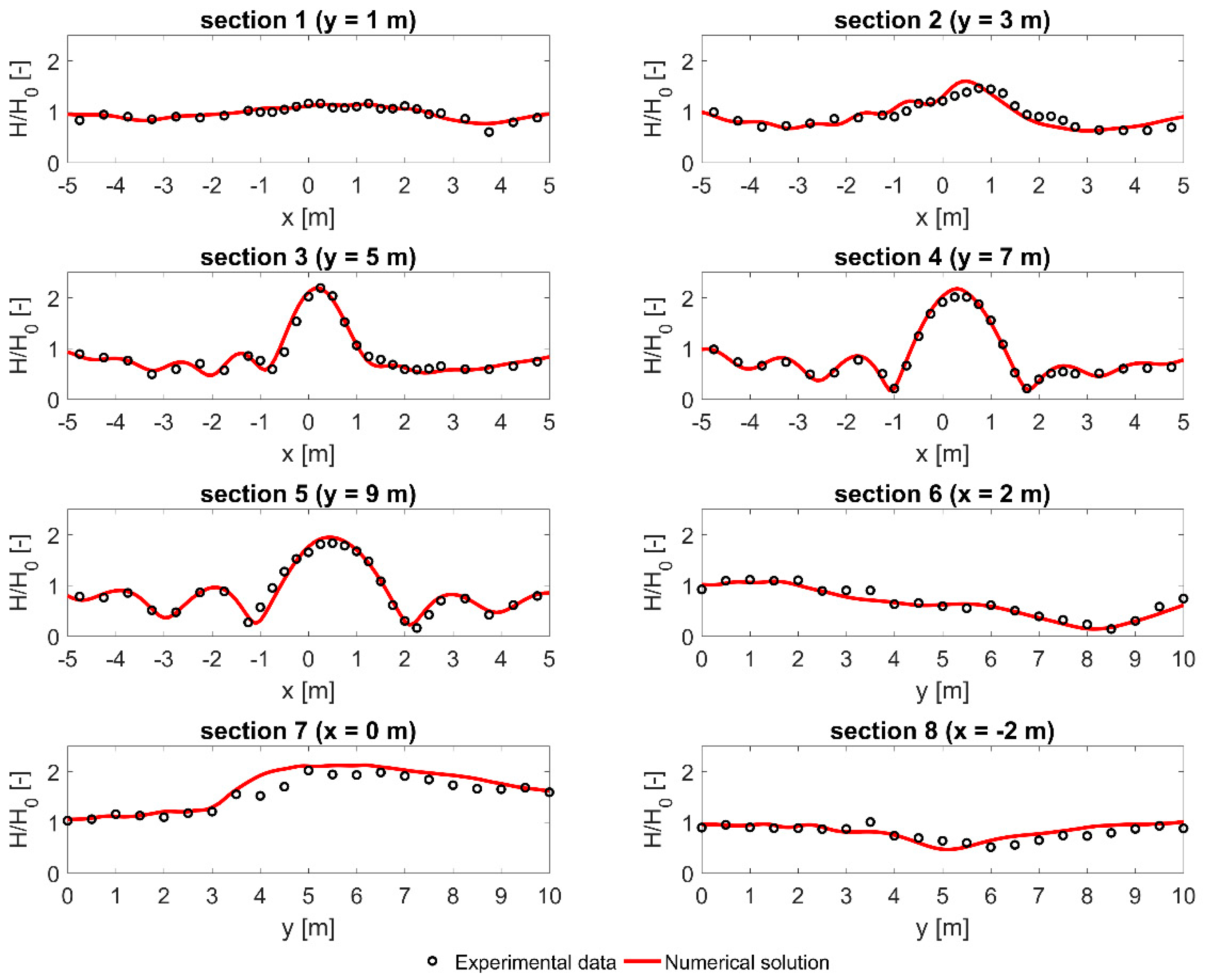
Figure 11 shows the comparison of normalised wave heights $\mathrm{H}/{\mathrm{H}}_0$ between numerical model results (red lines) and experimental data (black circles) along eight measurement transects. Additionally, in order to evaluate the model, the root mean square error (RMSE) and the Skill factor for the normalised wave heights of each section are calculated as:

$$\begin{array}{cc}\mathrm{RMSE}=\sqrt{\frac{{{\displaystyle \sum }}_{\mathrm{i}=1}^{\mathrm{N}}{\left({\mathrm{P}}_{\mathrm{i}}-{\mathrm{O}}_{\mathrm{i}}\right)}^2}{\mathrm{N}}}& \mathrm{Skill}=1-\sqrt{\frac{{{\displaystyle \sum }}_{\mathrm{i}=1}^{\mathrm{N}}{\left({\mathrm{P}}_{\mathrm{i}}-{\mathrm{O}}_{\mathrm{i}}\right)}^2}{{{\displaystyle \sum }}_{\mathrm{i}=1}^{\mathrm{N}}{\mathrm{O}}_{\mathrm{i}}{}^2}}\end{array}$$

(33)

where $\mathrm{O}$ and $\mathrm{P}$ indicate the observed and predicted values, respectively. Very good agreement between the numerical model and the experimental model is observed (Figure 11 and Table 2).

Figure 11. Comparison of normalised wave heights $\mathrm{H}/{\mathrm{H}}_0$ between numerical model results (red solid lines) and experimental data (black circles) along different measurement transects.

Table 2. Root mean square error (RMSE) and Skill factor of the normalised wave heights for each section.

Section	1	2	3	4	5	6	7	8
RMSE	0.056	0.116	0.102	0.074	0.103	0.082	0.157	0.108
Skill	0.944	0.884	0.901	0.929	0.902	0.889	0.901	0.865

5. Conclusions

In the present paper new internal wave generation techniques have been developed in an open source non-hydrostatic wave model, SWASH, for accurate generation of regular and irregular long-crested waves.

Initially, two different internal wave generation techniques have been developed and implemented in SWASH model. The first one is a source term addition method based on the method proposed by Lee et al. [21], while the second one is a spatially distributed source function based on the method proposed by Wei et al. [25]. These techniques need an extension of the numerical domain to accommodate the sponge layer and the source area contrary to the weakly reflective wave generation boundary. Thus, the computational cost increases 15–30%, where the lower values stand for larger computational domains. However, the main advantage of the internal wave generation is that in cases of directional and dispersive waves the reflected waves are absorbed by the sponge layer that is positioned behind the internal wave generator in contrast with the weakly reflective wave generation boundary, which is not valid for these wave conditions due to the limitations as described in Section 2.2. Hence, the internal wave generation has a big advantage when wave energy converter (WEC) farms and man-made structures (e.g., breakwaters, artificial reefs, artificial islands) are examined, since the radiated and reflected waves, respectively, cannot be estimated a priori. In the source term addition method additional surface elevation is added to the calculated surface elevation while in the spatially distributed source function a spatially distributed mass is added in the continuity equation. In both cases, the source term propagates with a velocity which is called the energy velocity which for the system of SWASH equations is mathematically derived in Section 3.1.

Then, these wave generation techniques has been used to generate regular and irregular long-crested waves. The results indicate that the developed model is capable of reproducing the target surface elevations as well as the target frequency spectrum. The overall performance of the spatially distributed source function is better than the source term addition method since the latter becomes unstable for large wave heights and may cause high frequency noise. Finally, the developed model is also used to study wave transformation over an elliptic shoal (Berkhoff shoal experiment) where very good agreement is observed between the numerical model and the experimental results. The aforementioned observations reveal that the spatially distributed source function developed here in SWASH can be successfully used to study coastal areas and wave energy converter (WEC) farms even under highly dispersive and directional waves, while at the same time re-reflections at the position of the wave generator are vanishing.