Abstract
The reservoir operation is a notable source of uncertainty in the natural streamflow and it should be represented in hydrological modelling to quantify the reservoir impact for more effective hydrological forecasting. While many researches focused on the effect of large reservoirs only, this study developed an online reservoir module where the small reservoirs were aggregated into one representative reservoir by employing a statistical approach. The module was then integrated into the coupled Noah Land Surface Model and Hydrologic Model System (Noah LSM-HMS) for a quantitative assessment of the impact of both large and small reservoirs on the streamflow in the upper Gan river basin, China. The Noah LSM-HMS was driven by the China Meteorological Assimilation Driving Datasets for the Soil and Water Assessment Tool (SWAT) model (CMADS) with a very good performance and a Nash-Sutcliffe coefficient of efficiency (NSE) of 0.89, which proved to be more effective than the reanalysis data from the National Centers for Environmental Prediction (NCEP) over China. The simulation results of the integrated model indicate that the proposed reservoir module can acceptably depict the temporal variation in the water storage of both large and small reservoirs. Simulation results indicate that streamflow is increased in dry seasons and decreased in wet seasons, and large and small reservoirs can have equally large effects on the streamflow. With the integration of the reservoir module, the performance of the original model is improved at a significant level of 5%.
1. Introduction
Since decades ago, intensive human activities have brought about a growing challenge to a sustainable watershed management [1,2,3]. In particular, the construction and the management of numerous reservoirs are regarded as a major source of variability and uncertainty in the flow regime [4]. As compared to larger ones, small-scale reservoirs have recently become a preferred choice in the design of hydraulic projects given its cost-effectiveness and its less sociopolitical and environmental consequence. [5,6]. While small reservoirs may be able to provide additional economic benefits, they, together with larger reservoirs, also substantially divide the river basin into small segments, thereby disrupting the natural hydrological processes to a point where conventional hydrologic models without reservoirs are no longer desirable [7].
Hydrological modelling with the consideration of reservoirs have been reported by multiple studies, especially with respect to relatively large-sized reservoirs [8,9]. Hanasaki et al. [10] proposed a generalized reservoir scheme for global river routing models, where reservoirs are regulated using a monthly operation rule for both non-irrigation and irrigation reservoirs. Mateo et al. [4] employed the H08 Water Resources Model and the CaMa-Flood River Routing Model to assess the impact of reservoir operation on the flood propagation. Deng et al. [5] integrated an offline single-reservoir module to Xinanjiang model, a semi-distributed hydrologic model, and made an accurate prediction on the storage and water level change of the studied reservoir. Zhao et al. [11] integrated a reservoir operation module into the Distributed Hydrology-Soil-Vegetation Model (DHSVM) where they employed generalized reservoir operation rules to determine the outflow of reservoir and achieved satisfactory results. All of these studies emphasized the effect of large-scale reservoirs and disregarded the effect of smaller reservoirs.
However, smaller reservoirs should not be excluded in the hydrological modelling in many basins. A survey of Poyang Lake basin in China reveals that there are over 10,000 small reservoirs in the basin accounting for over 1/5 of the combined capacity of all reservoirs. In smaller sub-basins, this value can go up to over a half. Studies involving small reservoirs, however, are relatively scarce but they give some directions. Güntner et al. [12] employed a process-oriented semi-distributed hydrological model to quantify the effect of large and small reservoirs in a semi-arid area in Brazil by aggregating small reservoirs into one large reservoir. However, it does not account for the heterogeneity of water storage or runoff among reservoirs. Cao et al. [13] employed remote sensing techniques to detect the variation in the water surface of small reservoirs before and after the floods to quantify the flood detention effect of the small reservoirs. Deitch et al. [14] developed a Geographic Information System (GIS) based watershed model in which the fine digital elevation model (DEM) and mass-balance equation are employed to assess the cumulative effect of small reservoirs on the downstream flow. It is noted that the function of reservoir to supply water is not considered in their study, which may not be a negligible process in a medium- or long-term hydrological simulation [15]. Besides, most of these studies were based on offline reservoir modules, which can hardly depict the interacting effect of reservoirs on the water cycle.
Finally, meteorological forcing is a crucial impacting factor of the accuracy of hydrological modelling [16]. While rain gauges and meteorological stations traditionally played a significant role in providing forcing data for hydrological models, the recorded data of many stations is hardly accessible for researchers. Additionally, they are often sparsely distributed, especially in mountainous and arid areas [17], and thus are considered less desirable for a fine-scale modelling. The China Meteorological Assimilation Driving Datasets for the SWAT model (CMADS), which was developed by Dr. Xianyong Meng from China Agricultural University, integrates multi-satellite meteorological products with ground observation gauges and has been proven more effective than many of the counterparts since published [18,19,20,21,22,23,24,25]. For instance, Meng et al. [26] applied CMADS to Heihe basin for streamflow simulation and achieved comparatively better performance than other datasets. Similar results were also obtained by Gao et al. [27], who applied CMADS to Xiang River basin. However, the CMADS were mostly applied in the SWAT model so far, whether or not it can desirably drive other land surface models, such as Noah Land Surface Model (Noah LSM) or hydrological models, such as the Hydrologic Model System (HMS), remains a question.
Hence, the first objective of this paper is to develop an online reservoir module in the consideration of particularly small reservoirs and fully integrate this module into a coupled land surface-hydrological model, Noah LSM-HMS. The proposed module aggregated a group of small reservoirs into one representative reservoir using a statistical approach to depict the heterogeneity of storage capacity. Secondly, to have a better understanding of the reservoir impact for more efficient hydrological forecasting for water agencies, the integrated model was applied to the upper Gan River basin, China to depict in detail the effect of both large and small reservoirs on the streamflow. Meanwhile, a comparative study was conducted between the CMADS and the reanalysis data from the National Centers for Environmental Prediction (NCEP) to evaluate the reliability and effectiveness of CMADS, which demonstrates that the CMADS can serve as a reliable dataset to drive hydrological models in China. Simulation results quantitatively indicate that the streamflow is increased in dry seasons and decreased in wet seasons, and large and small reservoirs have equally large effects on the streamflow. With the reservoir module, the performance of the model is also improved.
2. Methods
2.1. The Coupled Land Surface-Hydrological Model System (Noah LSM-HMS)
Noah LSM-HMS is a two-way coupled land surface-hydrological model system developed by Yuan et al. [28] as part of a joint Sino-German research program (hereinafter ‘LSM-HMS’), with its structure being illustrated in Figure 1. Noah LSM is a land surface scheme of the Weather Research and Forecasting Model (WRF) and it is characterized by four soil temperature and moisture layers with canopy moisture and snow cover prediction [29]. It solves the Richards equation to obtain the soil moisture content and the vertical flow, and it employs the water balance and energy balance equations to derive streamflow, evapotranspiration, and recharge, which are then passed on to the hydrological model (HMS). HMS is a spatially distributed hydrological model and it solves the surface and subsurface flow using two-dimensional hydrodynamic equations [30]. HMS also calculates other variables, such as groundwater discharge and vadose-zone soil moisture, and it returns these variables to the LSM. The LSM-HMS is intended to provide a closed description of the water cycle between the land surface and the subsurface and is able to produce reasonable simulations on a range of hydrological variables in a mesoscale basin [29,31,32,33].
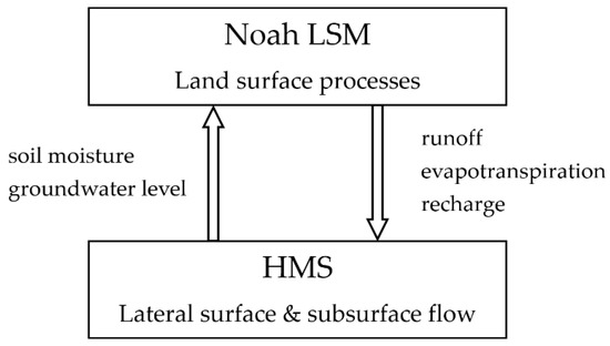
Figure 1.
A schematic diagram of the coupled land surface-hydrological model system.
2.2. Reservoir Modelling
A typical basin, depending on its area, can normally contain up to hundreds or thousands of reservoirs with different capacities. These reservoirs connect each other to form a reservoir system and segment the basin into pieces. To account for the difference of reservoirs in size and importance, a reasonable classification of reservoirs in terms of their capacity is often necessary in the reservoir modelling [12]. In this study, reservoirs with a storage capacity of more than 1 × 10⁷ m3 are categorized as large-sized reservoirs, those with a capacity between 1 ×10⁷ m3 and 1 × 10⁵ m3 are categorized as small-sized. Those with a capacity less than 1 × 10⁵ m3 are regarded as earth dams and pools instead of reservoirs, therefore they are not included in this study.
In view of the scale and the considerable hydrological impact, large reservoirs are directly integrated into grid cells of their actual locations. These reservoirs often function differently with respect to the amount of the incoming flow and the water volume they stored at a certain time. In this study, a simplified operation rule that achieved good performance in Lake Whitney and Lake Aquilla, Texas was employed to estimate the outflow of reservoirs in a daily or monthly scale—see Zhao et al. [11] for more details.
While there are probably not too many of large reservoirs in a typically mesoscale basin, small reservoirs can amount to several hundreds and even thousands, which are dotted everywhere, and most of them do not have larger ones as detailed data. It is thus impractical to quantify the effect of each of them in an analogous way to large reservoirs. A basic idea is to group them to one reservoir, as in the study of Güntner et al. [12] and Malveira et al. [34]. This idea also applies to this study, with the basin of interest divided into a few sub-basins and the small reservoirs in each sub-basin aggregated to a representative reservoir (hereinafter ‘aggregated reservoir’), and the parameters of the aggregated reservoir (e.g., storage capacity) are derived from the summation of all small reservoirs combined. Based on the above idea, the information of heterogeneity in terms of the capacity of each small reservoir is lost. To preliminarily overcome this problem, a capacity cumulative distribution function for small reservoirs in a certain basin is introduced in the form of:
where is the storage capacity of the ith small reservoir sorted in an ascending order and is the portion of small reservoirs that has a capacity less than . It should be noted that the integral of this function on its domain is equal to the mean capacity of the small reservoirs, or the capacity of the aggregated reservoir divided by the number of small reservoirs, N, in the sub-basin. A preliminary curve-fitting study on a few basins of Southeast China suggests that their cumulative distribution function follows a similar pattern, i.e.,
where , i = 1,2,3,4 are the regression coefficients related to basins. Whether or not this distribution pattern suits all basins requires future investigation.
The capacity cumulative distribution function is employed to determine the release of the aggregated reservoirs. To be specific, the mean water storage of all small reservoirs in a sub-basin, (m3), is first calculated from the water storage of the aggregated reservoir divided by the number of small reservoirs. Subsequently, as illustrated in Figure 2, the percentage of small reservoirs with a water storage of smaller than and larger than their storage capacity (i.e., unfilled and filled reservoirs) can be respectively calculated with the mean water storage and the distribution function, and is used to determine the outflow of the aggregated reservoir below.
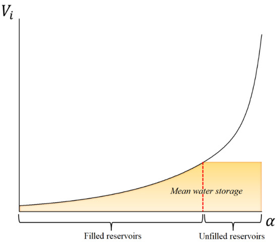
Figure 2.
A schematic illustration of the capacity cumulative distribution function (black curve). The shaded area is the mean water storage of small reservoirs in a sub-basin and can be used to determine the proportion of unfilled and filled reservoirs in this sub-basin.
Given that small reservoirs are mostly used for water supply instead of flood control because of a small capacity, the operation rule is simplified such that, when a reservoir is ‘filled’, all of the water above the capacity will be released immediately and that, when a reservoir is ‘unfilled’, the outflow is determined as the human water demand. The operation rule is then arranged in the following form to determine the reservoir outflow with the consideration of the heterogeneity of capacity:
where (m3/s) and (m3) are the outflow and the water storage of the aggregated reservoir at time t, respectively. (m3/s) is the human water demand. and are the proportion of the combined water storage of unfilled and filled reservoirs, respectively.
After the release of reservoirs is determined, the water balance equation is then employed to calculate (m3), the reservoir water storage at time t:
where (m3) is the water storage of the reservoir for the previous timestep. The initial water storage of reservoir is based on the soil moisture of the local grid. (s) is the timestep. (m2) is the current surface area of the reservoir. and (m3/s) are the inflow and outflow of the reservoir, respectively. (m/s) and E (m/s) are the precipitation and evaporation on the reservoir surface. (m/s) is the two-way flux between the reservoir and the vadose zone or groundwater. It is calculated as a part of the channel-groundwater interaction module in HMS, i.e.,
where (s–1) is the hydraulic conductivity between channel and subsurface. and (m) are respectively the water level of the reservoir and groundwater level.
2.3. Module Integration
By integrating the reservoir module, the model is able to depict the interaction between the reservoir regulation and the subsequent hydrological processes. Firstly, the inflow and release difference due to reservoirs will change the surface water height in the two-dimensional diffusive wave equation and therefore alter the streamflow routing [35]. Secondly, the flux between reservoirs and groundwater will also affect the groundwater depth and the groundwater routing, which is realized by adding an additional source term to the two-dimensional Boussinesq equation. While the surface and subsurface flow routing can directly adjust the streamflow, it can also result in the variation of the hydrological conditions around the reservoirs, e.g., infiltration, river recharge, and groundwater table, which in turn gives feedback to the reservoir operation.
2.4. Performance Indexes
Three indexes are employed for a quantitative evaluation of the downstream streamflow simulation with or without the reservoir module, namely the water balance index (WBI), the Pearson product-moment correlation coefficient (R), and the Nash–Sutcliffe coefficient of efficiency (NSE), for the evaluation of water balance, data correlation, and flood peak simulation, respectively [32,35]:
where and are the simulated and observed streamflow for each timestep, respectively. The overbar symbolizes average.
According to the model evaluation guidelines [36], for a monthly timestep, the model simulation can be considered very good if NSE > 0.75, R > 0.70, and WBI < 0.1.
3. Case Study and Data
3.1. Study Area
The upper Gan River basin, as part of the Yangtze River basin, has an area of around 18,000 km2 (Figure 3). The average annual precipitation is over 1300 mm and it exhibits an uneven distribution within a year. The wet season normally lasts for seven months from March to September, whereas the period from October to February is denoted as dry seasons. The reservoir amount and capacity were stable during the study period of 2008–2015, where there were, in total, about 453 reservoirs in this area, including eight large reservoirs with a combined capacity of 3.78 × 10⁸ m3. The largest reservoir, Tuanjie Reservoir, has a storage capacity of 1.46 × 10⁸ m3. The other 445 small reservoirs have a total storage capacity of 4.25 × 10⁸ m3, with nearly no reservoir newly built or under construction. The small reservoirs account for 98% of the reservoir amount and 53% of the reservoir storage in this basin so that the small reservoirs are supposed to have a considerable cumulative effect on the local hydrologic cycle.
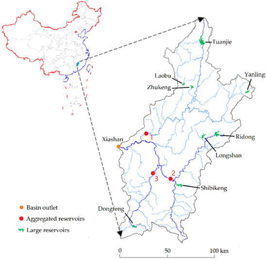
Figure 3.
The upper Gan River basin. Eight large reservoirs are marked in green. Three red round markers with number 1, 2, 3 indicate aggregated reservoirs, which divide the basin into three sub-basins.
3.2. Model Setup
LSM-HMS: The computational timestep for LSM and HMS were determined to be half an hour and one day, respectively, with a spatial resolution of 10 × 10 km. While the study period is 2008–2015, the simulation period starts one year earlier such that the year 2007 is included as part of the model spin-up process.
Reservoir module: The computational domain of LSM-HMS is fully discretized in the unit of grid cell. For large reservoirs, they are directly integrated into the computational grids corresponding to their actual location. However, the integration of aggregated reservoirs is more complicated because they do not really have an actual location or actual amount. Two considerations for the location and number of aggregated reservoirs in this study are presented, as follows:
- The aggregated reservoir can be placed in the proximity of the convergence point between the mainstream and the tributary or between two tributaries so that each tributary is a sub-basin and most of the small reservoirs in the entire basin can be included.
- The number and location of aggregated reservoirs or sub-basins should be in conformity to data availability, so that the sum of the reservoir capacity for each sub-basin can be known.
With the two guidelines above, the detailed configuration of each aggregated reservoir is determined and presented in Table 1. The aggregated reservoirs are generally located downstream three largest tributaries and are around the demarcation of local administrative regions (i.e., counties), such that the reservoir data for each county, e.g., the sum of storage capacity and the number of reservoirs in each sub-basin, are well collected by the local administrations. The study area is therefore divided into three sub-basins with one aggregated reservoir placed at the outlet of each sub-basin, as illustrated in Figure 3.

Table 1.
Configuration of aggregated reservoirs.
3.3. Data Input
The land surface scheme of the model is driven by a set of meteorological forcing. The precipitation, surface air temperature, surface pressure, solar radiation, humidity, and wind speed were obtained from the China Meteorological Assimilation Driving Datasets for the SWAT model (CMADS) [37]. Downward longwave radiation is also needed for the calculation of evapotranspiration and it is obtained from NCEP reanalysis data [38]. The land use and soil data were collected from the Moderate Resolution Imaging Spectroradiometer (MODIS) 1km data and the Harmonized World Soil Database (HWSD), which were both accessed from the Cold and Arid Regions Science Data Center at Lanzhou. The terrain data were obtained from HYDRO1K DEM established by the United States Geological Survey (USGS) [39]. Daily discharge data of Xiashan between 2008–2015 were available for the model calibration and validation.
The yearly water use from reservoirs from 2008–2015 was collected from annual reports that were published by the Department of Water Resources of Jiangxi Province. The irrigation water demand generally accounted for 65% of the total water demand, and it is then evenly downscaled to monthly values throughout the wet seasons. The monthly values are further partitioned to daily values for reservoir input. While the irrigation use occurs during only the irrigation period or wet seasons, other water uses are evenly partitioned from annual to daily values. The water demand of the basin is then allocated to reservoirs in proportion to the storage capacity. Other human activities, including the consumptive use of water and groundwater/river extraction, are not included in this study, since the study focuses on the reservoir effect.
The capacity cumulative distribution function for small reservoirs is fitted using 275 small reservoirs with known capacity in the study area and in the larger Poyang Lake basin, in the form of , and it is assumed to be applicable to the entire basin in this study.
The relationship between water level, surface area and water storage is available for all large reservoirs. For small reservoirs, these correlations are estimated using a linear fitting of the data points from the combination of the large reservoirs.
4. Results and Discussions
In this study, the model was mainly calibrated against the downstream streamflow data series of Xiashan. The calibration and validation period are 2012–2015 and 2008–2011, respectively. The reservoir module was calibrated against the water storage of Tuanjie reservoir from 2012–2015. For conciseness, simulations without the reservoir module, with only large reservoirs and with all reservoirs are hereinafter denoted as LSM-HMS, LH-L, and LH-A, respectively.
4.1. Calibration and Evaluation of the Model
4.1.1. Reservoir Module
To quantify the effect of large reservoirs, the water storage of Tuanjie Reservoir during 2012 and 2015 was employed for the calibration of the operation rule [11]. Subject to the data scarcity, the calibration results were applied to all of the large reservoirs in this study. With respect to Tuanjie Reservoir, the largest reservoir in the basin, the monthly simulation of its storage over the study period and the observation data of its water storage during 2008 and 2015 are illustrated in Figure 4. Most of the simulated water storage follows an increase and decrease alteration within a year, indicating that the reservoir functions well according to the generalized operation rule. The simulation of water storage from 2008 to 2015 generally matches the observation, and the monthly WBI, R, and NSE for the study period are 1.03, 0.84, and 0.65, respectively. A major source of error can be the inaccuracy of inflow computed in LSM-HMS, and the difference between the generalized regulation rule and the reservoir operation in reality is also considered to have greatly contributed to the error. It is especially noted that the water storage of Tuanjie Reservoir is much overestimated, especially in some dry seasons, indicating that the operation rule in reality is very flexible such that the downstream water demand can be satisfied in dryer years. However, this is not presented in the generalized operation rule.
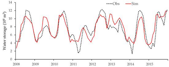
Figure 4.
Monthly simulated and observed water storage of Tuanjie Reservoir during 2008–2015.
4.1.2. LSM-HMS and the Integrated Model
To investigate the impact of the reservoir module on the downstream discharge, the LSM-HMS was calibrated against the monthly observed streamflow discharge in Xiashan for the period of 2012–2015, and then validated in 2008–2011. In all, six parameters were included in the calibration, namely streambed conductivity, Manning’s roughness, saturated hydraulic conductivity, porosity, wilting point, and aquifer thickness. The last four parameters were initially collected from the HWSD database, but it can also be adjusted within a limited range (i.e., ±50%). The calibration results were presented in Table 2.
Table 2.
Calibration results of land surface-hydrological model (LSM-HMS).
In terms of the LSM-HMS, the monthly WBI, R, and NSE are, respectively, 1.03, 0.97, and 0.91 over the calibration period, 1.15, 0.92, and 0.86 over the validation period, and 1.08, 0.95, and 0.89 over the entire study period (see Figure 5). According to the model evaluation guidelines [36], it can be generally regarded as a very good simulation result, indicating that the CMADS-driven LSM-HMS can serve as a reasonable tool to investigate basin-scale hydrological variations and that the CMADS can successfully drive the coupled land surface-hydrological model for an accurate simulation. The error can be attributed to the size of grid cell in this study, as a 10 km grid cell can be too large for a better simulation result in view of the size of the basin. Besides, the spatial heterogeneity of some hydrogeological parameters, such as the wilting point and the Manning coefficient, were not considered, i.e., the entire basin employs a same value because of the data scarcity and model complexity. In addition, the accuracy of CMADS forcing data, after all, is subject to its own spatial resolution and it cannot fully reveal the fine-scale spatial distribution of each meteorological variable. Also, the lack of human activities can also be a source of error in this case.
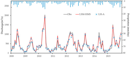
Figure 5.
Monthly observed discharge and simulated discharge of China Meteorological Assimilation Driving Datasets for the SWAT model (CMADS)-driven LSM-HMS and all-reservoir condition (LH-A) in Xiashan during 2008–2015.
By incorporating the effect of large reservoirs, LH-L considers the effect of relatively large reservoirs, thus improving the NSE to 0.90 (1.1%) as compared to LSM-HMS. With the WBI of LH-L decreasing by 2.8% to 1.05, the loss of water is presumably a result of reservoir evaporation and infiltration. With small reservoirs included, it can be seen in Figure 5 that LH-A further improves the simulation. The WBI of LH-A reduces to 1.04 (1.90%) as compared to LH-L for similar reasons. The R and NSE also improve to 0.96 (1.0%) and 0.91 (1.1%) as compared to LH-L, respectively. It is noted that the improvement of LH-A is basically in a same order of magnitude as that of LH-L by comparing the change in WBI, R, and NSE, indicating a large group of small reservoirs can have an effect as considerable as large reservoirs on the streamflow discharge simulation. This effect can be enlarged, especially in this case study where the large reservoirs are all located very upstream with a relatively small capacity than in other typical basins, whereas the small reservoirs are mostly dotted downstream with a larger combined capacity.
A paired Student’s t-Test was also performed to evaluate the magnitude of improvement. The result demonstrates that, for all three sets of comparison, the simulation of downstream streamflow sees a significant improvement at a significant level of 5%, indicating that the proposed reservoir module can effectively reduce the error of the original simulation. The p-values of the t-Test and the performance of each simulation are summarized in Table 3.
Table 3.
Comparison of monthly streamflow simulations.
4.2. Evaluation of CMADS against NCEP Database
Although the model performs well with the CMADS database, it is necessary to compare the accuracy and the efficiency of CMADS with other meteorological databases in driving LSM-HMS. As the existing literature has reported the superiority of CMADS over multiple meteorological data sources, such as the Precipitation Estimation from Remotely Sensed Information using Artificial Neural Networks–Climate Data Record (PERSIANN-CDR) in driving SWAT [25,27], the meteorological reanalysis dataset from NCEP was employed in this section to further evaluate the efficiency of CMADS in LSM-HMS. The NCEP reanalysis data covers the globe in T62 grids and it is widely used in macroscale and mesoscale hydrological modelling. Therefore, the precipitation, air temperature, air pressure, relative humidity, longwave radiation, downward solar radiation, and wind speed were processed and employed in this study to drive LSM-HMS for a comparative study. In general, the NCEP precipitation is 12% larger than the CMADS precipitation for the period of 2008–2015. This is in accordance with the finding of Yang [31] that NCEP tends to overestimate the precipitation in China. The NCEP-driven simulated discharge of Xiashan for 2008–2015 was therefore overestimated by 17% (see Figure 6b), and the WBI, R, and NSE over the study period are 1.17, 0.81, and 0.56, respectively. As also indicated in Figure 6a, the simulation result of NCEP-driven LSM-HMS is much less accurate than that of CMADS-driven LSM-HMS. It suggests that LSM-HMS is sensitive to the input forcing and, when compared to NCEP data, CMADS can serve as a much more reliable source of meteorological forcing for the hydrological modelling in China.
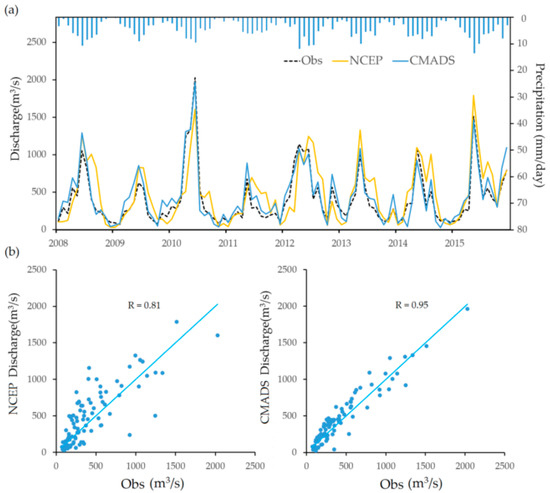
Figure 6.
(a) Monthly observed discharge and simulated discharge of National Centers for Environmental Prediction (NCEP)-driven and China Meteorological Assimilation Driving Datasets for the SWAT model (CMADS)-driven LSM-HMS in Xiashan during 2008–2015, with the NCEP precipitation shown at the top, (b) the scatter plot of observed discharge against NCEP-driven simulation (left) and CMADS-driven simulation (right).
4.3. Effects of Reservoirs on Streamflow
In the previous section, it was found that the introduction of reservoirs can improve the performance of Noah LSM-HMS at a significant level of 5%. The temporal distribution of the difference between all-reservoir condition (LH-A) and no-reservoir condition (LSM-HMS) was presented in Figure 7. It can be seen that the improvement in LH-A as compared to LSM-HMS can be mostly attributed to the increase of streamflow in dry seasons and the decrease of streamflow in wet seasons, since reservoirs can be regulated to mitigate the flood in wet seasons and to supply water in dry seasons. To be specific, the streamflow sees a 5.1 m3/s (2.0%) increase in dry seasons and a 45.4 m3/s decrease (7.8%) in wet seasons. In light of the different modelling methods between large and small reservoirs, their effects are separately discussed, as follows.
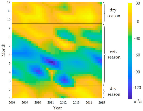
Figure 7.
Temporal distribution of reservoir effect on the downstream discharge at Xiashan for 2008–2015. Yellow indicates the streamflow is increased with the consideration of reservoirs whereas blue indicates otherwise (see the color bar).
Large reservoirs: Large reservoirs are generally intended to mitigate floods in wet seasons and supply more water in dry seasons. To quantitatively explain the simulated effects of the large reservoirs on extreme climate conditions, the averaged maximum monthly inflow (high flow) and minimum monthly inflow (low flow), and the release of each reservoir were selected and presented in Table 4. It is noted that, for all large reservoirs, the maximum monthly inflow is reduced, with the largest reduction of 53.5% for the Shibikeng Reservoir. On the other hand, the monthly low flow is maintained or increased for all of the reservoirs except Ridong Reservoir. These results indicate that, with the generalized operation rule, the large reservoirs effectively mitigate floods and, in most cases, supply more water in dry seasons.
Table 4.
Effects of reservoirs on the monthly maximum and minimum flow.
Small reservoirs: While most small reservoirs are not primarily intended for flood mitigation because of the limited capacity, a large group of small reservoirs can indirectly reduce the local floods because there is always a portion of small reservoirs that are not filled enough to release all of the incoming flood. For example, the simulated inflow and outflow of small reservoirs represented by aggregated reservoir 3 for the first half of 2010 are illustrated in Figure 8b, where the flood peaks are mitigated by different minor values. As the wet season arrives, the proportion of unfilled and filled small reservoirs in the sub-basin is constantly changing in terms of the magnitude of the incoming flow (see Figure 8a). An increasing number of small reservoirs become dry towards the end of dry season because of the human water demand. When the flood season comes, these reservoirs start to fill up as the flood peaks are somewhat reduced. It is also noted that, due to the limited capacity, most of the small reservoirs are filled during a significant flood where almost all of the flood is released immediately.
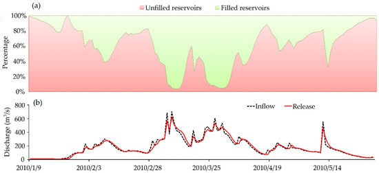
Figure 8.
For small reservoirs represented by aggregated reservoir 3, (a) the daily simulated percentage of unfilled and filled small reservoirs, and (b) the corresponding simulated inflow and release of the aggregated reservoir 3 during January and May 2010.
The averaged maximum and minimum monthly inflow and outflow of each aggregated reservoir are presented in Table 4. It can be seen the relative flood mitigation effect of aggregated reservoirs is minor (0.7%–2.5%) as compared to large reservoirs, but the absolute value of mitigation is not necessarily smaller than large reservoirs. In a monthly level, the small reservoirs can increase the local runoff by 0%–21% in dry seasons, indicating that small reservoirs can serve as an effective source of human water use in dry seasons.
For a more direct view of the effect of reservoirs, three flood events are selected for comparison between LSM-HMS and LH-A. It can be seen from Figure 9 that the flood peaks are mitigated by different values. For instance, with respect to the floods on January 2008, May 2009, and April 2013, the peak discharges simulated by LH-A are, respectively, 95 m3/s, 120 m3/s, and 108 m3/s lower than those simulated by LSM-HMS alone, making the simulated values closer to the observed ones. Similarly, a flood detention effect can be observed in some flood events, i.e., the flood tends to rise and fall less drastically in the simulation of LH-A (see also Figure 9). This effect is more conspicuous, especially for the first flood after a long relatively dry period, presumably because the reservoir group needs to fill themselves first before releasing the flood.
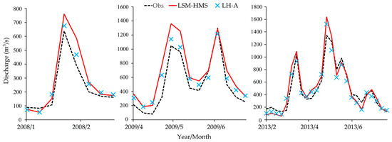
Figure 9.
Comparison of weekly mean observed downstream streamflow in Xiashan and simulated streamflow of LH-A and LSM-HMS for three selected periods.
5. Conclusions
Reservoir operation can result in notable uncertainty in terms of hydrological modelling and it is an important aspect that should be handled to gain better knowledge of the reservoir impact and to support a more effective hydrological forecasting for water agencies. While carrying out detailed investigations on the regulation scheme of each reservoir is time-consuming and impractical, especially for small reservoirs, this paper aggregated small reservoirs into one representative reservoir with the use of the capacity cumulative distribution function, which was then integrated into a coupled land surface-hydrological model, Noah LSM-HMS. Large important reservoirs were also represented in the model using a set of generalized operation rules. With the application of the integrated model to a case study in the upper Gan river basin, the following conclusions are made:
- CMADS can serve as a high-quality meteorological database for the coupled land surface-hydrological model. CMADS-driven LSM-HMS generally have a much better performance than NCEP-driven LSM-HMS.
- The reservoir module can depict the annual and interannual variation in the water storage well for both large and small reservoirs. The integrated model yields improved simulation results at a significant level with the incorporation of reservoirs.
- Both large reservoirs and small reservoirs have a similar effect in reducing the floods in wet seasons and increasing the flow in dry seasons. Although small reservoirs are not primarily intended for flood mitigation, a large group of small reservoirs can indirectly reduce the local floods by up to 2.5% in a monthly level.
- The error of LSM-HMS is related to the input data and grid resolution as well as input parameter error. With a finer modelling resolution, the error is expected to be reduced. The simplification of the reservoir representation and the operation rule is also considered to be a source of error.
The idea using a statistical distribution and an aggregated reservoir to represent small reservoirs in this study serves as a compromise between the convenience and model accuracy. It saves time from investigating and integrating each of the small reservoirs, especially in a basin where there are too many small reservoirs to consider one by one. However, this idea of introducing aggregated reservoirs, after all, is based on a lumped hydrologic concept rather than a distributed concept to be used in a distributed hydrological model. While one can employ a more distributed method by, for example, distributing one or more reservoirs into each of the grid, their interconnection in the model needs to be considered with care to be an appropriate representation of the reality, and further work is expected on this aspect.
The idea using a statistical distribution and an aggregated reservoir to represent small reservoirs in this study serves as a compromise between the convenience and model accuracy. It saves time from investigating and integrating each of the small reservoirs, especially in a basin where there are too many small reservoirs to consider one by one. However, this idea of introducing aggregated reservoirs, after all, is based on a lumped hydrologic concept rather than a distributed concept to be used in a distributed hydrological model. While one can employ a more distributed method by, for example, distributing one or more reservoirs into each of the grid, their interconnection in the model needs to be considered with care to be an appropriate representation of the reality, and further work is expected on this aspect.
Author Contributions
Conceptualization: M.Y., X.M., H.W. and C.Y., Investigation: X.L., X.M., C.Y. and Z.W., Methodology: N.D., X.M., H.W. and M.Y., Formal analysis: N.D., X.L. and Z.W., Writing: N.D. All the authors have approved of the submission of this manuscript.
Funding
Financial support for this study was provided by the National Key Research and Development Project (2016YFC0402201), the National Science Foundation for Young Scientists of China (Grant No.51709271), the Young Elite Scientists Sponsorship Program by CAST (2017QNRC001) and the National Natural Science Foundation of China (41761134090; 41323001; 41471016).
Acknowledgments
Special thanks to Jianhui Wei and Qing Zhao for providing instructions and suggestions on this work.
Conflicts of Interest
The authors declare no conflict of interest.
References
- Zhang, L.; Karthikeyan, R.; Bai, Z.; Wang, J. Spatial and temporal variability of temperature, precipitation, and streamflow in upper sang-kan basin, china. Hydrol. Process. 2018, 31, 279–295. [Google Scholar] [CrossRef]
- Yang, L.; Feng, Q.; Yin, Z.; Wen, X.; Si, J.; Li, C.; Deo, R.C. Identifying separate impacts of climate and land use/cover change on hydrological processes in upper stream of Heihe River, Northwest China. Hydrol. Process. 2017, 31, 1100–1112. [Google Scholar] [CrossRef]
- Marhaento, H.; Booij, M.J.; Rientjes, T.H.M.; Hoekstra, A.Y. Attribution of changes in the water balance of a tropical catchment to land use change using the SWAT model. Hydrol. Process. 2017, 31, 2029–2040. [Google Scholar] [CrossRef]
- Mateo, C.M.; Hanasaki, N.; Komori, D.; Tanaka, K.; Kiguchi, M.; Champathong, A.; Sukhapunnaphan, T.; Dai Yamazaki, D.; Oki, T. Assessing the impacts of reservoir operation to floodplain inundation by combining hydrological, reservoir management, and hydrodynamic models. Water. Resour. Res. 2015, 50, 7245–7266. [Google Scholar] [CrossRef]
- Deng, C.; Liu, P.; Liu, Y.; Wu, Z.; Wang, D. Integrated hydrologic and reservoir routing model for real-time water level forecasts. J. Hydrol. Eng. 2014, 20, 05014032. [Google Scholar] [CrossRef]
- Mushtaq, S.; Dawe, D.; Hafeez, M. Economic evaluation of small multi-purpose ponds in the Zhanghe irrigation system, China. Agric. Water. Manag. 2007, 91, 61–70. [Google Scholar] [CrossRef]
- Potter, K.W. Small-scale, spatially distributed water management practices: Implications for research in the hydrologic sciences. Water. Resour. Res. 2006, 42. [Google Scholar] [CrossRef]
- Christensen, N.S.; Lettenmaier, D.P. A multimodel ensemble approach to assessment of climate change impacts on the hydrology and water resources of the Colorado River Basin. Hydrol. Earth Syst. Sci. Discuss. 2006, 3, 3727–3770. [Google Scholar] [CrossRef]
- VanRheenen, N.T.; Wood, A.W.; Palmer, R.N.; Lettenmaier, D.P. Potential implications of PCM climate change scenarios for Sacramento–San Joaquin River Basin hydrology and water resources. Clim. Chang. 2004, 62, 257–281. [Google Scholar] [CrossRef]
- Hanasaki, N.; Kanae, S.; Oki, T. A reservoir operation scheme for global river routing models. J. Hydrol. 2006, 327, 22–41. [Google Scholar] [CrossRef]
- Zhao, G.; Gao, H.; Naz, B.S.; Kao, S.C.; Voisin, N. Integrating a reservoir regulation scheme into a spatially distributed hydrological model. Adv. Water. Resour. 2016, 98, 16–31. [Google Scholar] [CrossRef]
- Güntner, A.; Krol, M.S.; Araújo, J.C.D.; Bronstert, A. Simple water balance modelling of surface reservoir systems in a large data-scarce semiarid region/Modélisation simple du bilan hydrologique de systèmes de réservoirs de surface dans une grande région semi-aride pauvre en données. Hydrol. Sci. J. 2014, 49. [Google Scholar] [CrossRef]
- Cao, M.; Zhou, H.; Zhang, C.; Zhang, A.; Li, H.; Yang, Y. Research and application of flood detention modeling for ponds and small reservoirs based on remote sensing data. Sci. China Tech. Sci. 2011, 54, 2138–2144. [Google Scholar] [CrossRef]
- Deitch, M.J.; Merenlender, A.M.; Feirer, S. Cumulative effects of small reservoirs on streamflow in Northern Coastal California catchments. Water Resour. Manag. 2013, 27, 5101–5118. [Google Scholar] [CrossRef]
- Magilligan, F.J.; Nislow, K.H. Changes in hydrologic regime by dams. Geomorphology 2005, 71, 61–78. [Google Scholar] [CrossRef]
- Salamon, P.; Feyen, L. Assessing parameter, precipitation, and predictive uncertainty in a distributed hydrological model using sequential data assimilation with the particle filter. J. Hydrol. 2009, 376, 428–442. [Google Scholar] [CrossRef]
- Guo, B.; Zhang, J.; Xu, T.; Croke, B.; Jakeman, A.; Song, Y.; Yang, Q.; Lei, X.; Liao, W. Applicability Assessment and Uncertainty Analysis of Multi-Precipitation Datasets for the Simulation of Hydrologic Models. Water 2018, 10, 1611. [Google Scholar] [CrossRef]
- Cao, Y.; Zhang, J.; Yang, M. Application of SWAT Model with CMADS Data to Estimate Hydrological Elements and Parameter Uncertainty Based on SUFI-2 Algorithm in the Lijiang River Basin, China. Water 2018, 10, 742. [Google Scholar] [CrossRef]
- Meng, X.; Wang, H.; Shi, C.; Wu, Y.; Ji, X. Establishment and Evaluation of the China Meteorological Assimilation Driving Datasets for the SWAT Model (CMADS). Water 2018, 10, 1555. [Google Scholar] [CrossRef]
- Meng, X.; Wang, H.; Wu, Y.; Long, A.; Wang, J.; Shi, C.; Ji, X. Investigating spatiotemporal changes of the land-surface processes in Xinjiang using high-resolution CLM3.5 and CLDAS: Soil temperature. Sci. Rep. 2017, 7, 13286. [Google Scholar] [CrossRef]
- Meng, X.; Wang, H. Significance of the China Meteorological Assimilation Driving Datasets for the SWAT Model (CMADS) of East Asia. Water 2017, 9, 765. [Google Scholar] [CrossRef]
- Meng, X.; Dan, L.; Liu, Z. Energy balance-based SWAT model to simulate the mountain snowmelt and runoff—Taking the application in Juntanghu watershed (China) as an example. J. Mt. Sci. 2015, 12, 368–381. [Google Scholar] [CrossRef]
- Meng, X.; Wang, H.; Lei, X.; Cai, S.; Wu, H. Hydrological Modeling in the Manas River Basin Using Soil and Water Assessment Tool Driven by CMADS. Teh. Vjesn. 2017, 24, 525–534. [Google Scholar] [CrossRef]
- Zhao, F.; Wu, Y. Parameter Uncertainty Analysis of the SWAT Model in a Mountain Loess Transitional Watershed on the Chinese Loess Plateau. Water 2018, 10, 690. [Google Scholar] [CrossRef]
- Liu, J.; Shanguan, D.; Liu, S.; Ding, Y. Evaluation and Hydrological Simulation of CMADS and CFSR Reanalysis Datasets in the Qinghai-Tibet Plateau. Water 2018, 10, 513. [Google Scholar] [CrossRef]
- Meng, X.; Wang, H.; Cai, S.; Zhang, X.; Leng, G.; Lei, X.; Shi, C.; Liu, S.; Shang, Y. The China Meteorological Assimilation Driving Datasets for the SWAT Model (CMADS) Application in China: A Case Study in Heihe River Basin. Pearl River 2016, 37, 1–9. [Google Scholar]
- Gao, X.; Zhu, Q.; Yang, Z.; Wang, H. Evaluation and Hydrological Application of CMADS against TRMM 3B42V7, PERSIANN-CDR, NCEP-CFSR, and Gauge-Based Datasets in Xiang River Basin of China. Water 2018, 10, 1225. [Google Scholar] [CrossRef]
- Yuan, F.; Kunstmann, H.; Yang, C.; Yu, Z.; Ren, L.; Fersch, B.; Xie, Z. Development of a coupled land-surface and hydrology model system for mesoscale hydrometeorological simulations. In New Approaches to Hydrological Prediction in Data-Sparse Regions, Proceedings of Symposium HS.2 at the Joint Convention of the International Association of Hydrological Sciences (IAHS) and The International Association of Hydrogeologists (IAH), Hyderabad, India, 6–12 September 2009; IAHS Press: Wallingford, UK, 2009. [Google Scholar]
- Wagner, S.; Fersch, B.; Yuan, F.; Yu, Z.; Kunstmann, H. Fully coupled atmospheric-hydrological modeling at regional and long-term scales: Development, application, and analysis of WRF-HMS. Water Resour. Res. 2016, 52, 3187–3211. [Google Scholar] [CrossRef]
- Yu, Z.; Pollard, D.; Cheng, L. On continental-scale hydrologic simulations with a coupled hydrologic model. J. Hydrol. 2006, 331, 110–124. [Google Scholar] [CrossRef]
- Yang, C. Research on Coupling Land Surface-Hydrology Model and Application. Ph.D. Thesis, Hohai University, Nanjing, China, 2009. [Google Scholar]
- Yang, C.; Lin, Z.; Yu, Z.; Hao, Z.; Liu, S. Analysis and simulation of human activity impact on streamflow in the Huaihe River basin with a large-scale hydrologic model. J. Hydrometeorol. 2010, 11, 810–821. [Google Scholar] [CrossRef]
- Yang, C.; Yu, Z.; Hao, Z.; Zhang, J.; Zhu, J. Impact of climate change on flood and drought events in Huaihe River Basin, China. Hydrol. Res. 2012, 43, 14–22. [Google Scholar] [CrossRef]
- Malveira, V.T.C.; Araújo, J.C.D.; Güntner, A. Hydrological impact of a high-density reservoir network in semiarid northeastern Brazil. J. Hydrol. Eng. 2011, 17, 109–117. [Google Scholar] [CrossRef]
- Lv, M.; Hao, Z.; Lin, Z.; Ma, Z.; Lv, M.; Wang, J. Reservoir operation with feedback in a coupled land surface and hydrologic model: A case study of the Huai River Basin, China. J. Am. Water Resour. Assoc. 2016, 52, 168–183. [Google Scholar] [CrossRef]
- Moriasi, D.N.; Arnold, J.G.; Liew, M.W.V.; Bingner, R.L.; Harmel, R.D.; Veith, T.L. Model evaluation guidelines for systematic quantification of accuracy in watershed simulations. Trans. ASABE 2007, 50, 885–900. [Google Scholar] [CrossRef]
- The China Meteorological Assimilation Driving Datasets for the SWAT model (CMADS). Available online: http://www.cmads.org (accessed on 25 October 2018).
- NOAA Earth System Research Laboratory. Available online: https://www.esrl.noaa.gov (accessed on 26 October 2018).
- USGS EROS Archive-Digital ElevationHYDRO1K. Available online: https://www.usgs.gov/centers/eros/science/usgs-eros-archive-digital-elevation-hydro1k (accessed on 1 October 2018).
© 2019 by the authors. Licensee MDPI, Basel, Switzerland. This article is an open access article distributed under the terms and conditions of the Creative Commons Attribution (CC BY) license (http://creativecommons.org/licenses/by/4.0/).