Spatial and Temporal Trend Analysis of Precipitation and Drought in South Korea

Abstract

High spatial and temporal variation in precipitation in South Korea leads to an increase in the frequency and duration of drought. In this study, the spatial characteristics of temporal trends for precipitation and drought severity time series were analyzed at 55 stations across South Korea for the period 1980–2015. This study also reviewed the usefulness of different trend tests while addressing the issue of serial correlation, which has often received less attention in previous studies. Results showed that most significant trends in precipitation were detected along the south coast of South Korea, especially during winter, late spring and summer, whereas no significant trend was detected in annual precipitation. The Sen’s slope of the trends increased from January to August and decreased from August onward. Principal component analysis applied on Standardized Precipitation Index (SPI) at a 12-month time scale divides the whole of South Korea into four subregions with different temporal behaviors of drought severity. Moreover, drought severity showed a significant increasing trend, mainly on the northeast coast. Drought frequency analysis showed more frequent droughts in late winter, early spring and early autumn, with less frequent droughts in summer.

1. Introduction

Drought is a natural phenomenon, and it occurs with spatiotemporal variation in frequency, severity, and duration. Moreover, drought can be characterized as both a hazard and a disaster [1]. Trends in drought frequency, duration or severity can be expressed through the changes in precipitation [2]. Since precipitation is a highly important climatic variable and has a direct impact on the occurrence of drought [3,4,5] or flood [6,7], joint trend analysis of drought and precipitation has been gaining more importance in recent studies [2,8,9,10]. Identification of trends in precipitation and drought helps to understand the long-term variation of hydrometeorological processes and explore their periodicities [11].

Precipitation in South Korea has high spatial and temporal variability. The complex topographical and climatic characteristics of South Korea lead to greater variation in annual precipitation in the southern part (1000 mm to 1800 mm) than the central part (1100 mm to 1400 mm). This climatic variability is the main problem for water resource management in South Korea, especially during water shortage periods. To cope with this problem, the spatial and temporal variation of precipitation has been analyzed in previous studies in South Korea [12,13,14]; however, the spatial and temporal variability of drought based on Principal Component Analysis (PCA) to compare the temporal behavior of regional drought patterns has never been studied before.

We recognize that the robustness of significance testing for hydroclimatic indicators has been increasingly questioned in recent literature due to difficulties in establishing a valid null hypothesis and the impact of long-term persistence (e.g., [15,16]. This increase in criticism is because hydro-climatic data often violate the assumptions required for statistical testing (such as distribution, correlations and stationarity of the data). This study deals with the correlation assumption of the data. Although several attempts have been made to analyze the precipitation trends in South Korea, with most of them focusing only on the summer or seasonal precipitation trends [12,14,17,18,19] and others focusing on the trends in total precipitation [13,20,21,22,23,24,25], no comprehensive research has been conducted on drought severity trends in South Korea. In most of the previous studies, the precipitation trends were detected using non-parametric techniques, especially the Mann-Kendall test, without paying any attention to the serial structure of the time series. However, the literature review showed that the existence of serial correlation in time series leads to adverse effects on the power of the trend test [26,27,28,29,30]. Therefore, it is necessary to assess the effect of serial correlation on trend detection tests.

The main objectives of this study were (i) to identify the spatial characteristics of temporal trends in the annual and monthly precipitation after considering the effect of serial correlation; (ii) to present the regional review of the spatial and temporal behavior of drought and their relative frequencies across South Korea by using SPI at a 12-month time scale; (iii) to review and evaluate the ability of different trend tests to detect trends under the influence of serial correlation.

2. Materials and Methods

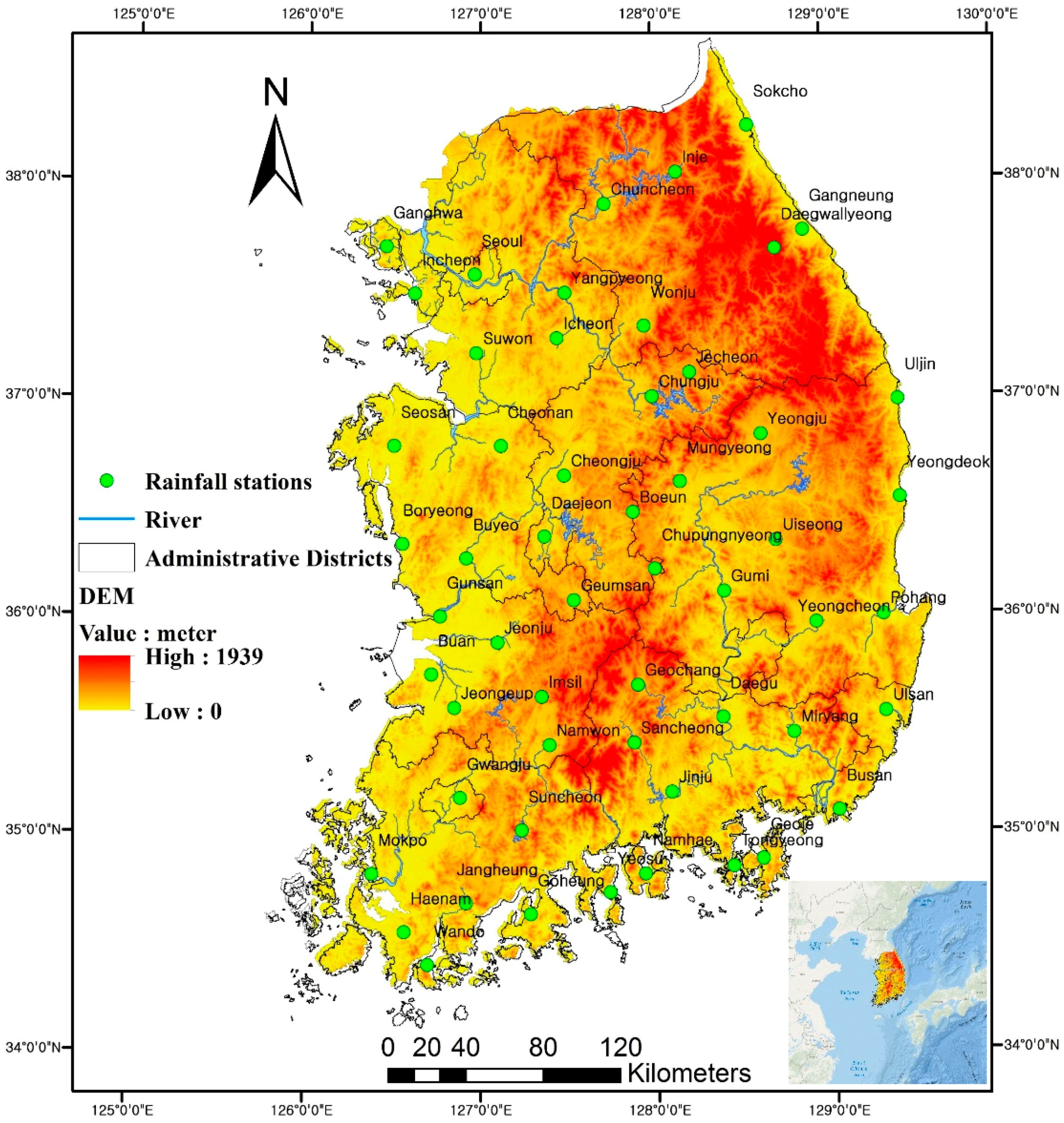
2.1. Study Area and Data

South Korea is located in East Asia and occupies an area equal to 100,210 km². South Korea is heavily affected by the Asian monsoon. Winter consists of dry and cold air masses from the Asian continent, while summer consists of warm and moist air masses from South-Eastern Asia. Figure 1 shows the geographical distribution of the administrative district boundaries, rivers, and topographical characteristics of the 55 rainfall stations used in this study. Initially, monthly precipitation data were collected over 70 rainfall stations maintained by the Korean Meteorological Administration (KMA; web.kma.go.kr) across South Korea. However, only 55 rainfall stations, having the precipitation data from 1980 to 2015 (36 years), were selected, because of non-availability or missing precipitation data at other 15 stations. Initial data analysis for monthly and annual precipitation were performed using the Double Mass method and the Run test to evaluate the homogeneity and randomness of the data, respectively [31].

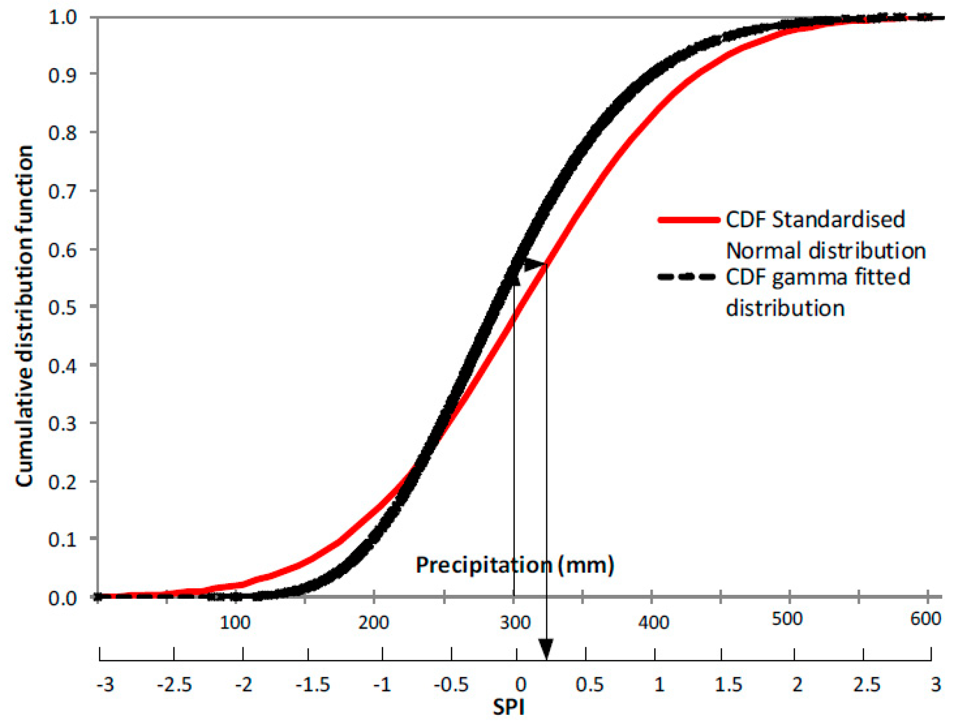
2.2. Standardized Precipitation Index (SPI)

The SPI method proposed by McKee [32] was used to evaluate the drought trends across South Korea. Different SPI timescales (ranges from 1 to 48 months) indicate the effect of drought on the availability of the different water resources. For example, shorter SPI timescales (from 1 to 6 months) indicate the drought index for agriculture practices [32,33], whereas longer SPI timescales (from 12 to 48 months) indicate the drought index for hydrology [33]. In this study, an SPI timescale of 12 months (SPI-12) is used to analyze the spatiotemporal trends across the region. This is because South Korea has more than 18,797 reservoirs across the country, used to supply water for irrigation and manufacturing, and a large number of reservoirs are managed on a timescale of a single year (i.e., reservoirs are filled during the rainy season and drained in the dry season). The SPI time scale is calculated as

$$\mathrm{SPI}=\frac{x_i-\overline{x}}{\sigma }$$

(1)

where $x_i$ indicates the monthly rainfall amount and $\overline{x}$ and $\sigma$ are the mean and standard deviation of rainfall calculated from the whole monthly time series. Since precipitation do not follow the normal distribution, data are transformed to follow a normal distribution. We choose the gamma distribution because it is found that the gamma distribution fit more closely to the precipitation of 55 stations of South Korea [34]. Since there are a number of zero-bounded continuous variables in climatology, it is important to give a distribution that can be used for such variables [35]. Additionally, gamma distribution has been recommended by many researchers for SPI analysis at different time scales across South Korea [36,37].

Finally, the SPI value is calculated by transforming the cumulative probabilities of the Gamma distribution to the standard normal distribution [32,38]. The graph showing the fitness of SPI data is shown in Figure 2.

2.3. Commonly Used Statistical Tests for Trend Detection

2.3.1. Mann-Kendall (MK) Test

The majority of the previous studies assumed that sample data are serially independent. It is known that some hydrometeorological time series such as water quality and streamflow or rainfall time series may show serial correlation. In such cases, the existence of serial correlation will affect the ability of the MK test to assess the significance of trend because the Mann-Kendall and the Theil-Sen are unable to consider the AR(1) process of the time series.

The non-parametric MK test [39,40] is the most widely applied for the detection of trends in a time series. If the total number of data in the time series is indicated by N, then statistic $S$ can be computed as follows;

$$S={\displaystyle \sum }_{i=1}^{N-1}{\displaystyle \sum }_{j=i+1}^{N}sgn\left(Y_j-Y_i\right)$$

(2)

where $Y_j$ indicates the value of the jth data, n indicates the number of data, and $sgn\left(\theta \right)$ is the sign function

$$sgn\left(\theta \right)=\{\begin{array}{cc}+1& if \theta =Y_j-Y_i>0\\ 0& if \theta =Y_j-Y_i=0\\ -1& if \theta =Y_j-Y_i<0\end{array}$$

(3)

The positive (negative) value of $S$ shows the upward (downward) trend. The $S$ is considered to be normally distributed when $N\ge 8$, and its mean and variance can be computed as follows

$$\mathrm{E}\left[S\right]=0$$

(4)

$$\mathrm{var}\left(S\right)=\frac{[N\left(N-1\right)\left(2N+5\right)-{{\displaystyle \sum }}_{i=1}^n{t}_{i}i\left(i-1\right)\left(2i+5\right)]}{18}$$

(5)

where $t_i$ indicates the number of data in the ith tied group. Finally, the standardized test statistics Z can be computed as follows:

$$\mathrm{Z}=\{\begin{array}{ll}\left(S-1\right)/\sqrt{Var\left(S\right)}& S>0\\ 0& S=0\\ \left(S+1\right)/\sqrt{Var\left(S\right)}& S<0\end{array}$$

(6)

A positive value of Z shows an increasing trend, while a negative value shows a decreasing trend. In this study, trends were tested with a significance level of $\mathsf{\alpha }=0.05$. The null hypothesis of no trend is rejected if the absolute value of Z is greater than 1.96.

2.3.2. Theil–Sen’s Estimator

An approach proposed by [41,42] to compute the magnitude of the trend in rainfall time series, which is estimated as follows:

$$\beta =Median\left[Y_i-Y_j/i-j\right] \forall j<i$$

(7)

where $1<j<i<n$. If N is all combinations of record pairs for the entire data set, then value of slope estimates can be $n=N\left(N-1\right)/2$ and $\beta$ is considered to be the median of these n values.

2.3.3. Linear Regression Estimator

The linear regression method is used to estimate the slope. Positive slope value indicates an increasing trend, while a negative value indicates a decreasing trend. The linear regression line can be computed as follows:

$$y=a+bx$$

(8)

where $x$ and y are the explanatory variable and the dependent variable, respectively, while $b$ and $a$ are the slope and intercept, respectively [9].

2.4. Principal Component Analysis (PCA)

PCA uses a dimensional reduction technique to identify the patterns in climatic and meteorological data [43,44,45]. Normalization of the climatic datasets before application of PCA analysis is common practice [4]. However, normalization of the dataset is not required, as long as the data is not excessively skewed [46]. SPI is itself a normalized variable, because the data has previously been transformed using the Gamma distribution. Therefore, there is no need for further normalization of the drought data; nevertheless, normality assessment was made before the application of PCA analysis. Given the drought index (SPI-12) time series at 55 meteorological stations across South Korea, PCA was applied to extract the loading for each meteorological station, as well as scores for each principal component according to covariance matrix and the eigenvalues and eigenvectors. To explore the localized spatial patterns of drought, the rotation of the loadings was performed using the Variance-Max approach to obtain rather independent principal components [47]. The number of leading components retained for rotation was evaluated using the sampling errors of eigenvalues associated with the principal components [48]. In this study, for the SPI-12 time series, only the first four principal components were well separated within the 95% confidence interval. Thus, the spatial variation of drought patterns across South Korea was represented by the four rotated principal components (RPC) score time series. It should be noticed that RPC scores could represent the common time behavior of the SPI-12 time series across the areas with maximum loading [49]. PCA results were used to divide the subregions according to drought characteristics and were used to explore the representative stations while considering the internal spatial variation of drought. Since the topographical and climatic features of South Korea are complex, recognizing the spatial patterns of drought characteristics is the main obstacle for engineers and regional planners. In this study, a 12-month time scale was selected because it could avoid seasonal cycles while retaining the inter-annual variability by the memory effect [49].

2.5. Statistical Tests Considering the Effect of Serial Correlation for Trend Detection

Usually, in trend detection tests, it is assumed that the observed time series is serially independent. However, data such as annual mean or annual maximum precipitation may show significant correlation. In situations when significant serial correlation is present in the time series, the MK test has high chances of showing significant trends, while no trend exists in reality [26,28]. In other words, the existence of serial correlation leads to an increase in the probability of disproportionate rejection of the null hypothesis.

2.5.1. Pre-Whitening (PW)

To reduce the effect of serial correlation, [26,50] proposed pre-whitening of the time series before the application of the trend detection test. This approach has been applied by many researchers for the detection of trends in streamflow [51], precipitation and temperature records [52]. Computation of other time series models could be fitted more closely to the precipitation data [53]; however, the PW approach assumes that time series can be appropriately described by an autoregressive process of order one, AR(1). The PW approach makes it possible to modify the original time series, and apply the trend test on the reduced sample. Modification in the original time series is mainly done by computing the lag-1 serial correlation coefficient ${\widehat{r}}_1$. For a significance level $\mathsf{\alpha }$ if the value of ${\widehat{r}}_1$ is non-significant, then the trend test is applied to the original time series ($y_1, y_2, \dots ,y_n$); otherwise, it is applied to the pre-whitened time series ($y_2-{\widehat{r}}_1{y}_1, y_3-{\widehat{r}}_1{y}_2, \dots ,y_n-{\widehat{r}}_1{y}_{n-1}$).

2.5.2. Trend-Free Pre-Whitening (TFPW)

Removing the AR(1) component from the time series affects the magnitude of the true slope [removal of positive (negative) AR(1) process deflates (inflates) the existing trend] [54]. The TFPW approach is introduced to address this issue [29]. For a given time series, the slope of the trend is estimated through Theil–Sen’s estimator, i.e., Equation (7). Then the original time series is detrended under the assumption of a linear trend and the lag-1 serial correlation coefficient ${\widehat{r}}_1$ is evaluated for the detrended time series. For a significance level $\mathsf{\alpha }$ if the value of ${\widehat{r}}_1$ is non-significant, then the trend test is applied to the original time series; otherwise, the trend test is applied to the detrended pre-whitened series recombined with the initially estimated slope of trend.

2.5.3. Variance Correction (VC) Approach

The VC approach assumes that the N serially correlated observations have the same information as $N^{\ast }(<N)$ uncorrelated observations. Extensive Monte Carlo simulations were performed [29], and it was found that the presence of serial correlation in a given time series does not change the asymptotic normality and mean of the MK test statistic S, but it does change the variance of the distribution of S. The positive (negative) serial correlation leads to an increase (decrease) in the variance of S. Variance of the MK test statistic S can be corrected by using an effective sample size [28,55,56]. The corrected variance of the MK test statistic is given as follows:

$$V{\left(S\right)}^{\ast }=cf\ast V\left(S\right)$$

(9)

$V\left(S\right)$ indicates the variance (dispersion) of the MK test statistic $S$ for the original time series and $cf$ indicates the correction factor as proposed by [56] (represented by $c{f}_1$) and [28] (represented by $c{f}_2$) and can be expressed as follows;

$$c{f}_1=1+\frac{2}{N\left(N-1\right)\left(N-2\right)}{\displaystyle \sum }_{k=1}^{N-1}\left(N-k\right)\left(N-k-1\right)\left(N-K-2\right)r_k^R$$

(10)

and

$$c{f}_2=1+2{\displaystyle \sum }_{k=1}^{N-1}\left(1-k\right)/N)r_k$$

(11)

$r_k^R$ and $r_k$ indicate the ranks and serial correlation coefficient for lag-$k$ of the observed time series data, respectively. In VC approaches, the trend-free time series is constructed using AR(1) ($r_1^R$, $r_1$), which is similar as in the case of the PW and TFPW approaches. Usually, variance correction is performed considering only significant values from all available values of serial correlation coefficients. Additionally, in this study, variance correction is also performed using only the first three serial correlation coefficients (referred to as modMK1 lag-3), as suggested by [57], and using only the first serial correlation coefficient (referred to as modMK2 lag-1) [28]. This flexible formulation of modified tests with the AR(1) assumption for modMK1 and the AR(3) assumption for modMK2 provides the behavior of the statistical test, as it can consider the effect of the finite number of serial correlations on the variance of the MK test statistic S. It is particularly suitable to investigate the effect of increasing number of autocorrelation on the performance of the MK test. $c{f}_1$ and $c{f}_2$ are referred as modMK1 and modMK2, respectively.

The usefulness of the VC approach is obvious, because the lag-1 serial correlation coefficient alone is not sufficient to remove all significant serial correlation in the observed time series [58,59,60]. In order to consider all serial correlations using effective sample size, the modMK1 approach is a better choice for detection of trends in precipitation data. Since the results of modMK1 are comparable with the modMK2, as mentioned by [30], due to length constraints, only the results obtained from modMK1 for precipitation are shown in this study. However, the comparison between the candidate statistical tests is presented for SPI-12 because of the expected strong positive serial correlation in the drought time series.

2.6. Field Significance

The problem of field significance occurs when testing a large number of gauges by simultaneous evaluation of multiple hypotheses [61]. Due to the statistical nature of the tests, there is the possibility of error in the results because of incorrect rejection of the null hypothesis. The significance level 0.05 indicates that in a time series from one gauge there is a 5% chance of identifying a change that does not exist. In most cases, the field significance is calculated using binomial probability distribution, and it is assumed that the cross-correlation (or spatial dependence) between the stations is negligible. However, a bootstrap approach is highly recommended when there is the existence of spatial correlation [62,63]. Field significance was calculated for the AR(1) process and for the test statistics of VC approaches. In the bootstrap methodology, data were sampled simultaneously over the stations to preserve the spatial correlation while removing the temporal correlation and any other possible trend. Each bootstrap testing process started with the testing of the AR(1) process and then different types of Mann-Kendall tests were applied to each series. The time series which was able to pass the tests at a 5% nominal level were noted. The sampling procedure was repeated 10,000 times for defining the sampling distribution, which was further used to set the critical values. A detailed explanation of the bootstrap procedure is provided in [64].

3. Results and Discussion

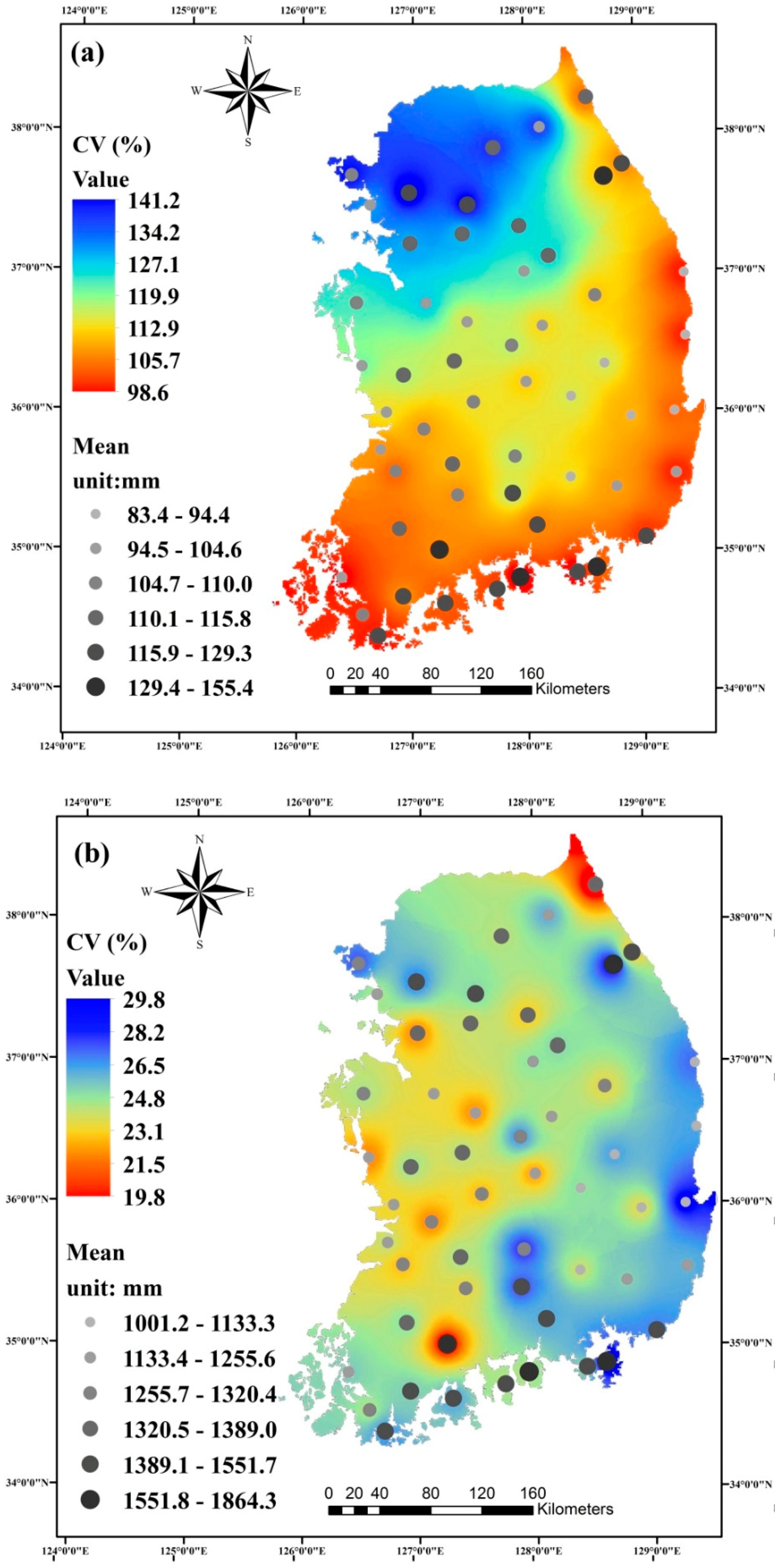
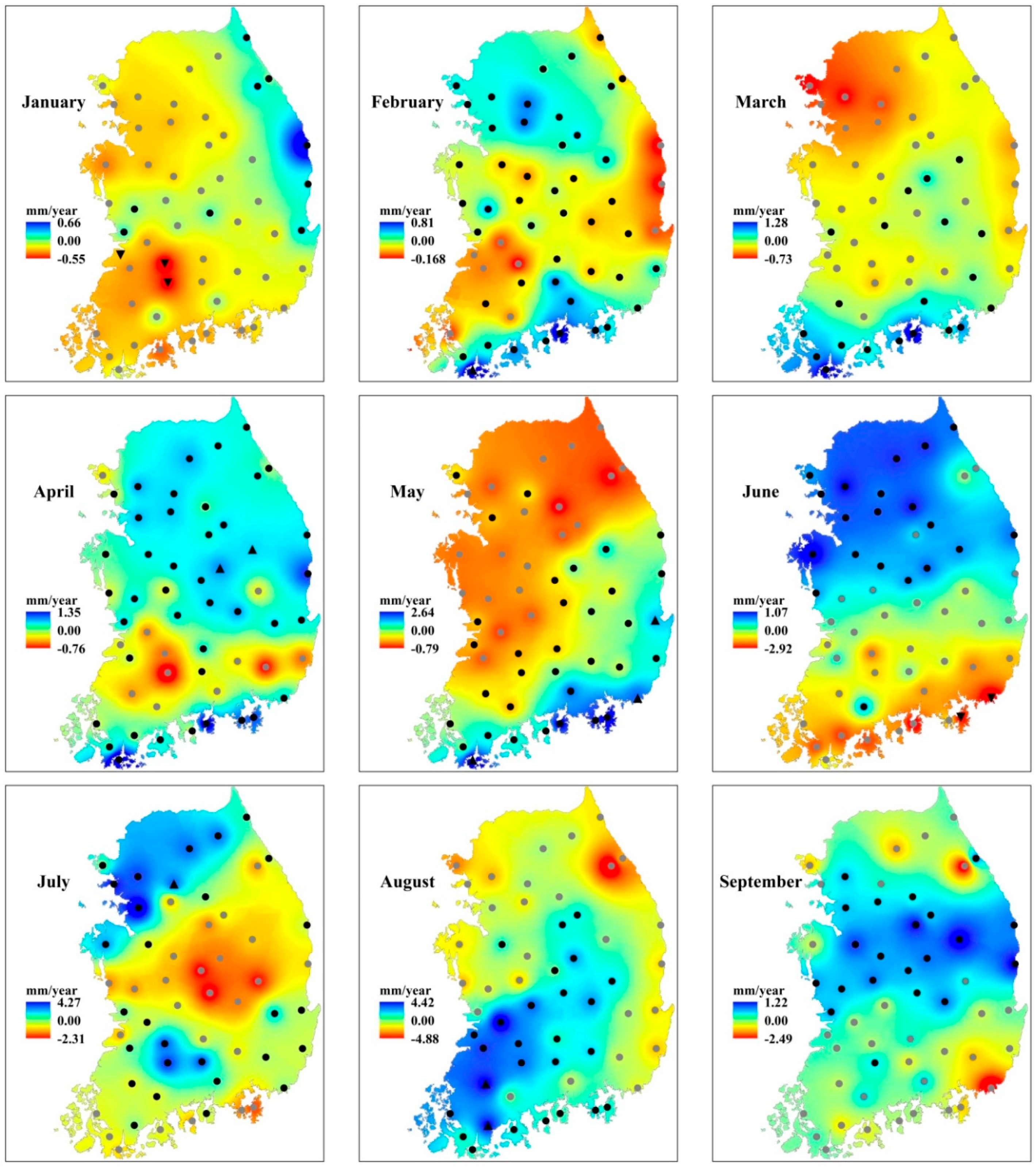
3.1. Spatial Variability of Annual and Monthly Precipitation

The spatial patterns of basic statistical parameters, i.e., mean and coefficient of variation (CV%) for both monthly and annual precipitation from January 1980 to December 2015 at 55 selected meteorological stations are shown in Figure 3. It can be seen that the lowest Monthly Mean Precipitation (MMP), less than 90 mm, occurred at the mid-latitude inland and east coastal areas of South Korea, whereas the highest MMP, greater than 130 mm, occurred at south coast and northern portion of South Korea, Figure 3a. High MMP and Mean Annual Precipitation (MAP) around south coastal areas is because of typhoon-induced changes and convective system within air mass at south coastal areas causing heavy rainfall during summer season [14]. Following the orography, the MMP and MAP increased from all orientations towards the high-altitude areas, as the temperature gets cooler with the increase in altitude. For example, at the top of Seoraksan mountain (located at northeast part of South Korea), it reaches its maximum, with MAP of greater than 1500 mm (Figure 3b). Overall spatial patterns of MAP (Figure 3b) are similar to those of MMP (Figure 3a).

MAP showed moderate spatial variation over a 36-year span, as its CV values vary from 19.8% to 29.8%, with a mean of 24.7%. However, MMP time series (432 months) showed strong variation for different meteorological stations, as CV varies from 98.6% to 141.2%, with a mean value of 113.7%. MAP and MMP showed higher spatial variation along the east and south coast of South Korea, which is due to typhoon-induced changes in precipitation patterns along the coastal areas during monsoon season [14].

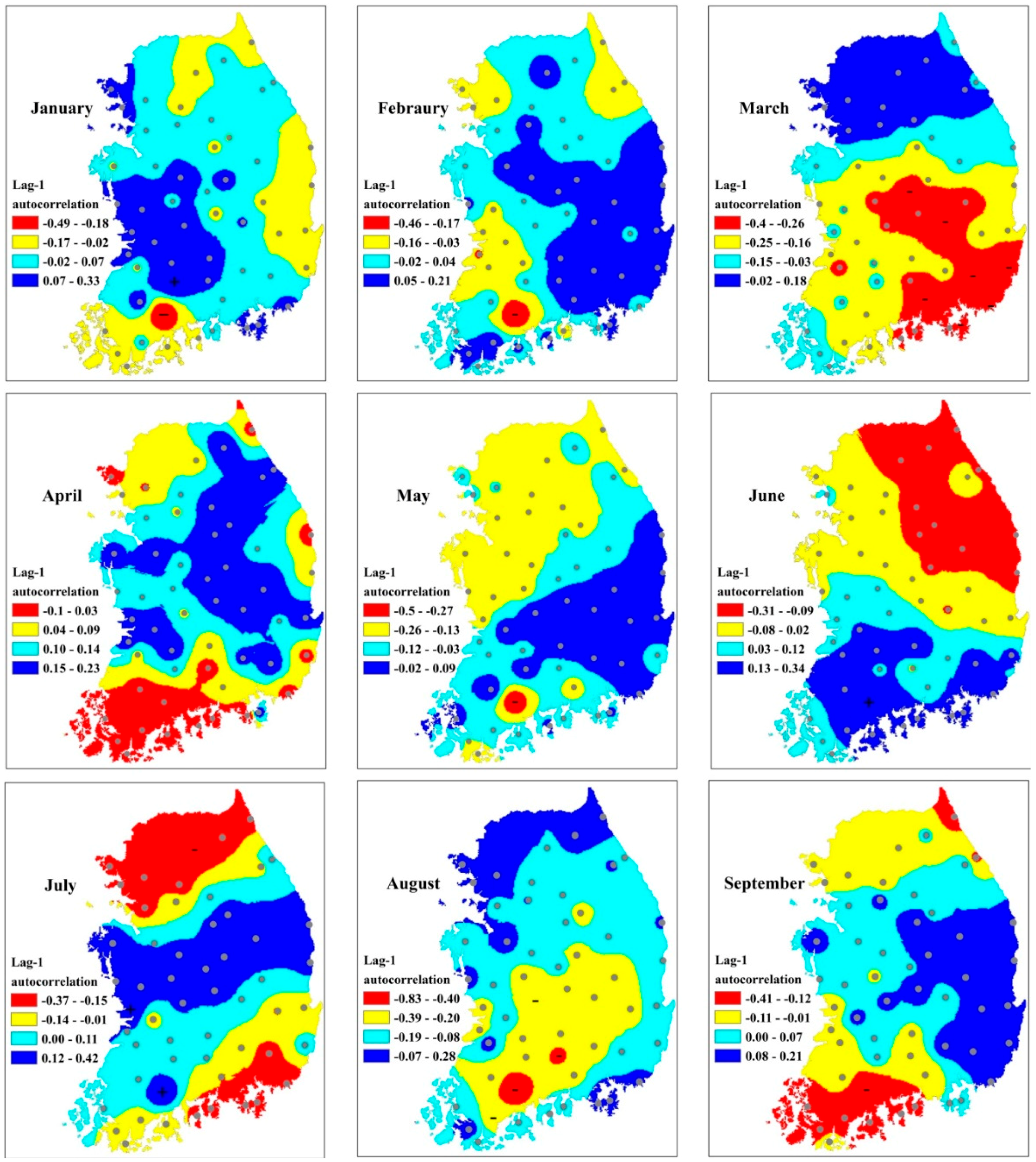
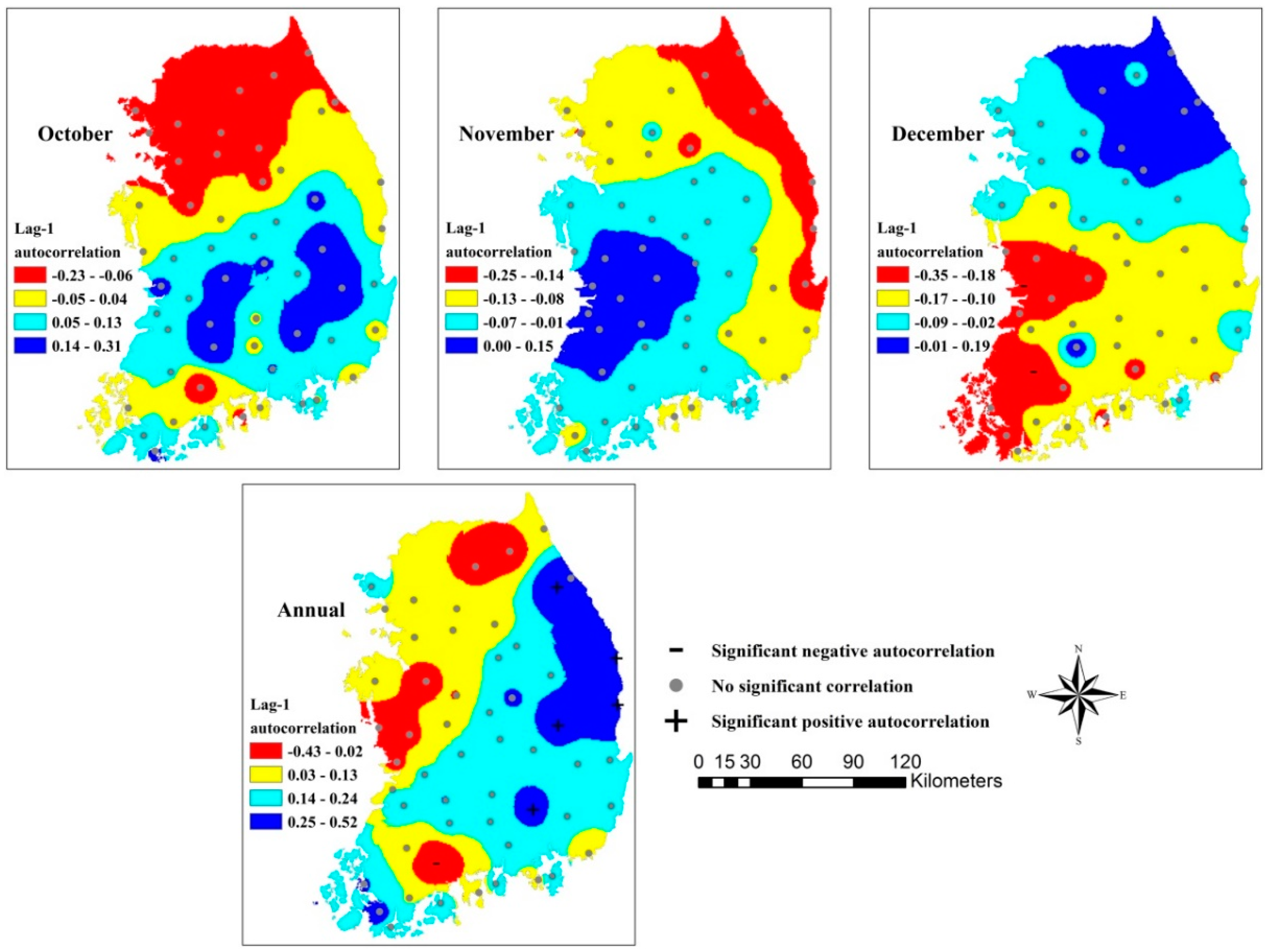
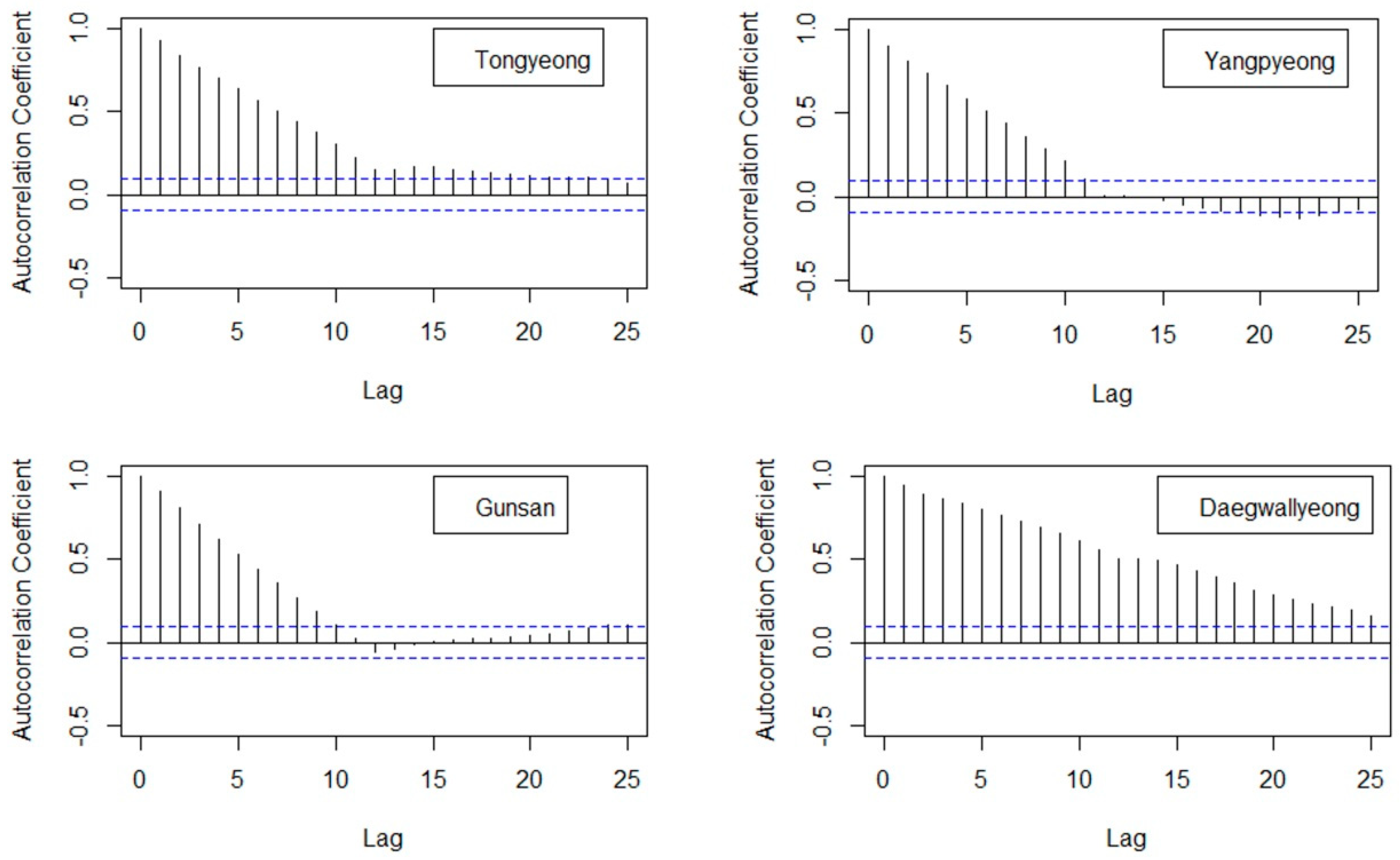
3.2. Autocorrelation of Annual and Monthly Precipitation

The spatial distribution of 55 stations with the interpolated lag-1 significant (positive or negative) autocorrelation coefficient ($r_1$) and non-significant autocorrelation for annual and monthly precipitation data across South Korea is shown in Figure 4. It can be observed that the majority of the stations did not show any significant autocorrelation from January to December. In March almost 12% of the stations (located at southeast coast) and in August only 7% of the stations (located at south coast) showed significant negative autocorrelation. The existence of significant autocorrelation may be because of the existence of spatial dependence or cross-correlation in the time series. To identify the cross-correlation for each pair of stations and for each month, Pearson’s correlation coefficient was calculated. This also helped to evaluate the impact of cross-correlation on field significance. The spatial correlation quantified by Pearson’s correlation showed high values, reaching up to 0.9 during the summer and spring months. The null hypothesis is likely to be rejected too often because of the reduction in the effective sample size. This can be understood as being due to the mechanism whereby when a trend is found at one station it is more likely to find the similar trend at nearby stations [64]. Therefore, there are high chances of showing significant autocorrelation (such as 12% stations in March and 7% stations in August). In April, October and November, none of the stations showed significant autocorrelation. Overall, the number of stations with significant negative autocorrelation (18 stations) is substantially higher than that of significant positive autocorrelation (4 stations). It can be seen that the highest variation in magnitude of lag-1 autocorrelation coefficient was detected during the summer season (June, July and August), while the least variation was observed in the winter season (December, January and February).

For example, the monthly highest lag-1 autocorrelation (0.42) was observed in July precipitation and the monthly lowest (−0.83) was observed in August precipitation. This is because the precipitation characteristics in South Korea are highly influenced by the summer monsoon, known as the “Changma front”, a quasi-stationary front [25]. Extreme changes in the nature of the Changma front in the summer season lead to abrupt changes in the duration and frequency of heavy rainfall [12,25].

In the case of annual precipitation, 9% of the stations (located on the east coast) showed significant positive autocorrelation and 1% of the stations showed significant negative autocorrelation.

Table 1. Summary of the number of stations showing significant and non-significant lag-1 autocorrelation, and significant and non-significant trends across South Korea.

Variable	Significant Autocorrelation		No Significant Autocorrelation	Significant Trends		No Significant Trends
	+	-		Increasing	Decreasing	Increasing	Decreasing
January	1	1	53	0	3	9	43
February	0	1	54	1	0	46	8
March	0	7	48	0	0	20	35
April	0	0	55	2	0	41	12
May	0	1	54	3	0	32	20
June	1	0	54	0	2	20	33
July	2	1	52	1	0	28	26
August	0	4	51	2	0	25	28
September	0	1	54	0	0	21	34
October	0	0	55	1	0	32	22
November	0	0	55	0	0	40	15
December	0	2	53	6	0	41	8
Annual	5	1	49	0	0	38	17

summarizes the number of stations, showing the significant and non-significant lag-1 autocorrelation among 55 stations. It is worthwhile noting that the existence of positive autocorrelation leads to an increase the variance of S, and negative autocorrelation leads to a decrease the variance of S. Thus, for the simple MK test, the positive autocorrelation can increase the false rejection of null hypothesis, and vice versa. Therefore, false rejection rates have been decreased by using corrected variance approach.

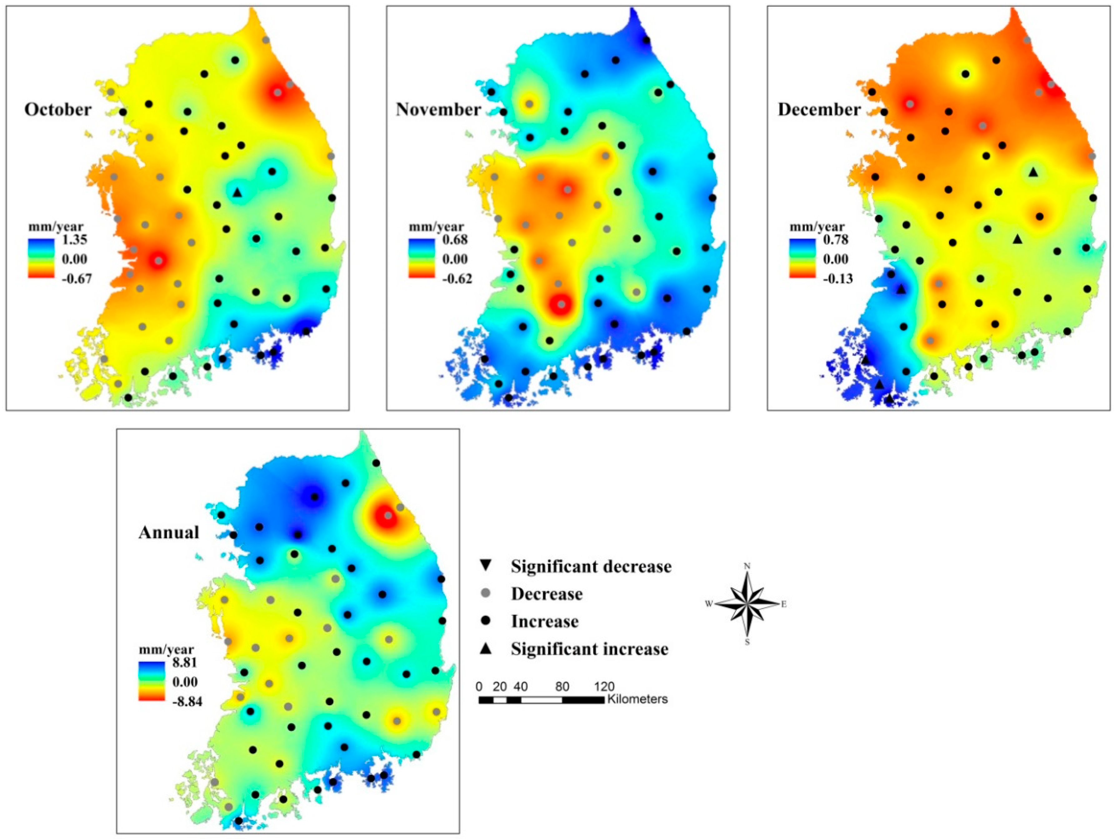
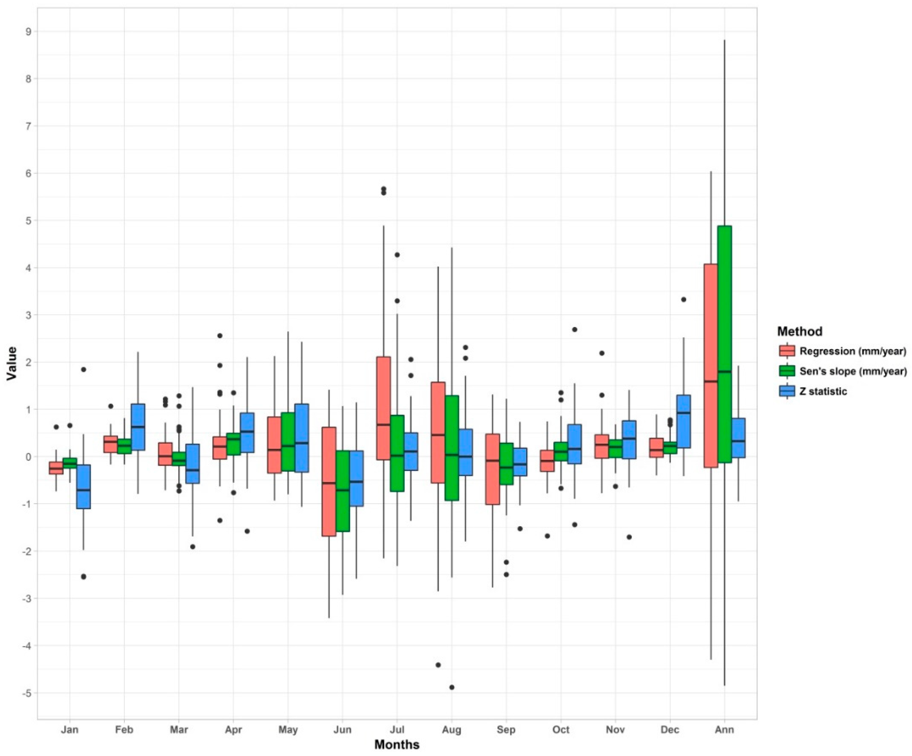
3.3. Spatial Patterns of Temporal Trends in Precipitation

The spatial patterns of the temporal trends in monthly and annual precipitations and their respective magnitudes (in mm/year) were obtained by the modMK1 test, Theil–Sen’s estimator (shown in Figure 5). The value of the Z statistic is divided into four categories to identify the trends; Z < −1.96 indicated a significant decreasing trend, −1.96 < Z < 0 indicated a decreasing trend, 0 < Z < 1.96 indicated an increasing trend and Z > 1.96 indicated a significant increasing trend. Figure 5 shows the changing spatial pattern of the positive (increasing) and negative (decreasing) trends, along with the stations with significant positive and negative trends and their corresponding values of Sen’s slope. The results showed that most of the stations in South Korea were characterized by no significant monthly and annual precipitation trends at the 95% confidence level, as summarized in Table 1. Significant decreasing trends were observed at only three stations (Imsil, Namwon and Buan stations, located in the south west part of South Korea) in January, and two stations (Geoje and Busan stations, located in the south east of South Korea) in June. The highest significant increasing trends were observed at six stations (Yeongju, Gumi, Wando, Haenam, Mokpo, and Jeongeup) in December. No significant trend (neither significant increasing nor significant decreasing) was detected in March, September, November, or annual precipitation. However, when field significance was considered, none of the stations showed trends above the limit of field significance, although December was very close to the limit of field significance. December has the highest number of stations showing significant trends; however, it also had a high limit of field significance. This month is dry throughout the basin, with a baseline of low rainfall punctuated by a few high rainfall years. The spatial patterns of monthly and annual precipitation trends revealed that most of the significant trends (either significant increasing or significant decreasing) were detected along the south coast of South Korea. This is because of the synoptic disturbances, typhoons or convective system within the air mass, leading to extremely unusual precipitation patterns at south coastal areas [14].

In South Korea, more than 50% of the annual precipitation is contributed by summer precipitation (Changma season) and less than 10% is contributed by winter precipitation. Therefore, trends in summer precipitation have a direct impact on trends in annual precipitation. During Changma season, June, July, and August, more than 36%, 50% and 45% of the stations, respectively, showed an increasing trend.

To some extent, these results match those of previous studies [12,13,22] in which summer precipitation trends were studied using a simple Mann-Kendall statistical test [39,40] without considering serial correlation. In the case of [12], the number of stations showing significant trends in summer precipitation was relatively higher than observed in this study. This is because of the existence of serial correlation in the time series, leading to an increase in the number of stations having significant trends, where no trend exists in reality [26,28]. Since this study also deals with serial correlation in the time series, the number of stations with significant trends is relatively less.

The color map represents the magnitude (mm/year) of the trend computed by Theil–Sen’s estimator (Figure 5). It can be seen that the highest variation in the magnitude of the Sen’s slope was detected during the summer season, while the least variation was observed in the winter season. The highest monthly magnitude of the trends was 4.42 mm/year at Jangheung station and the lowest was −4.88 mm/year at Daegwallyeong station, both observed in August precipitation. Overall, the magnitude of the trends increased from January to August and decreased from August to onward. Furthermore, the summer patterns of the Sen’s slope were completely identical to the annual one (increasing trend was observed in the north part in June, north west part in July and south coast in August; annual precipitation also showed an increasing trend in these areas), which indicates the great contribution of summer precipitation to annual precipitation in South Korea. Furthermore, the movement of the increasing trend from the north part (in June and July) to the south part (in August) may be because the coastal areas in southern part of South Korea are vulnerable to the landfall of typhoons in late summer. Reduction in the range of the Sen’s slope in September (1.22 mm/year~−2.49 mm/year) and October (1.36 mm/year~−0.67 mm/year) suggests the intervention of a mixed source of moisture after August. The rainfall in September and October is due to both frontal systems and typhoons.

The localized impact of typhoons may lead to a reduction in the magnitude of trends. Since frontal systems and typhoons are likely to occur simultaneously, it is difficult to separate one from the other. In addition, after August, localized convective or orographically induced precipitation becomes important as the Changma front disappears. Accordingly, complex mountainous terrain across South Korea may lead to different precipitation patterns at adjacent stations.

The box plot of the linear regression, Sen’s slope and Z statistic of the modMK1 is presented in Figure 6 for both monthly and annual time scales. The line drawn within the rectangle and rectangle width in the upper (lower) part of Figure 6 indicates the mean values and 75th (25th) percentile, respectively. The upper and lower ends of the lines indicate the maximum and minimum values, respectively. It can be seen that the monthly and annual trends, as well as the magnitudes computed by the linear regression method, were almost similar to the precipitation trends computed by the modMK1 and Theil–Sen’s estimator in a previous study [65]. Except for in January, March, June and September, monthly precipitation showed positive values of linear regression, Sen’s slope and Z statistics, indicating an increasing trend in most of the selected stations over South Korea. Similarly, for annual precipitation, more than 69% of the stations showed an increasing trend. In addition, an abrupt increase in the range of the maximum, minimum, 75th and 25th percentiles of summer precipitation (Jun, July, and August) was observed for linear regression and Sen’s slope. A sudden increase in trends matches well with previous literature [12,17,18,21,24]. The first possible cause of the increase in the trends in summer precipitation is the Asian Monsoon system, which brings the majority of summer precipitation in a relatively short period [25]. The second possible cause is the sudden increase in the domain-mean geopotential height at 700 hpa (Φ700) over mid-latitude Asia during summer in the mid-1970s [66]. The higher value of geopotential height leads to a stronger northerly wind, producing a moisture convergence and finally producing heavy rainfall over South Korea. Additionally, a recent study has shown that the increase in summer precipitation is linked with the intensification of the upper-level westerly Jet over Korea and the anomalously warm sea surface temperature (SST) in the western North Pacific region [19].

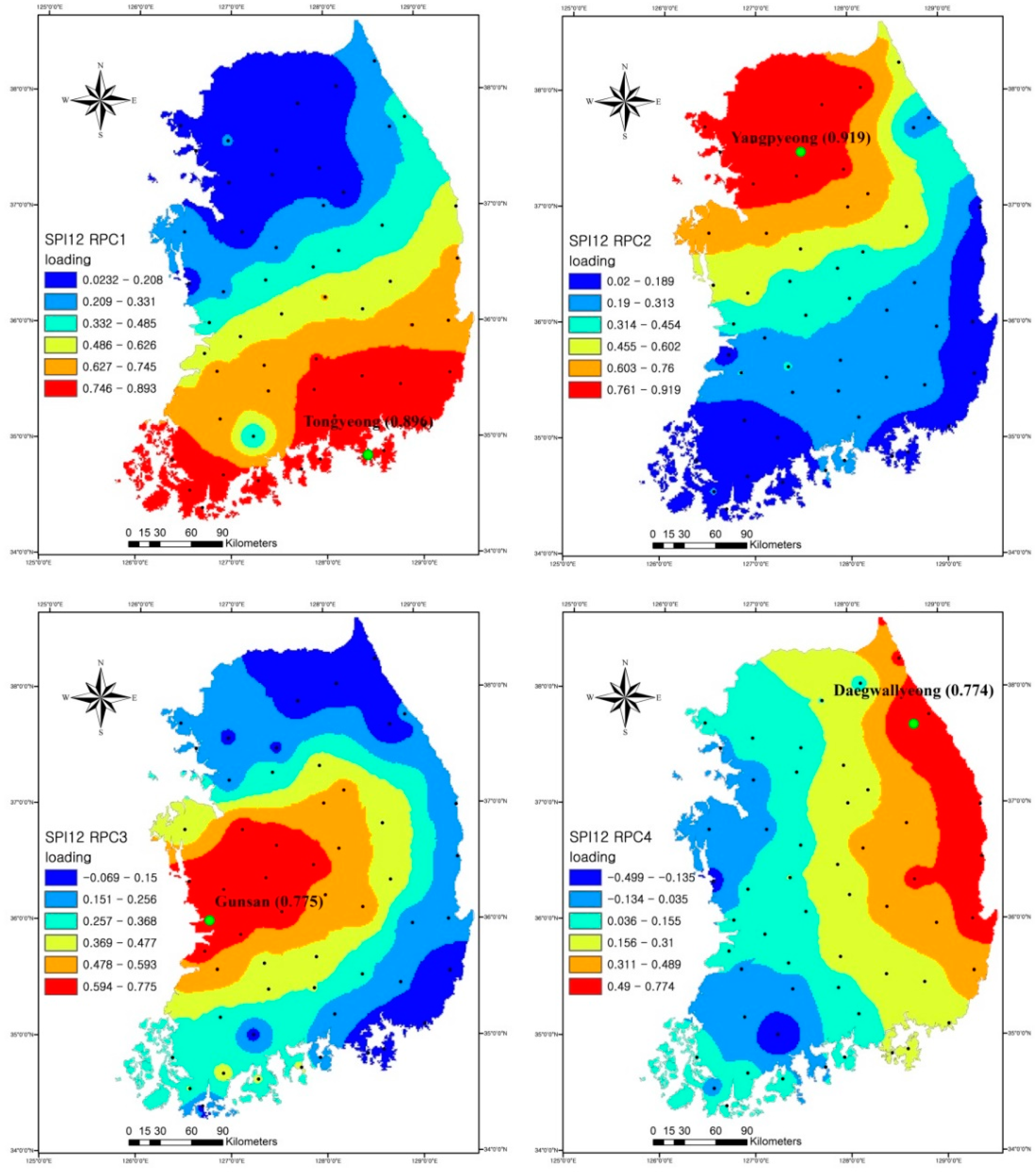
3.4. Spatial Variability of Drought Using PCA

SPI was calculated on a 12-month time scale for 55 meteorological stations to analyze the regional conditions of drought over 432 months from 1980 to 2015. The final result of the PCA applied on SPI-12 time series is presented in

Table 2. Principal component analysis applied on the standardized precipitation index (SPI) for the 55 stations in South Korea.

Principal Components	Eigen Value for Unrotated	% Variance Explained Unrotated	Eigen Value for Rotated	% Variance Explained Rotated
PC1	31.958	58.106	18.628	33.901
PC2	7.753	14.097	12.292	22.3
PC3	3.267	5.940	9.238	16.8
PC4	2.005	3.645	4.826	8.8
Cumulative variance		81.8		81.8

. The percentage of variance explained by the first four un-rotated principal components was 58.11%, 14.11%, 5.94% and 3.65%, respectively, with a cumulative variance of 81.8%. The percentage of variance explained by the first four rotated principal components was 33.89%, 22.31%, 16.78% and 8.82%, respectively. Thus, variance maximum rotation leads to explaining the total variance more evenly using four RPCs, while the cumulative variance (81.80%) is similar to that of the unrotated case.

The rotated loading of the leading four RPCs for drought time series was computed for 55 meteorological stations and interpolated to characterize them by mapping (Figure 7). The leading four RPCs were able to extract approximately 82% of the temporal variation of the drought across the region (Table 2). The spatial distribution of the first RPC (RPC1) indicates the high positive loading along the south coast of South Korea, with a maximum value of 0.896 at Tongyeong station. This shows that south coastal areas had a similar temporal distribution of drought as that detected under the SPI-12 time series. Similarly, the spatial distribution of RPC2, RPC3, and RPC4 indicate the common temporal behavior of drought along the northwest, inland mid-latitude west and east coast of South Korea, with maximum loadings at Yangpyeong (0.919), Gunsan (0.775) and Daegwallyeong (0.774), respectively. Although four RPCs were unable to extract the full temporal variation of drought across the region, their loading seems to divide the whole region into four subregions, characterized by different drought variabilities. This should be related to the variability in seasonal precipitation patterns and orographic effect within the regions. Major regional variability in summer precipitation pattern is due to the gradual movement of the Changma front from south to north [67]. Variability in winter, spring, and autumn precipitation could be mainly due to the orographic effect and variation in ocean water temperature under global warming [68]. The corresponding RPC score time series were also computed for SPI-12 at 55 stations across the region.

RPC scores versus the original SPI-12 time series plotted for four representative stations showed very similar temporal behavior (Figure 8). Since the complex topographical and climatic features of South Korea lead to changes in precipitation patterns from one subregion to another, different temporal patterns and trends of drought were observed at the four representative stations from 1980 to 2015. Extreme drought events were expected to occur in 1994 and 1995 at the south coastal area represented by RPC1, in 1988 and 2015 at the northwest area represented by RPC2, in 1983 and 2003 at the inland mid-latitude west area represented by RPC3, and in 2015 at the east coast area represented by RPC4.

3.5. Spatial Patterns of Temporal Trends in Drought

The autocorrelation coefficients for the four representative stations selected by the PCA approach are shown in Figure 9. The results showed a strong positive and significant serial correlation up to a time lag of approximately 10 months at all representative stations. However, abrupt reduction in the value of the serial correlation coefficient was observed from lag 1 to lag 12. This could be correlated with the inherent computation of SPI at the time scale of 12 months. The maximum lag time for significant serial correlation varied from one station to another. A large number of stations followed a similar trend, in which the acf value was significant up to a time lag of 12 months. The 12-month SPI exhibits some finite moving average properties, where autocorrelation decreases to zero by a certain period, as shown in Figure 8. Depending upon the coefficient in the AR(1) process, a sudden shock in the series may take a very long time to die down, and vice versa. In other words, if a drought lasting many months or even years ends abruptly with 1 or 2 months of intense rainfall. Therefore, the die down period of the autocorrelation coefficient does not necessarily have to be greater than 12 months for SPI-12 [69]. For example, Tongyeong station showed significant and weak serial correlation up to lag 24, while Yangpyeong and Gunsan stations showed significant serial correlations up to time lags of 11 months and 10 months, respectively. It was noticed that autocorrelations were all significant and positive up to a time lag of 7 months for 55 meteorological stations across South Korea. In Serbia [9], it was found that 5 out of 12 stations showed positive autocorrelations in SPI-12 time series at the time lag of 1 month, and the results encouraged the removal of positive autocorrelation to enhance the reliability of the temporal trends identified by the Mann-Kendall test.

Moreover, previous literature has shown that the serial structure of the time series directly affects the ability of trend identification tests to identify trends [28,56,65]. The MK test is not robust against serial correlation [29], sample size, seasonal components and other periodic fluctuations of time series [70]. Therefore, trends in drought series were evaluated using various trend tests, such as modMK1, modMK2, pwMK, and tfpwMK. Every test leads to different results because of differences in their adopted methods to eliminate the effect of serial correlation, which reduces the number of independent observations [60]. There were also greater differences between the tests when field significance was considered. MK, modMK2, modMK2 lag-1 and tfpwMK showed trends above the limit of field significance. Figure 10 shows the changing spatial pattern of the positive (increasing) and negative (decreasing) trends, along with the stations having significant positive and negative trends for each trend test. The box plot in Figure 11 shows the mean, minimum, maximum, 25th and 75th percentile of Z statistic value extracted from each statistical test. The highest number of stations (47%) with significant trends were observed when the original SPI-12 time series data were employed in the MK test (i.e., without considering serial correlation and assuming that data was independent), with the few exceptions for tfpwMK (Figure 10 and

Table 3. Summary of the number of stations with significant and non-significant trends detected by different trend tests for SPI-12 time series across South Korea.

Trend Approach	Significant Trends		No Significant Trends
	Increasing	Decreasing	Increasing	Decreasing
MK	25	1	25	4
modMK1	8	0	42	5
modMK1 lag-3	7	0	43	5
modMK2	19	0	31	5
modMK2 lag-1	16	1	34	4
pwMK	0	0	44	11
tfpwMK	48	2	2	3

). Similarly, the MK test showed an increasing trend with a high mean value of Z statistic (nearly 2), after the tfpwMK test, as shown in Figure 11.

This is because, as compared to independent cases, the trend identification tests tend to show fewer significant trends when the serial structure of time series is taken into account (as all the stations showed a strong positive serial correlation in our study). However, even after considering the effect of serial correlation in the tfpwMK approach, more than 90% of the stations showed significant trends (Figure 10 and Table 3). Furthermore, the highest value of the Z statistic, with a mean greater than 5, confirms the significant increasing trend throughout the region (Figure 11). The possible reason of large number of significant trends as compared to other statistical tests is that the autocorrelation is calculated from trend-free data, leading to the production of a different number of serially correlated time series. Moreover, tfpwMK is unable to consider the effects of higher order dependencies by imposing an AR(1) structure. A study based on the performance of a range of pre-whitening techniques that were developed for the MK test showed flaws in the existing tfpw method [71]. Therefore, as an alternative, they followed the modification based on the idea that the trend residuals are multiplied by a magnification factor for the effective pre-whitening. In case of the pwMK approach, none of the stations showed a significant trend when pre-whitened data were employed (Table 3 and Figure 10). The pwMK test showed the lowest value of the Z statistic, with the mean value nearly equal to 0 (Figure 11).

A possible reason for the smaller number of significant trends is the effect of pre-whitening on the true slope of untransformed SPI-12 time series. This result is in agreement with previous studies [27,30,54]. The smallest number of stations with significant trends was observed for modMK1 lag-3 (12%) and modMK2 lag-1 (30%), as compared to modMK1 (14%) and modMK2 (34%), respectively (Table 3, Figure 10 and Figure 11).

This shows that the finite number of autocorrelation (i.e., without considering high order dependencies) tend to reduce the variance of the MK test statistic S. This observation is in agreement with the findings of a recent study [72]. Overall, the results of the modMK1 and modMK2 are similar because neither of them place any restriction on the number of autocorrelations that can be taken into account and are thus able to handle not only the AR(1) structure but higher-order dependencies.

Overall, the changing spatial patterns of drought severity were almost the same for all trend detection tests. The SPI-12 time series showed a significant decreasing (in the case of MK, modMK2 lag-1, and tfpwMK) or a decreasing (in the case of modMK1, modMK1 lag-3, modMK2) trend at Daegwallyeong station located on the northeast coast, and thus drought severity represented a significant increasing or increasing trend around that region. It is worthwhile to note that similar temporal behavior of drought is also captured by the rotated loading of the fourth principal component (RPC4) with the Daegwallyeong as a representative station, shown in Figure 7. Similarly, increasing trends of drought severity were observed in the surrounding areas of Boryeong (adjacent to Gunsan, which is the representative station of RPC3) and Ulsan (near to Tongyeong which is the representative station of RPC1) station located at inland mid-latitude west and southeast coast, respectively, captured by the RPC3 and RPC1, respectively. Many stations showed significant increasing (in case of MK, modMK1, modMK1 lag-3, modMK2 lag-1 and tfpwMK) or increasing (in case of pwMK) trends in the northwest portion of South Korea (Figure 10), and thus the least severe droughts were observed around this region, as was successfully captured by the RPC2. The results showed that the drought trends detected by various statistical tests approximately matched the results obtained by rotated loadings of the leading four principal components. Exceptions may be because the four RPCs were unable to extract the full temporal variation of drought across the region (approximately 82%, as shown in Table 2).

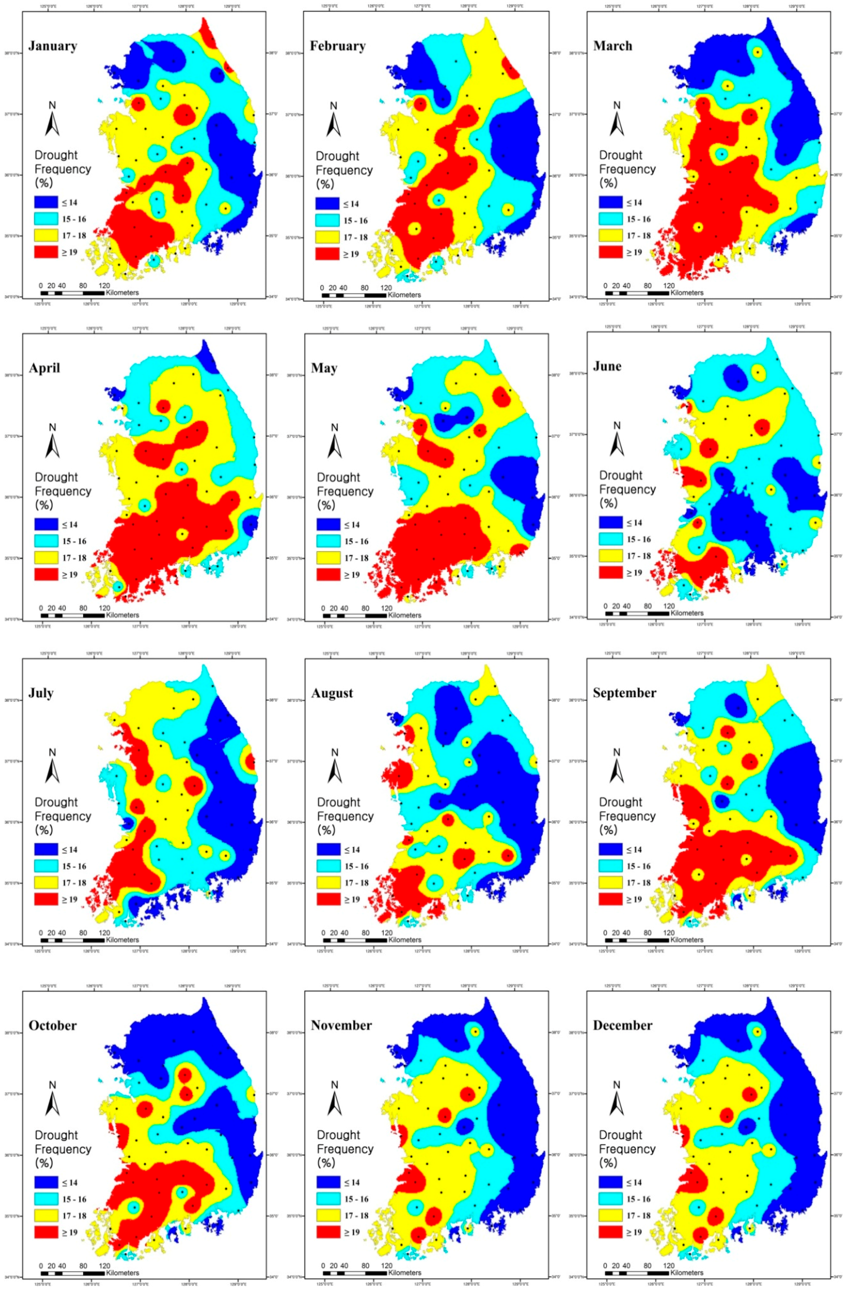
3.6. Spatial Patterns of Drought Frequency

Since droughts vary time and space, the regional distribution of drought using drought events with SPI-12 values less than −1.0 were interpolated and mapped for 12 months in a year. The spatial distribution of relative frequency of drought (%) showed remarkable variation from January to December (Figure 12). Overall, the relative frequency of drought changes according to seasonal variation of precipitation. For example, an almost similar pattern of relative frequency of drought was observed from December to February (winter), from March to May (spring), from June to August (summer) and from September to November (autumn). Throughout the year, the approximate areas with the highest drought frequencies were located on the south west coast of South Korea. Drought events were expected to occur more frequently in the late winter (February), early spring (March and April) and early autumn (September), while droughts were expected to occur least frequently in summer (June, July, August). In February, the areas of high drought frequency expanded from the upper part of south west coast to mid-latitude inland areas, while in March, drought frequency also covered the areas located at west coast. From April to August, the areas of higher drought frequency shrank towards the southwest coast, with a sudden decrease from June. This is because the first peak of the Changma front occurs at the start of June and the second peak occurs at the end of August [19]. A sudden increase in drought frequencies was expected in September around the southwest and south coastal areas because the Changma front disappears in August and non-typhoon precipitation dominates throughout the region. Non-typhoon precipitation is directly affected by the localized convective or orographically induced precipitation.

Moreover, non-typhoon precipitation has a direct connection with the East Atlantic-West Russian teleconnection patterns [73]. The analysis, applied on five major rivers in Korea, confirmed the existence of a correlation between the East Atlantic-West Russian teleconnection patterns and non-typhoon precipitation, and thus influence the hydroclimatic trends over South Korea [14,73,74].

4. Conclusions

In this study, the spatial and temporal variation of rainfall and drought severity were analyzed at 55 stations across South Korea, and the following conclusions were reached:

• The MAP and MMP showed high quantities of rainfall in the north and south part of South Korea, and low quantities in the south coastal areas. High spatial variation of rainfall (CV) was observed on the south coast for MAP and the south and southwest coast for MMP.
• Most of the stations did not show any significant lag-1 serial correlation coefficient for monthly and annual precipitation series, whereas autocorrelations of SPI-12 series were all significant and positive up to a time lag of 7 months for 55 stations across South Korea.
• The spatial patterns of monthly precipitation trends revealed that most of the significant trends were detected along the south coast of South Korea, especially during winter (February, December), late spring (May) and summer (June, August), whereas no significant trend was detected in annual precipitation. The magnitude of the trends increased from January to August and decreased from August onward. Moreover, annual precipitation tends to show similar trends to summer precipitation. When field significance was considered, none of the stations showed trends above the limit of field significance.
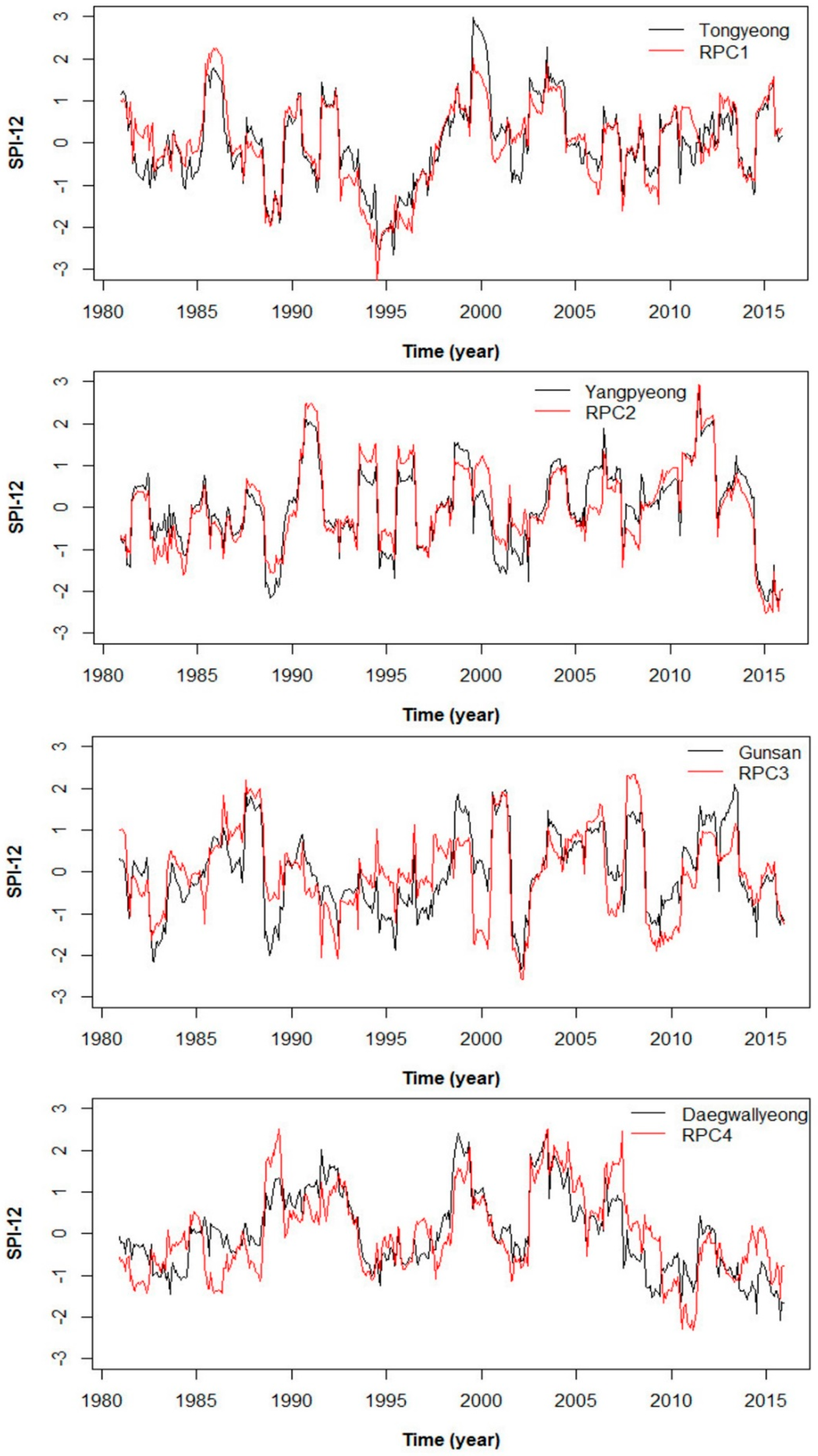
• Principal component analysis applied on SPI-12 series indicated that the whole of South Korea could be divided into four subregions with the different temporal drought behavior, and corresponding representative stations were identified for future drought monitoring.
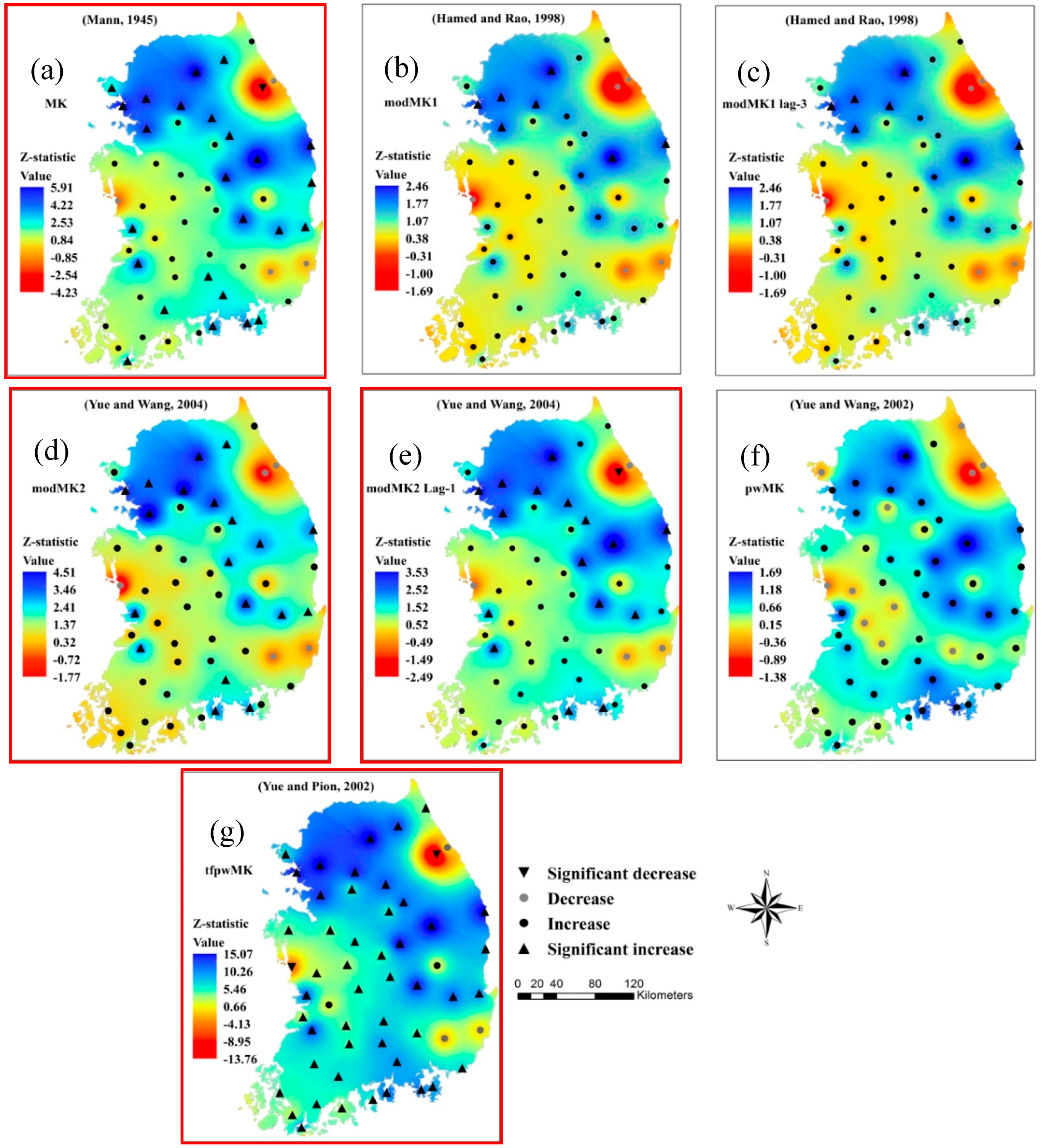
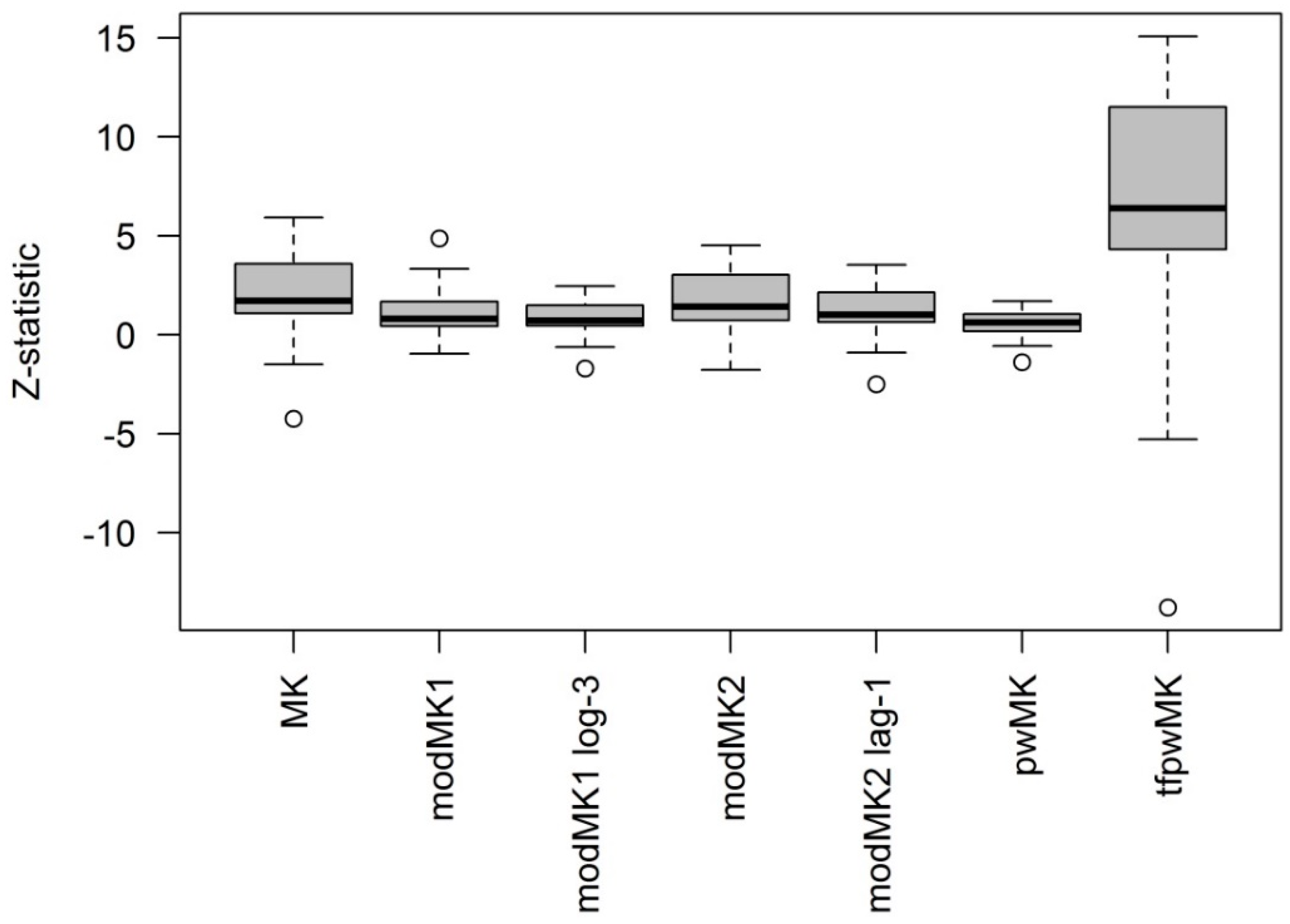
• Removing the serial correlation using the tfpwMK test led to more than 90% of stations having significant trends, which indicates its inability to consider high-order dependencies by imposing the AR(1) structure. Furthermore, the tfpwMK test has serious problems in terms of preserving the nominal significance level. These results match well with previous studies [75]. The pwMK approach showed the lowest value of the Z statistic because of its adverse effect on the true slope of the drought time series. This observation is in agreement with the findings of [76]. VC approaches can handle not only the AR(1) structure, but also higher-order dependencies, and therefore has broader applications. MK, modMK2, modMK2 lag-1 and tfpwMK showed trends above the limit of field significance.
• Trend analysis applied on SPI-12 time series showed significant increasing or increasing trends of drought severity at the stations located at northeast coast, inland mid-latitude west and southeast coastal areas of South Korea. The four representative stations identified by rotated loadings of the leading four principal components were located nearly at the same location.
• Monthly drought frequencies showed that the areas with the highest drought frequencies were in the southwest coastal areas. Drought events were expected to occur more frequently in the late winter, early spring and early autumn, while droughts were expected to occur least frequently in summer.

Overall, increasing trends in summer and annual precipitation with the reduction in drought frequencies in summer suggest the intervention of typhoon-induced precipitation. However, it is difficult to suggest from this study the exact forcing mechanism behind the spatial and temporal trends detected in monthly precipitation and drought time series. As large-scale circulation, global warming, climate change, changes in sea surface temperature in Pacific Ocean and variation in geopotential height might have played an important role, at present, it is difficult to conclude whether the detected trends are related to localized convective and orographical impacts or whether they are a part of decadal variation.

References

1. Paulo, A.A.; Rosa, R.D.; Pereira, L.S. Climate trends and behaviour of drought indices based on precipitation and evapotranspiration in Portugal. Nat. Hazards Earth Syst. Sci. 2012, 12, 1481–1491. [Google Scholar] [CrossRef] [Green Version]
2. Güner Bacanli, Ü. Trend analysis of precipitation and drought in the Aegean region, Turkey. Meteorol. Appl. 2017, 24, 239–249. [Google Scholar] [CrossRef]
3. Azam, M.; Maeng, S.; Kim, H.S.; Murtazaev, A. Copula-Based Stochastic Simulation for Regional Drought Risk Assessment in South Korea. Water 2018, 10, 359. [Google Scholar] [CrossRef]
4. Azam, M.; Park, H.; Maeng, S.J.; Kim, H.S. Regionalization of Drought across South Korea Using Multivariate Methods. Water 2017, 10, 24. [Google Scholar] [CrossRef]
5. Maeng, S.J.; Azam, M.; Kim, H.S.; Hwang, J.H. Analysis of changes in spatio-temporal patterns of drought across South Korea. Water 2017, 9, 679. [Google Scholar] [CrossRef]
6. Azam, M.; Kim, H.S.; Maeng, S.J. Development of flood alert application in Mushim stream watershed Korea. Int. J. Disaster Risk Reduct. 2017, 21, 11–26. [Google Scholar] [CrossRef]
7. Kim, H.S.; Muhammad, A.; Maeng, S.-J. Hydrologic Modeling for Simulation of Rainfall-Runoff at Major Control Points of Geum River Watershed. Procedia Eng. 2016, 154, 504–512. [Google Scholar] [CrossRef]
8. Tabari, H.; Abghari, H.; Hosseinzadeh Talaee, P. Temporal trends and spatial characteristics of drought and rainfall in arid and semiarid regions of Iran. Hydrol. Process. 2012, 26, 3351–3361. [Google Scholar] [CrossRef]
9. Gocic, M.; Trajkovic, S. Analysis of precipitation and drought data in Serbia over the period 1980–2010. J. Hydrol. 2013, 494, 32–42. [Google Scholar] [CrossRef]
10. Zhang, Y.; Cai, W.; Chen, Q.; Yao, Y.; Liu, K. Analysis of changes in precipitation and drought in Aksu River Basin, Northwest China. Adv. Meteorol. 2015, 2015, 215840. [Google Scholar] [CrossRef]
11. Hamed, K.H. Trend detection in hydrologic data: The Mann-Kendall trend test under the scaling hypothesis. J. Hydrol. 2008, 349, 350–363. [Google Scholar] [CrossRef]
12. Chang, H.; Kwon, W.-T. Spatial variations of summer precipitation trends in South Korea, 1973–2005. Environ. Res. Lett. 2007, 2, 45012. [Google Scholar] [CrossRef] [Green Version]
13. Jung, I.W.; Bae, D.H.; Kim, G. Recent trends of mean and extreme precipitation in Korea. Int. J. Climatol. 2011, 31, 359–370. [Google Scholar] [CrossRef]
14. Kim, J.S.; Jain, S. Precipitation trends over the Korean peninsula: Typhoon-induced changes and a typology for characterizing climate-related risk. Environ. Res. Lett. 2011, 6, 034033. [Google Scholar] [CrossRef]
15. Serinaldi, F.; Kilsby, C.G.; Lombardo, F. Untenable nonstationarity: An assessment of the fitness for purpose of trend tests in hydrology. Adv. Water Resour. 2018, 111, 132–155. [Google Scholar] [CrossRef]
16. Clarke, R.T. On the (mis)use of statistical methods in hydro-climatological research. Hydrol. Sci. J. 2010, 55, 139–144. [Google Scholar] [CrossRef] [Green Version]
17. Lee, S.K.W. A variation of summer rainfall in Korea. J. Korean Geogr. Soc. 2004, 39, 819–832. (In Korean) [Google Scholar]
18. Kim, B.J.; Kripalani, R.H.; Oh, J.H.; Moon, S.E. Summer monsoon rainfall patterns over South Korea and associated circulation features. Theor. Appl. Climatol. 2002, 72, 65–74. [Google Scholar] [CrossRef]
19. Baek, H.J.; Kim, M.K.; Kwon, W.T. Observed short- and long-term changes in summer precipitation over South Korea and their links to large-scale circulation anomalies. Int. J. Climatol. 2017, 37, 972–986. [Google Scholar] [CrossRef]
20. Lee, J.J.; Kwon, H.H.; Kim, T.W. Spatio-temporal analysis of extreme precipitation regimes across South Korea and its application to regionalization. J. Hydrol. Environ. Res. 2012, 6, 101–110. [Google Scholar] [CrossRef]
21. Im, E.S.; Jung, I.W.; Bae, D.H. The temporal and spatial structures of recent and future trends in extreme indices over Korea from a regional climate projection. Int. J. Climatol. 2011, 31, 72–86. [Google Scholar] [CrossRef]
22. Bae, D.H.; Jung, I.W.; Chang, H. Long-term trend of precipitation and runoff in Korean river basins. Hydrol. Process. 2008, 22, 2644–2656. [Google Scholar] [CrossRef]
23. Park, J.S.; Kang, H.S.; Lee, Y.S.; Kim, M.K. Changes in the extreme daily rainfall in South Korea. Int. J. Climatol. 2011, 31, 2290–2299. [Google Scholar] [CrossRef]
24. Choi, G.; Kwon, W.-T.; Boo, K.-O.; Cha, Y.-M. Recent Spatial and Temporal Changes in Means and Extreme Events of Temperature and Precipitation across the Republic of Korea. J. Korean Geogr. Soc. 2008, 43, 681–700. [Google Scholar]
25. Chung, Y.-S.; Yoon, M.-B.; Kim, H.-S. On Climate Variations and Changes Observed in South Korea. Clim. Chang. 2004, 66, 151–161. [Google Scholar] [CrossRef]
26. Von Storch, H. Misuses of Statistical Analysis in Climate. In Analysis of Climate Variability; Springer: Berlin/Heidelberg, Germany, 1995; pp. 11–26. [Google Scholar] [CrossRef]
27. Yue, S.; Wang, C.Y. Applicability of prewhitening to eliminate the influence of serial correlation on the Mann-Kendall test. Water Resour. Res. 2002, 38, 4-1–4-7. [Google Scholar] [CrossRef]
28. Yue, S.; Wang, C.Y. The Mann-Kendall test modified by effective sample size to detect trend in serially correlated hydrological series. Water Resour. Manag. 2004, 18, 201–218. [Google Scholar] [CrossRef]
29. Yue, S.; Pilon, P.; Phinney, B.; Cavadias, G. The influence of autocorrelation on the ability to detect trend in hydrological series. Hydrol. Process. 2002, 16, 1807–1829. [Google Scholar] [CrossRef]
30. Khaliq, M.N.; Ouarda, T.B.M.J.; Gachon, P.; Sushama, L.; St-Hilaire, A. Identification of hydrological trends in the presence of serial and cross correlations: A review of selected methods and their application to annual flow regimes of Canadian rivers. J. Hydrol. 2009, 368, 117–130. [Google Scholar] [CrossRef]
31. Adeloye, A.J.; Montaseri, M. Preliminary streamflow data analyses prior to water resources planning study. Hydrol. Sci. 2003, 47, 679–692. [Google Scholar] [CrossRef]
32. Mckee, T.B.; Doesken, N.J.; Kleist, J. The relationship of drought frequency and duration to time scales. In Proceedings of the AMS 8th Conference on Applied Climatology, Anaheim, CA, USA, 17–22 January 1993; pp. 179–184. [Google Scholar]
33. Hayes, M.J.; Svoboda, M.D.; Wilhite, D.A.; Vanyarkho, O.V. Monitoring the 1996 Drought Using the Standardized Precipitation Index. Bull. Am. Meteorol. Soc. 1999, 80, 429–438. [Google Scholar] [CrossRef] [Green Version]
34. Lee, J.H.; Seo, J.W.; Kim, C.J. Analysis on trends, periodicities and frequencies of Korean drought using drought indices. J. Korea Water Resour. Assoc. 2012, 45, 75–89. [Google Scholar] [CrossRef]
35. Thorn, H.C.S. Some methods of climatological analysis. WMO Tech. Note 1966, 81, 16–22. [Google Scholar]
36. Kim, C.J.; Park, M.J.; Lee, J.H. Analysis of climate change impacts on the spatial and frequency patterns of drought using a potential drought hazard mapping approach. Int. J. Climatol. 2014, 34, 61–80. [Google Scholar] [CrossRef]
37. Lee, J.H.; Kim, C.J. A multimodel assessment of the climate change effect on the drought severity-duration-frequency relationship. Hydrol. Process. 2013, 27, 2800–2813. [Google Scholar] [CrossRef]
38. Kao, S.C.; Govindaraju, R.S. A copula-based joint deficit index for droughts. J. Hydrol. 2010, 380, 121–134. [Google Scholar] [CrossRef]
39. Mann, H.B. Nonparametric Tests Against Trend. Econometrica 1945, 13, 245–259. [Google Scholar] [CrossRef]
40. Kendall, M.G. Rank Correlation Methods; Charles Griffin: London, UK, 1975. [Google Scholar]
41. Sen, P.K. Estimates of the Regression Coefficient Based on Kendall’s Tau. J. Am. Stat. Assoc. 1968, 63, 1379–1389. [Google Scholar] [CrossRef]
42. Theil, H. A rank-invariant method of linear and polynomial regression analysis, Part I. Proc. R. Neth. Acad. Sci. 1950, 53, 386–392. [Google Scholar]
43. Singh, P.K.; Kumar, V.; Purohit, R.C.; Kothari, M.; Dashora, P.K. Application of Principal Component Analysis in Grouping Geomorphic Parameters for Hydrologic Modeling. Water Resour. Manag. 2009, 23, 325–339. [Google Scholar] [CrossRef]
44. Kahya, E.; Kalaycı, S.; Piechota, T.C. Streamflow Regionalization : Case Study of Turkey. J. Hydrol. Eng. 2008, 13, 205–214. [Google Scholar] [CrossRef]
45. Raziei, T.; Bordi, I.; Pereira, L.S.; Sutera, A. Space-time variability of hydrological drought and wetness in Iran using NCEP/NCAR and GPCC datasets. Hydrol. Earth Syst. Sci. 2010, 14, 1919–1930. [Google Scholar] [CrossRef] [Green Version]
46. Kalayci, S.; Kahya, E. Assessment of streamflow variability modes in Turkey: 1964–1994. J. Hydrol. 2006, 324, 163–177. [Google Scholar] [CrossRef]
47. Von Storch, H.; Zwiers, F.W. Statistical Analysis in Climate Research. J. Am. Stat. Assoc. 1999, 95, 1375. [Google Scholar] [CrossRef]
48. North, G.R.; Bell, T.L.; Cahalan, R.F. Sampling Errors in the Estimation of Empirical Orthogonal Funtions. Mon. Weather Rev. 1982, 110, 699–706. [Google Scholar] [CrossRef]
49. Raziei, T.; Saghafian, B.; Paulo, A.A.; Pereira, L.S.; Bordi, I. Spatial patterns and temporal variability of drought in Western Iran. Water Resour. Manag. 2009, 23, 439–455. [Google Scholar] [CrossRef]
50. Kulkarni, A.; Von Storch, H. Monte Carlo experiments on the effect of serial correlation on the Mann-Kendall test of trend. Meteorol. Z. 1995, 4, 82–85. [Google Scholar]
51. Zhang, X.; David Harvey, K.; Hogg, W.D.; Yuzyk, T.R. Trends in Canadian streamflow. Water Resour. Res. 2001, 37, 987–998. [Google Scholar] [CrossRef] [Green Version]
52. Zhang, X.; Vincent, L.A.; Hogg, W.D.; Niitsoo, A. Temperature and precipitation trends in Canada during the 20th century. Atmos. Ocean 2000, 38, 395–429. [Google Scholar] [CrossRef] [Green Version]
53. Salas, J. Applied Modeling of Hydrologic Time Series; Water Resources Publication: Littleton, CO, USA, 1980. [Google Scholar]
54. Fleming, S.W.; Clarke, G.K.C. Autoregressive Noise, Deserialization, and Trend Detection and Quantification in Annual River Discharge Time Series. Can. Water Resour. J. 2002, 27, 335–354. [Google Scholar] [CrossRef] [Green Version]
55. Bayley, A.G.V.; Hammersley, J.M.; Supplement, S.; Society, S. The “Effective” Number of Independent Observations in an Autocorrelated Time Series. Suppl. J. R. Stat. Soc. 1946, 8, 184–197. [Google Scholar] [CrossRef]
56. Hamed, K.H.; Ramachandra Rao, A. A modified Mann-Kendall trend test for autocorrelated data. J. Hydrol. 1998, 204, 182–196. [Google Scholar] [CrossRef]
57. Ramachandra Rao, A.; Hamed, K.H.; Chen, H.-L. Nonstationarities in Hydrologic and Environmental Time Series; Springer Science & Business Media: Berlin/Heidelberg, Germany, 2003; Volume 45, ISBN 978-94-010-3979-6. [Google Scholar]
58. Dinpashoh, Y.; Mirabbasi, R.; Jhajharia, D.; Abianeh, H.Z.; Mostafaeipour, A. Effect of Short-Term and Long-Term Persistence on Identification of Temporal Trends. J. Hydrol. Eng. 2014, 19, 617–625. [Google Scholar] [CrossRef]
59. Kumar, S.; Merwade, V.; Kam, J.; Thurner, K. Streamflow trends in Indiana: Effects of long term persistence, precipitation and subsurface drains. J. Hydrol. 2009, 374, 171–183. [Google Scholar] [CrossRef]
60. Sagarika, S.; Kalra, A.; Ahmad, S. Evaluating the effect of persistence on long-term trends and analyzing step changes in streamflows of the continental United States. J. Hydrol. 2014, 517, 36–53. [Google Scholar] [CrossRef]
61. Wilks, D.S. On “field significance” and the false discovery rate. J. Appl. Meteorol. Climatol. 2006, 45, 1181–1189. [Google Scholar] [CrossRef]
62. Yue, S.; Pilon, P.; Phinney, B. Canadian streamflow trend detection: Impacts of serial and cross-correlation. Hydrol. Sci. J. 2003, 48, 51–64. [Google Scholar] [CrossRef]
63. El Kenawy, A.; Lopez-Moreno, J.I.; Vicente-Serrano, S.M. Recent trends in daily temperature extremes over northeastern Spain (1960–2006). Nat. Hazards Earth Syst. Sci. 2011, 11, 2583–2603. [Google Scholar] [CrossRef] [Green Version]
64. Douglas, E.M.; Vogel, R.M.; Kroll, C.N. Trends in floods and low flows in the United States: Impact of spatial correlation. J. Hydrol. 2000, 240, 90–105. [Google Scholar] [CrossRef]
65. Tabari, H.; Talaee, P.H. Temporal variability of precipitation over Iran: 1966–2005. J. Hydrol. 2011, 396, 313–320. [Google Scholar] [CrossRef]
66. Ho, C.H.; Lee, J.Y.; Ahn, M.H.; Lee, H.S. A sudden change in summer rainfall characteristics in Korea during the late 1970s. Int. J. Climatol. 2003, 23, 117–128. [Google Scholar] [CrossRef] [Green Version]
67. Oh, J.-H.; Kwon, W.-T.; Ryoo, S.-B. Review of the researches on Changma and future observational study (KORMEX). Adv. Atmos. Sci. 1997, 14, 207–222. [Google Scholar] [CrossRef]
68. Webster, P.J.; Holland, G.J.; Curry, J.A.; Chang, H.R. Atmospheric science: Changes in tropical cyclone number, duration, and intensity in a warming environment. Science 2005, 309, 1844–1846. [Google Scholar] [CrossRef] [PubMed]
69. Liu, Z.; Wang, Y.; Shao, M.; Jia, X.; Li, X. Spatiotemporal analysis of multiscalar drought characteristics across the Loess Plateau of China. J. Hydrol. 2016, 534, 281–299. [Google Scholar] [CrossRef] [Green Version]
70. Shao, Q.; Li, M. A new trend analysis for seasonal time series with consideration of data dependence. J. Hydrol. 2011, 396, 104–112. [Google Scholar] [CrossRef]
71. Serinaldi, F.; Kilsby, C.G. The importance of prewhitening in change point analysis under persistence. Stoch. Environ. Res. Risk Assess. 2016, 30, 763–777. [Google Scholar] [CrossRef]
72. Tan, X.; Gan, T.Y.; Shao, D. Effects of persistence and large-scale climate anomalies on trends and change points in extreme precipitation of Canada. J. Hydrol. 2017, 550, 453–465. [Google Scholar] [CrossRef]
73. Kim, J.S.; Jain, S.; Moon, Y., II. Atmospheric teleconnection-based conditional streamflow distributions for the Han River and its sub-watersheds in Korea. Int. J. Climatol. 2012, 32, 1466–1474. [Google Scholar] [CrossRef]
74. Kim, J.S.; Jain, S.; Yoon, S.K. Warm season streamflow variability in the Korean Han River Basin: Links with atmospheric teleconnections. Int. J. Climatol. 2012, 32, 635–640. [Google Scholar] [CrossRef]
75. Khaliq, M.N.; Ouarda, T.B.M.J.; Gachon, P. Identification of temporal trends in annual and seasonal low flows occurring in Canadian rivers: The effect of short- and long-term persistence. J. Hydrol. 2009, 369, 183–197. [Google Scholar] [CrossRef]
76. Bayazit, M.; Önöz, B. To prewhiten or not to prewhiten in trend analysis? Hydrol. Sci. J. 2007, 52, 611–624. [Google Scholar] [CrossRef] [Green Version]
Figure 1. Geographical distribution of the administrative district boundaries, rivers, topographical characteristics of the 55 rainfall stations used in this study.
Water 10 00765 g001
Figure 2. The probability transformation from fitted gamma distribution to the standard normal distribution.
Water 10 00765 g002
Figure 3. Mean and Coefficient of variation (CV%) for (a) monthly precipitation (n = 432) and (b) annual precipitation (n = 36) at the 55 selected meteorological stations across the South Korea.
Water 10 00765 g003
Figure 4. Maps showing the spatial patterns of lag-1 autocorrelation coefficient of monthly and annual precipitation across South Korea.
Water 10 00765 g004aWater 10 00765 g004b
Figure 5. Maps showing the spatial patterns of Sen’s slope (mm/year) and Z statistic using modMK1 at 5% significance level for monthly and annual precipitation across South Korea.
Water 10 00765 g005aWater 10 00765 g005b
Figure 6. Values of the slope b of the linear regression, Sen’s slope and Z statistic for monthly and annual precipitation.
Water 10 00765 g006
Figure 7. Spatial variability of rotated loading of the leading four principal components based on principal component analysis applied on drought time series.
Water 10 00765 g007
Figure 8. Temporal patterns of drought time series based on SPI-12 and their corresponding rotated principal component scores at four representative stations from 1980 to 2015.
Water 10 00765 g008
Figure 9. Autocorrelation coefficients of the SPI-12 for the four representative meteorological stations at a critical value α = 0.05.
Water 10 00765 g009
Figure 10. Changing spatial trends of drought severity based on the SPI-12 detected by the (a) regular MK test (without removal of serial correlation), (b) the modified MK (modMK1) test and (c) modified MK test by considering first three lags (modMK1 lag-3) only, (d) the modified MK test (modMK2) and (e) modified MK test considering first lag (modMK2 lag-1) only, (f) pre-whitened MK (pwMK) test and (g) trend-free pre-whitening MK (tfpwMK) test. The number of gauges showing significant trends above the field significance are highlighted in red.
Water 10 00765 g010
Figure 11. Box plot showing the results of the Z statistic for each trend test applied on SPI-12 time series.
Water 10 00765 g011
Figure 12. Spatial distribution of relative frequency of drought (%) based on SPI-12 time series (less than −1) for 55 stations across South Korea.
Water 10 00765 g012