A Semi-Supervised SVM-Firefly Hybrid for Rainfall Estimation from MSG Data

Abstract

In this paper, two improvements in precipitation classification have been performed. Supervised machine learning has demonstrated considerable performances in classification tasks. However, supervised machine learning can only be applied to labeled data. In some cases, large amounts of unlabeled data contain valuable information for better classification. In the classification of precipitation intensities from satellite images, unlabeled data constitute the majority and remain largely unexplored. To exploit both labeled and unlabeled data, a Semi-Supervised Support Vector Machine (S3VM) is implemented as the first improvement for classification results. The labeling of the limited available data is derived from radar measurements covering a small portion of the Meteosat Second Generation Satellite observations. The results show that the S3VM model outperforms the standard SVM model, with up to a 15% improvement in classification accuracy compared to the standard SVM. To achieve the second improvement, the S3VM was combined with the Firefly Algorithm (FFA) to optimize its hyperparameters. This hybridization (S3VM-FFA) enabled an even more robust performance. A comparative study showed that the S3VM-FFA approach yielded highly satisfactory results, achieving a 17% improvement in classification compared to the SVM results. Based on these classifications, precipitation quantities at different scales are estimated. Similarly to the classification results, statistical evaluation parameters indicate that the S3VM-FFA outperforms both the standard SVM and the conventional S3VM.

1. Introduction

In recent years, the planet has experienced climatic instability generating extreme weather phenomena, causing droughts in some regions while others experience floods. The key element for understanding the different situations is the quantities of precipitation that fell. However, measuring these amounts of precipitation is a complex operation due to their great spatial and temporal variability. Traditionally, precipitation is measured using ground-mounted rain gauges. These measurements are very reliable, but they remain specific and not very representative, and complete regions are truncated in this type of measurement. In remote or difficult-to-access areas, direct precipitation measurements are limited. Therefore, remote sensing provides a complementary solution, enabling regional-scale precipitation estimations. Meteorological satellites offer information on cloud cover and the radiometric characteristics of clouds, while weather radars deliver localized and near-instantaneous measurements of precipitation intensity [1,2]. Although these tools do not replace insitu measurements, they help overcome the limitations associated with accessibility and the density of ground station networks.

Satellite observations successfully address major issues regarding coverage and resolution. For two decades, these observations have been used to monitor precipitation, providing a broad spatial coverage and high spatiotemporal resolution. This research leverages data from the Meteosat Second Generation (MSG) Satellite, whose SEVIRI radiometer ensures an adequate spatial and temporal coverage over North Africa for observing precipitation systems. Furthermore, its visible and infrared spectral channels enable the extraction of cloud properties essential for the model. Nonetheless, satellite observations mainly provide indirect signals, particularly cloud-top brightness temperature and reflectance, which must be utilized for estimating precipitation.

Early threshold-based methods for deep convective systems [3,4,5] have evolved into advanced techniques that directly extract cloud microphysical and optical properties from multispectral satellite data [6] for use in precipitation estimation models [7,8,9,10]. In contrast to rain gauges, which provide point-scale measurements and often face issues of sparse spatial coverage, and weather radars that are costly to deploy and maintain, satellite observations offer a continuous and homogeneous coverage over large areas, especially in regions with complex terrain or limited ground infrastructure [11].

Precipitation estimation models are mainly based on supervised machine learning, which has been extensively applied for classifying precipitation intensities. Various approaches have shown effectiveness, including individual classifiers such as neural networks [12], support vector machines [13], random forests [14], and KNNs [15], along with more advanced hybrid models that combine these techniques for a better performance [13]. However, implementing these models requires a labeled dataset, as their effectiveness largely depends on the quality and availability of labeled data. The performance of supervised methods is significantly influenced by this data quality [16]. Insufficient training data can lead to overfitting, where the model memorizes rather than generalizes [17], while poorly labeled data introduces biases that hinder the model’s ability to generalize effectively [18].

Employing unsupervised machine learning to estimate precipitation presents a major challenge. Despite the availability of abundant unlabeled data that provides valuable insights into clouds, the deployment of unsupervised models in this area has not been adequately explored. This lack of thorough examination leads to unstable and fluctuating results [19], a situation aggravated by the absence of established validation criteria for the models [20]. Consequently, this instability greatly diminishes the reliability and performance of these models, thus restricting their effectiveness in estimating precipitation.

To address this, the integration of these two types of data using the concept of semi-supervised models presents an important and promising model due to its ability to exploit labeled and unlabeled data. Machine learning sits between supervised learning, which uses a labeled dataset, and unsupervised learning, which exploits interesting structures in unlabeled data samples.

Based on the foundational theories of semi-supervised learning outlined in landmark studies such as [16], numerous modern algorithms have been developed to address the challenge of limited labeled data across various domains. The works of Song and al.andWang and al. have successfully applied these principles to ship classification and coal sample analysis, respectively [21,22]. Recent advancements in remote sensing and geosciences further demonstrate their effectiveness. For instance, Miao and al. created a multimodal deep graph model for precipitation forecasting [23], while Zhang and al. (2025) introduced a curriculum learning framework for scene classification [24]. Moreover, Hosseiny and al. provide a systematic review of deep learning approaches beyond supervised learning, analyzing semi-supervised, self-supervised, and weakly supervised methods in remote sensing applications [25].

Among classic semi-supervised learning methods, an important family of probabilistic generative models utilizes the Expectation–Maximization (EM) algorithm as a fundamental optimization mechanism [26,27]. These models, such as semi-supervised Gaussian Mixture Models, employ EM to iteratively estimate their parameters based on a mixture of labeled and unlabeled data. This family of generative models represents one of the main categories within the broader taxonomy of semi-supervised techniques.

Graph-based methods use a graph where the nodes are the labeled and unlabeled samples from the dataset. The edges contain the weights associated with the similarities between observations. Each sample transmits its label information to nearby samples until a globally stable state is attained [28]. In semi-supervised learning, co-training methods operate by employing two conditionally independent perspectives of the input data [28,29]. Each perspective trains its own classifier, and the unlabeled samples given the highest confidence by one classifier are used to enhance the labeled set of the other, iteratively refining both models. This model has been broadened to frameworks with multiple classifiers, such as tri-training, which uses three classifiers to create more trustworthy pseudo-labels and reduce the need for strict view independence, thus improving robustness and stability [30]. As for low-density separation methods, they were developed for SVM classifiers that aim to maximize the margin by considering both labeled and unlabeled samples. This category includes transductive SVMs, which minimize the classification error of unlabeled data.

This study focuses on the implementation of the semi-supervised SVM method (S3VM), which makes use of both labeled and unlabeled data. Our contribution utilizes a significant volume of unlabeled data to enhance the supervised learning methodology through gradual integration into the training set. We apply the S3VM model to MSG data to classify precipitation intensities into three categories: convective, stratiform, and non-precipitating. The corresponding rain gauge measurements are employed for data labeling.

To improve the performance of Semi-Supervised Support Vector Machines (S3VMs) and overcome the difficulties of hyperparameter tuning and becoming stuck in local minima, we present a new hybrid approach that combines S3VMs with the Firefly Algorithm (FFA). The FFA, developed by Yang [31], is a robust method known for its success in complex optimization issues [32]. It has already shown promise in optimizing supervised SVMs, leading to more effective classification models [33]. Our goal is to apply this concept to S3VMs, using both labeled and unlabeled data effectively.

The new model, called S3VM-FFA, takes advantage of Firefly’s swarm intelligence to balance between exploring new options and exploiting known good solutions, ensuring a solid performance even with limited labeled data. By applying this optimization strategy, S3VM-FFA achieves a better generalization than traditional methods.

The body of work presented here is organized as follows. Section 2 contains the Study Area and Data. Section 3 details the Methodology, including the mathematical foundations of S3VM and the hybrid optimization algorithms (S3VM-FFA). Section 4 and Section 5 present classification/estimation results and their interpretation. Section 6 concludes with perspectives.

2. Study Area and Data

Precipitation estimates are made in northern Algeria using data from MSG meteorological satellites. We describe the study region and the type of data used for the implementation of our model.

2.1. Study Region

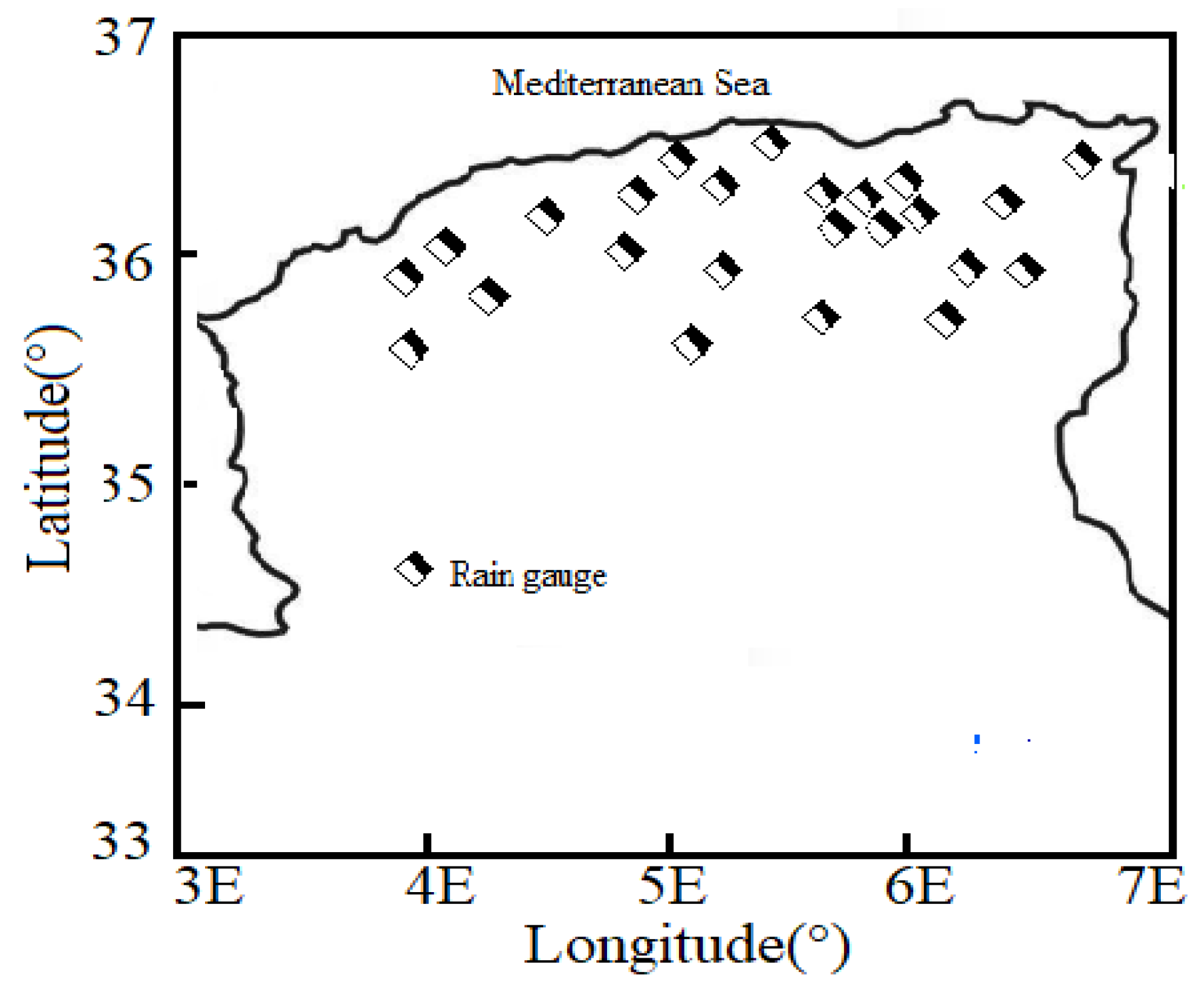
Northern Algeria, located between latitudes 33° and 37°, has a very variable climate (Figure 1). Precipitation rates vary between the north-west, northcentral, and north-east. Northern Algeria experiences different types of precipitation, concentrated mainly during the winter period. They can come from convective systems or stratiform systems; orographic precipitation also occurs due to the mountainous configuration of the region.

2.2. Data

Precipitation can be measured either using rain gauges or through a radar network. MSG data from this region are also available. For the implementation of our model, we considered two types of data: data from the MSG satellite and data from rain gauges. Data collected during the 2009–2010 rainy season are used for training the model. The model was tested considering data from the 2010–2011 rainy seasons.

2.2.1. Rain Gauge Data

Some measurements from rain gauges are used in this study to attempt to construct the labeled data. These measurements taken on an instantaneous scale are reliable but very sparse. We used measurements from rain gauges located in northern Algeria. They consist of 24 measuring stations distributed over the study area (see Figure 1). As stated previously, this data will be used to label some MSG data and for model validation.

The measurements provided by these pluviographs on an instantaneous scale (15 min) are divided into three classes, namely the convective class, stratiform class, and non-precipitating class. The convective class corresponds to measurements that exceed 3.8 mm h⁻¹,while the stratiform class corresponds to measurements less than 3.8 mm h⁻¹.

2.2.2. MSG Data

The input data for our model come from the different channels of the MSG satellite in the form of images. Unlike rain gauge data, this satellite provides a complete and regular coverage of precipitation. In the study region, the spatial resolution reaches 4 × 5 km² depending on the distance from the sub-satellite point. As noted, the time resolution is fifteen minutes. A pixel in each channel is encoded in ten bits, resulting in 1024 different values, called a digital count. Radiances are calculated from these digital counts [34]. The radiances are converted into reflectance in the visible range and into brightness temperature for the water vapor and infrared channels [35]. All MSG satellite channels are two visible (VIS0.6, VIS0.8), one near-infrared (NIR1.6), eight channels between water vapor and infrared (IR3.9, WV6.2, WV7.3, IR8.7, IR9.7, IR10.8, IR12.0, and IR13.4), and ahigh-resolution visible (HRV) channel.

2.2.3. Model Input Attributes

In order to better identify the different types of precipitation, indirect information on optical and microphysical properties and on the thermodynamic phase of clouds is used. Thus, out of the twelve available channels providing brightness temperatures and reflectances, we have selected eight channels, namely VIS0.6, NIR1.6, IR3.9, WV6.2, WV7.3, IR8.7, IR10.8, and IR12. The precipitation intensities contained in clouds can be characterized based on these properties:

• Vertical extension of the clouds (VEC);
• A cloud with a large vertical extension is likely to give significant precipitation rates;
• Temperature of cloud tops (TCT);
• A cloud with a very cold top is a sign of a significant amount of precipitation.

Existence of ice particles in the clouds (EIPC): The presence of ice particles at the tops of clouds is an indicator of low temperature and the maturity of these particles to fall. It corresponds to the thermodynamic phase of clouds.

• Particle size in clouds (PSC);
• Particle size in clouds can indicate whether clouds are precipitating or non-precipitating. Optical thickness of the clouds (OTC): The optical thickness of clouds shows the level of charge by particles in these clouds, and therefore it can indicate whether the cloud is precipitating or non-precipitating.

The different parameters therefore used to extract information on the properties listed above are illustrated in

Table 1. Spectral parameters and corresponding possible values.

Input Parameters	Possible Values		Information About
	Daytime	Nighttime
Τ10.8(Kelvin)	207.2 k to 283.9 k	205.3 k to 282.4 k	VEC and TCT
ΔΤ10.8–12.0(Kelvin)	−0.3 k to 7.4 k	−0.3 k to 7.1 k	EIPC and OTC
ΔT8.7–10.8(Kelvin)	−4.6 k to 1.3 k	−4.8 k to 1.7 k	EIPC
ΔT6.2–10.8(Kelvin)	−50.1 k to 6.4 k	−51.8 k to 5.1 k	VEC
ΔT7.3–12.0(Kelvin)	−50.3 k to 6.6 k	−52.0 k to 5.7 k	VEC and TCT
R0.6 (µm)	0.02 µm to 1 µm	Not used	PSC and OTC
R1.6 (µm)	0.03 µm to 1 µm	Not used	PSC and OTC
ΔT3.9–10.8(Kelvin)	Not used	−10.3 k to 15.1 k	PSC and OTC
ΔT3.9–7.3(Kelvin)	Not used	−4.9 k to 25 k	PSC and OTC

.

It should be noted that the ranges reported in Table 1 represent physically plausible intervals derived from previous studies and validated a posteriori using radar observations over northern Algeria, rather than fixed decision thresholds.

As shown in Table 1, these attributes are used according to their availability. Indeed, certain attributes are used during the day (presence of solar radiation), while other attributes are used during the night (absence of solar radiation). There are also attributes that are used day and night.

The brightness temperature given by IR10.8 is directly linked to the temperature of the cloud tops and therefore to the height of the clouds. This brightness temperature provides information on the vertical extension of clouds [10,35].

The IR10.8 channel combined with the IR12.0 channel can identify non-precipitating cirrus clouds. These non-precipitating clouds with cold tops can be confused with the cumulonimbus clouds with cold, precipitating tops. The ΔT (IR10.8–IR12.0) is a good indicator of OTC, which allows us to separate the cumulonimbus clouds with a large OTC and the cirrus clouds with a weak OTC. The ΔT (IR10.8–IR12.0) is also used to provide information on the presence of ice particles at cloud tops [10].

Water particles and ice particles react differently in the two channels IR8.7 and IR10.8. The absorption is weak between the two wavelengths for water particles, while ice particles show the opposite. Thus, the ΔT (IR8.7–IR10.8) is an indicator of the thermodynamic phase property of the cloud, which corresponds to EIPC [34].

The ΔT (WV6.2–IR10.8) also indicates the VEC. It therefore makes it possible to separate low-level clouds and high-level clouds [9]. With this property, it is possible to provide information on the type of cloud, convective or stratiform.

The ΔT (WV7.3–IR12.0) is used to indicate the EIPC property [14,36]. The absorption is different in the two wavelengths between ice particles and water particles.

The visible channels VIS0.6 and NIR1.6 are used to provide information on the two properties, OTC and PSC, respectively [35,36]. High reflectance values in VIS0.6 correspond to a high OTC. Low reflectance and NIR1.6 values correspond to a high PSC. The two channels in the visible range are used only in the presence of solar radiation.

In the absence of solar radiation, ΔT (IR3.9–IR10.8) and ΔT (IR3.9–WV7.3) are used to deduce information on OTC and PSC [7,33]. The average values of temperature differences correspond to a significant OTC and PSC.

2.2.4. Labeled and Unlabeled Data

The input data for our model are the values of the different attributes presented above, coming from the MSG satellite in the form of images. Thus, for each pixel, a set of attributes is determined. The pixel corresponds to a spatial resolution of 4 × 5 km². 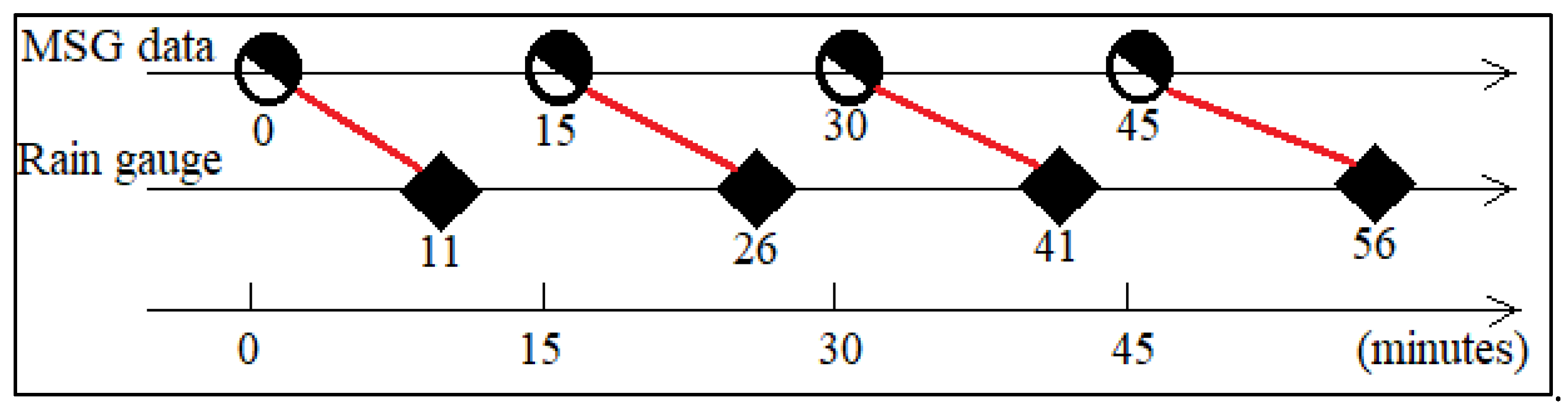To construct a labeled database, we identified the 24 pixels that spatially coincide with the 24 available rainfall stations using their geographic coordinates (see Figure 1). Thus, for each instantaneous observation, 24 pixels are labeled out of the 18,242 making up our study area. The temporal correspondence adopted is illustrated in Figure 2.

The MSG observations at time t coincide with the rain gauge measurements taken at t + 11 min. We assumed that precipitation reaches the ground between 0 and 11 min. The number of labeled pixels and the number of unlabeled pixels during the study period are given in

Table 2. Number of labeled pixels and unlabeled pixels.

	Labeled Data	Unlabeled Data
Learning data	12,532	4,053,120
Validation data	11,923	3,992,011

.

Satellite observations that represent non-cloudy situations are eliminated from the database. They have the same redundant characteristics.

3. Methodology

This study employs a semi-supervised learning model, the S3VM (Semi-Supervised Support Vector Machine), which leverages both labeled and unlabeled data to enhance model generalization.

3.1. Support Vector Machine (SVM)

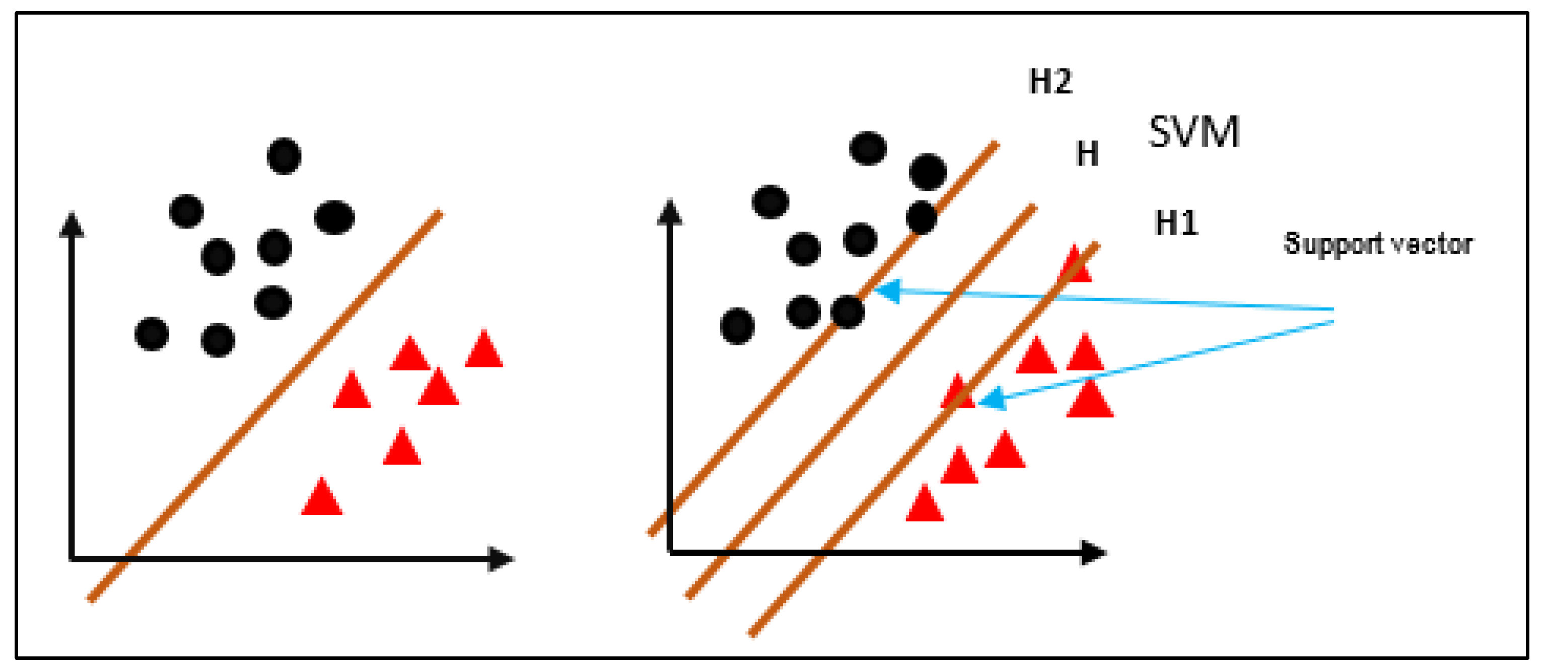
The SVM, introduced by Vapnik [37], is a supervised binary classification algorithm. It identifies a decision function that separates two classes with a maximum margin, utilizing kernel functions for non-linearly separable problems. The complete mathematical formulation is provided in Appendix A.1.

3.2. Semi-Supervised Support Vector Machine (S3VM) Method

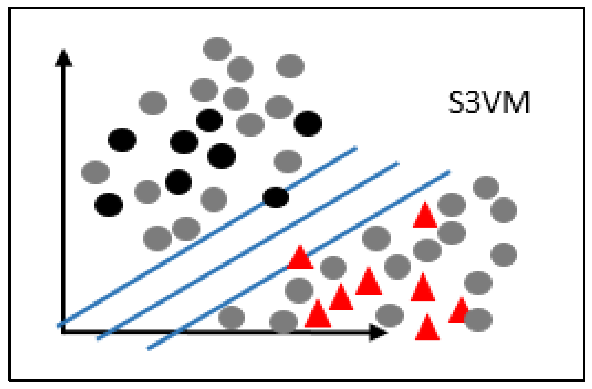
The S3VM method [38] extends this framework to semi-supervised learning. Its objective is to minimize classification error across the entire dataset. Unlabeled data U are integrated through an iterative pseudo-labeling strategy: only samples whose absolute decision function value $\mid f\left(x\right)\mid$ exceeds a confidence threshold, τ, are selected for training. Control mechanisms (excluding uncertain predictions, removing samples with conflicting pseudo-labels between iterations, and halting at convergence) prevent error propagation. A notable variant uses Robust Linear Programming (RLP) with an L1 norm [39].The complete mathematical formulation of the S3VM model is provided in Appendix A.2.

3.3. Learning of the S3VM Model

3.3.1. Cascade Classification Scheme

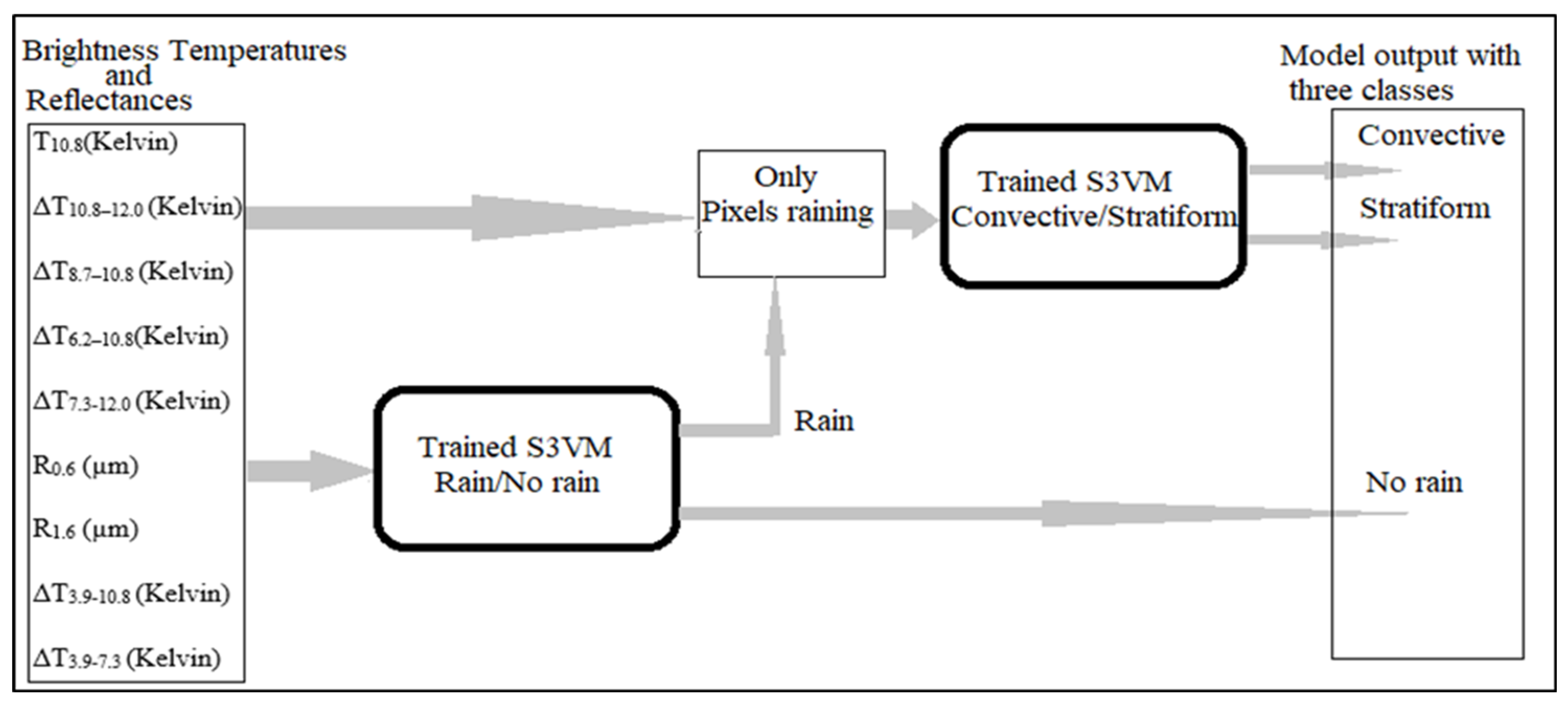
To classify precipitation intensities into three classes, no-rain, stratiform, and convective, a cascade of two binary S3VMs is employed, as depicted in (Figure 3) This approach is necessary because the standard SVM is a binary classifier. The first S3VM (S3VM-1) separates rain pixels (containing both stratiform and convective rain) from no-rain pixels. The second S3VM (S3VM-2) then classifies the rain pixels into stratiform and convective categories.

3.3.2. Input Features and Data Partitioning

The spectral attributes employed for training the models are sourced from MSG channels, offering critical information regarding the microphysical and optical properties of clouds. Acknowledging the fundamental differences in available measurements, particularly the lack of solar reflectance channels at night, two distinct feature sets have been optimized for daytime and nighttime observations.

Table 3. Systematic list of input spectral features for the daytime and nighttime classification models.

Feature Name	Physical Source(MSG Source)	Targeted Cloud Property	Daytime Model	Nighttime Model
TB_10.8	Brightness temperature–IR10.8 µm (atmospheric window channel)	Cloud height (VEC) and temperature (TCT)	✓	✓
BTD_10.8–12.0	ΔT(IR10.8–IR12.0)	Ice phase (EIPC) and optical thickness (OTC)	✓	✓
BTD_8.7–10.8	ΔT(IR8.7–IR10.8)	Ice phase detection (EIPC)	✓	✓
BTD_6.2–10.8	ΔT(WV6.2–IR10.8)	Vertical extent (VEC)	✓	✓
BTD_7.3–12.0	ΔT(WV7.3–IR12.0)	Cloud height and phase (VEC, EIPC)	✓	✓
R_0.6	VIS0.6 µm reflectance	Optical thickness (OTC)	✓
R_1.6	NIR1.6 µm reflectance	Particle size (PSC)	✓
BTD_3.9–10.8	ΔT(IR3.9–IR10.8)	Particle size and optical thickness (PSC, OTC)		✓
BTD_3.9–7.3	ΔT(IR3.9–WV7.3)	Particle size and optical thickness (PSC, OTC)		✓

provides a systematic summary of these input features, outlining their physical origins within MSG channels, the cloud properties they target, and their dedicated use in either daytime or nighttime classifiers. As shown in this table, the daytime model employs eight spectral parameters, while the nighttime model utilizes seven. The derivation and physical interpretation of these spectral parameters are discussed in further detail in Table 1, which also presents their plausible value ranges.

The labeled data comprise 24 pixels that correspond spatially to rain gauge stations (illustrated in Figure 1), while the other pixels throughout the study area are classified as unlabeled data (detailed in Table 2).

3.3.3. Iterative Semi-Supervised Learning Algorithm

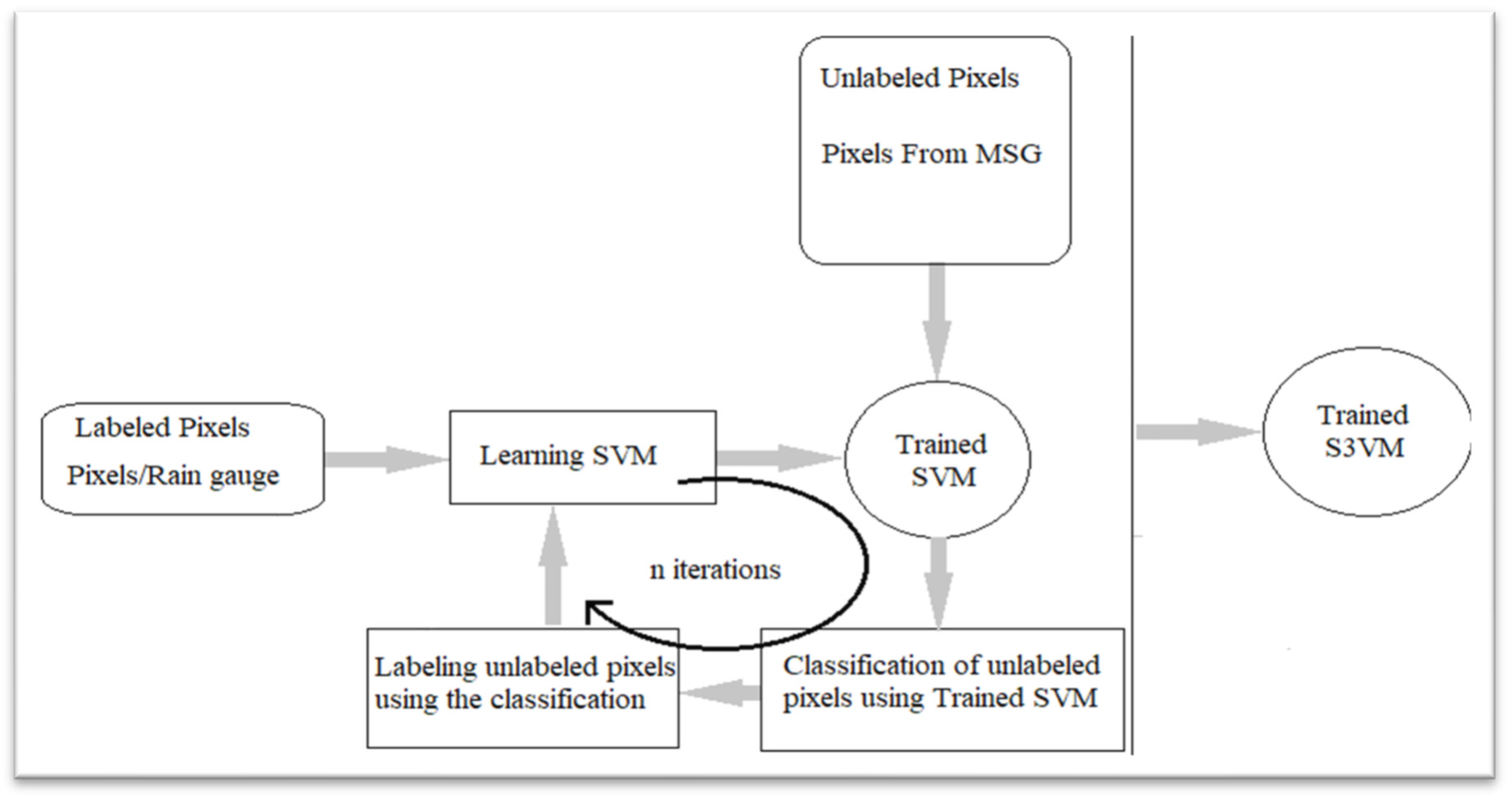
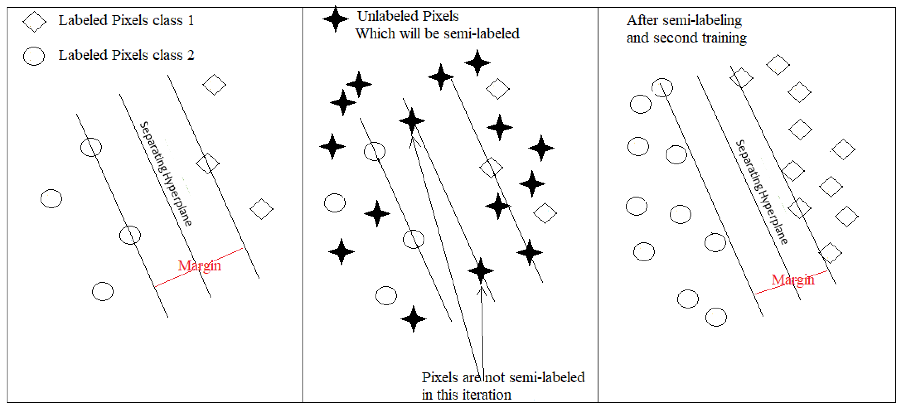
The learning procedure for both S3VM-1 and S3VM-2 follows the same iterative pseudo-labeling strategy (see Figure 4). The process for one iteration is detailed in Figure 5 and operates as follows:

• Initial training: The model is first trained only on the labeled pixels;
• Confident pseudo-labeling: The trained model predicts labels for the unlabeled pixels. Only those unlabeled pixels whose absolute decision function value $\left|f\left(x\right)\right|$ exceeds a confidence threshold $\tau$ are retained as pseudo-labeled samples. Pixels with low confidence (i.e., lying near the decision hyperplane) are kept unlabeled;
• Consistency filtering: To limit error propagation, any pseudo-labeled sample whose assigned label changes between two successive iterations is removed from the training set;
• Model update: The model is retrained on the augmented set containing the original labeled pixels and the filtered pseudo-labeled samples;
• Convergence check: Steps 2–4 are repeated until the decision boundary stabilizes (i.e., the variation between successive iterations becomes negligible).

Figure 4. S3VM training process using labeled pixels and unlabeled pixels.

Figure 4. S3VM training process using labeled pixels and unlabeled pixels.

Figure 5. An iteration encompassing training, semi-labeling and second training.

Figure 5. An iteration encompassing training, semi-labeling and second training.

3.3.4. Daytime and Nighttime Models

As the available spectral features vary between day and night, as systematically presented in Table 3, we constructed two independent cascade classifiers: one designed for daytime observations and another for nighttime observations. Both classifiers operate on the same two-stage classification logic (rain/no rain, followed by stratiform/convective) and follow the iterative semi-supervised learning procedure described above.

3.4. Hybrid S3VM with FFA (S3VM-FFA)

The second enhancement is realized through the novel hybridization of the Semi-Supervised Support Vector Machine (S3VM) and the bio-inspired Firefly Algorithm (FFA) [31]. This method builds upon the standard S3VM framework [16], integrating FFA as an optimizer. The primary objective is to leverage the exploration–exploitation balance inherent in FFA to optimize the hyperparameters of the S3VM, thereby enhancing the classifier’s robustness and ensuring reliable convergence. This hybridization reflects earlier successful applications of Firefly-optimized support vector models in hydrological forecasting, specifically in rainfall prediction [40,41]. While those studies have demonstrated the effectiveness of Firefly-SVM hybrids in supervised settings, our adaptation extends this framework to the semi-supervised context, enabling a more effective utilization of both labeled and unlabeled meteorological data.

3.4.1. Principle of the Bio-Inspired Firefly Algorithm

The Firefly Algorithm (FFA), developed by Xin-She Yang in [31], is a metaheuristic population-based optimization method inspired by the flashing patterns and social behavior of fireflies. In this computational model, fireflies are considered unisex, meaning they are attracted to one another regardless of sex. The attractiveness between fireflies is proportional to their brightness: a less bright firefly will move toward a brighter one. If no brighter firefly is nearby, it will move randomly in the search space.

The algorithm is governed by three main principles:

• All fireflies are unisex;
• Attractiveness is proportional to brightness and decreases with distance;
• The brightness of a firefly is determined by the objective function.

For the complete mathematical formulation and updating rules, please refer to Appendix B.

The Firefly Algorithm (FFA) is chosen for this optimization due to several features that match the needs of S3VM hyperparameter tuning. First, its core mechanism involves attraction based on relative brightness (fitness), which helps balance detailed local searches around good solutions with broader exploration. This is essential for managing the complex, multi-modal loss landscape associated with S3VM. Second, FFA has a simplified parameterization, focusing on the light absorption coefficient (γ) and randomization factor (α). This reduces the likelihood of overfitting on meta-parameters and makes it easier to implement compared to other swarm or evolutionary algorithms. Third, its population-based and parallel structure allows us to efficiently evaluate various hyperparameter sets, which is particularly useful given the high computational costs of training S3VM models. Finally, FFA has shown impressive performance in similar high-dimensional, non-convex optimization tasks within remote sensing [42].

3.4.2. Hybrid S3VM-FFA Approach

The hybridS3VM-FFAapproach we propose aims to enhance the robustness and accuracy of semi-supervised classification by simultaneously addressing its two main challenges: hyperparameter optimization and the risk of convergence to local minima. The core of this method lies in the synergistic coupling of the Semi-Supervised Support Vector Machine (S3VM)model and the metaheuristic Firefly Algorithm (FFA).

The S3VM, governed by the principles outlined in Equations (A12) and (A13), utilizes the geometric structure of unlabeled data to enhance the refinement of the decision boundary. To optimize its critical hyperparameters (notably the regularization coefficients C, γ, and the objective function weights C1, C2), we employ the FFA. Using this technique, each firefly in the swarm represents a set of possible values for these hyperparameters. A firefly’s light intensity (fitness) is evaluated through the classification performance of the S3VM model trained with that configuration on a validation set. The algorithm then proceeds iteratively, where fireflies are attracted toward the best-performing configurations (exploitation), while a stochastic component, controlled by the parameter α in Equation (A22), ensures a continuous exploration of the search space. This mechanism not only identifies a near-optimal hyperparameter configuration globally but also avoids the pitfalls of local optima. The final model, S3VM-FFA, is therefore an S3VM whose architecture has been robustly and automatically optimized by the swarm intelligence of the FFA, leading to an improved generalization for the task of precipitation classification from satellite data. This integrated S3VM-FFA framework is operationalized by the algorithm presented in Appendix B.

For each precipitation class (i), a binary confusion matrix is constructed following a one-versus-rest strategy. In this context, “class (i)” refers to pixels belonging to the target class, while “no class (i)” denotes pixels belonging to any of the remaining classes. Therefore, “no class (i)” does not indicate unclassified pixels, but rather pixels assigned to classes other than class (i).

• The values of the confusion matrix, True Positives (TPs), False Positives (FPs), False Negatives (FNs), and True Negatives (TNs), are determined by comparing the model’s classification outputs with the ground-truth measurements from the 24 rain gauge stations. For each satellite pixel that spatially coincides with a rain gauge station, we compare the class predicted by the model (convective, stratiform, or no rain) with the actual class recorded by the gauge. This one-to-one comparison is illustrated in Table 4.
• True Positives (TPs): Pixels correctly classified as belonging to class I;
• False Positives (FPs): Pixels incorrectly classified as class i (true non-i);
• False Negatives (FNs): Pixels incorrectly classified as non-I (true class i);
• True Negatives (TNs): Pixels correctly classified as non-I;
• n: Total number of validated pixels (n = TP + FP + FN + TN).

These values are then used to compute the performance metrics (POD, FAR, CSI, PC, etc.) as defined in Equations (1)–(6).

A detailed analysis of classification performance for convective precipitation detection is provided by the model-specific confusion matrices in Table 4, Table 5 and Table 6. These matrices quantify the type and frequency of errors for each classifier.

Table 4. Confusion matrix.

	Measured by Rain Gauges
Classified by Developed Model		Class (i)	No Class (i)	Total
	Class (i)	TP	FP	TP+ FP
	No Class (i)	FN	TN	FN + TN
	Total	TP + FN	FN + TN	TP + FP + FN + TN = n

Table 4. Confusion matrix.

	Measured by Rain Gauges
Classified by Developed Model		Class (i)	No Class (i)	Total
	Class (i)	TP	FP	TP+ FP
	No Class (i)	FN	TN	FN + TN
	Total	TP + FN	FN + TN	TP + FP + FN + TN = n

Table 5. Confusion matrix for the SVM model (convective vs. non-convective classification).

	Measured by Rain Gauges
Predicted by SVM Model		Convective	No Convective	Total
	Convective	1896	1374	3270
	No Convective	535	8119	8654
	Total	2431	9493	11,923

Table 5. Confusion matrix for the SVM model (convective vs. non-convective classification).

	Measured by Rain Gauges
Predicted by SVM Model		Convective	No Convective	Total
	Convective	1896	1374	3270
	No Convective	535	8119	8654
	Total	2431	9493	11,923

Table 6. Confusion matrix for the S3VM model (convective vs. non-convective classification).

	Measured by Rain Gauges
Predicted by S3VM Model		Convective	No Convective	Total
	Convective	1130	484	1614
	No Convective	112	10,197	10,309
	Total	1242	10,681	11,923

Table 6. Confusion matrix for the S3VM model (convective vs. non-convective classification).

	Measured by Rain Gauges
Predicted by S3VM Model		Convective	No Convective	Total
	Convective	1130	484	1614
	No Convective	112	10,197	10,309
	Total	1242	10,681	11,923

A comparative analysis of the confusion matrices for convective precipitation (Table 4, Table 5 and Table 6) provides a clear, quantitative narrative of model improvement. The standard SVM (Table 5) exhibits a critical weakness: a high propensity for false alarms, with 1374 False Positives (FPs). While it successfully detects many events (1896 True Positives), its low precision limits operational reliability. The introduction of semi-supervised learning (S3VM, Table 6) addresses this flaw decisively, reducing false alarms by 65% (FP = 484). This leap in precision is achieved by leveraging the geometric information within the abundant unlabeled data to find a more generalizable decision boundary.

The final S3VM-FFA model (

Table 7. Confusion matrix for the S3VM-FFA model (convective vs. non-convective classification).

	Measured by Rain Gauges
Predicted by S3VM-FFA Model		Convective	No Convective	Total
	Convective	1028	400	1428
	No Convective	77	10,418	10,495
	Total	1105	10,818	11,923

), optimized via the Firefly Algorithm, refines this boundary further. It achieves the most robust performance by simultaneously minimizing both types of classification errors: it yields the lowest counts of both False Positives (FP = 400) and False Negatives (FN = 77). Consequently, it attains the highest number of True Negatives (TN = 10,418), indicating a superior specificity. This balanced improvement, capturing more true events while generating fewer false alerts, is the quantitative signature of a successfully optimized classifier. The progression from SVM to S3VM to S3VM-FFA, as evidenced by these matrices, confirms that the hybrid approach effectively translates metaheuristic optimization into tangible gains in classification accuracy and operational trustworthiness.

4. Application and Results

We implemented the S3VM-FFA model on the MSG dataset collected during the 2010/2011 rainy season. To demonstrate the contribution of the S3VM-FFA model compared to the isolated use of the S3VM model, we also implemented both of them. The comparative analysis of the standard S3VM and S3VM-FFA models, evaluated using statistical measures from the contingency table (Table 4), reveals distinct performances in precipitation classification.

The performance of the S3VM and S3VM-FFA models was evaluated using six statistical metrics derived from the confusion matrix.

• POD (Probability of Detection): Proportion of correctly detected events observed.
• POFD (Probability of False Detection): Proportion of non-events incorrectly classified as events.
• FAR (False Alarm Ratio): Proportion of detections that are false alarms.
• CSI (Critical Success Index): Overall measure of performance for rare events.
• PC (Proportion Correct): Overall accuracy.
• Bias: A measure of systematic overestimation or underestimation by the model.

The calculation of POD is given by Equation (1); it indicates the fraction of pixels measured by the rain gauge that were correctly classified by the S3VM model.

$$POD={\displaystyle \frac{TP}{TP+FN}}$$

(1)

The POFD is determined using Equation (2); it shows the part of the pixels that was incorrectly classified by the S3VM model.

$$POFD={\displaystyle \frac{FP}{FP+TN}}$$

(2)

The FAR calculated from Equation (3) indicates the part of the pixels that was identified by the S3VM model, but that does not correspond to the rain gauge measures.

$$FAR={\displaystyle \frac{FP}{TP+FP}}$$

(3)

The Bias given by Equation (4) indicates the underestimation or the overestimation of the S3VM model.

$$Bias={\displaystyle \frac{TP+FP}{TP+FN}}$$

(4)

The underestimation corresponds to values less than 1, and overestimation is obtained for values more than 1.

The CSI, which is calculated using Equation (5), shows the fraction of measured and/or identified pixels that were correctly diagnosed.

$$CSI={\displaystyle \frac{TP}{TP+FP+FN}}$$

(5)

Table PC, obtained from Equation (6), gives the percentage of correct classifications.

$$PC={\displaystyle \frac{TP+TN}{n}}$$

(6)

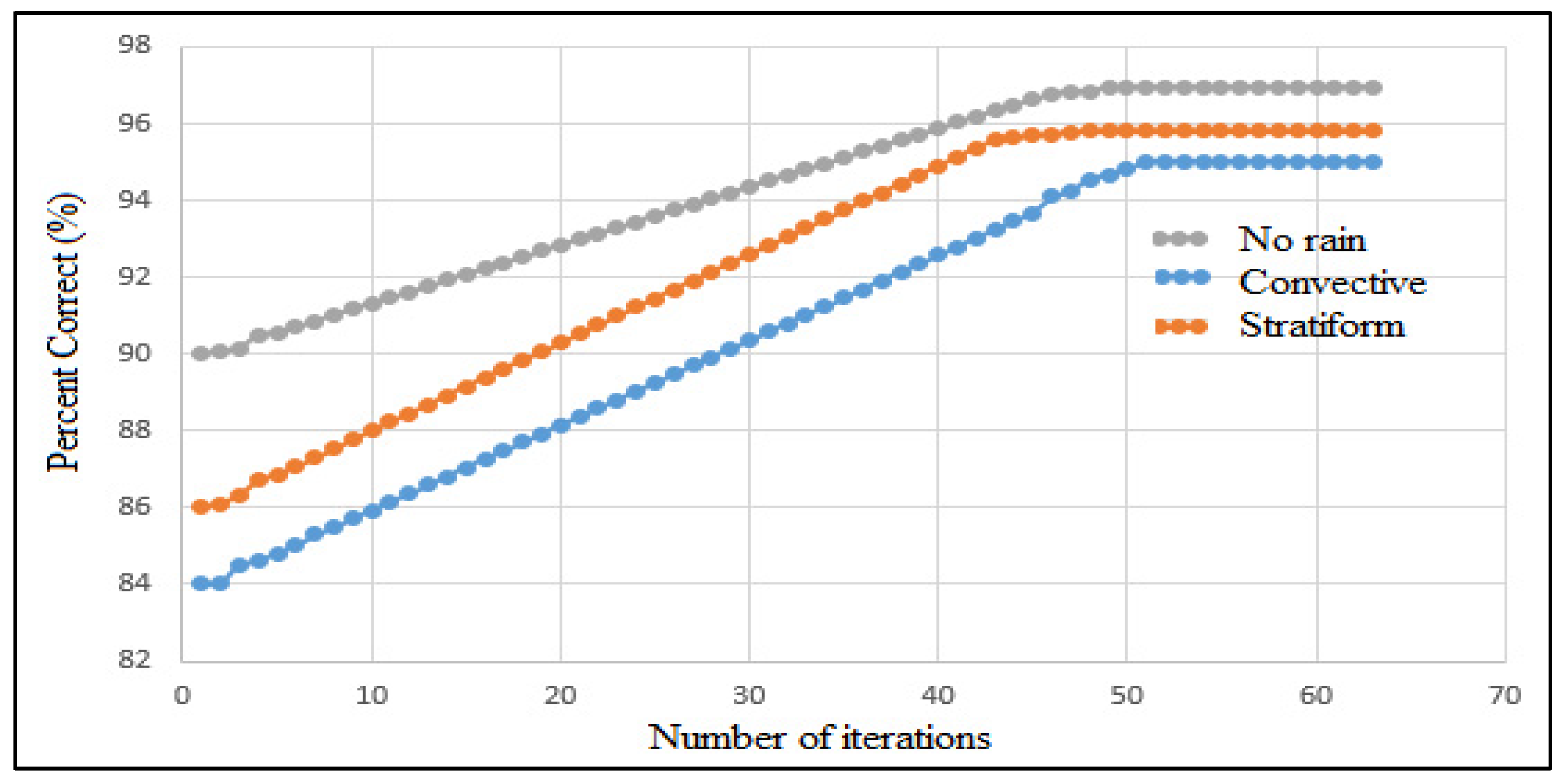
First, we plotted the curve showing the PC parameter as a function of the number of iterations carried out (see Figure 6).

As we can see from the curve as shown in Figure 6, at iteration 50, the results do not change. For this purpose, in what follows, all the results are obtained for iteration 50.

The classification statistical results calculated for the performance evaluation of the SVM, S3VM, and S3VM-FFA models are presented in Table 4 and Table 5 for the three classes.

Table 8. Statistical results of comparison between the SVM model and the S3VM model.

Class	Model	POD (%)	POFD (%)	FAR (%)	Bias	CSI (%)	PC (%)
Convective	S3VM	91	11	30	0.94	73	95
	SVM	78	23	42	0.76	62	84
Stratiform	S3VM	93	09	29	0.96	75	96
	SVM	79	22	41	0.78	64	86
No Convective	S3VM	96	04	23	1.03	78	97
	SVM	81	15	35	1.11	71	90
	Optimal value	100	0	0	1	100	100

shows the first improvement contributed by the S3VM compared to the standard SVM. In

Table 9. Statistical results of comparison between the S3VM model and the S3VM-FFA model.

Class	Model	POD (%)	POFD (%)	FAR (%)	Bias	CSI (%)	PC (%)
Convective	S3VM-FFA	93	9	28	0.97	75	96
	S3VM	91	11	30	0.94	73	95
Stratiform	S3VM-FFA	94	8	27	0.98	76	97
	S3VM	93	9	29	0.96	75	96
No Convective	S3VM-FFA	97	3	21	1.02	80	98
	S3VM	96	4	23	1.03	78	97
	Optimal value	100	0	0	1	100	100

, we observe the second improvement thanks to the S3VM-FFA model.

These statistical results clearly indicate that the S3VM model significantly improved classifications compared to using the standard SVM model. In the case of the convective class, the S3VM model gives a POD, a POFD, and a FAR of 91%, 11%, and 30% against 78%, 23%, and 42% for the SVM model, respectively. The bias is 0.94 for the S3VM model compared to 0.76 for the SVM model. In terms of CSI and PC, the S3VM model always shows the best values. Indeed, the CSI and PC are 73% and 95% for the S3VM compared to 62% and 84% for the SVM, respectively. As we can see, the same trend is observed for both the stratiform class and the non-precipitating class. The difference in values between the S3VM and the SVM is significant. For example, in the stratiform class, the S3VM shows an improvement of up to 14% and 13% for the convective class. For the non-precipitating class, the improvement in results reached 15%.

Although the S3VM model already shows a clear improvement over the standard SVM, the integration of the FFA (S3VM-FFA) further optimizes the performance. As the results show (see Table 8 and Figure 7), S3VM-FFA outperforms the two previous models, particularly for the most difficult classes to discriminate (convective and stratiform). For example, for the convective class, S3VM-FFA achieves a POD of 94% (a 3% increase over S3VM) and an FAR of 25% (a 5% decrease over S3VM), while maintaining a bias close to equilibrium (1.02). In the case of the stratiform class, the POD and FAR are 94% and 27%, respectively, with the S3VM-FFA model, compared to 93% and 29% with the S3VM model.

With regard to the CSI and PC for the convective class, the S3VM-FFA model also shows higher values. Indeed, the CSI and PC are 75% and 96%, respectively, for the S3VM-FFA, compared to 73% and 95% for the S3VM. For the stratiform class, the CSI and PC are 76% and 97%, respectively, for the S3VM-FFA, compared to 75% and 96% for the S3VM.

While the quantitative improvements may appear limited at first glance, the consistent enhancement across all metrics (increase in CSI and PC, reduction in FAR) demonstrates S3VM-FFA’s ability to refine classification accuracy, particularly for ambiguous meteorological cases. This comprehensive improvement, though measured, confirms the approach’s robustness for applications requiring fine discrimination between precipitation classes.

Given its easily identifiable nature, the classification of the non-precipitating class presents the best results compared to the stratiform and convective classes. This characteristic is obtained for the three models S3VM-FFA, S3VM, and SVM. Between the stratiform class and the convective class, we noted a slight difference in terms of superiority for the stratiform class.

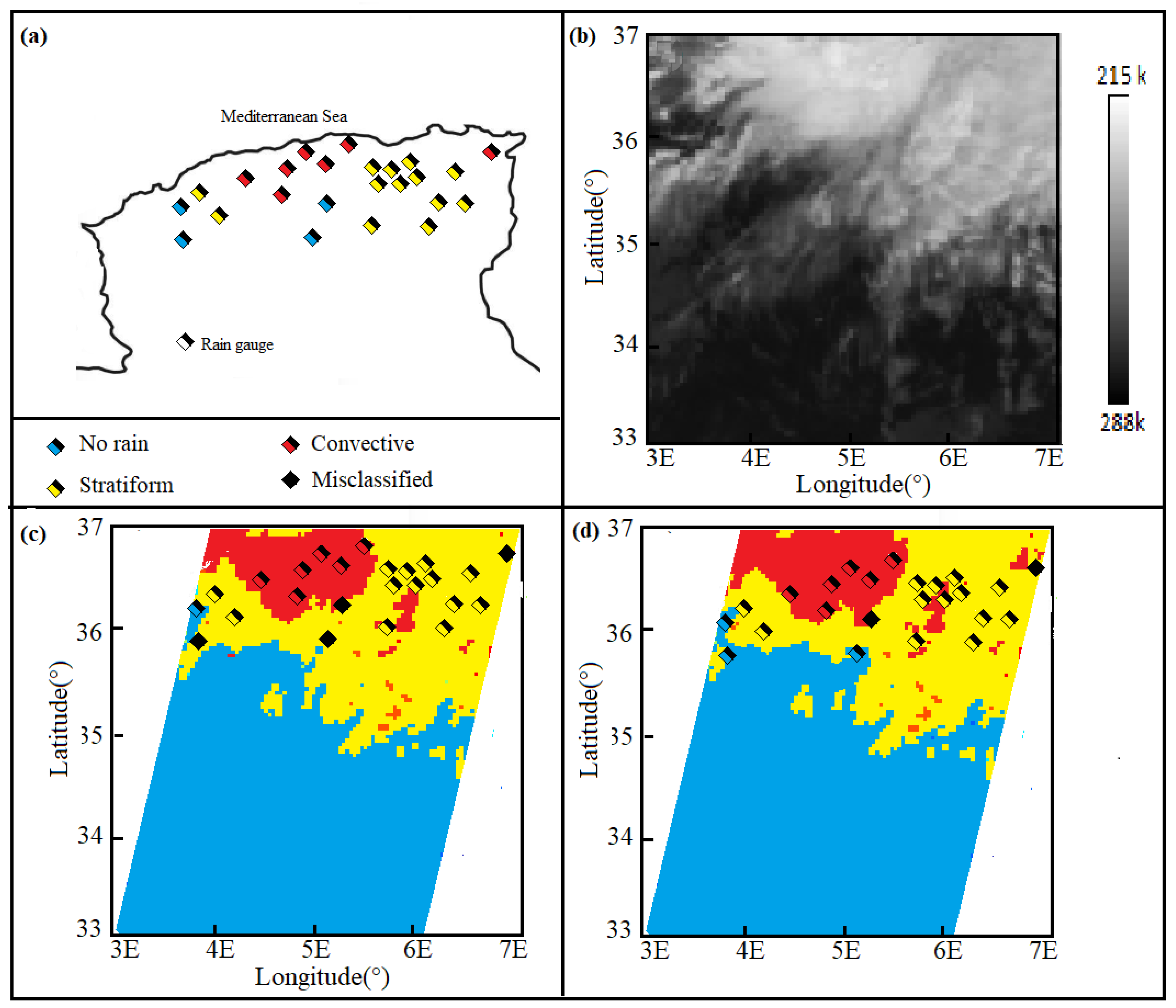
As an illustration, we have classified an instantaneous scene taken by the MSG. The classification results are given by Figure 7. We applied the S3VM-FFA and SVM models for visual comparison.

As shown in Figure 7, this instantaneous scene was completely classified by the three models. However, out of the 24 labeled pixels, with the S3VM-FFA model, we managed to correctly classify 22 pixels compared to 20 pixels for S3VM and 18 pixels for SVM.

5. Precipitation Estimation

The classification results obtained in the previous section are used for precipitation estimation. To do this, we determined a precipitation rate for each class. The non-precipitating class corresponds to a rate of 0 mm h⁻¹. In the case of stratiform and convective classes, we calculated the corresponding precipitation rates using Equations (7) and (8), respectively.

$${RR}_{con}={\displaystyle \frac{\sum _{i=1}^n{Rc}_i}{n}}$$

(7)

$${RR}_{str}={\displaystyle \frac{\sum _{i=1}^k{Rs}_i}{k}}$$

(8)

• RR_con: Mean precipitation rate assigned to the convective class (mm h⁻¹);
• RR_str: Mean precipitation rate assigned to the stratiform class (mm h⁻¹);
• Rc_i: Convective precipitation measurement recorded by rain gauge i during the training period;
• Rs_i: Stratiform precipitation measurement recorded by rain gauge i during the training period;
• n: Total number of measurements identified as convective during the training period;
• k: Total number of measurements identified as stratiform during the training period.

This is the average of the n measurements (resp. k measurements) carried out by the different rain gauges during the learning period for the convective class (resp. stratiform class).

The estimates are determined by applying the S3VM and the hybrid S3VM-FFA models. In order to highlight the contribution of semi-supervised machine learning as the first improvement and the integration of FFA as the second improvement compared to the already known models, we also present precipitation estimation results using a set of techniques based on supervised machine learning. The conditions for implementing these techniques are different from the S3VM-FFA model. Indeed, the techniques are trained using only labeled data represented by MSG data/radar data pairs. These techniques are the following:

The technique combining a support vector machine, artificial neural network, and random forest (SAR), designed for the classification of convective and stratiform rain [14].

The Convective/Stratiform Rain Area Delineation Technique (CS-RADT) developed by [43], separating between convective precipitation and stratiform precipitation using a set of thresholds. The data used were provided from the MSG satellite.

The RF (random forest) technique [36], allowing us to classify rainfall into three classes (no-rain, convective, and stratiform) using random forest theory.

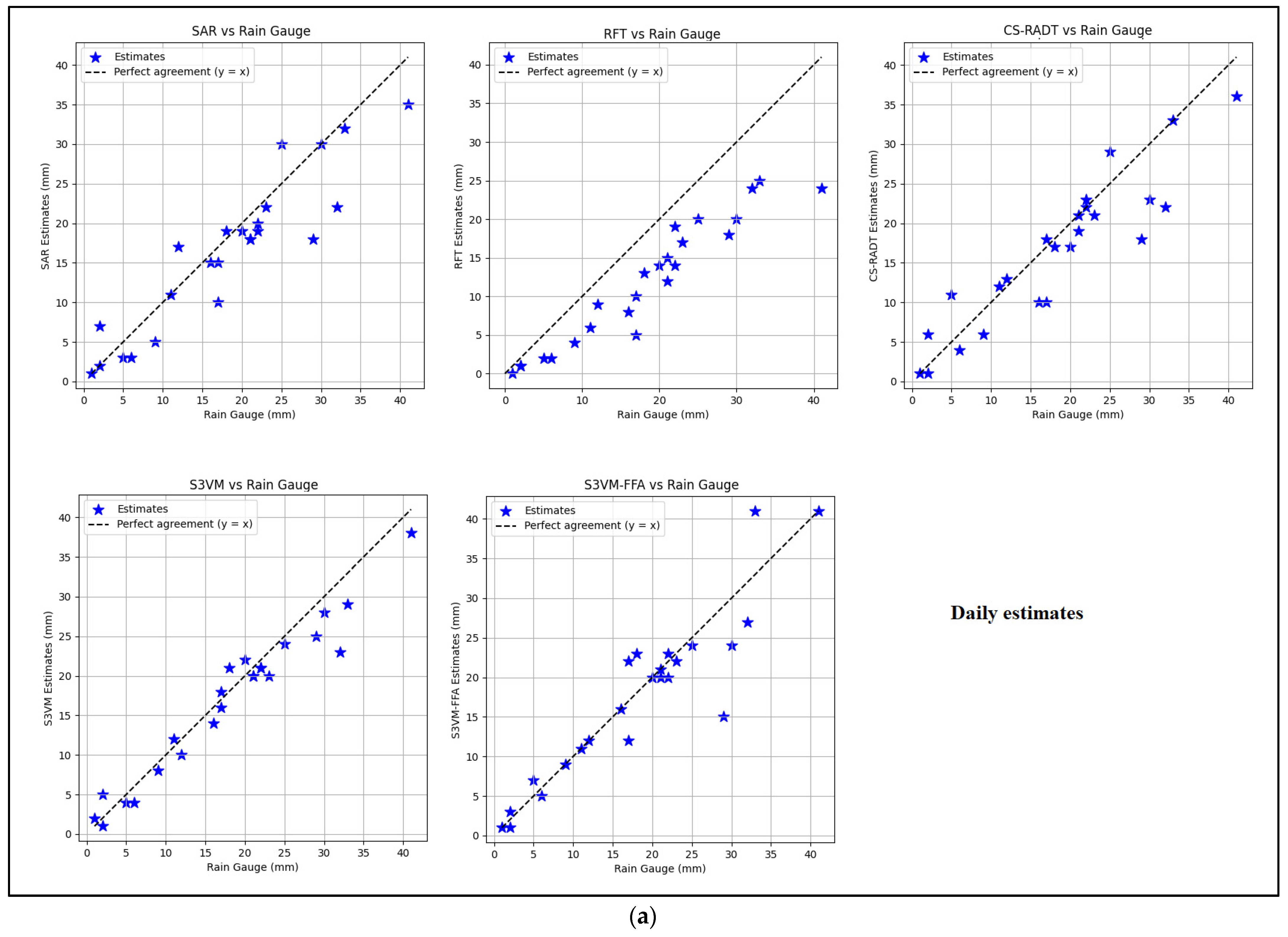
All these techniques operate in two stages: a classification stage and an estimation stage. As with the S3VM-FFA model, the techniques classify precipitation intensities into three classes: the convective class, stratiform class, and non-precipitating class. Precipitation rates are assigned to different classes. Thus, we were able to determine the precipitation accumulations using the occurrences of the classes. The results of the precipitation estimates are shown in Figure 8.

To evaluate method performance, we calculated the bias, RMSD (the root mean square difference), and correlation coefficient. These statistical parameters were derived using standard equations.

$$\mathrm{Bias}={\displaystyle \frac{1}{\mathrm{N}}}\sum _{\mathrm{i}=1}^{\mathrm{N}}\left(E_i-V_i\right)$$

(9)

$$\mathrm{R}\mathrm{M}\mathrm{S}\mathrm{D}=\sqrt{{\displaystyle \frac{1}{\mathrm{N}}}\sum _{\mathrm{i}=1}^{\mathrm{N}}{\left(E_i-V_i\right)}^2}$$

(10)

$$CC={\displaystyle \frac{\sum \left[\left(E_i-\overline{E}\right) \ast \left(V_i-\overline{V}\right)\right]}{\sqrt{\sum {\left(E_i-\overline{E}\right)}^2 \ast {\sum \left(V_i-\overline{V}\right)}^2}}}$$

(11)

where $E_i$ is the estimation corresponding to the rain gauge i, and $V_i$ is the measurement performed by rain gauge i. The statistical results are given in

Table 10. Statistical results for evaluation of techniques.

Method	Bias (mm)	RMSD (mm)	CC (%)
S3VM-FFA	−3	38	96
S3VM	6	43	94
CS-RADT	26	57	84
RF	−18	49	88
SAR	5	46	93

for the entire rainy season for validation data.

In evaluating the S3VM model, we observe a significant improvement in estimates relative to the SVM model. The results correlate strongly with rain gauge measurements of cumulative precipitation, achieving a correlation coefficient of 94% for S3VM compared to 81% for SVM.

The bias indicates a slight overestimation in the S3VM model, whereas the SVM model shows a more pronounced overestimation. Additionally, the root mean square difference (RMSD) indicates that the S3VM model performs better than the SVM model.

The inter-comparison indicates that S3VM surpasses other machine learning and thresholding methods. Notably, S3VM has a correlation coefficient (CC) of 94%, while the CS-RADT, RF, and SAR methods have CCs of 84%, 88%, and 93%, respectively.

When assessing bias, S3VM shows a 6 mm overestimation, which is more balanced than CS-RADT’s 26 mm overestimation, SAR’s 5 mm overestimation, and RF’s 18 mm underestimation.

In terms of the RMSD, S3VM’s value is 43 mm, compared to 57 mm for CS-RADT, 49 mm for RF, and 46 mm for SAR. These results highlight the efficacy of S3VM over the evaluated techniques.

Unlabeled data contain valuable information that has significantly improved our classification and estimation results. The S3VM model has even outperformed supervised machine learning models that utilize a fairly complete dataset. Nevertheless, the large amount of unlabeled data in databases remains untapped by supervised learning techniques.

The S3VM-FFA model shows an exceptional performance in estimating precipitation, surpassing all comparison methods. It has a standardized correlation coefficient of 96% and a mean squared error reduced to 38 mm, which is significantly better than the CS-RADT model (94%, 43 mm) and the SAR model (93%, 43 mm).

With a remarkably low bias of −3 mm, the model suggests a slight systematic underestimation of precipitation. However, this minimal bias is far better than the substantial overestimation of the reference S3VM (60 mm) and is even more precise than SAR (5 mm).

This overall enhancement stems from the dynamic adjustment of hyperparameters and the smart selection of pseudo-labels through the Firefly Algorithm (FFA), which effectively exploits the information inherent in unlabeled data. In contrast to supervised methods like SAR, which require completely labeled datasets, S3VM-FFA achieves a high operational accuracy while utilizing unlabeled data. These findings indicate that S3VM-FFA is a robust and highly accurate method for precipitation estimation.

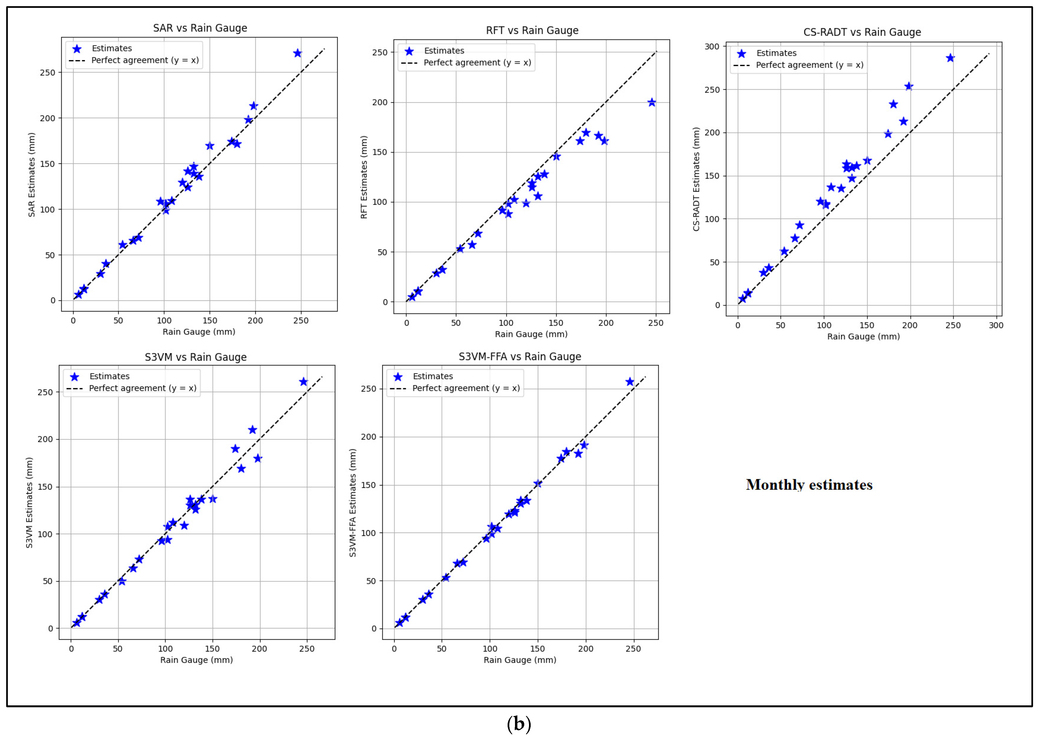
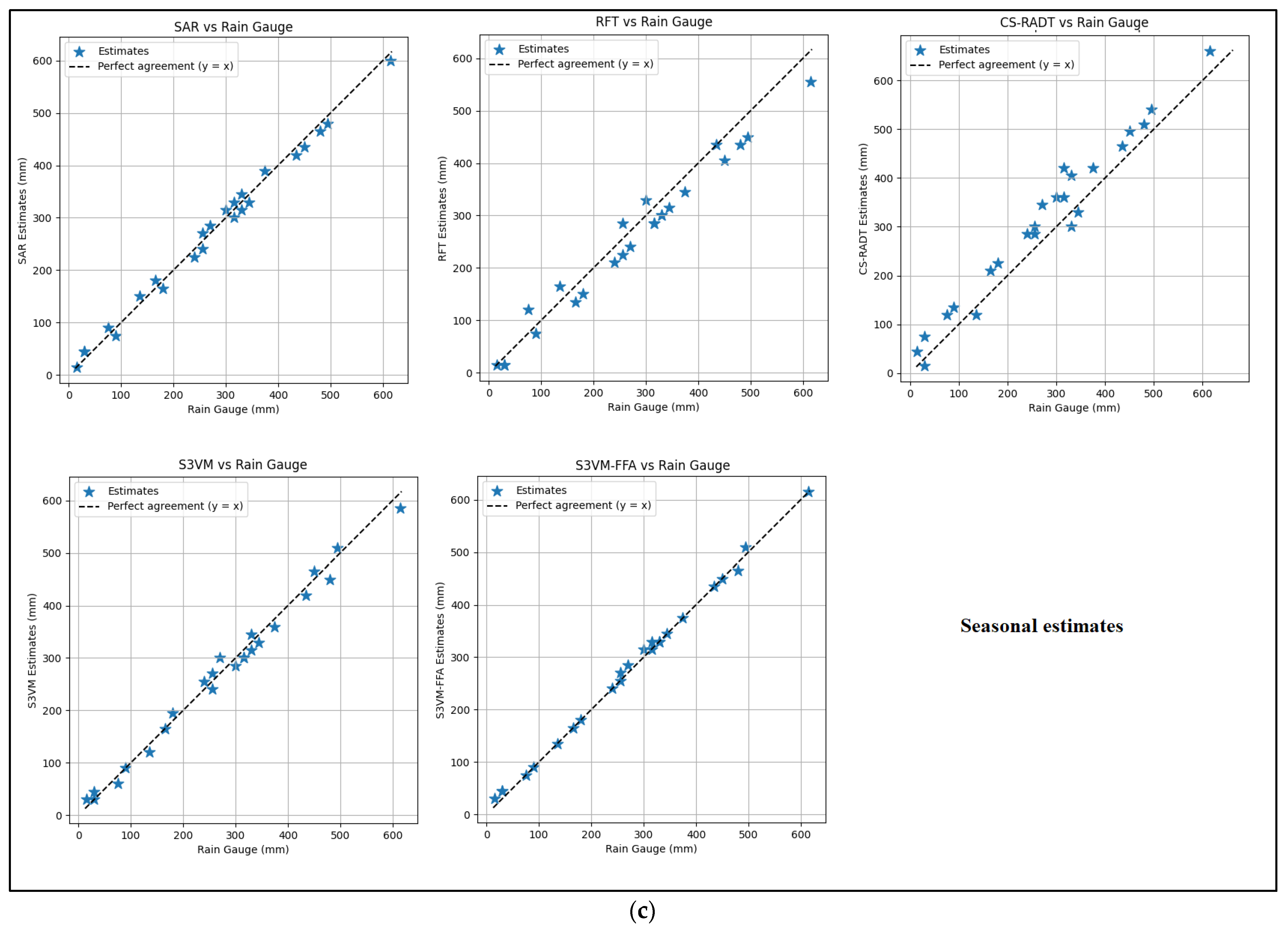
The exploration of daily, monthly, and seasonal estimates (Figure 8) further illuminates the potential seasonal dependence of model performance. At the daily level, the S3VM-FFA model more accurately captures the variability of convective events than the other methods, indicated by its tighter clustering around the perfect agreement line.

On a monthly scale, all models show a reduced dispersion, but S3VM-FFA maintains a higher correlation and lower bias, suggesting its robustness in aggregating precipitation over longer periods. Seasonally, the model aligns excellently with rain gauge measurements, showing a stable performance across different precipitation types, whether they are stratiform or convective.

This analysis indicates that the S3VM-FFA model reliably achieves a high accuracy throughout the year. It capitalizes on dynamic hyperparameter adjustments and effectively leverages unlabeled data, which together enhance its generalization capabilities across seasonal differences in precipitation types.

6. Conclusions

We classified remote sensing data obtained from the MSG satellite and produced precipitation estimates using the S3VM model, which employs semi-supervised machine learning. This model enabled the segmentation of precipitation intensities into three distinct classes: convective, stratiform, and non-precipitating. The primary contribution of this research involves leveraging both unlabeled and labeled data. While labeled data were infrequent, they provided essential initial training for the model. The abundant unlabeled data, filled with rich and varied information, allowed us to refine the model’s learning capabilities.

For the first improvement, we applied the S3VM model to classify pixels within MSG images. To evaluate the model’s performance, we calculated several statistical evaluation parameters. Subsequently, for the second enhancement, we hybridized the S3VM model with the Firefly metaheuristic (S3VM-FFA) to find the optimal hyperparameters (C, γ, and C*) and thereby enhance both classification and precipitation estimation results.

In this study, the standard SVM model trained on labeled data was also applied for comparison purposes. The results indicate that the S3VM model outperforms the standard SVM. Statistical parameters revealed that the S3VM model improved classification results by up to 14% compared to the SVM model, while the S3VM-FFA model enhanced results by 17% compared to SVM.

This trend was consistent across all three classes. However, the identification of the non-precipitating class showed a stronger correlation with rain gauge data for both models.

From the classification results, we also made precipitation estimates. For each class, we assigned a precipitation rate based on pluviographic data. The cumulative precipitation rate was calculated based on the occurrence of each class during the specified period.

The findings showed that S3VM estimates correlate significantly with pluviographic measurements when compared to those from the SVM model. The correlation coefficient for the S3VM model is 0.94, compared to 0.81 for the SVM model.

The unlabeled data greatly enhanced the model’s learning adjustment. By utilizing the S3VM-FFA hybrid model, we achieved an even higher correlation of 0.96, attributed to the optimization of S3VM hyperparameters by the Firefly Algorithm.

We carried out a cross-comparison to highlight the potential of the semi-supervised machine learning concept, especially in relation to supervised learning models and thresholding methods. Alongside the S3VM-FFA (Semi-Supervised Support Vector Machine optimized by the Firefly Algorithm), we deployed S3VM and SVM models, as well as three additional rainfall estimation techniques: RF, SAR, and CS-RADT.

The results confirmed the superiority of semi-supervised approaches, particularly with the S3VM-FFA model, which merges the advantages of classic S3VM with metaheuristic optimization for improved accuracy and robustness.

The statistical evaluation parameters demonstrated that the S3VM-FFA method offers a better correlation than the other techniques, including the standard S3VM. While the S3VM model displayed a slight overestimation, the S3VM-FFA resulted in an even lower bias, attesting to the effectiveness of optimization via FFA.

These findings can be explained by the semi-supervised methods’ ability to leverage both labeled and unlabeled data, enriching their insights beyond what is captured by supervised approaches. Purely supervised models may face errors due to imperfect data labeling, while S3VM-FFA utilizes all available data for a more comprehensive and reliable learning process.

Initial learning is guided by labeled data, while unlabeled data, combined using the semi-supervised method and optimized by the FFA, strengthens the model’s generalization.

Future research may focus on incorporating complementary satellite datasets like Sentinel or GPM and examining advanced deep semi-supervised architectures to better characterize precipitation both spatially and temporally.