A Regional Aerosol Model for the Middle Urals Based on CALIPSO Measurements

Abstract

The present work aims to develop a regional Middle Urals Aerosol model (MUrA model) based on the joint analysis of long-term ground-based photometric measurements of the Aerosol Robotic NETwork (AERONET) and the results of lidar measurements of the CALIPSO (Cloud-Aerosol Lidar and Infrared Pathfinder Satellite Observation) satellite relying on information on the air trajectories at different altitudes calculated using the HYSPLIT (Hybrid Single Particle Lagrangian Integrated Trajectory model) software package. The MUrA model contains parameters of normalized volume size distributions (NVSDs) characterizing the tropospheric aerosol subtypes detected by the CALIPSO satellite. When comparing the MUrA model with the global CALIPSO Aerosol Model (CAMel), we found significant differences in NVSDs for elevated smoke and clean continental aerosol types. NVSDs for dust and polluted continental/smoke aerosol types in the global and regional models differ much less. The total volumes of aerosol particles along the atmospheric column reconstructed from satellite measurements of the attenuation coefficient at a wavelength of 532 nm based on the regional MUrA model and global CAMel are compared with the AERONET inversion data. The mean bias error for the regional model is 0.016 μm³/μm², and 0.043 μm³/μm² for the global model.

1. Introduction

Atmospheric aerosols have a multifaceted impact on the radiation balance of the Earth, thus affecting the climate. They interact with short-wave solar and infrared radiation of the Earth’s surface [1,2,3]; participate in cloud formation and processes happening inside clouds [4,5]; can change the reflective properties of the underlying surface [6,7]. Further, a high content of solid particles in the air can cause serious consequences for human health, including cardiovascular and respiratory diseases [8,9,10,11]. The key parameters in modeling the influence of aerosol particles on atmospheric processes are their qualitative (aerosol composition and its microphysical parameters) and quantitative characteristics.

Without any extended direct aerosol monitoring networks, one of the ways to obtain information about the aerosol content in the atmosphere is to build regression models linking direct ground-based measurements of aerosol concentration at one or more monitoring points, integral characteristics of remote sensing of the atmosphere (aerosol optical depth) and meteorological parameters [12,13,14]. With this approach, it is possible to estimate the spatial distribution of surface aerosol concentrations based on remote satellite sensing of the atmosphere in the studied region [15,16,17]. Another approach to estimating aerosol spatial distribution is to use methods relying on the information about the atmosphere dynamics [18,19]. However, these approaches fail to estimate the vertical distribution of aerosol in the atmosphere.

The vertical distribution of aerosol can be obtained as a result of direct measurements aboard aircrafts [20,21] or unmanned aerial vehicles [22,23] at different altitudes.

Lidar measurements are one of the most promising methods to determine the vertical profile of aerosol, because they enable restoring the microphysical parameters of aerosol, solving the inverse problem [24,25,26,27]. To successfully solve the inverse problem, lidar needs to be working at least at three wavelengths. More often, to restore the vertical structure of the microphysical parameters of aerosol, lidar measurements are to be taken together with other measurements, such as direct parallel ground-based [28] or aircraft [29,30] measurements of aerosol concentrations. Lidar measurements are also often supplemented by photometric measurements [25,31,32,33]. Such ground-based and/or aircraft measurements are usually taken as part of planned scientific campaigns (expeditions); they require careful preparation and are limited in space and/or time. Such a problem of spatial and temporal limitation of data is currently solved by continuous satellite remote sensing of the Earth’s atmosphere [34].

Nowadays, global lidar measurements are provided by the CALIPSO (Cloud-Aerosol Lidar and Infrared Pathfinder Observation) satellite equipped with Cloud-Aerosol Lidar with Orthogonal Polarization (CALIOP) operating at two wavelengths of 532 and 1064 nm [35]. The CALIPSO lidar Level 2 aerosol profile data offer a big number of products, including the vertical distribution of backscatter, extinction and depolarization coefficients. Apart from that, CALIPSO provides information on the types of atmospheric objects (clean air, clouds, tropospheric and stratospheric aerosol, etc.) as well as on tropospheric aerosol subtypes. The algorithm of the fourth version of CALIPSO classifies tropospheric aerosol based on the data of the backscatter coefficient, the depolarization coefficient, the type of underlying surface, and the altitude of the studied aerosol layer. Thus, it identifies seven subtypes: pure marine, dust, polluted continental/smoke, pure continental, polluted dust, elevated smoke, and dusty marine [36]. The microphysical and some optical parameters of the listed subtypes of tropospheric aerosol make up the CALIPSO Aerosol Model (CAMel) [37,38]. This is a global model often used to reconstruct aerosol concentrations from the CALIPSO satellite data, although it does not take into account regional peculiarities of atmospheric aerosol properties [39,40].

The purpose of the work is the development of a regional aerosol model for the Middle Urals which determines the microphysical parameters of the tropospheric aerosol subtypes provided by CALIPSO. The new regional model will allow more accurate reconstruction of aerosol concentrations vertical profiles based on satellite lidar measurements. This paper is organized as follows. Section 2 presents the initial data, including the results of AERONET (Aerosol Robotic NETwork) photometric measurements in the Middle Urals, air flow trajectories calculated by the HYSPLIT (Hybrid Single Particle Lagrangian Integrated Trajectory model) software package, and CALIPSO lidar measurements. Also, this section describes the algorithm of the combination of CALIPSO vertical profiles with AERONET data on the atmospheric column aerosol content. Then, the authors offer their regional aerosol model for the Middle Urals and present the results of reconstructing the vertical profiles of atmospheric aerosol volume concentrations calculated based on the methodology from [40] (Section 3). At the end of Section 3, the data obtained are compared with the aerosol particles volumes along the atmospheric column from the AERONET inversion algorithm.

2. Materials and Methods

2.1. AERONET Photometric Measurements

In the present work, we used the volume particle size distributions reconstructed from photometric measurements taken since 2007 till 2021 at the AERONET site [41] located in the Middle Urals (Yekaterinburg, (57.038 N, 59.545 E)). The research is based on the Level 2 data, which are the most reliable error-filtered data. The analysis includes a total of 1091 measurements.

The standard products of AERONET inversion are the volume of aerosol particles along the atmospheric column, the median radius, and the standard deviation from the median radius for two aerosol fractions, which help approximate the real aerosol particle size distribution in the form of a bimodal lognormal distribution [42]. The works focusing on the typification of atmospheric aerosols present the volume particle size distribution as follows:

$$\frac{\mathrm{d}V\left(r\right)}{\mathrm{d} \mathrm{l}\mathrm{n} r}=V_t\sum _{i=1}^2\frac{v_i}{\sqrt{2\pi }{\sigma }_i}exp\left(\frac{-{(\ln r-\ln {\mu }_i)}^2}{2{\left({\sigma }_i\right)}^2}\right)=V_t{\left(\frac{\mathrm{d}V\left(r\right)}{\mathrm{d} \mathrm{l}\mathrm{n} r}\right)}_{norm}$$

(1)

where i is the index denoting the mode of aerosol particle size distribution: 1 corresponds to the fine aerosol fraction, 2 to the coarse aerosol fraction; $V_t=\sum _{i=1}^2{V}_i$ is the total volume of aerosol particles along the atmospheric column (µm³/µm²); $V_i$ is the volume of the i^th mode along the atmospheric column; $v_i=\frac{V_i}{V_t}$ is the aerosol volume fraction of the i^th mode; r is the radius of aerosol particles; ${\mu }_i$ is the volume median radius of the i^th mode; ${\sigma }_i$ is the standard deviation from the volume median radius for the i^th mode; ${\left(\frac{\mathrm{d}V\left(r\right)}{\mathrm{d} \mathrm{l}\mathrm{n} r}\right)}_{norm}$ is the normalized volume size distribution (NVSD) of aerosol particles, i.e., the integral of this function over the entire range of radii is equal to 1. It is believed that, under idealized conditions, the total aerosol volume along the atmospheric column is an extensive parameter and depends on the degree of aerosol concentration in the atmosphere, while the normalized size distribution is determined by intensive parameters and depends on what type of aerosol is present in the atmosphere.

It is worth noting that the results of the AERONET inversion essentially provide information on aerosol in atmospheric conditions, taking into account the humidity of the environment, i.e., reproduce the size distribution function of moistened aerosol particles.

The AERONET measurements in the Middle Urals were mainly taken in the warm season—from April to October—due to the climate of the region (few sunny days in winter) and the need for calibration procedures, for which the photometer was returned to NASA GSFC (National Aeronautics and Space Administration, Goddard Space Flight Center) every winter for intercomparison with reference instruments [43].

2.2. Air Trajectories Modelling

The HYSPLIT software package (Hybrid Single Particle Lagrangian Integrated Trajectory model) [44] enables to restore forward and backward trajectories of elementary air parcels (hereinafter air trajectories). Three-dimensional fields of meteorological data of the Northern Hemisphere obtained from the National Center for Environmental Prediction (NCEP) Global Data Assimilation System (GDAS1) [45] were used as input information to calculate the air trajectories. The spatial resolution of the initial meteorological information was 1° × 1° with 23 pressure levels by altitude, while the time resolution was three hours.

The starting position of the trajectories corresponds to the coordinates of the AERONET site in the Middle Urals. The starting moments of the air trajectories correspond to the moments of photometric measurements. The air trajectories duration was 12 h with the interval of one minute, while the starting heights of the air trajectories were from 250 m to 9750 m above the ground level with the interval of 500 m (20 levels in total).

Based on numerous back trajectories at the altitude of 250 m, we determined a 12-h zone of influence on the measuring device—such an area where any event related to atmospheric pollution could potentially be recorded at the device location. As a result, the analyzed area was (54°–65°) E and (54°–61°) N.

2.3. CALIPSO Satellite Data

CALIPSO is an American and French research satellite in a sun-synchronous polar orbit launched on 28 April 2006. The main task of CALIPSO is to study the three-dimensional structure of clouds and atmospheric aerosol layers. CALIPSO, inter alia, is equipped with CALIOP [46].

To compare satellite data on aerosol types with microphysical characteristics obtained from ground-based photometric measurements, we relied on the CALIPSO satellite data from 2007 to 2021, which fell into the 12-h influence zone of the AERONET site in the Middle Urals, and used information on vertical distributions of atmospheric object types (vertical feature mask) and tropospheric aerosol types.

The CALIPSO automated aerosol classification algorithm based on the measurement of backscatter and depolarization coefficients, the type of underlying surface, and the height of the aerosol layer is described in detail in [36]. The CALIPSO version 4.20 Level 2 aerosol profile algorithm classifies the measured signal into seven types of objects: 1. clean air; 2. clouds; 3. tropospheric aerosol; 4. stratospheric aerosol; 5. the Earth’s surface; 6. areas below the ground level; 7. lack of a signal (total absorption). There are also seven subtypes for the type of “tropospheric aerosol”: 1. clean marine (CM); 2. dust (DU); 3. polluted continental/smoke (PC/SM); 4. clean continental (CC); 5. polluted dust (PD); 6. elevated smoke (ES); 7. dusty marine (DM).

To increase the reliability of the initial data, it is necessary to use additional filtering and quality flags that are provided in each source file. The values of the extinction coefficient should be in the range from 0 to 1.25 km⁻¹. The integral attenuated backscatter should be ≤0.01 sr⁻¹. The Cloud-Aerosol Discrimination Score (CAD_Score) parameter ensures the reliability of the classification of the measured particles as aerosol (from −100 to 0) or a cloud (from 0 to 100). Therefore, if the value is −100, the particle is recognized as aerosol with 100% reliability. In the current work, we have used the range of −100 ≤ CAD_Score ≤ −20. The Extinction Quality Check flag (Extinction_QC_Flag_532) parameter proves the correctness and a possibility of solving the problem to restore the extinction coefficient at the wavelength of 532 nm using the lidar ratio for different types of aerosols. The values of this flag must take one of the following values: 0, 1, 2, 16 or 18 [47].

2.4. Methodology of the Combination of AERONET with CALIPSO Data

In this paper, we propose an approach where the microphysical characteristics along the atmospheric column restored by the AERONET inversion algorithm are correlated with various types of the CALIPSO classification atmospheric objects, taking into account the heights at which they are detected. To this end, we search for intersections of forward and backward air trajectories starting at different heights from the AERONET site location at the measurements moments with the CALIPSO satellite tracks. Thus, a set of data is formed, which serves as the foundation for the regional model of the microphysical characteristics of atmospheric aerosol in the Middle Urals.

To reduce the amount of initial information, satellite data were averaged. For example, Figure 1a shows a part of the CALIPSO satellite track on 25 August 2017, which fell into the analyzed area and passed in close proximity to the monitoring station. The analyzed area is marked by the red frame. The blue frame shows the space scanned by the CALIPSO satellite. The AERONET site located in the Middle Urals is marked with a red asterisk. Also, you can see the administrative boundaries of the regions plotted on the map for convenience. The satellite was less than two minutes above the studied area, and during this time it passed a distance equal to the track of approximately 600 km long on the Earth’s surface. Initially, this dataset contains 64,239 records (161 points horizontally and 399 levels vertically). Since the object of this study is tropospheric aerosol, satellite data at heights above the troposphere (altitudes > 12 km above the mean sea level) are discarded. First, the data are averaged horizontally along the satellite track with the interval of approximately 15 km and then vertically with the interval of approximately 500 m from the Earth’s surface. The final dataset is shown in Figure 1b and contains 820 entries (41 points horizontally and 20 levels vertically). The type of aerosol is determined by ‘voting’, i.e., we had to determine the type of aerosol most often found in the cell within which parameters are averaged. Figure 1 shows only the data on the subtype of tropospheric aerosols. Therefore, light blue areas may correspond to such atmospheric objects as ‘Clean Air’ or ‘Cloud’ types.

For satellite tracks passing at a distance from the AERONET site, we analyzed their intersections with the trajectories of air flows (forward and backward). Figure 2 illustrates a part of the track from Figure 1 and the backward air trajectories intersecting it, starting at different altitudes from the AERONET site at the measurement moment—26 August 2017 06:06:00 UTC (Coordinated Universal Time). The start positions of the trajectories are marked with red dots, the intersection points of the air trajectories and the satellite track are marked with red crosses. In general, air trajectories starting at different heights intersect the satellite track in different points. Under the CALIPSO classification, we determine the type of an atmospheric object or the type of aerosol (hereinafter simply the type of an atmospheric object) at the intersection points. If several intersections of the air trajectories and satellite tracks are fixed at the same moment of the AERONET measurement, such a value of the type of an atmospheric object is selected that has the minimal difference between the time of the satellite’s flight and the time when the air flow trajectory reaches the intersection point. In this way, we receive a table containing data on the NVSD parameters restored by AERONET, characterizing the aerosol content along the entire atmospheric column and data on the type of atmospheric objects by the CALIPSO classification at different altitudes compared with them.

In Figure 3 is shown the statistical characteristics of the total aerosol volume along the atmospheric column (a) and fine aerosol volume fraction (b) at the AERONET site, depending on the height and type of aerosol by the CALIPSO data. The figure shall be interpreted as follows. If a specific type of aerosol was detected at a certain height, volume concentrations (Figure 3a) or fine aerosol volume fractions (Figure 3b) were reconstructed at the monitoring site with the values reflected in the box plot. In Figure 3 and box plots below, the horizontal line inside the box represents the median, the white dot indicates the arithmetic mean, while the black dots indicate outliers that are beyond the 1.5 interquartile distance. The upper part of the graph above each box indicates the sample size for which the corresponding box was built, i.e., the number of cases when the AERONET measurement could be compared with a specific type of aerosol by the CALIPSO classification.

It can be seen that the most common type of aerosol found in the region of the Middle Urals is PD. The rarest type of aerosol—CC—is not shown in the figure due to the small number of cases where it could be matched to AERONET data and the consequent non-representative box plots. There is also absolutely no statistical data on the CM and DM aerosol types because the analyzed area is located in the depths of the continent. More often, aerosol is found closer to the Earth’s surface, in the lower layer of the atmosphere up to 5 km thick.

If DU is found in the lower layers of the atmosphere at the altitude of up to 3 km, the average total volume concentration along the atmospheric column is approximately 0.1 µm³/µm². There are very few cases of dust aerosol detection in the layer from 3 to 7 km. And above 7 km, the number of cases is approximately 10 for each altitude, but the concentration is obviously less. That is, even if DU is determined at high altitudes, such cases demonstrate low values of the total volume of aerosol particles along the atmospheric column. Probably, such aerosol layers are formed as a result of long-range transport of desert dust. At the same time, Figure 3b shows that coarse fraction prevails at almost all altitudes, while fine fraction is predominantly less than 0.5.

The PC/SM type of aerosol is observed at altitudes of up to 2.5 km (by the CALIPSO classification algorithm, it is determined for aerosol layers whose upper boundary is below 2.5 km). The moments of detection of this aerosol type demonstrate the values of aerosol volume concentrations of approximately 0.05 µm³/µm², and they vary very slightly with altitude.

The values of total volume concentrations along the atmospheric column compared with the PD type of aerosol vary slightly with altitudes of up to 6 km. A certain number of cases of elevated concentrations (high median) are observed in the layer of 8–9 km. The average values of fine fraction for the PD type of aerosol up to heights of 4.5 km vary slightly with altitude and are approximately 0.5, then they grow to 0.7 at altitudes from 5 to 6 km, and then decrease to approximately 0.3 at the height of 9 km.

If the ES aerosol type is observed, the average volume concentrations of aerosol increase up to 0.15 µm³/µm² at certain altitudes. Average concentrations vary slightly: first, they decrease below 2.5 km, and then increase to the height of 5 km. Above 5.5 km and up to 9 km, there are extremely low values with low dispersion, but there are very few cases when this type of aerosol is determined in this altitude range. High concentrations are observed in the layer of 8–9 km, but due to their insufficient number, it can be assumed that these measurements are episodic events associated with big fires remote from the analyzed area.

For the PC/SM and ES aerosol types, fine aerosol fraction prevails at all altitudes.

3. Results and Discussion

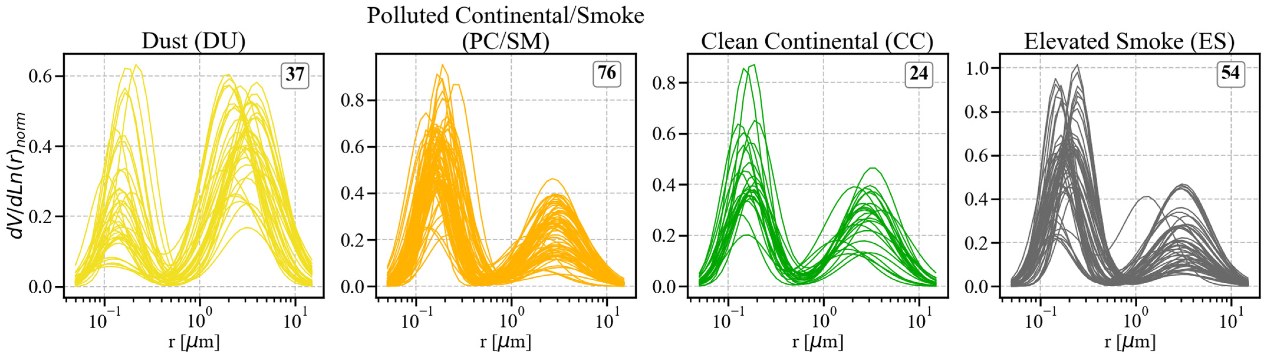
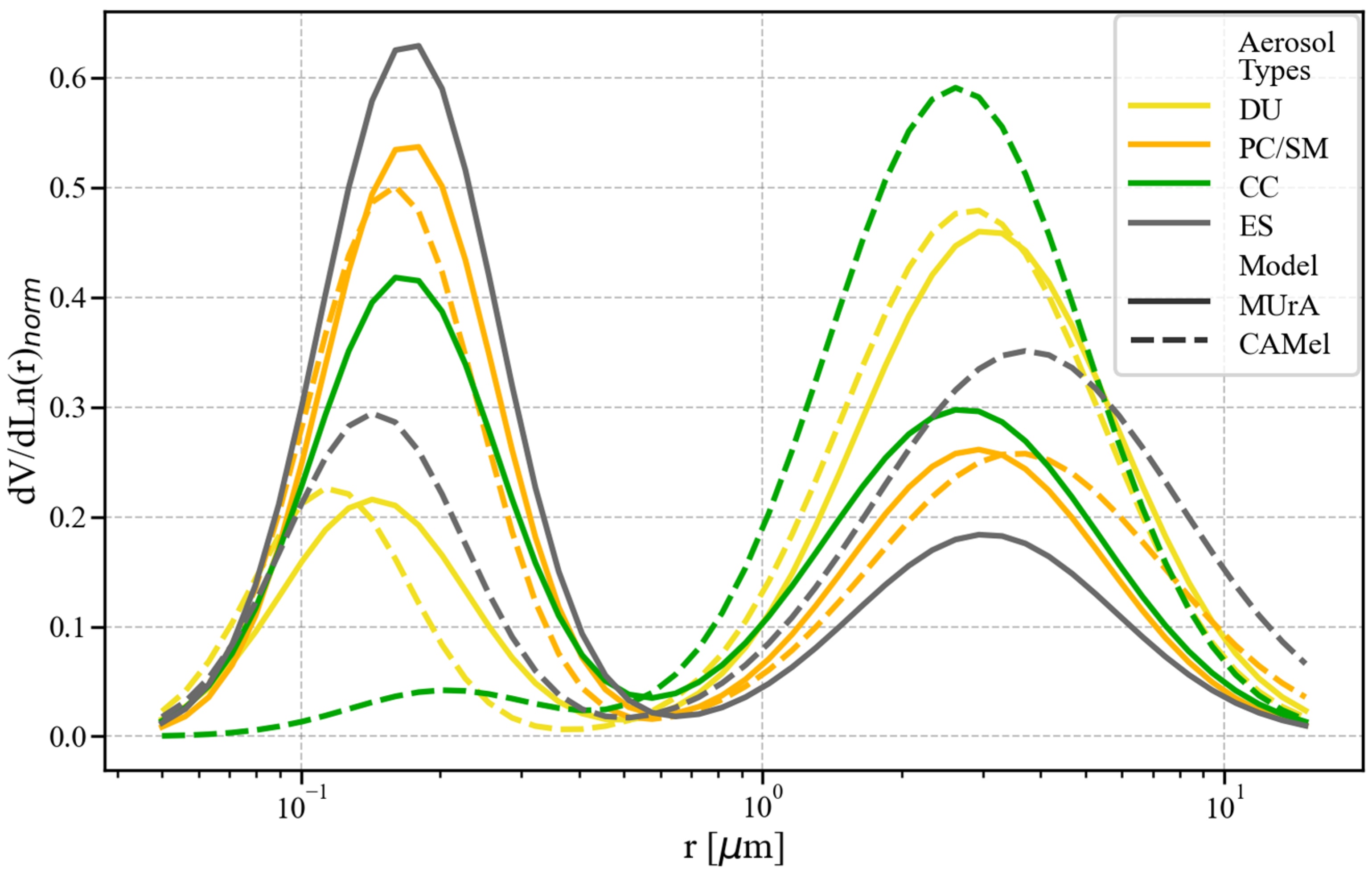
3.1. Aerosol Model for the Middle Urals

Based on the obtained data, we determine the Middle Urals Aerosol model (MUrA model), which contains parameters of NVSDs, characterizing the aerosol types determined by the CALIPSO satellite. Since AERONET determines the characteristics of aerosol along the entire atmospheric column, that is, a mixture of different aerosol types, it is necessary to determine the cases when this mixture is close to uniform.

For this purpose, there is a range of different types of atmospheric objects for each moment of AERONET measurements, depending on the frequency of their occurrence at different altitudes. For the analysis, we select cases when:

-

Clean air and tropospheric aerosol with a specific subtype are the first or second most common types of atmospheric objects;

-

AERONET measurement (along the entire atmospheric column) was able to match a specific type of atmospheric object at least 10 out of 20 altitudes;

-

The total proportion of heights compared with clean air and specific types of tropospheric aerosol is more than 75%.

Figure 4 represents the NVSDs of aerosol particles by the AERONET data, which we were able to relate with a certain aerosol type by the CALIPSO classification in accordance with the above criteria. The largest number of NVSDs proved to be in compliance with the PC/SM (76 measurements) and ES (54 measurements) aerosol types.

Figure 5 demonstrates the statistical characteristics of the parameters of NVSDs of aerosol particles compared with different aerosol types. It can be seen that coarse aerosol fraction prevails for the DU type, while fine fraction obviously prevails for the PC/SM and ES types. The total volume concentrations are noticeably higher for DU and ES aerosol types.

Median values were selected as distribution parameters (volume fraction, median radius, standard deviation from median radius for two aerosol modes) characterizing a specific aerosol type in the developed MUrA model. Moreover, for fine and coarse fractions, we first established their ratio and only then determined the median, on the basis of which the characteristic values of the volume fractions were reconstructed. This procedure equals the sum of final fine and coarse volume fractions to one. The NVSDs parameters of aerosol particles obtained in this way for the DU, PC/SM, CC and ES aerosol types by the CALIPSO classification are shown in

Table 1. Parameters of the normalized volume size distribution of aerosol particles for different aerosol types by the CALIPSO classification in the Middle Urals region.

Aerosol Type	Volume Fraction		Mean Radius		Standard Deviation
	Fine	Coarse	Fine	Coarse	Fine	Coarse
DU	0.25	0.75	0.144	3.079	0.462	0.649
PC/SM	0.579	0.421	0.171	2.917	0.428	0.642
CC	0.488	0.512	0.168	2.722	0.464	0.685
ES	0.696	0.304	0.172	3.038	0.439	0.659

Note: DU—dust, PC/SM—polluted continental/smoke, CC—clean continental, and ES—elevated smoke.

. The model was not meant for the PD aerosol type, as it is a combination of DU with PC/SM or ES aerosol types depending on the height.

Figure 6 shows the NVSDs of aerosol particles for various aerosol types for the Middle Urals by the CALIPSO classification built on Table 1 data. For comparison, you can see the dashed graphs of NVSDs used in the global CAMel [38]. NVSDs differ significantly for the ES and CC aerosol types. For the ES aerosol type, the resulting regional MUrA model has a significantly predominant fine fraction ($v_1$ = 0.696), while in CAMel $v_1$ = 0.329. Also, for the CC aerosol type, fine aerosol fraction in the MUrA model ($v_1$ = 0.488) significantly exceeds the corresponding value in CAMel ($v_1$ = 0.05). Possible reasons for these differences could be the specific aerosol sources, special aspects of the long-range transport, regional environmental and meteorological conditions. NVSDs for DU and PC/SM aerosol types global and regional models differ much less.

3.2. Reconstruction of the Vertical Profiles of the Aerosol Concentration

The developed regional model of aerosol microphysical characteristics can be used to estimate concentrations (volume and number) of aerosol particles based on lidar measurements of the CALIPSO satellite over the Middle Urals. There are various methods for estimating aerosol concentrations based on lidar ground-based [28,32] and satellite measurements [39,40]. We will use the OMCAM (Optical Modeling of CALIPSO Aerosol Microphysics) technique, which is described in detail in the following works [40,48].

Relying on the OMCAM technique, the volume ($C_v$) and number ($C_n$) aerosol concentrations are defined as:

$${\left(C_v\right)}_{i,j}=A_{i,j}\alpha$$

(2)

$${\left(C_n\right)}_{i,j}=B_{i,j}\alpha$$

(3)

where i and j set the size ranges of aerosol particles for which concentrations are calculated; $A_{i,j}$ is the conversion factor to restore the volume concentration of aerosol particles; $B_{i,j}$ is the conversion factor to restore the number concentration of aerosol particles; $\alpha$ is the attenuation coefficient at the wavelength of 532 nm by CALIPSO measurements. Let us note that lidar ratios used in the CALIPSO version 4 aerosol classification algorithm were adjusted compared to the previous versions based on the results of atmospheric measurements [36] and are not necessarily related to the CAMel.

Conversion factors depend on the considered range of particle sizes and on the type of aerosol (a form of NVSD):

$$A_{i,j}=\frac{1}{{\alpha }_{norm}}{\int }_i^j{\left(\frac{\mathrm{d}V\left(r\right)}{\mathrm{d} \mathrm{l}\mathrm{n} r}\right)}_{norm}\mathrm{d}\ln r$$

(4)

$$B_{i,j}=\frac{1}{{\alpha }_{norm}}{\int }_i^j{\left(\frac{\mathrm{d}N\left(r\right)}{\mathrm{d} \mathrm{l}\mathrm{n} r}\right)}_{norm}\mathrm{d}\ln r$$

(5)

where ${\left(\frac{\mathrm{d}V\left(r\right)}{\mathrm{d} \mathrm{l}\mathrm{n} r}\right)}_{norm}$ is number size distribution normalized by particle volume; ${\alpha }_{norm}$ is the attenuation coefficient at the wavelength of 532 nm calculated on the basis of the NVSD of aerosol particles. You can find formulas linking the volume and number size distributions of the aerosol particle, for example, in the following work [49].

For the calculation of ${\alpha }_{norm}$, the modeled optical properties of ensembles of aerosol particles (MOPSMAP) package are used [50]. To calculate the extinction coefficient, it is necessary to set not only the size distribution, but also the integrated refractive index. It is worth noting that the AERONET inversion algorithm, among other parameters, restores the refractive index; however, this parameter reaches low uncertainty only at high aerosol load (the aerosol optical depth at 440 nm ≥ 0.4) [51]. Over 15 years of observations of the AERONET in the Middle Urals, the refractive index was restored only for 138 cases (Level 2 data) and it is not possible to distinguish the refractive index values corresponding to different aerosol types by the CALIPSO classification using the algorithm described above due to low statistics. Therefore, the refractive index was set according to the CALIPSO global aerosol model [38].

Table 2. Conversion factors to calculate volume and number aerosol concentrations.

Aerosol Type	MUrA Model		CAMel
	${\mathit{A}}_{\mathbf{0}\mathbf{,}\mathbf{\infty }}\mathbf{,}\mathsf{\mu }\mathbf{m}$	${\mathit{B}}_{\mathbf{0}\mathbf{,}\mathbf{\infty }}\mathbf{,}\mathbf{M}\mathbf{m} {\mathbf{c}\mathbf{m}}^{\mathbf{-}\mathbf{3}}$	${\mathit{A}}_{\mathbf{0}\mathbf{,}\mathbf{\infty }}\mathbf{,}\mathsf{\mu }\mathbf{m}$	${\mathit{B}}_{\mathbf{0}\mathbf{,}\mathit{\infty }}\mathbf{,}\mathbf{M}\mathbf{m} {\mathbf{c}\mathbf{m}}^{\mathbf{-}\mathbf{3}}$
DU	0.638	33.019	0.764	52.199
PC/SM	0.320	20.478	0.372	26.816
CC	0.406	26.280	0.984	3.628
ES	0.189	14.914	0.397	25.757

Note: DU—dust, PC/SM—polluted continental/smoke, CC—clean continental, and ES—elevated smoke.

contains conversion factors to calculate the volume and number concentrations of atmospheric aerosol of various types by the CALIPSO classification. Conversion factors are calculated based on NVSDs according to the MUrA regional model and the global CAMel. It is obvious that the MUrA model for all aerosol types gives values of conversion factors lower than the CAMel, therefore the recovered concentrations will be lower.

To compare regional and global aerosol models, we selected CALIPSO attenuation coefficient profiles so that:

• CALIPSO data meets the quality criteria given in Section 2.3;
• The time gap between CALIPSO and AERONET measurements is less than 6 h;
• The CALIPSO profile is no more than 200 km away from the AERONET site;
• The CALIPSO profile contains data only on tropospheric aerosol and clean air (with no clouds and stratospheric aerosol).

In total, we have obtained 95 attenuation coefficient profiles on the basis of which we have calculated the different profiles of the volume concentration of atmospheric aerosol in the entire range of particle sizes based on the Formula (2) and the data of Table 2. For the PD aerosol type, which is a mixture of dust and smoke, we used the method to distinguish the attenuation coefficient of dust and non-dust aerosol [52]. Thus, we separately estimate and sum up the aerosol concentrations for the DU and PC/SM (ES) aerosol types.

Figure 7 shows the statistical characteristics of vertical distributions of atmospheric aerosol volume concentrations calculated on the basis of the regional MUrA model and divided depending on types of tropospheric aerosol. The average heights of the layers (in relation to the ground level), within which concentrations were averaged on each analyzed CALIPSO profile are shown in Figure 7 along the x-axis. Figure 7 demonstrates that tropospheric aerosol is mainly concentrated at altitudes below 6 km. This layer contains all the aerosol types under consideration. At the same time, the higher the altitude, the lower concentrations were observed. Aerosol is extremely rare in the atmospheric layer of 6–9 km, but at altitudes of more than 9 km, there is a significant amount of dust aerosol.

To be compared with the AERONET data on the total volume of aerosol particles along the atmospheric column, the obtained profiles of aerosol volume concentrations are integrated by their altitude. Figure 8 represents the scattering diagrams of the total volume of aerosol particles along the atmospheric column according to the AERONET data and calculated by the OMCAM algorithm using regional (a) and global (b) aerosol models. The color of the markers shows the ratio of different types of tropospheric aerosol on the vertical profiles of CALIPSO, which served as the basis for concentration estimates.

Thus, the data on concentrations recovered on the basis of the regional model show the mean bias error (MBE) of 0.016 µm³/µm² against 0.043 µm³/µm² for the global model. The mean absolute error (MAE) for the regional model is 0.035, and 0.056 for the global model. The concentrations reconstructed from the two models are much more different if the ES aerosol type is predominant in the atmosphere. Thus, the regional model for the Middle Urals developed on the basis of joint processing of the results of satellite and ground-based measurements better correlates with the AERONET data.

4. Conclusions

In this paper, we have presented a methodology of the combination of the results of long-term ground-based monitoring of aerosol characteristics along the atmospheric column carried out by AERONET with the CALIPSO satellite lidar measurement data. The information on air trajectories at different altitudes obtained using the HYSPLIT software package are also employed. Based on the described methodology, a regional aerosol model for the Middle Urals (MUrA model), which contains the parameters of normalized volume size distributions characterizing the tropospheric aerosol subtypes determined by the CALIPSO satellite was developed.

When comparing the MUrA model with the global aerosol model (CAMel), significant differences in NVSDs for the aerosol elevated smoke (ES) and clean continental (CC) types was identified. For the ES aerosol type, the resulting MUrA regional model is significantly dominated by fine fraction ($v_1$ = 0.696), while in CAMel $v_1$ = 0.329. As for the CC type, the proportion of fine aerosol fraction in the MUrA model ($v_1$ = 0.488) significantly exceeds the corresponding value in CAMel ($v_1$ = 0.05). NVSDs for dust and polluted continental/smoke aerosol types differ less in the global and regional models.

The developed regional aerosol model was used to estimate the volume concentrations of aerosol particles at different altitudes reconstructed by the results of satellite measurements of the CALIPSO attenuation coefficient at the wavelength of 532 nm using the OMCAM technique. The total volumes of aerosol particles along the atmospheric column obtained by integrating the profiles of aerosol volume concentrations by altitude quite well correspond to the AERONET inversion data: Spearman’s correlation coefficient is 0.64, the mean bias error is 0.016, the root mean squared error is 0.052 and mean absolute error is 0.035. At the same time, the results obtained on the basis of the regional aerosol model better correspond to the AERONET data than the results obtained on the basis of the global model.

Further development of our work involves improving the regional aerosol model for the Middle Urals by taking into account the humidity of the surrounding air and the hygroscopic growth of aerosol particles.

References

1. Zhang, B. The Effect of Aerosols to Climate Change and Society. J. Geosci. Environ. Prot. 2020, 8, 55–78. [Google Scholar] [CrossRef]
2. Quaas, J.; Boucher, O.; Bellouin, N.; Kinne, S. Satellite-Based Estimate of the Direct and Indirect Aerosol Climate Forcing. J. Geophys. Res. Atmos. 2008, 113, D05204. [Google Scholar] [CrossRef]
3. Seinfeld, J.H.; Pandis, S.N. Atmospheric Chemistry and Physics: From Air Pollution to Climate Change, 2nd ed.; Wiley-Interscience: New York, NY, USA, 2006. [Google Scholar]
4. Fan, J.; Wang, Y.; Rosenfeld, D.; Liu, X. Review of Aerosol–Cloud Interactions: Mechanisms, Significance, and Challenges. J. Atmos. Sci. 2016, 73, 4221–4252. [Google Scholar] [CrossRef]
5. Seinfeld, J.H.; Bretherton, C.; Carslaw, K.S.; Coe, H.; DeMott, P.J.; Dunlea, E.J.; Feingold, G.; Ghan, S.; Guenther, A.B.; Kahn, R.; et al. Improving Our Fundamental Understanding of the Role of Aerosol−cloud Interactions in the Climate System. Proc. Natl. Acad. Sci. USA 2016, 113, 5781–5790. [Google Scholar] [CrossRef] [PubMed]
6. Williamson, S.N.; Menounos, B. The Influence of Forest Fire Aerosol and Air Temperature on Glacier Albedo, Western North America. Remote Sens Environ. 2021, 267, 112732. [Google Scholar] [CrossRef]
7. Aoki, T.; Motoyoshi, H.; Kodama, Y.; Yasunari, T.J.; Sugiura, K.; Kobayashi, H. Atmospheric Aerosol Deposition on Snow Surfaces and Its Effect on Albedo. Sola 2006, 2, 13–16. [Google Scholar] [CrossRef]
8. Kim, K.-H.; Kabir, E.; Kabir, S. A Review on the Human Health Impact of Airborne Particulate Matter. Environ. Int. 2015, 74, 136–143. [Google Scholar] [CrossRef]
9. Pope, C.A.; Coleman, N.; Pond, Z.A.; Burnett, R.T. Fine Particulate Air Pollution and Human Mortality: 25+ Years of Cohort Studies. Environ. Res. 2020, 183, 108924. [Google Scholar] [CrossRef]
10. Zhang, H.; Li, Z.; Liu, Y.; Xinag, P.; Cui, X.; Ye, H.; Hu, B.; Lou, L. Physical and Chemical Characteristics of PM2.5 and Its Toxicity to Human Bronchial Cells BEAS-2B in the Winter and Summer. J. Zhejiang Univ. Sci. B 2018, 19, 317–326. [Google Scholar] [CrossRef]
11. Saju, J.A.; Bari, Q.H.; Mohiuddin, K.A.B.M.; Strezov, V. Measurement of Ambient Particulate Matter (PM1.0, PM2.5 and PM10) in Khulna City of Bangladesh and Their Implications for Human Health. Environ. Syst. Res. 2023, 12, 42. [Google Scholar] [CrossRef]
12. Koelemeijer, R.B.A.; Homan, C.D.; Matthijsen, J. Comparison of Spatial and Temporal Variations of Aerosol Optical Thickness and Particulate Matter over Europe. Atmos. Environ. 2006, 40, 5304–5315. [Google Scholar] [CrossRef]
13. Ahmad, M.; Alam, K.; Tariq, S.; Anwar, S.; Nasir, J.; Mansha, M. Estimating Fine Particulate Concentration Using a Combined Approach of Linear Regression and Artificial Neural Network. Atmos. Environ. 2019, 219, 117050. [Google Scholar] [CrossRef]
14. Luzhetskaya, A.P.; Nagovitsyna, E.S.; Omelkova, E.V.; Poddubny, V.A. Temporal Variability and Relationship between Surface Concentration of PM2.5 and Aerosol Optical Depth According to Measurements in the Middle Urals. Atmos. Ocean. Opt. 2022, 35, S133–S142. [Google Scholar] [CrossRef]
15. Nordio, F.; Kloog, I.; Coull, B.A.; Chudnovsky, A.; Grillo, P.; Bertazzi, P.A.; Baccarelli, A.A.; Schwartz, J. Estimating Spatio-Temporal Resolved PM10 Aerosol Mass Concentrations Using MODIS Satellite Data and Land Use Regression over Lombardy, Italy. Atmos. Environ. 2013, 74, 227–236. [Google Scholar] [CrossRef]
16. Fang, X.; Zou, B.; Liu, X.; Sternberg, T.; Zhai, L. Satellite-Based Ground PM2.5 Estimation Using Timely Structure Adaptive Modeling. Remote Sens. Environ. 2016, 186, 152–163. [Google Scholar] [CrossRef]
17. Hu, X.; Waller, L.A.; Al-Hamdan, M.Z.; Crosson, W.L.; Estes, M.G.; Estes, S.M.; Quattrochi, D.A.; Sarnat, J.A.; Liu, Y. Estimating Ground-Level PM2.5 Concentrations in the Southeastern U.S. Using Geographically Weighted Regression. Environ. Res. 2013, 121, 1–10. [Google Scholar] [CrossRef] [PubMed]
18. Nagovitsyna, E.S.; Poddubny, V.A.; Karasev, A.A.; Kabanov, D.M.; Sidorova, O.R.; Maslovsky, A.S. Assessment of the Spatial Structure of Black Carbon Concentrations in the Near-Surface Arctic Atmosphere. Atmosphere 2023, 14, 139. [Google Scholar] [CrossRef]
19. Popovicheva, O.B.; Chichaeva, M.A.; Kobelev, V.O.; Kasimov, N.S. Black Carbon Seasonal Trends and Regional Sources on Bely Island (Arctic). Atmos. Ocean. Opt. 2023, 36, 176–184. [Google Scholar] [CrossRef]
20. Shinozuka, Y.; Clarke, A.D.; Howell, S.G.; Kapustin, V.N.; McNaughton, C.S.; Zhou, J.; Anderson, B.E. Aircraft Profiles of Aerosol Microphysics and Optical Properties over North America: Aerosol Optical Depth and Its Association with PM2.5 and Water Uptake. J. Geophys. Res. 2007, 112, D12S20. [Google Scholar] [CrossRef]
21. Panchenko, M.V.; Zhuravleva, T.B.; Terpugova, S.A.; Polkin, V.V.; Kozlov, V.S. An Empirical Model of Optical and Radiative Characteristics of the Tropospheric Aerosol over West Siberia in Summer. Atmos. Meas. Tech. 2012, 5, 1513–1527. [Google Scholar] [CrossRef]
22. Mamali, D.; Marinou, E.; Sciare, J.; Pikridas, M.; Kokkalis, P.; Kottas, M.; Binietoglou, I.; Tsekeri, A.; Keleshis, C.; Engelmann, R.; et al. Vertical Profiles of Aerosol Mass Concentration Derived by Unmanned Airborne in Situ and Remote Sensing Instruments during Dust Events. Atmos. Meas. Tech. 2018, 11, 2897–2910. [Google Scholar] [CrossRef]
23. Chiliński, M.T.; Markowicz, K.M.; Kubicki, M. UAS as a Support for Atmospheric Aerosols Research: Case Study. Pure Appl. Geophys. 2018, 175, 3325–3342. [Google Scholar] [CrossRef]
24. Böckmann, C.; Mironova, I.; Müller, D.; Schneidenbach, L.; Nessler, R. Microphysical Aerosol Parameters from Multiwavelength Lidar. J. Opt. Soc. Am. A 2005, 22, 518. [Google Scholar] [CrossRef] [PubMed]
25. Engelmann, R.; Ansmann, A.; Ohneiser, K.; Griesche, H.; Radenz, M.; Hofer, J.; Althausen, D.; Dahlke, S.; Maturilli, M.; Veselovskii, I.; et al. Wildfire Smoke, Arctic Haze, and Aerosol Effects on Mixed-Phase and Cirrus Clouds over the North Pole Region during MOSAiC: An Introduction. Atmos. Chem. Phys. 2021, 21, 13397–13423. [Google Scholar] [CrossRef]
26. Veselovskii, I.; Kolgotin, A.; Griaznov, V.; Müller, D.; Wandinger, U.; Whiteman, D.N. Inversion with Regularization for the Retrieval of Tropospheric Aerosol Parameters from Multiwavelength Lidar Sounding. Appl. Opt. 2002, 41, 3685. [Google Scholar] [CrossRef] [PubMed]
27. Zhang, M.; Guo, S.; Wang, Y.; Chen, S.; Chen, J.; Chen, M.; Bilal, M. The Vertical Distributions of Aerosol Optical Characteristics Based on Lidar in Nanyang City from 2021 to 2022. Atmosphere 2023, 14, 894. [Google Scholar] [CrossRef]
28. Peshev, Z.; Deleva, A.; Vulkova, L.; Dreischuh, T. Large-Scale Saharan Dust Episode in April 2019: Study of Desert Aerosol Loads over Sofia, Bulgaria, Using Remote Sensing, In Situ, and Modeling Resources. Atmosphere 2022, 13, 981. [Google Scholar] [CrossRef]
29. Düsing, S.; Ansmann, A.; Baars, H.; Corbin, J.C.; Denjean, C.; Gysel-Beer, M.; Müller, T.; Poulain, L.; Siebert, H.; Spindler, G.; et al. Measurement Report: Comparison of Airborne, in Situ Measured, Lidar-Based, and Modeled Aerosol Optical Properties in the Central European Background—Identifying Sources of Deviations. Atmos. Chem. Phys. 2021, 21, 16745–16773. [Google Scholar] [CrossRef]
30. Benavent-Oltra, J.A.; Casquero-Vera, J.A.; Román, R.; Lyamani, H.; Pérez-Ramírez, D.; Granados-Muñoz, M.J.; Herrera, M.; Cazorla, A.; Titos, G.; Ortiz-Amezcua, P.; et al. Overview of the SLOPE I and II Campaigns: Aerosol Properties Retrieved with Lidar and Sun–Sky Photometer Measurements. Atmos. Chem. Phys. 2021, 21, 9269–9287. [Google Scholar] [CrossRef]
31. Zhang, H.; Wagner, F.; Saathoff, H.; Vogel, H.; Hoshyaripour, G.; Bachmann, V.; Förstner, J.; Leisner, T. Comparison of Scanning LiDAR with Other Remote Sensing Measurements and Transport Model Predictions for a Saharan Dust Case. Remote Sens. 2022, 14, 1693. [Google Scholar] [CrossRef]
32. Ansmann, A.; Mamouri, R.-E.; Hofer, J.; Baars, H.; Althausen, D.; Abdullaev, S.F. Dust Mass, Cloud Condensation Nuclei, and Ice-Nucleating Particle Profiling with Polarization Lidar: Updated POLIPHON Conversion Factors from Global AERONET Analysis. Atmos. Meas. Tech. 2019, 12, 4849–4865. [Google Scholar] [CrossRef]
33. Tsekeri, A.; Gialitaki, A.; Di Paolantonio, M.; Dionisi, D.; Liberti, G.L.; Fernandes, A.; Szkop, A.; Pietruczuk, A.; Pérez-Ramírez, D.; Granados Muñoz, M.J.; et al. Combined Sun-Photometer–Lidar Inversion: Lessons Learned during the Earlinet/Actris COVID-19 Campaign. Atmos. Meas. Tech. 2023, 16, 6025–6050. [Google Scholar] [CrossRef]
34. Cao, Z.; Luan, K.; Zhou, P.; Shen, W.; Wang, Z.; Zhu, W.; Qiu, Z.; Wang, J. Evaluation and Comparison of Multi-Satellite Aerosol Optical Depth Products over East Asia Ocean. Toxics 2023, 11, 813. [Google Scholar] [CrossRef] [PubMed]
35. Winker, D.M.; Pelon, J.; Coakley, J.A.; Ackerman, S.A.; Charlson, R.J.; Colarco, P.R.; Flamant, P.; Fu, Q.; Hoff, R.M.; Kittaka, C.; et al. The Calipso Mission. Bull. Am. Meteorol. Soc. 2010, 91, 1211–1230. [Google Scholar] [CrossRef]
36. Kim, M.-H.; Omar, A.H.; Tackett, J.L.; Vaughan, M.A.; Winker, D.M.; Trepte, C.R.; Hu, Y.; Liu, Z.; Poole, L.R.; Pitts, M.C.; et al. The CALIPSO Version 4 Automated Aerosol Classification and Lidar Ratio Selection Algorithm. Atmos. Meas. Tech. 2018, 11, 6107–6135. [Google Scholar] [CrossRef] [PubMed]
37. Omar, A.H.; Won, J.-G.; Winker, D.M.; Yoon, S.-C.; Dubovik, O.; McCormick, M.P. Development of Global Aerosol Models Using Cluster Analysis of Aerosol Robotic Network (AERONET) Measurements. J. Geophys. Res. 2005, 110, D10S14. [Google Scholar] [CrossRef]
38. Omar, A.H.; Winker, D.M.; Vaughan, M.A.; Hu, Y.; Trepte, C.R.; Ferrare, R.A.; Lee, K.-P.; Hostetler, C.A.; Kittaka, C.; Rogers, R.R.; et al. The CALIPSO Automated Aerosol Classification and Lidar Ratio Selection Algorithm. J. Atmos. Ocean Technol. 2009, 26, 1994–2014. [Google Scholar] [CrossRef]
39. Ma, X.; Huang, Z.; Qi, S.; Huang, J.; Zhang, S.; Dong, Q.; Wang, X. Ten-Year Global Particulate Mass Concentration Derived from Space-Borne CALIPSO Lidar Observations. Sci. Total Environ. 2020, 721, 137699. [Google Scholar] [CrossRef]
40. Choudhury, G.; Tesche, M. Estimating Cloud Condensation Nuclei Concentrations from CALIPSO Lidar Measurements. Atmos. Meas. Tech. 2022, 15, 639–654. [Google Scholar] [CrossRef]
41. Holben, B.N.; Eck, T.F.; Slutsker, I.; Tanré, D.; Buis, J.P.; Setzer, A.; Vermote, E.; Reagan, J.A.; Kaufman, Y.J.; Nakajima, T.; et al. AERONET—A Federated Instrument Network and Data Archive for Aerosol Characterization. Remote Sens. Environ. 1998, 66, 1–16. [Google Scholar] [CrossRef]
42. Dubovik, O.; King, M.D. A Flexible Inversion Algorithm for Retrieval of Aerosol Optical Properties from Sun and Sky Radiance Measurements. J. Geophys. Res. Atmos. 2000, 105, 20673–20696. [Google Scholar] [CrossRef]
43. Poddubnyi, V.A.; Luzhetskaya, A.P.; Markelov, Y.I.; Beresnev, S.A.; Gorda, S.Y.; Sakerin, S.M. Features of Optical Characteristics of Atmospheric Aerosol in the Middle Urals. Izv. Atmos. Ocean. Phys. 2013, 49, 285–293. [Google Scholar] [CrossRef]
44. Stein, A.F.; Draxler, R.R.; Rolph, G.D.; Stunder, B.J.B.; Cohen, M.D.; Ngan, F. NOAA’s HYSPLIT Atmospheric Transport and Dispersion Modeling System. Bull. Am. Meteorol. Soc. 2015, 96, 2059–2077. [Google Scholar] [CrossRef]
45. Kleist, D.T.; Parrish, D.F.; Derber, J.C.; Treadon, R.; Wu, W.-S.; Lord, S. Introduction of the GSI into the NCEP Global Data Assimilation System. Weather Forecast 2009, 24, 1691–1705. [Google Scholar] [CrossRef]
46. Winker, D.M.; Vaughan, M.A.; Omar, A.; Hu, Y.; Powell, K.A.; Liu, Z.; Hunt, W.H.; Young, S.A. Overview of the CALIPSO Mission and CALIOP Data Processing Algorithms. J. Atmos. Ocean Technol. 2009, 26, 2310–2323. [Google Scholar] [CrossRef]
47. Tackett, J.L.; Winker, D.M.; Getzewich, B.J.; Vaughan, M.A.; Young, S.A.; Kar, J. CALIPSO Lidar Level 3 Aerosol Profile Product: Version 3 Algorithm Design. Atmos. Meas. Tech. 2018, 11, 4129–4152. [Google Scholar] [CrossRef] [PubMed]
48. Choudhury, G.; Ansmann, A.; Tesche, M. Evaluation of Aerosol Number Concentrations from CALIPSO with ATom Airborne in Situ Measurements. Atmos. Chem. Phys. 2022, 22, 7143–7161. [Google Scholar] [CrossRef]
49. Remer, L.A.; Kaufman, Y.J. Dynamic Aerosol Model: Urban/Industrial Aerosol. J. Geophys. Res. Atmos. 1998, 103, 13859–13871. [Google Scholar] [CrossRef]
50. Gasteiger, J.; Wiegner, M. MOPSMAP v1.0: A Versatile Tool for the Modeling of Aerosol Optical Properties. Geosci. Model Dev. 2018, 11, 2739–2762. [Google Scholar] [CrossRef]
51. Dubovik, O.; Smirnov, A.; Holben, B.N.; King, M.D.; Kaufman, Y.J.; Eck, T.F.; Slutsker, I. Accuracy Assessments of Aerosol Optical Properties Retrieved from Aerosol Robotic Network (AERONET) Sun and Sky Radiance Measurements. J. Geophys. Res. Atmos. 2000, 105, 9791–9806. [Google Scholar] [CrossRef]
52. Tesche, M.; Ansmann, A.; Müller, D.; Althausen, D.; Engelmann, R.; Freudenthaler, V.; Groß, S. Vertically Resolved Separation of Dust and Smoke over Cape Verde Using Multiwavelength Raman and Polarization Lidars during Saharan Mineral Dust Experiment 2008. J. Geophys. Res. 2009, 114, D13202. [Google Scholar] [CrossRef]
Figure 1. Information on the type of tropospheric aerosol provided by the CALIPSO satellite data on 25 August 2017 from 22:44:04 to 22:46:03 UTC: (a) initial spatial distribution (altitudes in relation to the averaged sea level); (b) horizontal (15 km) and vertical (0.5 km) averaged data (altitudes in relation to the Earth’s surface). The analyzed area is marked by the red frame. The blue frame shows the space scanned by the CALIPSO satellite. The AERONET site located in the Middle Urals is marked with a red asterisk. Abbreviations stand for: DU—dust, PC/SM—polluted continental/smoke, CC—clean continental, PD—polluted dust, and ES—elevated smoke.
Atmosphere 15 00048 g001
Figure 2. Demonstration of the searching for intersections of back air trajectories starting at different heights from the AERONET site at the time of measurement (26 August 2017 06:06:00 UTC) with the CALIPSO satellite track. The AERONET site located in the Middle Urals is marked with a red asterisk. The start positions of the back trajectories (black lines) are marked with red dots, the intersection points of the air trajectories and the satellite track are marked with red crosses. Abbreviations stand for: DU—dust, PC/SM—polluted continental/smoke, CC—clean continental, PD—polluted dust, and ES—elevated smoke.
Atmosphere 15 00048 g002
Figure 3. Statistical characteristics of the total aerosol volume along the atmospheric column (a) and fine aerosol volume fraction (b) at the AERONET site depending on the altitude and type of aerosol by the CALIPSO data. The horizontal line inside the box represents the median, the white dot indicates the arithmetic mean, while the black dots indicate outliers that are beyond the 1.5 interquartile distance. The upper part of the graph above each box indicates the sample size for which the corresponding box was built, i.e., the number of cases when the AERONET measurement could be compared with a specific type of aerosol by the CALIPSO classification.
Atmosphere 15 00048 g003
Figure 4. Normalized volume size distributions of aerosol particles by the AERONET data for a certain aerosol type by the CALIPSO classification. The number of the normalized volume size distributions are presented in the upper right corner of each graph.
Atmosphere 15 00048 g004
Figure 5. Statistical characteristics of the total aerosol volume along the atmospheric column and parameters of normalized volume size distributions of aerosol particles for different aerosol types by the CALIPSO classification. The horizontal line inside the box represents the median, the white dot indicates the arithmetic mean, while the black dots indicate outliers that are beyond the 1.5 interquartile distance. The upper part of the first graph above each box indicates the sample size for which the corresponding box was built, i.e., the number of the normalized volume size distributions of aerosol particles by the AERONET data, which we were able to relate with a certain aerosol type by the CALIPSO classification. Abbreviations: DU—dust, PC/SM—polluted continental/smoke, CC—clean continental, and ES—elevated smoke.
Atmosphere 15 00048 g005
Figure 6. Comparison of normalized volume size distributions of aerosol particles built on the regional aerosol model for the Middle Urals (solid lines) and the global aerosol model (CAMel, dotted lines) for different aerosol types by the CALIPSO classification. Abbreviations: DU—dust, PC/SM—polluted continental/smoke, CC—clean continental, and ES—elevated smoke.
Atmosphere 15 00048 g006
Figure 7. Statistical characteristics of the vertical distribution of atmospheric aerosol volume concentrations calculated on the basis of regional MUrA model from CALIPSO measurements. Abbreviations: DU—dust, PC/SM—polluted continental/smoke, CC—clean continental, PD—polluted dust, and ES—elevated smoke.
Atmosphere 15 00048 g007
Figure 8. Comparison of the total volume of aerosol particles along the atmospheric column recovered by the results of satellite measurements of the CALIPSO attenuation coefficient at the wavelength of 532 nm using the OMCAM technique based on the regional aerosol model for the Middle Urals (MUrA model) (a) and the global aerosol model CALIPSO (CAMel) (b) with the AERONET inversion data. Spearman’s correlation coefficient (R), the mean bias error (MBE), the root mean squared error (RMSE) and mean absolute error (MAE) are given in the legend. The dotted line represents identity line. Abbreviations: DU—dust, PC/SM—polluted continental/smoke, CC—clean continental, PD—polluted dust, and ES—elevated smoke.
Atmosphere 15 00048 g008