Abstract
When studying the statistics of exoplanets, it is necessary to take into account the effects of observational selection and the inhomogeneity of the data in the exoplanets databases. When considering exoplanets discovered by the radial velocity technique (RV), we propose an algorithm to account for major inhomogeneities. We show that the de-biased mass distribution of the RV exoplanets approximately follows to a piecewise power law with the breaks at ~0.14 and ~1.7 MJ. FGK host stars planets group shows an additional break at 0.02 MJ. The distribution of RV planets follows the power laws of: dN/dm α m−3 (masses of 0.011–0.087 MJ), dN/dm α m−0.8…−1 (0.21–1.7 MJ), dN/dm ∝ m−1.7…−2 (0.087–0.21 MJ). There is a minimum of exoplanets in the range of 0.087–0.21 MJ. Overall, the corrected RV distribution of the planets over the minimum masses is in good agreement with the predictions of population fusion theory in the range (0.14–13 MJ) and the new population fusion theory in the range (0.02–0.14 MJ). The distributions of planets of small masses (0.011–0.14 MJ), medium masses (0.14–1.7 MJ), and large masses (1.7–13 MJ) versus orbital period indicate a preferential structure of planetary systems, in which the most massive planets are in wide orbits, as analogous to the Solar system.
1. Introduction
The statistics of existing exoplanets are modified by observational biases, and differ from the statistics of detected exoplanets, e.g., as it is directly obtained from exoplanet catalogue [1] (other active catalogs such as http://exoplanet.eu/ (accessed on 30 June 2022) include the same confirmed planets, with a few exceptions. We chose the NASA Exoplanet Archive, and other catalogs can be used. We hope some differences in data content will be irrelevant for the presented analysis, but the verification is left for future work). The detection capability of a particular survey does not have the same response for all planet types and for all host star types. The observational bias factor for a certain type of planet depends mainly on the characteristics of the instrument dedicated to a given survey and on the duration of the survey. When making and studying the statistics of exoplanets, one should take into account the inhomogeneity of the data of the various surveys in the published archives (open databases). For exoplanets discovered with the radial velocity (RV) technique, the data inhomogeneity is mainly caused by differences in the sensitivity of spectrographs, the activity level of host stars, the duration of observations, the number of RV measurements (coverage of the RV orbital phase), the efficiency of applied data processing technique, and planets’ multiplicity (detectability in multi-planet systems is significantly harder than in single-planet systems).
We start our de-biasing principle at the upper level: we accept the exoplanet detection event as it is listed in the catalogue [1]. We understand a possible discussion about whether the catalogue detection fact by most RV surveys could provide the necessary input needed to support the completeness of statistical analysis de-biasing. Logically, the proposed de-biasing on a catalogue level cannot be complete, perhaps it cannot resolve important fine details, but surely it can recover important statistical inhomogeneities at the top level and drastically improve the raw catalogue statistics. To validate our approach, we shall refer the reader to compare both the biased and the obtained de-biased dependencies with alternative (i) cosmogony models of, e.g., the population synthesis [2,3] and (ii) with the transit exoplanets statistics, e.g., [4]. We intend to demonstrate here a reasonably good correspondence (with both (i) and (ii)) for the obtained de-biased mass distribution, while the raw (biased) distribution falls short of the number of light mass planet more than in two orders.
Operating with the catalogue data, we have to account for the overall statistical distribution of planetary masses and periods which are dependent on the mass of host star. This concerns both overall planet abundance and the architecture of planetary systems (e.g., [5,6,7]). Therefore, we select the group of FGK host stars for additional analysis.
Second, we do not want to mix the host stars that were targeted in blind RV surveys with those that were chosen only because of follow-up of transiting planets, e.g., WASP-8, Kepler-56, Kepler-94, and Kepler-424. These host stars and planets were excluded from the analysis to improve such an inhomogeneity for the de-biased statistics.
Transiting planets whose masses have been measured by the radial velocity technique are subject to other observational selection biases (in particular, (i) the probability of a transiting configuration is reciprocally proportional to the distance between the planet and the star, (ii) transiting planets discovered by ground surveys are mostly giant planets because the Earth’s atmosphere makes shallow transits invisible). Obviously, the transiting planets with measured mass should be considered separately.
Consequently, within some observational surveys, planets with certain properties (e.g., the orbital period and the minimum mass (M·sin i, where M is the true mass of a planet and i is the angle between the perpendicular to the orbital plane of a planet and the line of sight) can be detected, while the other surveys fail to find them. For example, a low-mass planet orbiting a low-active star can only be detected with a high-precision spectrograph rather than with a less sensitive instrument. At the same time, a low-mass planet orbiting a quickly rotating active star cannot be detected even with a high-precision spectrograph. Finally, to detect long-period planets, the radial velocity of a host star should be measured over a long period of time, sufficient for the planet to cover a large part of its orbit. Massive planets on close orbits around their host stars may be detected within almost any observational survey. At the same time considerable efforts are required to detect planets with low masses or large orbital periods, these planets can be observed only by a few surveys, while the other surveys will miss them. As a consequence, the real (unbiased) joint statistical distribution of RV planets over minimum masses m = M·sin i and orbital periods P (i.e., on the m−P plane) will differ from the observed (biased) distribution.
The purpose of our study is to propose and study a method to simultaneously homogenize several published surveys, in order to retrieve (or approach as much as possible) the true de-biased mass/period distribution of exoplanets.
We derived the observed and regularized exoplanet mass distribution from a sample of known planets detected through the RV method from a variety of different surveys, which are considered initially sufficiently inhomogeneous. The methodology adopted to compute the regularizing detectability-window matrix (W) is inherently simplistic, taking into account only the total time of observations and the scatter of the RV measurements (Equations (5a) and (5b)). The proposed methodology remains affected by numerous factors, which impacts the dependences in fine detail, but these do not affect the conclusions. To analyze such a large sample of data, we used a simplified approach based on the planet detectability event recorded in the exoplanet database. While specific methods reflecting planetary signals in the detection pipelines techniques, such as using Lomb-Scargle periodogram, to measure RVs in time series, remain superfluous for us, planned for future analysis, so currently they are not captured in detail.
Within a certain degree of precision, the mass distribution of the transiting planets does not depend on the spectral class of their parent stars if one considers planets in stars of spectral classes F, G, and K. [8], so we combine a group of FGK host stars RV planets for an additional study.
In some studies of exoplanetary statistics, the inhomogeneity of observational data was ignored. For example, Butler et al. (2006) [9] constructed the projective-mass distribution of 167 exoplanets known at that time and approximated it with a power law dN/dm ∝ m−1.1 but did not take into account the difference in detectability between the various surveys. Marchi, 2007 [10] studied the taxonomy of 183 planets ignoring any observation selection. Tabachnik and Tremaine (2002) [11] analyzed 72 planets, looking for a solution in the form of a power law using the maximum likelihood method. They found that the distribution of planets by masses and orbital periods follows dN = Cm−α P−β(dm/m)(dP/P), with α = 0.11 ± 0.10, β = −0.27 ± 0.06, but poorly describes the distribution of massive planets and brown dwarfs. Marcy et al. (2005) [12] attempted to solve this problem by considering only the planets which were detected at the Lick and the Keck observatories with the spectrographs of nearly equal instrumental errors in single RV-measurements (about 3 m/s); as a result, they eventually examined 104 planets out of 152 known at that time. Marcy et al. (2005) [12] found that the distribution follows a power law dN/dm ∝ m−1. When considering the distribution of planets with orbital periods P from 2 to 2000 days and minimum masses m from 0.3 to 10 Jupiter masses ( MJ), Cumming et al. (2008) [13] introduced the survey-completeness factor and found that the joint distribution of 182 RV planets by masses and orbital periods obeys a power law dN = C1 × m−0.31±0.2 × P0.26±0.1dln(m)dln(P) (where C1 is a constant), which corresponds to a projective-mass distribution dN/dm ∝ m−1.31±0.2. To analyze the mass distribution of planets orbiting 166 Sun-like stars observed at the Keck observatory with the High Resolution Echelle Spectrometer (HIRES), Howard et al. (2010) [14] introduced the completeness function C(m, P) as a fraction of stars that for sure do not have nearby planets with specified values of the period and the minimum mass. They found that the projective-mass distribution of planets with periods shorter than 50 days can be approximated by the power laws dN/dlog(m) ∝ m−0.48+0.12/−0.14 or dN/dm ∝ m−1.48+0.12/−0.14. Jiang et al., 2010 [15] mentioned the need to correct for the observational selection associated with the detection limit of the different surveys. They resumed the coupled mass-period exoplanets’ distribution as a power law dN ∝ m0.099±0.055 × P0.13±0.04dm/m dP/P.
We study the de-biasing method against observational selection of RV exoplanets in mass and orbital period statistics. The de-biasing method based on exoplanet catalogue data accounts for major essential selection factors in RV exoplanet detection. Alternatively, a more logical and straightforward de-biasing method is based on raw data analysis from host star observation used to determine Keplerian residuals (taken not from a catalogue but from spectroscopic data). These residuals can be used to determine an “overall” de-biased exoplanet occurrence rate. Thus, from the raw data, one claims the completeness function of a star and, therefore, a detection fact of an exoplanet in a star system. For example, this procedure can be implemented using a Lomb-Scargle periodogram math algorithm, as constructed on RV data by adding and subtracting a real or a dummy planet with a given minimum mass m and period P.
We have tested this approach and summarized a difficulty with reliable exoplanet non-detection criterion. Not on the level of mathematics but on the level of raw data. The uncertainty is caused by the following: (i) Only a limited number of radial velocity measurements is available from various spectrographs. (ii) Need to filter star activity (rotation accounting). (iii) Need to filter observing biases factors, such as an inducement of possible planets and unique observational samplings. It is not uncommon for planets discovered by one research group not to be confirmed by another one (alfa Cen B b, Glise 581 d, g, f, HD 41248 b, c, etc.).
Indeed, the detection of exoplanets remains a “piecemeal” product. Often it is derived from an original unique hypothesis, often from a non-unified combination of several random factors. Therefore, the de-biasing and homogenization of datasets proposed here is based on a much simplified, surely imprecise model: we analyze exoplanet detection event on catalogue basis. One of the aims why we generalise analysis within {K/σ(O-C), P/T} parametric space is not only to exclude random factors but to account for systematic factors (where K is reflex motion, σ(O-C) is residual “observation minus calculation”, P is orbital period, T is time span.) We extrapolate a detection event over other planets with generic characteristics {K/σ(O-C), P/T}, and using that, we state whether the planet can or cannot be detected.
Let us consider a possible criticism of how to account for the number of RV observations in a given periodogram. One of the parameters of the proposed model (γ, see Section 2.1.1, Formula (5b)) is actually the threshold value of K/σ(O-C) at which a planet can still be detected in a given set of radial velocity measurements. We have relied on the formula for identifying a periodic signal in noise S/N = sqrt(n)· K/ΔV, where S/N is the signal-to-noise ratio, which must be 10 or higher for reliable detection, n is the number of measurements, ΔV is the error of a single measurement. Sources of noise are also the star activity and the possible presence of other planets, so instead of ΔV value we use σ(O-C), which is a measure of the total noise. Hence the threshold value K/σ(O-C) = γ = 10/sqrt(n), which does depend on the number of radial velocity measurements. However, in most cases the number of radial velocity measurements leading to the discovery of a low mass planet (<0.14 Jupiter masses) is in the range 100–400, which corresponds to the value of γ = 0.5…1.0, on average 0.75, which is accepted in our model. On the other hand, massive planets correspond to a large value of K (tens and hundreds of meters per second), so 20–30 measurements of radial velocity are sufficient to detect such planets. For N = 25 γ = 2, which is accepted in the model for massive planets. It is possible to calculate an individual threshold value K/σ(O-C) = γ for each star. However, at this stage we believe that determining the exact value of γ for each star is redundant. The fact of a publication presenting a new RV planet also depends on random factors. In addition, authors may take their time to publish a reliable RV signal, seeking to make sure of its planetary nature, or, on the contrary, rush to publish it and present an unreliable planet, which will not be confirmed later.
Therefore, the number of RV observations is encoded in catalogue data if one considers detection event. Several random factors remain averaged on overall statistics. Additional signals in the RV data from stellar activity, inducement of possible planets, observational sampling are similarly encoded.
The de-biasing based only on stars with planets is evidently incomplete. To account for stars without planets, we use the mathematic approach in Section 2.1.1. We analyzed the observed stars without planets considering the ratio of the sum of stars in which a planet with a given mass and orbital period {m, P} can be detected to the total sum of all observable stars.
From Tuomi et al. (2019) [16] (published online in arxiv.org), we borrowed the method of combining single “windows” (completeness functions of each star) into a common “window” (matrices W and V, Section 2.1.1). Hence, Tuomi et al. (2019) [16] applied this method to the actual radial velocity data of stars and carefully considered other factors, including stellar activity indicator data, which we apply in our proposed method.
We borrowed from Petigura et al. (2013a) [17] the methodology for calculating the true number of planets with a known observed number of planets and the completeness function. The detailed calculation of the completeness function in Petigura et al. (2013) [17] and this paper differ because Petigura et al. (2013) [17] considers the distribution by radii and orbital periods of the transiting Kepler planets but not the distribution by the minimum masses of the RV planets (Section 2.1.1).
2. Materials and Methods
2.1. Method for Considering Several Surveys
2.1.1. The Concept of a Detectability Window Algorithm
Among the approaches used to regularize the inhomogeneous data on RV exoplanets from the NASA Exoplanet Archive [1,18], there is one method which we called the “detectability window” regularization algorithm. Presently, we are developing this approach, which was proposed by Tuomi et al. (2019) [16] to study the occurrence rate of planets of different types around M-dwarf stars.
Tuomi et al. (2019) [16] analyzed 23,473 individual measurements of the radial velocity of 426 M dwarfs, which were performed with the High Accuracy Radial velocity Planet Searcher (HARPS), HIRES, Planet Finder Spectrograph (PFS), Ultraviolet and Visual Echelle Spectrograph (UVES), and other instruments.
To account for the differences between the surveys in duration and sensitivity, Tuomi et al. (2019) [16] have introduced the detection probability function pi(Δm, ΔP) for each of the data sets (in fact, for each observed star). This function takes discrete values of 1 or 0 depending on whether the obtained data would allow a planet with the minimum mass and the orbital period in a range of (Δm, ΔP) to be detected near a specified host star or not, respectively. This calculation must consider the host star’s mass and the accuracy (in m/s) achieved by the survey. The non-detection of a planet occurs either because the amplitude of the reflex motion K (in m/s) is below the accuracy of the survey, or because the duration of the monitoring survey is too short w.r.t. the period. The overall planet detection probability function fp(Δm, ΔP) was finally determined by summing up all pi(Δm, ΔP) over the observed stars (N = 426) and dividing the latter by N (In [16], the probability function of detection was determined as . This is because they have used the reverse definition of pi: pi = 0 for detection, pi = 1 for non-detection.)
The ranges of the minimum masses and the orbital periods (Δm, ΔP) were represented within a grid of, e.g., 8 × 8, where they cover the intervals m = 1–103 Earth masses (ME) and P = 1–104 days, respectively.
Tuomi et al. (2019) [16] were focused on determining the occurrence rate of exoplanets at M dwarfs rather than analyzing their distribution over masses or orbital periods. However, we have modified their proposed method the study of the joint distribution over masses and orbital periods for RV planets orbiting stars of all types as well as in the selection of FGK host-star group.
For the explanation and, therefore, some generalization of Tuomi et al. (2019) [16] methodology, we refer the reader to Appendix A.
The amplitude K of the sinusoidal variation of RV (in the case of circular orbits) is a function of Mstar, the mass of the planet Mplanet, and its period Pplanet:
where the numerical constant 203.25 is needed when the Mplanet is in units of Jupiter mass MJ and Mstar is in units of solar mass, and K is needed in m/s to be compared to the accuracy (or threshold detection limit) of a particular spectrometer and survey. The angle inclination of the system is angle i with the line of sight. For RV surveys, the product Mplanet·sin i, the minimum mass, is determined. This equation shows that for a given planet with a given period, the amplitude K of the reflex motion is smaller for a heavier star. Therefore, the same planet (mass, period and inclination) may be detected by a particular survey around a light host star, and escape detection around a heavier host star with the same instrument and survey. This introduces a bias that we are able to estimate (see below) and, therefore, correct for it (de-biasing). This bias depends on the particular sample of stars monitored by a survey (the mass distribution of host stars in the survey) and RV performances of this survey. Our procedure also allows accounting for different performances of the different surveys (homogenization). It relies on the assumption that the true mass distribution of planets is independent of the host star’s mass.
2.2. Method to Construct a Detectability Window
2.2.1. The Concept of a Detectability Window Algorithm
To take into account the data inhomogeneity in the archives of RV-exoplanets, we introduce the notion of a “detectability window”. The detectability window is a matrix of dimension (n × n) in the m–P plane, the elements of which represent the probability of detecting a planet with the desired values of the minimum mass and the orbital period W(m, P). The W matrix dimension (n × n) can be chosen by Sturges’ rule [19] to compute the histogram bins number. In other words, the matrix W describes for one given survey (for observed star) or for the merged ensemble of surveys, the fraction of existing planets that are actually detected with given values depending on m and P. The observed (biased) distribution of planets in the m–P plane (a two-dimensional histogram) N0(m, P) can be obtained by element-by-element scalar multiplication of the real (unbiased) distribution N(m, P) by the detectability window W(m, P):
where i and j run from 1 to n.
N0(mi, Pj) = N(mi, Pj) × W(mi, Pj),
Consequently, the real (unbiased) distribution can be obtained from the observed (biased) distribution by dividing each element of the observed two-dimensional histogram by the corresponding element of the detectability window, if the latter is not zero:
N(mi, Pj) = N0(mi, Pj) × (1/W(mi, Pj)), if W(mi, Pj) ≠ 0.
In other words, to construct a distribution less distorted by the observational selection, we take each of the actually detected RV planets in the m–P plane with a statistical weight inverse to the corresponding value of the planet detection probability, i.e., the matrix element W(m, P) of the detectability window. This method of correcting the observations from a known bias factor is similar to the approach of Petigura et al. (2013a) [17] for the size distribution of transiting planets, the similar de-biasing of RV planets was used in [20]. In the case of transiting planets, for a circular orbit of radius a, it is simply the angle R*/a at which the host star with radius R* is seen from the orbit. Hence, one detected planet may be counted as a number larger than several tens. (Note the similarity to our problem: for transiting planets, the radius of the star R* is taken into consideration; for RV planets, it is the mass of the star which is necessary to be known).
It may not be very obvious that the results of several surveys with different sensitivities may be merged rather simply. The demonstration is given in Appendix A and Appendix B.
To construct the detectability window matrix W(m, P), we consider RV planets with orbital periods and minimum masses ranging from 1 to 104 days and from 0.011 MJ to 13 MJ, respectively (The window’s boundaries may be set arbitrarily. In the following, we use the windows with the other boundaries as well).
We divided each of the domains into twelve bins, equal widths when expressed in logarithms so that the resulting m–P plane was split into 144 cells. In the middle of each of these cells, we place an artificial (dummy) planet, i.e., 144 artificial planets are assumed. For each cell with the dummy planet we compute the probability of its detection, the method for calculating which is given below.
To estimate whether each of the artificial planets could have been detected by the considered surveys we need two additional characteristics—total observation time T and average deviation from the best Keplerian curve σ(O − C) in m/s—which are absent in the NASA Exoplanet Archive [1], but would give an estimate of the actual accuracy of the instrument/survey (in m/s). For each of the real RV planets or planetary systems (in the case of multiplanetary systems), we take as a basis the source (published study) where the time T of observations is longest while the average deviation from the best Keplerian curve σ(O − C) is smallest. All sources are listed in Table A2. For each of these sources, we estimate whether it could detect each of the 144 artificial planets. We assume that an artificial planet will definitely be detected if two conditions are fulfilled simultaneously:
These conditions mean the following. According to inequality (5a), the orbital period P of an artificial planet should be less than the product δ × T, where T is the total time of observations and δ is a numerical multiplier of the order of unity, which will be defined in Section 2.2. According to inequality (5b), the semi-amplitude K of the reflex motion (in m/s) induced by an artificial planet in the radial velocity of a host star should be greater than the product γ × σ(O − C), where γ is another numerical factor of the order of unity, which will also be defined in Section 2.2.2.
In [20], the detectability-window matrix W was constructed for 547 stars, each of them has at least one RV planet. For each star we calculated the reflex motion K by Equation (2) that each artificial exoplanet could induce on the star. If the artificial exoplanet satisfies both conditions (5a) and (5b), the value in the corresponding cell of the matrix W(m, P) is increased by one, and the algorithm proceeds to the next host star of the surveys (out of 547 stars in total). Once the examination of observations of all host stars has been accomplished, the resulting matrix was normalized by the number of stars (547), and the values in cells of the matrix W take values between 0.0 to 1.0, corresponding to the detection probabilities, where zero or unity means an absolutely opaque window or an absolutely transparent one, respectively (i.e., the planet cannot be detected, or would be certainly detected by the surveys, respectively).
Figure 1 shows an example of the detectability window W in the form of a map with cells of different brightness corresponding to the planet detection probability wij. The probability values wij and the numbers of planets from the NASA Exoplanet Archive [1], which occur in a specified cell W(Δm, ΔP), are indicated in each of the cells by the lower and upper numbers, respectively. In addition, the positions of these detected planets in the m–P plane are shown by red dots. In Figure 1, the detectability window was constructed for the coefficient values δ = 2 and γ = 0.8 in (5a) and (5b), respectively, i.e., by assuming that an artificial planet will be detected if its half of orbital period is less than the total time of observations T and the semi-amplitude of the induced reflex motion in the radial velocity is greater than eight-tenths of the average deviation from the best Keplerian curve σ(O − C). For a more accurate δ and γ choice, we refer the reader to Section 2.2.2.
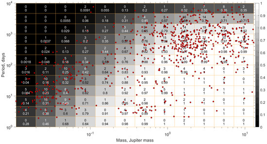
Figure 1.
The detectability window W in the form of a map in the m–P plane obtained with the coefficients γ = 0.8 and δ = 2.0 in (5a) and (5b). The upper and lower numbers in each of the cells (Δm, ΔP) present the number of known planets with the minimum mass and the orbital period in the corresponding interval and the probability of detecting planets with these parameters, respectively. The degree of shading a cell corresponds to the detection probability for this cell according to the scale on the right. The red dots show the positions of actually detected RV planets in the m–P plane.
However, the detectability window proposed above by the W matrix is not constructed for all observed stars but only for stars with planets. Therefore, the correction by W is neither complete nor accurate, as it does not account for possible low-mass planets orbiting stars by which no planets have been detected.
Without loss of generality, we can relax this inconsistency by the following algebra.
We consider L- number of observation programs (surveys), where: The 1-st one can only detect the heaviest of the artificial planets with minimum mass m1; The 2-nd survey detects planets with masses: m1 and m2 (m1 > m2); etc.; Finally, the L-th survey is able to detect planets of all masses: m1, m2, …, mL. Assume, the 1-st survey observes N*1 stars, the 2-nd—N*2 stars, etc., the L-th survey—N*L stars. The corresponding occurrence rates of planets with masses m1, m2, …, mL are denoted by f1, f2, …, fL.
Logically, the 1-st survey finds f1∙N*1 planets with mass m1, the 2-nd survey finds f1∙N*2 planets with mass m1 and f2∙N*2 planets with mass m2, and so on, until the L-th survey detects f1∙N*L planets with mass m1, f2∙N*L planets with mass m2, …, fL∙N*L with mass mL.
Counting the number of detected planets results in: The heaviest planets with mass m1 will be detected f1∙N*1 + f1∙N*2 + … + f1∙N*L = f1∙(N*1 + N*2 + … + N*L) times. The number of planets with m2 mass is f2∙(N*2 + … + N*L). Finally, the number of lightest planets with mL mass is fL∙N*L.
However, it is important that in reality, the quantity of planets with m1 mass will be f1∙(N*1 + N*2 + … + N*L), the quantity of planets with m2 mass will be f2∙ (N*1 +N*2 + … + N*L), and so on, and the quantity of mL mass planets will be fL∙ (N*1 +N*2 + … + N*L).
To convert the observed numbers of planets into their real numbers, the detection efficiency values (elements of the detectability window matrix V(←W)) shall be following:
v1 = 1, (for planets with m1 mass);
…
In other words, each coefficient of the detectability window matrix V is the ratio of the sum of stars in which a planet with a given minimum mass and orbital period can be detected to the total sum of all observed stars.
Directly from the NASA Exoplanet Archive [1], we know neither the number of observed stars in each artificial survey N*i nor the occurrence rates of planets fi in the mass domain between mi−1–mi+1. However, instead, we do know the number of stars with detected planets of masses m1, m2, …, mL. The number of stars that have the planets detected in the i-st survey (denoted as) Si:
S1 = d1·f1∙N*1, (detected by the 1-st survey);
S2 = d2 · (f1∙N*2 + f2∙N*2) =
= d2·N*2 (f1 + f2), (detected by the 2-nd survey);
= d2·N*2 (f1 + f2), (detected by the 2-nd survey);
…
SL = dL·N*L…(f1 + f2 + … + fL), (detected in the L-th survey).
By definition, the coefficient di is the ratio of the number of stars to the number of observed planets orbiting these stars. For small f, the coefficient d is close to 1 (as a rule, a star has only one known planet), but as f increases, d decreases, and it tends to the value inverse to the average number of planets per star. For giant planets of 2–13 Jupiter masses considered in this paper, d = 0.931 (248 planets in 231 stars), and for planets with masses less than 0.1 Jupiter masses d = 0.676 (145 planets in 98 stars). To exclude the additional factor d, when constructing the detectability window matrix for a multiplanet system we further consider the star as many times as it has known planets. In this case, Equation (7) can be re-written as:
…
It follows from the statements above, that is possible to re-write the detectability window matrix (see below (9a)–(9c)) that accounts only for detected planets, into the detectability window matrix V, which takes into account all the observable stars (6a)–(6c). One can realize that had the matrix elements 1…L along the minimum mass m direction, which are:
…
The corresponding Formulas (6a)–(6c) and (9a)–(9c) for vi and i are structurally identical, but they have the different N*i and i metrics, where N*i counts observed stars, while i counts detected planets.
We further express i through the matrix elements i (from (8b));:
From (8a)–(8c), we express the number of observed stars N*i through the number of the planets detected in the i-st survey i:
Finally, vi is found via i:
…
For example, if fi = constant (that makes “flat” distribution on a logarithmic scale , corresponding to the mass distribution ∝ m−1), then / = i/j.
If dN/dlog m ∝ m−α (which corresponds to the mass distribution of ∝ m−α−1), fi = f1·mstepi−1,
where mstep is (mi/mi+1)α.
Without knowing N*i (which defines the total number of observed stars in each survey, including those without planets), we cannot determine the fi occurrence rate. However, since fi enters expressions for vi only as relations of the form /, we can compute vi by restoring the distribution of planets by mass i, by a f(m) guess, as a function of planetary mass in a fixed orbital period domain.
Examples of detectability windows (for multiplanet systems) and (for stars with and without planets) are shown in Figure 2a,b, respectively.
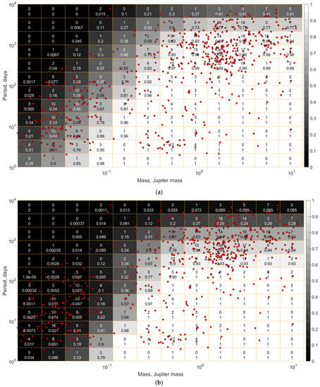
Figure 2.
The detectability windows: (a)
(for multiplanet systems) and (b) (for stars with and without planets) in the format of maps in the m–P plane obtained with the coefficients γ = 0.8 and δ = 2.0. The designations are the same as those in Figure 1.
In aid of understanding, a toy model simplified with L = 2 (with two types of planets observed by two surveys) is discussed and illustrated in Appendix B.
The approach above of Equations (6)–(12) is applicable if all the surveys can be arranged in a monotonic sequence according to increasing (or decreasing) detection efficiency of exoplanets. It is possible if the detection efficiency depends monotonically on only one parameter, e.g., the planet mass m (determined by single condition). However, in the general case, the detection efficiency of exoplanets is a function of several variables, hence, in the present paper, we stretch them to the two major parameters (m, P) in (5). We note that for some set of regions on the plane (m, P), one of the conditions accounting for the survey arranged either along planet mass m or orbital period P as the only parameter is always fulfilled, to make the approach described above (6–12) is applicable. Let us comment that (6)–(12) approach is also applicable by replacing m to P, where it is required. Suitable here one more comment is that all the notations, such as those used by forming the detectability windows V(m, P) (for stars with and without planets, Equation (6)), W(m, P) (accounting for a single planet in systems, Equation (8)) and (m, P) (for multiplanet systems, Equation (8)) can be similarly determined as well for the discrete (centered) mi and Pi values as for their sets collected in intervals Δm = [mi … mi+1] and ΔP = [Pi … Pi+1].
To ensure that the constructed various detectability windows W(m, P), (m, P) (8) and V(m, P) (6) do actually reflect the current ability of the RV technique to detect exoplanets, we should specify the parameters γ and δ (5) more accurately in each mass- and orbital period domain.
2.2.2. Parameters of the Detectability Window Regularization Algorithm
The values initially assumed for the coefficients in (5a) and (5b) (and illustrated in Figure 1 and Figure 2) γ = 0.8 and δ = 2.0, do characterize the majority of discovered planets, the orbital periods of which are longer than the full time of their observations T (e.g., HD 181234 b [21]). Moreover, some planets induce sinusoidal fluctuations in the radial velocity of a host star with a semi-amplitude K smaller than σ(O − C) (e.g., GJ 433 d [22] and HD 26965 b [23]), which implies γ < 1.0.
To determine the coefficient δ, we plot the distribution of RV planets over the ratio P/T in the form of a histogram (see Figure 3).
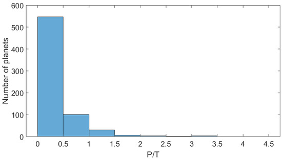
Figure 3.
The distribution of RV planets over the ratio of the orbital period P to the total time of observations T.
According to Figure 3, P/T < 1.5 for the majority of RV-planets (97.7%), and P/T < 2.5 for 99.1% of them. When choosing a value for the coefficient δ, we should take into account that those planets which have passed only a part of their orbit around host stars during the time of observations may also be detected. The smaller the fraction of the orbit the planet has passed, the less reliably its minimum mass and orbital period can be determined. If this fraction of the orbit is small, the Kepler curve degenerates into a linear or quadratic drift of the star’s radial velocity, which indicates the presence of long-periodic bodies in the system, but does not allow their period and mass to be determined. For example, planets with P/T > 2.5 (HD 221420 b, Pr0211 c, HAT-P-17 c, HR 5183 b, HD 190984 b, and HD 133131 B b) are in highly eccentric orbits. During the observational period, they have already passed through pericenters, when the orbital velocity changes rapidly. If the same planets had been observed during their apocenter passages, they would have been apparently missed as a poorly defined source of a linear drift in the radial velocity of their host stars. For most planets with P/T > 2.5, the orbital periods and the semi-major axes of orbits are poorly determined.
It is also worth noting that the variation of the coefficient δ mostly influences the detection probability of planets with the longest periods, while the influence of coefficient δ on the detection probability of short- or medium-period planets is very weak. We will further set δ = 2.0; i.e., we accept the condition that a planet can be detected if it has completed at least a half revolution on the orbit around its host star for the entire period of observations.
Next, let us consider whether it is possible to choose a universal value for the coefficient γ that would be valid for detecting most RV planets so that .
The distribution of RV planets over the ratio K/σ(O − C) in the form of a histogram is shown in Figure 4.
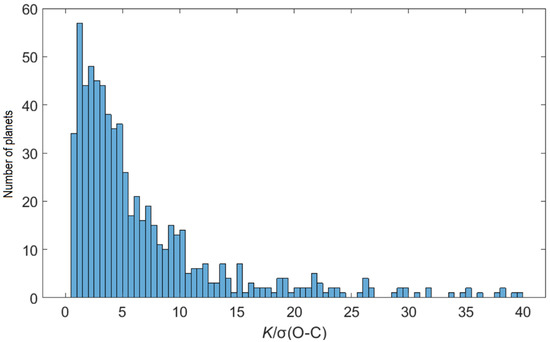
Figure 4.
The distribution of RV planets over the ratio of the semi-amplitude K of the radial velocity oscillations of a host star to the average deviation σ(O − C) from the best Keplerian curve.
For the majority of planets (95.1%), K/σ(O − C) > 1.0, i.e., the semi-amplitude K of fluctuations in the radial velocity of a host star, which are caused by the gravitational influence of the planet, is greater than the average deviation σ(O − C) from the best Keplerian curve. However, for 34 planets out of 695 (4.9%), 0.5 < K/σ(O − C) < 1.0. As a universal approximation, we may set γ = 0.8; although, in Section 3, for each of the intervals of the minimum masses m, optimal values of γ will be chosen.
Nevertheless, the detectability window matrix W (in Figure 1) contains zero probability fp = 0 in the following eight elements (or the map cells with numbers i and j along the horizontal and vertical axes, respectively): W11, W21, W31, W12, W22, W13, W14, and W15. These “degenerate” cells correspond to planets of small masses and large orbital periods. We call this degenerate region “a blind spot”. It is impossible to detect planets from the blind spots (with the corresponding parameters Δmi and ΔPj) even with state-of-the-art tools, and unfortunately, their number remains unknown for constructing statistical patterns.
Note that since for wij = 1 ij = 1 and vij = 1, and for wij = 0 ij = 0 and vij = 0, the blind spot area does not change when moving from the imprecise matrix W to the refined matrix V (see Figure 2).
3. Results
3.1. De-Biased Histograms of the Projective-Mass Distributions of RV Planets
3.1.1. The Technique for Constructing the Projective-Mass Distributions of RV Planets and Their Histograms
We analyze the projective-mass distribution of RV planets N(m) = dN/dm with the example of the detection probability matrices—the detectability windows W, and —shown in Figure 1 and Figure 2a,b, correspondingly.
First, using the detectability windows W (accounting for stars with single planets), we write the numbers of planets N in the map cells (the upper numbers shown in the cells) as the matrix N0(12 × 12) and use Equation (4) to regularize the data and correct the observational selection. To pass from the two-dimensional non-corrected (biased) distribution N0(Δm, ΔP) to the corrected mass distribution of RV planets in the form of a histogram N(m) = dN/dm, we sum up the elements of the matrix N0 × (1/W) (see (4)) by columns, i.e., by orbital periods:
However, in the blind spot (cells W11, W21, W31, W12, W22, W13, W14, and W15), the elements of the matrix N cannot be defined due to the division by zero. Because of this it is impossible to construct a mass distribution for the whole m−P plane, i.e., for i and j both running from 1 to 12. There are two ways to overcome this problem:
(A). We cover the planets of all masses, but limit ourselves to those with short orbital periods, i.e., i = 1–12 and j = 7–12:
(B). We cover planets with all periods, but limit ourselves to more massive planets, i.e., i = 4–12 and j = 1–12:
In Figure 5a,c we show the distribution of planets as a histogram NA(m) for all considered masses with the orbital periods ranging from 1 to 100 days. This distribution was obtained according to Equation (13b) for several values of γ and δ (γ = 0.65, 0.80, 0.95; δ = 1.5, 2.0, 2.5). Figure 5d show the distribution of planets NB(m) for all considered orbital periods and the masses exceeding 0.065 MJ (21ME); it was calculated according to Equation (13c).
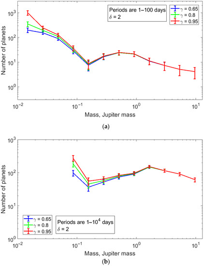
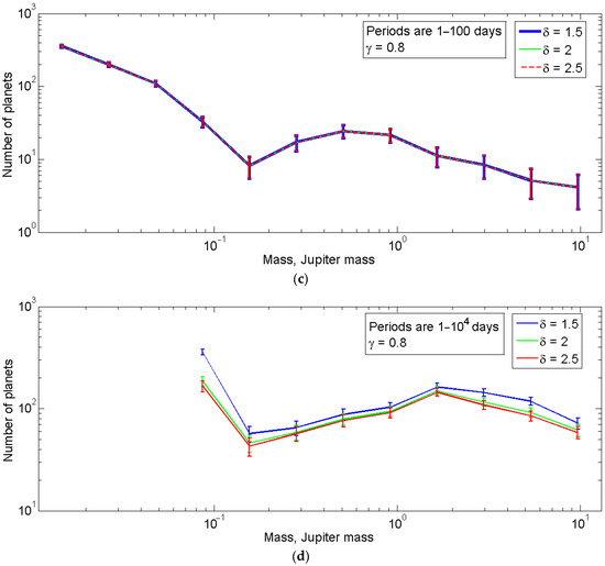
Figure 5.
The corrected (de-biased) mass distributions of planets N(m). The coefficients are set at δ = 2.0 and γ = 0.65, 0.8, and 0.95 for the planets with m = (0.011–13) MJ and P = 1–100 days (panel (a)) and with m = (0.065–13) MJ and P = 1–104 days (panel (b)). The coefficients are set at δ = 1.5, 2.0, and 2.5 and γ = 0.8 for the planets with m = (0.011–13) MJ and P = 1–100 days (panel (c)) and with m = (0.065–13) MJ and P = 1–104 days (panel (d)). The error bars were estimated according to the Poisson distribution.
When passing from the integer numbers of planets N0 in Equation (6a) (see the upper numbers in the map cells in Figure 1) to the fractional numbers of planets N in Equations (6b) and (6c), we took into account the error in determining planetary masses by the kernel density estimation (KDE). In this procedure, we used a Gaussian profile or a skewed normal distribution, depending on whether the upper and lower errors are equal (the smoothing technique was described in [24] and presented at length by [25]) or differ in magnitude [26], respectively.
As a first approximation, the mass distribution of RV planets in Figure 5 follows a piecewise continuous power law with breakpoints approximately located at 0.14 MJ and 1.7 MJ (see Figure 5b,d for more precise positions). It is important that the breakpoint positions are independent of selected values of the coefficients γ and δ. The breakpoint positions are determined within an accuracy of the bin width in the histogram.
It should be noted that the projective-mass distribution for planets with periods of 1–100 days significantly differs from that for planets with periods of 1–104 days even in the projective-mass domain, which is common for the both distributions (i.e., (0.063–13) MJ). While the positions of minima (0.14 MJ) coincide in the both distributions, the positions of the maxima are different (~0.5 MJ and ~1.7 MJ for the short-periods planets and the planets with all periods observed, respectively). As it will be shown in Section 4, this suggests that the most massive planets are on wide orbits with periods exceeding 100 days.
As can be seen in Figure 5c, the distribution of planets with periods of 1–100 days does not depend on the choice of the value for δ either (the distributions are the same for δ = 1.5, 2.0, and 2.5). This is due to the fact that, for short-period planets, the whole time of observations always exceeds their orbital periods, i.e., P/T < 1.
Let us state that the breakpoint positions at 0.14 MJ and 1.7 MJ do not depend on the values of the coefficients γ and δ. The slopes of the mass distributions of planets in three mass intervals slightly depend on γ choice. Therefore, we better determine the parameters γ and the power indices α (in N(m) ∝ m−α approximation) in each of the mass intervals. We have analyzed these intervals separately.
The power indices of de-biased mass dependencies within optimal parameters for the intervals between the breakpoint positions are summarized in the Table 1.

Table 1.
Optimal parameters and power law approximation for three mass intervals.
3.1.2. The Composite Projective-Mass Distribution of Planets—Comparison to the Mass Distributions from Population Synthesis Theory
In Figure 4, the projective-mass distribution of RV planets corrected with the detectability window regularization algorithm rather accurately follows a power law piecewise. In a domain of (0.011–0.087) MJ (or (3.5–28)ME), the exponent is −3, i.e., dN/dm ∝ m−3. In a domain of (0.087–0.21) MJ (or (28–67)ME), the distribution exhibits a minimum, which is deepest in a range of (0.12–0.16) MJ (or (37–50)ME), where the number of planets is 7.7 times smaller than that predicted by the power law with an exponent of −3. In a mass domain of (0.21–2.2) MJ, the distribution follows a power law with an exponent ranging from −0.8 to −1, i.e., dN/dm ∝ m−0.8…−1. In a mass domain of (2.2–13) MJ, the distribution may be approximated by a power law with an exponent ranging from −1.7 to −2.0, i.e., dN/dm ∝ m−1.7…−2.0.
Due to the presence of the blind spot (zeroed W11, W21, W31, W12, W22, W13, W14, and W15), it is impossible to plot the mass distribution of RV exoplanets in the entire mass range of 0.011–13 Jupiter masses and orbital periods of 1–104 days. However, we obtained a composite mass distribution of the RV exoplanets by putting on one plot the distribution of light planets (0.011–0.21 Jupiter masses) with orbital periods of 1–100 days and the distribution of medium and heavy planets (0.21–13 Jupiter masses) with orbital periods of 1–3981 days. For greater uniformity, we considered only systems with a noise level σ(O − C) < 15 m/s (598 planets). When constructing the distribution of medium and large masses planets, we considered only systems whose total observational time T exceeded 1990.5 days.
In Figure 6a, we superimpose the overlapping parts for the host stars in the mass domain of the distributions in a range of (0.156–0.378) MJ (the right end of the blue curve and the left end of the green one) by 3.75. The coefficient 3.75 was chosen as the ratio of the number of planets in the mass interval 0.156–0.378 of the Jupiter mass with orbital periods of 1–3981 days and 1–100 days.
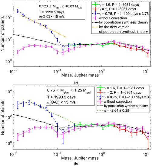
Figure 6.
(a) The composite de-biased (via V) distribution for the minimum masses of 598 RV planets with masses of 0.011–13 Jupiter masses that are part of systems with a noise level σ(O − C) < 15 m/s. For all sections of the distribution, δ = 2.0 was assumed. The blue solid line shows the distribution of planets with orbital periods of 1–100 days (γ = 0.75), the blue dashed line shows the same distribution multiplied by 3.75. The green and red solid lines show the corrected distribution of planets with periods of 1–3981 days with γ = 1.6 and 2.0, respectively. The dotted magenta line shows the biased distribution of RV planets with periods of 1–104 days (from the NASA Exoplanet Archive [1]). The black dashed line shows the distribution of exoplanets by mass predicted by population synthesis theory [2], the orange dotted line shows the distribution of planets with masses 5–50 Earth masses according to the new version of population synthesis theory [3]. (b) The similar dependencies for FGK host stars (with the star masses 1.00 ± 0.25 solar mass).
With the planetary population synthesis, Mordasini (2018) [2] established a theoretical model of the formation and evolution of planets; consequently, the theoretically derived mass distribution of planets may be compared to observations: therefore, both the biased and the de-biased distributions. The predicted mass distribution of planets displayed (by [2] in Figure 10 (top left panel)) is reproduced here in Figure 6 by a dashed black line. In a mass domain of (1–30)ME (or (0.003–0.1) MJ), the distribution follows a power law with an exponent of −2, i.e., dN/dm ∝ m−2. In a mass domain of (0.1–5) MJ, the predicted mass distribution follows a power law with an exponent of −1, i.e., dN/dm ∝ m−1 (which results in a plateau or even a slight increase along the mass bins expressed in logarithm), and in the domain above 5 MJ the power exponent approaches −2 again. The projective-mass distribution of RV planets corrected with the detectability window regularization algorithm is well consistent with the population synthesis theory [2] in the range of 0.21–13 Jupiter masses. However, in the region of masses less than 0.21 Jupiter masses, the corrected distribution does not agree with the distribution predicted in [2]. However, a new generation of population synthesis models (e.g., [3]) predicts a dN/dm ∝ m−3 distribution for planets with masses 5–50 Earth masses. In the mass range 0.087–0.21 MJ there is a deficit of observed planets w.r.t. the theory (the hot Neptunes desert).
In Figure 6b, we analyzed the similar graph as in Figure 6a, but only for FGK host star group in stellar mass domain of 1.00 ± 0.25 Msol. Both graphs show a similarity, but the graph corresponding to solar-like (FGK) host stars shows a decreasing planet number in (0.011–0.02) MJ mass domain. Additionally, the mass distribution slope of planets orbiting FGK host stars fits to m−2.64 ± 0.28 in comparison to m−3 for all planets (orbiting host stars with the masses (0.123–10.8) Msol).
3.1.3. The Minimum in the (0.087–0.21) MJ Domain of Masses
The de-biased projective-mass distribution of RV planets exhibits a contrasting minimum in the mass range (0.087–0.21) MJ. In this range, planets are robustly detected: for planets of lower masses, γ = 0.75, while more massive planets require γ = 1.6. We find reasonable to check whether the observed minimum may be explained by the incorrectly estimated detectability efficiency of planets with masses of (0.087–0.21) MJ, i.e., the incorrectly estimated coefficient γ (the transition from γ = 0.75 to γ = 1.6).
We construct the distribution of RV planets over the ratio K/σ(O − C), i.e., the ratio of the half-amplitude K of the radial-velocity oscillations of a host star to the mean deviation from the best Keplerian curve σ(O − C), for a mass range of (0.087–0.38) MJ (58 planets).
Though it is clear that γ = 0.75 in this domain, we modeled the influence of changes in the coefficient γ on the minimum depth in the projective-mass distribution of RV planets, for which the corrections with γ = 0.75 and 1.6 were used. We considered planets with periods of 1–100 days from systems with a noise level σ(O − C) < 8 m/s. The result is presented in Figure 7a.
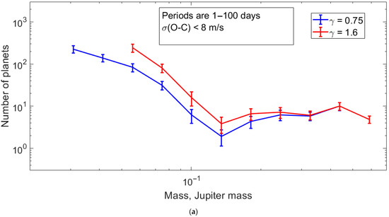
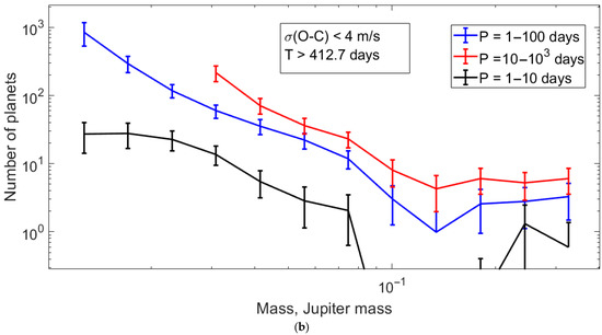
Figure 7.
(a) The de-biased mass distributions of planets with masses m = (0.036–0.38) MJ and orbital periods P = 1–100 days for γ = 0.75 and 1.6. The planets with σ(O − C) < 8 m/s are considered. (b) The de-biased mass distributions of the planets having the orbital periods of 1–100 days (blue line), 10–1000 days (red line), and 1–10 days (black line). The planets of low-noise systems (with σ(O − C) < 4 m/s) are considered. By guess, the minimum is caused by planets in tight orbits.
As can be seen from Figure 7a, changes in the coefficient γ do not basically change the distribution pattern. In the minimum domain ((0.108–0.135) MJ or (34–43)ME), the number of planets predicted by the power law fitting the range of small masses is seven times larger than the number of planets corrected by the detectability window with γ = 0.75. Moreover, the number of planets in the same domain corrected by the detectability window with γ = 1.6 is in 3.6 times smaller than the number of planets predicted by the power law. Consequently, we conclude that the minimum in the (0.087–0.21) MJ range cannot be explained only by a jump in the γ value.
In Figure 7b, we examined the dependence of the distribution of planets by mass, depending on the orbital period coverage: 10–1000 days, 4.64–464 days, 2.15–215 days, and 1–100 days (we used period ranges equal in logarithmic scale and equal to 100). We can see that the minimum becomes deeper as the orbital periods decrease, suggesting that the mass values in the minimum range correspond to the so-called “desert of hot-Neptunes” (e.g., [27,28]).
It seems possible that if planets of all orbital periods were detected, including periods longer than 1000 days, this minimum would completely disappear and the de-biased mass distribution of RV planets would agree with the population synthesis theory. On one hand, we note that adding de-biased distributions 1–10 days and 10–1000 days of Figure 7b (therefore, complete 1–1000 days) will certainly still show a deficit in this mass range. On the other hand, Neptune and Uranus in the Solar system still could not be detected from outside, because of their large orbit, long period, small induced K reflex motion and very low transit probability. Therefore, this issue deserves a more rigorous separate analysis, deleted to future for the time being.
3.1.4. The Maximum in the (6–9) MJ Domain of Masses
The projective-mass distribution of planets with masses in a domain of (1.7–13) MJ can be represented as a sum of the power law and the maximum (bump) in a range of (6–9) MJ (Figure 6a,b). This peculiarity can also be seen in the composite de-biased distribution, the de-biased distribution of planets from low-noise systems (σ(O − C) < 15 m/s) and the biased distribution (the dotted magenta line in Figure 6), because in this domain there is just no-correction, matrix elements equal to 1.
This peculiarity may be explained by the contribution of planets formed due to the gravitational instability in the protoplanetary cloud [29], while the other giants were formed due to the nucleus accretion [30,31]. However, a lengthy discussion of this issue is beyond the scope of this paper.
3.2. Histograms of the Orbital-Period Distributions of RV Planets
In Section 2, we have described how to construct and translate the detectability window matrixes W(m, P), (m, P), and V(m, P), which made it possible to correct the observed two-dimensional histogram N0(mi, Pj) for the distribution of RV planets over the orbital periods and minimum masses and obtain the corrected histogram N(mi, Pj).
To derive the mass distribution of RV planets, we summed the matrix elements over orbital periods. The summation can also be made over masses, which will result in the distribution over orbital periods N(P).
Due to the blind spot (zero elements) in the W, and V matrixes, this summation cannot be made over the entire m–P plane (see Section 3.1). For example, it is possible to construct the distribution of planets NA(P) covering all masses and the orbital periods P = 1–100 days analogously to Equation (13b) or to construct the distribution of planets NB(P) covering all orbital periods and the masses larger than 0.12 MJ (37 ME) analogously to Equation (13c).
To derive the distribution NB(P) we consider the planets with minimum masses m = (0.011–13) MJ and orbital periods P = 1–104 days, also divide each of these domains into 12 bins and sum up the matrix elements over minimum masses starting from the fifth column (i.e., sum up the planets with m > 0. 12 MJ).
To describe the distribution NA(P) more accurately we consider the planets with minimum masses m = (0.011–13) MJ and orbital periods P = 1–104 days, divide each of these domains into 12 bins, and sum up the first 6 the matrix elements over minimum masses, (Figure 8a).
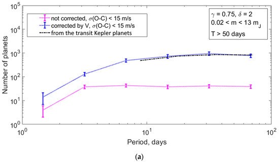
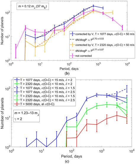
Figure 8.
The orbital-period distribution of RV planets. (a): NA(P) (14a)—de-biased distribution of planets with masses m = (0.02–13) MJ and orbital periods P = 1–100 days for γ = 0.75; the dotted blue line shows the distribution of planets with σ(O−C) < 15 m/s. The orbital-period distribution of the transit Kepler planets with radii of (1–16) RE and orbital periods of 6.25–100 days is shown by black dash-dot line [17]. (b): De-biased NB(P) (14b)—distributions of planets with masses m = (0.12–13) MJ for γ = 1.6: blue line—σ(O − C) < 50 m/s, the orange line—σ(O − C) < 50 m/s, T > 2320 days. The dashed lines in black and brown show approximations by power lows with exponents 0.70 and 0.77, respectively (dN/dlogP P0.70 ± 0.03 and dN/dlogP P0.77 ± 0.07). Initial from NASA Exoplanet Archive [1] (biased) distribution is shown by dotted magenta line. (c): The de-biased distributions of planets with m = (1.2–13) MJ, P = 1–104 days for γ = 2 and δ = 1.5, 2.0, and 2.5. Red line—T > 5000 days, green lines—T > 2320 days and σ(O − C) < 10 m/s, blue lines—T > 1077 days and σ(O−C) < 15 m/s. Solid lines show the distributions corrected by δ = 2.0, dash lines—by δ = 1.5, dotted lines—by δ = 2.5.
We excluded the lightest planets with the masses of 0.011–0.02 masses of Jupiter, because the V matrix values for them are very small (e.g., v(1,6) = 4.9·10−4), while the statistical errors are high. The small number of real planets after the correction becomes very large due to small values of the V matrix elements. In addition, in the region of masses less than five Earth masses (less than 0.016 Jupiter masses), the distribution of planets by masses may not follow the power law with an exponent of degree −3 [3], so the calculation of the V matrix elements made under this assumption becomes incorrect.
For planets with masses m > 0.12 MJ, the planet detection efficiency depends both on the noise level σ(O − C) (affects masses m (5b)) and on the observation duration T (affects periods P (5a)), so we cannot define a final detectability window V(m, P), as described in Section 2.1, (6–12). To construct the distribution of the long-period planets, we can either consider planets discovered by surveys with long observation times T (for them condition (5a) will always be satisfied, and we can apply formalism (6)–(12)), or consider planets of large masses, for which condition (5b) will always be satisfied, and different observation times T. In the latter case, the corrected distribution of the long-period planets will depend on the assumed dependence dN/dP.
Figure 8b shows the distribution of planets with masses 0.12–13 MJ, from the surveys with a total observation time T exceeding 1077 days, here (5a) is satisfied for planets with periods less than 2154 days. The distributions of the planets from the surveys with noise level σ(O − C) < 50 m/s and σ(O − C) < 15 m/s are shown. The obtained distributions display a monotonic increase in the number of planets with increasing orbital periods from 6.8 to 680 days, which can be approximated by a power law with a power index of 0.69 ± 0.03 (dN/dlogP ∝ P0.69 ± 0.03) and 0.70 ± 0.03 (dN/dlogP ∝ P0.70 ± 0.03), respectively.
Moreover, Figure 8b shows the distribution of planets with m = 0.12–13 MJ with a total observational time exceeding 2320 days and noise level σ(O − C) < 50 m/s, planets with P < 4640 days obey the condition (5a). In the range of P = 6.8–680 days, this distribution can be approximated by dN/dlogP ∝ P0.77 ± 0.07, whereas in the range of P = 680–4640 days it becomes flat (dN/dlogP ≈ 0). For comparison, the biased distribution (from the NASA Exoplanet Archive [1]) of planets with m = 0.12–13 MJ discovered by surveys with any total observation time T = 40–11,314 days is shown.
The choice of the coefficient δ in (5a) affects the distribution on the orbital period distribution only in the region of periods δ times the total observing time T. To avoid this uncertainty associated with the choice of δ, we consider only planets discovered by surveys with long observing times T, but they are few. Thus, the number of planets discovered by surveys with a total observation time T > 5000 days is 107 out of 695. To cover as many planets as possible, we considered (i) planets discovered by surveys with full observing time T > 2320 days and noise level σ(O − C) < 10 m/s (316 planets), and (ii) planets discovered by surveys with full observing time T > 1077 days and noise level σ(O − C) < 15 m/s (523 planets). In this case, for planets with m=1.2–13 MJ condition (5b) is always fulfilled (i) for planets with P < 4640 days, (ii) for planets with P < 2154 days.
Figure 8c shows the orbital period distributions for planets m = 1.2–13 MJ (columns 9–12), at different values of the parameter δ (δ = 1.5, 2.0, 2.5) and the minimum total observation time T (T > 1077, 2320, 5000 days).
From Figure 8c, one cannot draw conclusions about the distribution of the planets over orbital periods of more than twice the minimum total observing time since, in this region, the type of distribution is strongly influenced by choice of coefficient δ. Nevertheless, all three distributions in Figure 8c show similar behavior: in the region of periods of less than 46.4 days, there are very few or no planets of 1.2–13 Jupiter masses, in the region of 46.4–464 days, there is a steady increase in the number of planets, in the region of 464–4640 days the distribution becomes flat. There is a hint of a decrease in the number of planets in the last bin (4640–104 days), but it is not yet clear how much of this decrease is real and how much is caused by the observational selection.
The de-biased orbital-period distributions of RV planets were compared to the distribution of the Kepler planets with radii of (1–16) RE and orbital periods of 6.25–100 days [17], it is shown by a dash-dotted black line (Petigura et al. (2013) [17] reduced the orbital-period distribution to a single star, i.e., it represents the occurrence rate. To pass from the occurrence rate to the distribution, one should multiply it by a constant, which is equivalent to a vertical shift). As can be seen from Figure 8a, the orbital-period distributions of the Kepler planets and the RV planets are in good agreement in a domain of 6.25–100 days.
We compared the de-biased orbital-period distributions of RV planets with a similar distribution of Kepler planets with periods of 1–300 days from [6], Figure 12, and found good agreement. The distribution of planets with radii (1–16) RE (shown by the black line in Figure 12 in [6]) looks similar to the blue dotted line in Figure 8a, and the distribution of planets with radii (8–16) RE (shown by the red line in Figure 12 in [6]) looks similar to the distribution of planets with masses (0.12–13) MJ in Figure 8b.
We compare the result in (Figure 8b,c) with ([32], Figure 2), which is based on the orbital period distribution of 155 RV planets with masses of 0.1–20 MJ orbiting 822 stars detected by HARPS and CORALIE. In the range of 7–1000 days, there is a similar increase in the number of planets, which transitions to a roughly flat distribution in the ~1000–4000 day range. For planets with periods in the range of 4·103–104 days [32] show a sharp decrease in the number of planets. Figure 8c does not show such a strong decrease. Perhaps the observed decrease in [32] is due to the reduced detection efficiency of light gas giants (0.1–0.3 MJ) with large orbital periods. The semi-amplitude of their induced radial velocity K is less than ~3 m/s (for stars of Solar mass), and such planets are not detected in most cases.
Since the projective-mass distribution of RV planets exhibits different behavior in mass domains of (0.011–0.14) MJ, (0.14–1.7) MJ, and (1.7–13) MJ, we constructed the orbital-period distributions for the planets from each of these mass domains (Figure 9).
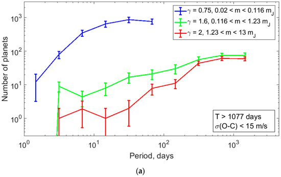
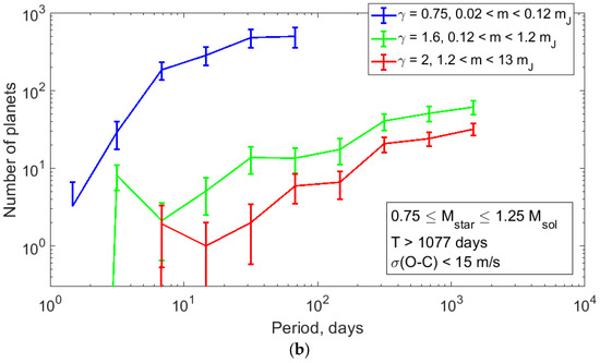
Figure 9.
The de-biased orbital-period distributions for the planets from mass domains of (0.02–0.12) MJ, (0.12–1.2) MJ, and (1.2–13) MJ are shown by blue, green, and red lines, respectively. Planets with a total observation time T > 1077 days in systems with a noise level σ(O − C) < 15 m/s are represented. (a) All types of host stars were considered, (b) FGK host stars were considered.
Figure 9 shows that the orbital-period distributions of planets with small, intermediate, and large masses ((0.02–0.12) MJ, (0.12–1.2) MJ, and (1.2–13) MJ) differ from each other, which suggests a dominating structure of planetary systems. The most massive planets, with m > 2.2 MJ, are mainly on wide orbits with orbital periods longer than 100 days. Only 18 (7.9%) out of 227 massive planets have orbital periods shorter than 100 days. The analogous portion of planets with intermediate masses is 65/233 = 27.9%. The distribution of planets with intermediate masses exhibits a two-fold peak in a range of 2.15–4.64 days, which is not observed in the distributions of planets with small and large masses.
Both distributions of planet numbers versus orbital period agree well within error bars.
We compared the de-biased orbital-period distributions of RV planets with masses of (0.02–0.12) MJ (Figure 9, blue line) with the same distribution of Kepler planets with radii (1–6) RE from ([33], Figure 15, top panel). Although the two sets of planets considered do not match completely, we found good agreement between both distributions (a rapid increase in the number of planets as orbital periods increase from 1 to 10 days and then an approximately flat distribution for orbital periods of 10–100 days).
We compared the de-biased orbital-period distributions of RV planets with masses of (0.02–0.12) MJ with the distribution of Kepler planets with radii (1.7–4) RE (Sub-Neptunes) with periods 1–300 days from ([34], Figure 7) and also found good agreement. The distribution of planets with radii (8–24) RE (Jupiters) and periods 1–300 days from [34] agrees with the distribution of planets with masses (1.23–13) MJ inside the matched interval of orbital periods we obtained.
For this analysis, the detectability matrices W, were calculated by δ = 2.0 for all planets and γ = 0.75, 1.6, and 2.0 for planets with small, intermediate, and large masses, respectively, same for FGK host stars. Matrix V was calculated assuming that the distribution of the masses of the light planets follows the power law dN/dm ∝ m−3, the medium-mass planets follow dN/dm ∝ m−1, and the heavy planets follow dN/dm ∝ m−2. Heavy planets do not require any correction because the corresponding matrix elements were equal to 1.
4. Discussion and Conclusions
The observed distributions of RV exoplanets over minimum masses m = M· sini and orbital periods P were initially distorted (biased) by the observational selection. We have corrected important selection factors as caused by differences in the sensitivity of spectrographs, the activity level of host stars, the mass of the host star, and the duration of the surveys. The results presented here on the mass and period distributions of planets are related to the particular (observed) mass distribution of the 547 stars. Their choice was eventually mixed over different host star types, it may not be well representative of the true and full star distribution in the Galaxy. The overall distribution of planetary masses and periods of the host stars of all types can be artificial because the host star mass or its spectral class possibly determines a planetary interior to be compact or Solar system close analogue or different.
Separately we have considered planets distribution of FGK host stars in stellar mass domain of Mstar = 1.00 ± 0.25. Most of the host stars of the known RV planets are sun-like.
Evidently, the mass distribution of transiting planets can be dependent on the spectral class of their parent stars. However, if the giant planets in stars of spectral classes F, G, K were considered in [8], a certain independence was shown.
To account for the observational selection, the “detectability window” regularization algorithm was used. The method is based on a concept of the detectability window matrix V(m, P) in the m−P plane, the components of which are determined as the probabilities of detecting planets in each of the intervals of minimum masses and orbital periods. When constructing the corrected distributions over minimum masses and orbital periods in the form of a histogram, each detected RV planet was accounted for with a statistical weight inverse to the value of the V matrix component for specified values of P and m.
We considered planets with minimum masses m = (0.011–13) MJ (or (3.5–4131)ME) and orbital periods P = 1–104 days. Within these limits, some elements of the V matrix contain zeros, which means that planets of low masses and large orbital periods cannot be detected. We obtained the distributions of planets with all masses and orbital periods of 1–100 days (Equation (13b)) or the distributions of planets with all orbital periods and masses larger than 0.12 MJ (Equation (13c)).
The composite projective-mass distribution of RV planets obeys a piecewise power law with two breakpoints at ~0.12 MJ and ~2.2 MJ (Figure 6). The distribution of RV planets with m = (0.02–0.087) MJ (or (6.3–28)ME) follows a power law with an exponent of −3, dN/dm ∝ m−3. The distribution of RV planets with m = (0.21–2.2) MJ follows a power law with an exponent ranging from −0.8 to −1.0, dN/dm ∝ m−0.8…−1.0. The distribution of RV planets with m = (2.2–13) MJ is fitted by a power law with an exponent ranging from −1.7 to −2.0, dN/dm ∝ m−1.7…−2.0. In general, the composite projective-mass distribution of RV planets partly agrees with the predictions of the population synthesis theory [2,3].
At the same time, the corrected projective-mass distribution exhibits some peculiarities. In a mass domain of (0.087–0.21) MJ (or (28–67)ME), there is a minimum, the depth of which exceeds a 7.7-fold for planets with P = 1–100 days and m = (0.11–0.14) MJ (or (34–43)ME).
When considering samples of planets with large orbital periods, this minimum becomes smaller and just disappears for planets with orbital periods of 10–1000 days (Figure 7b). We assume that this minimum is caused by a lack of this kind of planets in tight orbits and corresponds to the so-called desert of hot Neptunes [27,28].
In a mass domain of (6–9) MJ, the distribution of RV planets exhibits a maximum. Probably, this maximum appears due to the contribution of planets formed due to the gravitational instability in the protoplanetary disk, while the other giant planets were formed due to the core accretion.
We have directly compared true mass distributions (from theory of formation [2,3]) with observed minimum mass distributions. Is this legitimate? If the true mass distribution follows a power law with exponent α, does the minimum mass distribution has the same exponent α? and vice-versa? To the best of our knowledge, this question has not yet been cleared in the literature. However, using a particular geometrical representation of an ensemble of exoplanets, Bertaux et al. (2021) [35] have shown that this is indeed the case. In addition, Bertaux et al. (2021) have performed forward simulations of true mass distributions for various values of a power law exponent, giving minimum mass distributions. They were then fitted by a power law. For a true mass distribution with a power law with exponents α = −1.5, α = −2, and α = −2.5, we found, respectively, for the minimum mass distribution: −1.57, −2.03, and −2.498. The small differences are due to edge effects. Therefore, we think it is fully legitimate to compare directly the exponents of power laws of a true mass distribution (coming from theory) and an observed minimum mass distribution (See also [4,36]).
We also analyzed the orbital-period distributions of planets. Due to the blind spot, the distribution of RV planets cannot be obtained for the entire m−P plane. We derived the orbital-period distribution of planets with masses of (0.02–13) MJ with P = 1–100 days and the distribution of planets with all considered orbital periods but with masses exceeding 0.12 MJ.
The de-biased distribution of planets with masses (0.02–13) MJ and orbital periods of 1–100 days displays a rapid increase in the number of planets with increasing periods from 1 to 10 days and a close to flat distribution in the region of 10–100 days. The distribution shape is well consistent with that for the Kepler (transiting) planets with radii of (1–16) RE and orbital periods of 6.25–100 days [6,17,33]).
The distribution of planets with masses larger than 0.12 MJ (37 ME) shows a local maximum at P = 2.15–4.64 days. In the domain of 6.8–680 days, the distribution follows a power law with an exponent of −0.3 (dN/dP P−0.3), in the region of 680–4640 days the distribution becomes flat (dN/dP P−1) (Figure 8b,c). The orbital-period distributions of RV planets from three mass domains, where the projective-mass distributions behave differently ((0.02–0.12) MJ, (0.12–1.2) MJ, and (1.2–13) MJ), also differ (Figure 9). Specifically, most massive planets, with m > 2.2 MJ, are mainly on wide orbits with orbital periods longer than 100 days. This may suggest that there is a prevailing structure of planetary systems, within which low-mass planets are on orbits close to host stars, while massive planets are on wide orbits, analogous to the situation in the Solar System.
Author Contributions
Conceptualization, V.A.; methodology, V.A.; software, O.Y.; validation, O.K. and J.-L.B.; investigation, V.A.; resources, V.A. and A.I.; data curation, V.A.; writing—original draft preparation, I.S.; writing—review and editing, V.A. and A.T.; visualization, I.S.; supervision, A.T. All authors have read and agreed to the published version of the manuscript.
Funding
The authors acknowledge the support of Ministry of Science and Higher Education of the Russian Federation under the grant 075-15-2020-780 (N13.1902.21.0039).
Conflicts of Interest
The authors declare no conflict of interest.
Appendix A. Method for Merging Together Several Surveys
Let us consider one particular RV survey of exoplanets containing N stars, with its own sensitivity and duration. Within a particular bin (Δm,ΔP), this survey detected fobs(Δm,ΔP), while the exercise of checking the “detectability” of a dummy planet (m, P) around all N stars yielded N fp(Δm,ΔP). Therefore, we can say that the true occurrence rate focc(Δm,ΔP) of this type of planet around stars, in units of “planets per star”, is given by:
This is exactly the Equation (13) of Tuomi et al. (2019) [16].
We can describe this Equation (A1) by stating that the occurrence rate of planets in a certain bin is simply the ratio of the number of actually detected planets to the number of “detectable” planets, given the particular characteristics of the survey (accuracy of RV, period covered).
Now, we describe how can be simply merged the results of two surveys S1 and S2 with different sensitivity ((O − C) threshold), different durations (which will impact the coverage of periods) and different numbers of planets monitored, respectively, n1 and n2. Let us call q1 and q2 the number of “detected” dummy planets in the bin (Δm, ΔP). We have, by definition of fp(Δm,ΔP):
q1 = n1 fp1(Δm,ΔP); q2 = n2 fp2(Δm,ΔP)
Therefore, we have two estimates of the occurrence rate of planets (m, P) focc(Δm,ΔP):
focc1(Δm,ΔP) = fobs1(Δm,ΔP)/q1 ; focc2(Δm,ΔP) = fobs2(Δm,ΔP)/q2
In order to obtain an estimate from the combination of the two surveys, one could make an average of focc1(Δm,ΔP) and focc2(Δm,ΔP), or some kind of weighted average. However, there is a simpler way to obtain a combined estimate. Indeed, we note that (dropping ((Δm,ΔP) for simplicity):
The numerator of the last fraction is simply the sum of the planets detected in the two surveys. The denominator is the sum of dummy planets detected (detectable planets) in the two surveys. This can be extrapolated to any number of surveys with different characteristics, and we can state:
Regardless of the different characteristics of the various surveys, the (true) occurrence of planets (number of planets per star) in a certain bin is simply the ratio of the total number of actually detected planets in all surveys to the total number of “detectable” planets in all surveys, when detectability is computed for each survey given the particular characteristics of each survey (accuracy of RV, period covered).
and therefore the true number of planets N(m,P) in this bin for all Q stars (Q = (547 in the present study) of the combined surveys is:
We then define the detectability window for a particular bin as:
and therefore the true number of planets N(m, P) in this bin for all Q stars of the combined survey is:
Coming back to one particular single survey, Figure A1 is a sketch of the Detectability window in a diagram Period P/amplitude K of the reflex motion of a star influenced by the presence of one planet around the host star. The solid lines result from Equation (2) for a planet of 0.1 MJ and two masses of the host star. Within a given survey, the planet will be or will not be detected according to the mass of the host star and the sensitivity limit of the survey.

Figure A1.
This is a sketch of the Detectability window, in a diagram of observables in one RV survey: the period and the amplitude K (m/s) of a sinusoidal variation of RV induced by a planet. The two solid lines represent the relation for a planet of 0.1 MJ around a host star with 1 solar mass (red) and 0.1 solar mass Msun (black). The same planet will be detected around a host star with mass 0.1 Msun and not detected around a host star with mass 1 Msun. The rectangular blue-shaded area represents the area of the detectability window; γ and δ are two multiplicative factors affecting the boundaries of the detectability window that can be adjusted simultaneously to all surveys, for a more homogeneous treatment (see text).
Appendix B
Here we discuss an artificial example in which only two types of planets are considered: the heavy (1) and light (2) planets. Their occurrence rates are f1, f2, correspondingly. We consider, therefore, two surveys, the first can detect only heavy planets, and the second can detect all the planets. Let the first survey observe N1 stars, while the second survey observe N2 stars.
The first survey detects f1·N1 heavy planets and zero light planets. The second survey detects f1·N2 heavy planets and f2 ·N2 light planets. The number of heavy planets detected is f1·N1 + f1·N2 = f1·(N1 + N2). The number of light planets detected is f2 ·N2.
However, the true number of light planets orbiting all observed stars is f2 ·(N1 + N2).
For de-bias, the detectability window matrix V consists of the following 2 cells:
| v2 | v1 |
Here v1 = 1 (means that all surveys detect the heavy planets), v2 = (f2 ·N2)/(f2 ·(N1 + N2)) = N2/(N1 + N2).
| N2/(N1 + N2) | 1 |
To check and visualize it we assume some casual numeric, f1 = 0.05, f2 = 3, N1 = 1000, N2 = 20. Then the first survey detects f1·N1 = 50 heavy planets. The second survey detects f1·N2 = 1 heavy planets and f2 ·N2 = 60 light planets. The total number of detected heavy planets is f1·N1+ f1·N2 = 51, the total number of detected light planets is 60. However, while the true number of light planets is f2 ·(N1 + N2) = 3060.
If one corrects the number of light planets by v2 = N2/(N1 + N2) = 20/1020 = 1/51, then resumed the corrected number of light planets is f2 ·N2/v2 = 60/(1/51) = 3060.
From here we complicate our de-biasing technique a bit, we assume we do not know the numbers of observed stars in surveys: N1 and N2 (e.g., due to the lack of a proper criterion of planet non-detection). However, oppositely, we know the numbers of the stars denoted by S1 and S2 with detected planets corresponding to the surveys.
The first survey detects f1·N1 heavy planets orbiting S1 = d1·f1·N1 stars, the second survey detects f1·N2 heavy planets and f2 ·N2 light planets orbiting S2 = d2·N2·(f1 + f2) stars. The coefficient di defines the ratio of the number of stars to the number of observable planets in those stars. For small fi di→ 1 (for small fi every star with planets has only one planet). For big fi Si→ Ni (every observed star has planets).
The detectability window matrix W also consists of 2 cells:
| w2 | w1 |
w1 = 1.
w2 = S2/(S1 + S2) = 1/(1 + S1/S2).
If S1 = 50, S2 = 20, than w2 = 2/7.
The corrected number of light planets is 210. Thus, one counts only stars with planets results in underestimate the number of light planets.
We express S1/S2 through w2: S1/S2 = 1/w2 − 1.
We express Ni through Si: N1 = S1/(d1·f1), N2 = S2/(d2·(f1 + f2)).
Than v2 = N2/(N1 + N2) = 1/(1 + N1/N2) = 1/(1 + S1/S2·d2/d1·(f1 + f2)/f1) =
= 1/(1 + (1/w2 − 1)·d2/d1·(f1 + f2)/f1).
In order to exclude the unknown factors di, further we consider the star as many times as the number of the orbiting planets are known, that in the case of a multiplanet system when constructing the detectability window matrix: W(S) → Ŵ(Ŝ). Then Ŝ1 is the number of planets detected by the first survey and Ŝ2 is the number of planets detected by the second survey.
N1 = Ŝ1/f1,
N2 = Ŝ2/(f1 + f2), and
v2 = N2/(N1 + N2) = 1/(1 + (1/ŵ2 − 1)·(f1 + f2)/f1).
To calculate v2 through ŵ2, we have to know the relation f2/f1.
In our case f2/f1 = 60 and (f1 + f2)/f1 = 61.
Let us check it out.
ŵ2 = Ŝ2/(Ŝ1 + Ŝ2) = 61/(50 + 61) = 61/111
v2 = 1/(1 + (111/61 − 1)·61) = 1/51.
Finally, we have to estimate the unknown ratio f2/f1. We consider it from the ratio of light and heavy planets discovered by second survey Ŝ2/Ŝ1. If one underestimates f2/f1, (e.g., accepts f2/f1 = 50 and (f1 + f2)/f1 = 51), then the number of light planets is underestimated: v2 = 1/(1 + (111/61 − 1)·51) ≈ 0.0234, and the corrected number of light planets is 2568. If one overestimates f2/f1, (e.g., accepts f2/f1 = 70 and (f1 + f2)/f1 = 71), then the number of light planets is overestimated: v2 = 1/(1 + (111/61 − 1)·71) ≈ 0.0169, and the corrected number of light planets is 3558. Let us claim that these inaccuracies are not critical.
Figure A2 shows the ratio between w2 и v2 depending on the f2/f1. The Table A1 shows de-biased number of light planets by applied method (by W and by V).

Figure A2.
The ratio between w2 и v2 versus of f2/f1.
Table A1.
De-biased number of light planets depending on applied method (W or V matrices).
Table A1.
De-biased number of light planets depending on applied method (W or V matrices).
| Parameters | Low-Mass Planets | Intermediate Masses | Massive Planets |
|---|---|---|---|
| Without correction | 60 | 3060 | 51 |
| Correction by W | 210 | 14.57 | |
| Correction by V (true f2/f1) | 3060 | 1 | |
| Correction by V (underestimated f2/f1) | 2568 | 1.19 | |
| Correction by V (overestimated f2/f1) | 3552 | 0.86 |
Table A2.
List of considered RV planets (shading at FGK stars).
Table A2.
List of considered RV planets (shading at FGK stars).
| N | Planet Name | Orbital Period, Day | Span, Day | Planet Mass, MJ | Host Star Mass, m☉ | σ(O-С), m/s | RV K, m/s |
|---|---|---|---|---|---|---|---|
| 1 | HD 24064 b | 535.6 | 1921 | 1.61 | 34.5 | 251.00 | |
| 2 | HATS-59 c | 1422 | 1742 | 1.038 | 100.00 | 224.00 | |
| 3 | BD+20 2457 c | 622 | 1833 | 10.83 | 60.00 | 160.03 | |
| 4 | HD 87646 b | 13.481 | 2500 | 1.12 | 270.00 | 956.00 | |
| 5 | HIP 67537 b | 2556.5 | 4419 | 2.41 | 8.00 | 112.70 | |
| 6 | HD 220074 b | 672.1 | 1374 | 1.2 | 57.40 | 230.80 | |
| 7 | HD 110014 b | 835.477 | 2950 | 2.17 | 45.80 | 158.20 | |
| 8 | HD 106270 b | 2890 | 1484 | 1.32 | 8.40 | 142.10 | |
| 9 | HD 13189 b | 471.6 | 1300 | 2.24 | 54.50 | 173.30 | |
| 10 | TYC 4282-00605-1 b | 101.54 | 1200 | 0.97 | 23.02 | 495.20 | |
| 11 | HD 114762 b | 83.915 | 6901 | 0.8 | 27.40 | 612.50 | |
| 12 | HD 156846 b | 359.51 | 2686 | 1.38 | 6.06 | 464.30 | |
| 13 | HD 95127 b | 482 | 2929 | 3.7 | 50.90 | 116.00 | |
| 14 | 18 Del b | 993.3 | 1772 | 2.3 | 15.40 | 119.40 | |
| 15 | HD 17092 b | 359.9 | 1200 | 6.73 | 16.00 | 82.40 | |
| 16 | HD 39091 b (pi Men b) | 2093 | 6570 | 1.094 | 5.50 | 192.60 | |
| 17 | TYC 1422-614-1 c | 559.3 | 3651 | 1.15 | 18.94 | 233.00 | |
| 18 | HD 208527 b | 875.5 | 1352 | 1.6 | 39.30 | 155.40 | |
| 19 | HD 156279 b | 131.05 | 254.2 | 0.95 | 9.08 | 578.00 | |
| 20 | HD 162020 b | 8.428 | 842 | 0.75 | 13.60 | 1813.00 | |
| 21 | Kepler-94 c | 820.3 | 800 | 0.81 | 13.90 | 262.70 | |
| 22 | BD-13 2130 b | 714.3 | 1529 | 2.12 | 18.30 | 137.60 | |
| 23 | HD 139357 b | 1125.7 | 1287 | 1.35 | 14.14 | 161.20 | |
| 24 | HD 221420 b | 22482 | 6500 | 1.67 | 3.93 | 54.70 | |
| 25 | HD 38801 b | 685.25 | 1143 | 1.207 | 11.00 | 197.30 | |
| 26 | HD 141937 b | 653.22 | 882 | 1.09 | 8.70 | 234.50 | |
| 27 | HD 106515 A b | 3630 | 4800 | 0.97 | 9.63 | 158.20 | |
| 28 | WASP-8 c | 4323 | 2099 | 1.34 | 2.91 | 115.00 | |
| 29 | HIP 63242 b | 124.6 | 1025 | 1.54 | 23.70 | 287.50 | |
| 30 | HD 33564 b | 388 | 417 | 1.25 | 6.70 | 232.00 | |
| 31 | HD 23596 b | 1561 | 2100 | 1.47 | 9.20 | 127.00 | |
| 32 | HD 175167 b | 1290 | 1828 | 1.37 | 6.91 | 161.00 | |
| 33 | HIP 75458 b (iota Dra) | 511.1 | 678 | 1.05 | 10.00 | 307.60 | |
| 34 | HD 1690 b | 533 | 2547 | 1.86 | 29.00 | 190.00 | |
| 35 | gam 1 Leo b | 428.5 | 2195 | 1.23 | 43.00 | 208.30 | |
| 36 | HD 30177 b | 2527.8 | 6300 | 1.053 | 10.00 | 125.98 | |
| 37 | HD 156279 c | 4191 | 4225 | 0.93 | 2.20 | 110.20 | |
| 38 | HD 191806 b | 1606.3 | 3616 | 1.14 | 10.00 | 140.50 | |
| 39 | HD 181234 b | 7462 | 6794 | 1.01 | 20.00 | 126.80 | |
| 40 | HD 222582 b | 572.38 | 683 | 1.12 | 3.36 | 276.30 | |
| 41 | HD 89744 b | 256.78 | 5186 | 1.86 | 16.40 | 269.66 | |
| 42 | HD 104985 b | 199.505 | 1932 | 2.3 | 26.60 | 166.80 | |
| 43 | HIP 105854 b | 184.2 | 1279 | 2.1 | 23.60 | 178.10 | |
| 44 | HD 102329 b | 778.1 | 1484 | 3.21 | 7.20 | 84.80 | |
| 45 | HD 74156 c | 2473 | 3408 | 1.238 | 12.8 | 116.50 | |
| 46 | HD 178911 B b | 71.484 | 3392 | 1.24 | 9.10 | 343.30 | |
| 47 | bet Cnc b | 605.2 | 3460 | 1.7 | 47.20 | 133.00 | |
| 48 | HD 203473 b | 1552.9 | 1553 | 1.12 | 7.00 | 133.60 | |
| 49 | HD 14067 b | 1455 | 2302 | 2.4 | 12.70 | 92.20 | |
| 50 | Pr0211 c | 4850 | 791 | 0.935 | 26.00 | 138.00 | |
| 51 | HD 168443 b | 58.112 | 5360 | 0.995 | 3.81 | 475.13 | |
| 52 | HD 5891 b | 177.11 | 1392 | 1.93 | 28.40 | 178.50 | |
| 53 | eps Tau b | 594.9 | 938 | 2.7 | 9.90 | 95.90 | |
| 54 | HD 30177 c | 11,613 | 6300 | 1.053 | 7.17 | 70.80 | |
| 55 | 70 Vir b | 116.688 | 9480 | 1.09 | 6.10 | 316.20 | |
| 56 | HD 81040 b | 1001.7 | 2227 | 1.05 | 26.00 | 168.00 | |
| 57 | HD 125612 d | 3008 | 2016 | 1.091 | 3.70 | 98.37 | |
| 58 | HD 111232 b | 1143 | 1181 | 0.84 | 7.50 | 159.30 | |
| 59 | 4 UMa b | 269.3 | 890 | 1.234 | 28.80 | 215.55 | |
| 60 | HD 86264 b | 1475 | 2952 | 1.42 | 26.20 | 132.00 | |
| 61 | Kepler-424 c | 223.3 | 653 | 1.01 | 20.00 | 246.00 | |
| 62 | HD 106252 b | 1531 | 3682 | 1.01 | 12.20 | 138.80 | |
| 63 | HD 59686 A b | 299.36 | 4500 | 1.9 | 19.49 | 136.90 | |
| 64 | HD 183263 c | 4684 | 4908 | 1.12 | 3.68 | 77.50 | |
| 65 | HD 196067 b | 3638 | 4900 | 1.29 | 9.92 | 104.00 | |
| 66 | GJ 676 A c | 7337 | 3535 | 0.73 | 2.46 | 88.70 | |
| 67 | HD 98649 b | 6023 | 5771 | 1.03 | 10.30 | 140.10 | |
| 68 | eps CrB b | 417.9 | 2503 | 1.7 | 25.00 | 129.40 | |
| 69 | HD 233604 b | 192.00 | 2956 | 1.5 | 19.13 | 177.80 | |
| 70 | HD 147018 c | 1008 | 2290 | 0.927 | 7.39 | 141.20 | |
| 71 | HD 11977 b | 621.6 | 3864 | 2.31 | 11.20 | 105.00 | |
| 72 | alf Tau b | 628.96 | 11,314 | 1.13 | 98.00 | 142.10 | |
| 73 | HD 1666 b | 270.0 | 3165 | 1.5 | 35.60 | 199.40 | |
| 74 | BD+03 2562 b | 481.9 | 4159 | 1.14 | 69.80 | 155.70 | |
| 75 | HD 10697 b | 1075.7 | 4057 | 1.13 | 8.10 | 116.90 | |
| 76 | IC 4651 9122 b | 734.0 | 3284 | 2.1 | 25.00 | 89.50 | |
| 77 | HD 113996 b | 610.2 | 3994 | 1.49 | 39.30 | 120.00 | |
| 78 | HD 2039 b | 1120 | 1337 | 1.23 | 15.00 | 153.00 | |
| 79 | bet UMi b | 522.3 | 2920 | 1.4 | 40.50 | 126.10 | |
| 80 | HD 70573 b | 851.8 | 1100 | 1 | 18.70 | 148.50 | |
| 81 | HD 145377 b | 103.95 | 1106 | 1.2 | 15.30 | 242.70 | |
| 82 | HIP 65891 b | 1084.5 | 1733 | 2.5 | 9.30 | 64.90 | |
| 83 | HD 66141 b | 480.5 | 2605 | 1.1 | 38.80 | 146.20 | |
| 84 | HD 238914 b | 4100 | 3944 | 1.47 | 19.80 | 71.00 | |
| 85 | HIP 67851 c | 2131.8 | 4017 | 1.63 | 8.90 | 69.00 | |
| 86 | HD 224538 b | 1189.1 | 4128 | 1.34 | 5.20 | 107.00 | |
| 87 | HD 33142 c | 834 | 2573 | 1.62 | 5.00 | 11.40 | |
| 88 | HD 28185 b | 379 | 2971 | 1.02 | 7.33 | 163.50 | |
| 89 | HD 5583 b | 139.35 | 3225 | 1.01 | 69.50 | 225.80 | |
| 90 | HD 99706 c | 1278 | 2418 | 1.46 | 4.20 | 13.80 | |
| 91 | HD 11755 b | 433.7 | 1716 | 0.72 | 27.70 | 191.30 | |
| 92 | Kepler-56 d | 1002 | 1490 | 1.32 | 1.80 | 95.21 | |
| 93 | HD 75784 c | 5040 | 3694 | 1.41 | 4.63 | 57.00 | |
| 94 | HD 213240 b | 882.7 | 770 | 1.57 | 11.00 | 96.60 | |
| 95 | HIP 8541 b | 1560.2 | 2194 | 1.17 | 9.10 | 87.40 | |
| 96 | HD 72892 b | 39.475 | 1486 | 1.02 | 4.50 | 318.40 | |
| 97 | HD 27894 d | 5174 | 4748 | 0.8 | 2.04 | 79.76 | |
| 98 | TYC 3667-1280-1 b | 26.468 | 2844 | 1.87 | 28.30 | 242.40 | |
| 99 | HD 132406 b | 974 | 1078 | 1.03 | 7.50 | 115.00 | |
| 100 | HD 154672 b | 163.94 | 3693 | 1.18 | 3.60 | 225.00 | |
| 101 | HD 142 c | 6005 | 5067 | 1.232 | 11.20 | 55.20 | |
| 102 | 81 Cet b | 952.7 | 1638 | 2.4 | 9.20 | 62.80 | |
| 103 | HD 240210 b | 501.75 | 1655 | 0.82 | 38.90 | 161.89 | |
| 104 | HD 148164 c | 5062 | 4383 | 1.21 | 5.62 | 54.28 | |
| 105 | HD 147873 b | 116.596 | 3995 | 1.38 | 2.60 | 171.50 | |
| 106 | HD 13908 c | 931 | 1589 | 1.29 | 9.60 | 90.90 | |
| 107 | HD 16175 b | 990 | 3988 | 1.63 | 9.20 | 94.00 | |
| 108 | BD-17 63 b | 655.6 | 1760 | 0.74 | 4.10 | 173.30 | |
| 109 | HD 50554 b | 1293 | 2000 | 1.04 | 12.00 | 104.00 | |
| 110 | HD 102272 b | 127.58 | 1450 | 1.45 | 15.40 | 155.50 | |
| 111 | HD 67087 c | 2374 | 3423 | 1.36 | 11.80 | 93.30 | |
| 112 | HD 11506 b | 1622 | 3574 | 1.24 | 4.80 | 78.17 | |
| 113 | 14 And b | 185.84 | 1486 | 2.2 | 20.30 | 100.00 | |
| 114 | GJ 676 A b | 1051.1 | 3535 | 0.73 | 2.46 | 124.50 | |
| 115 | HD 40979 b | 264.15 | 3588 | 1.45 | 20.30 | 119.40 | |
| 116 | 14 Her b | 1773.4 | 4428 | 0.9 | 13.00 | 90.00 | |
| 117 | gam Lib c | 964.6 | 5234 | 1.47 | 16.41 | 73.00 | |
| 118 | HD 111998 b | 825.9 | 2989 | 1.18 | 17.35 | 87.60 | |
| 119 | HD 120084 b | 2082 | 3530 | 2.39 | 5.80 | 53.00 | |
| 120 | HD 25015 b | 6019 | 6428 | 0.86 | 30.00 | 60.10 | |
| 121 | Kepler-454 c | 523.9 | 1750 | 0.85 | 5.00 | 110.44 | |
| 122 | HD 142022 A b | 1928 | 2170 | 0.9 | 10.80 | 92.00 | |
| 123 | GJ 86 b | 15.765 | 1090 | 0.93 | 7.00 | 376.70 | |
| 124 | HD 111591 b | 1056.4 | 3796 | 1.94 | 21.90 | 59.00 | |
| 125 | HD 80606 b | 111.4367 | 3480 | 1.15 | 13.30 | 472.00 | |
| 126 | tau Boo b | 3.312 | 3287 | 1.34 | 13.90 | 471.73 | |
| 127 | BD+20 274 b | 578.2 | 2548 | 0.8 | 35.80 | 121.40 | |
| 128 | ups And d | 1276.46 | 7383 | 1.3 | 13.76 | 56.26 | |
| 129 | omi UMa b | 1630 | 2625 | 3.09 | 7.60 | 33.60 | |
| 130 | HD 76920 b | 415.4 | 3028 | 1.17 | 9.74 | 186.80 | |
| 131 | HIP 14810 b | 6.674 | 1112 | 1.01 | 3.29 | 423.34 | |
| 132 | 42 Dra b | 479.1 | 1209 | 0.98 | 26.00 | 110.50 | |
| 133 | 55 Cancri d | 4825 | 8476 | 0.905 | 16.30 | 48.29 | |
| 134 | HD 55696 b | 1827 | 1827 | 1.29 | 7.18 | 76.70 | |
| 135 | HD 24040 b | 3668 | 6392 | 1.11 | 7.50 | 47.40 | |
| 136 | HD 72659 b | 3658 | 4515 | 1.43 | 4.20 | 41.00 | |
| 137 | HD 128311 c | 921.538 | 4566 | 0.828 | 9.37 | 74.80 | |
| 138 | HD 35759 b | 82.467 | 1261 | 1.15 | 6.00 | 173.90 | |
| 139 | HD 92788 b | 325.8 | 6867 | 1.15 | 5.00 | 108.24 | |
| 140 | HD 95872 b | 4375 | 4080 | 0.7 | 7.90 | 59.00 | |
| 141 | KELT-6 c | 1276 | 567 | 1.42 | 17.00 | 65.70 | |
| 142 | HD 195019 b | 18.202 | 2240 | 1.21 | 16.00 | 272.80 | |
| 143 | HD 92788 c | 11,611 | 6867 | 1.15 | 5.00 | 33.29 | |
| 144 | HD 183263 b | 625.1 | 4908 | 1.12 | 3.68 | 86.16 | |
| 145 | HD 86950 b | 1270 | 2594 | 1.66 | 6.10 | 49.00 | |
| 146 | HD 169830 c | 1834.3 | 5155 | 1.4 | 8.90 | 39.70 | |
| 147 | HD 143361 b | 1039 | 4417 | 0.968 | 2.80 | 73.89 | |
| 148 | HD 166724 b | 5144 | 4010 | 0.81 | 3.76 | 71.00 | |
| 149 | HD 17156 b | 21.217 | 40 | 1.41 | 3.62 | 279.80 | |
| 150 | HD 108341 b | 1129 | 3770 | 0.843 | 1.50 | 144.00 | |
| 151 | HD 1605 c | 2111 | 3281 | 1.31 | 6.40 | 46.50 | |
| 152 | HD 204313 b | 1920.1 | 3006 | 1.03 | 7.80 | 57.00 | |
| 153 | HD 95089 c | 1785 | 2422 | 1.54 | 7.60 | 45.10 | |
| 154 | TYC 3318-01333-1 b | 562 | 3514 | 1.19 | 15.00 | 75.42 | |
| 155 | HD 18742 b | 766 | 2995 | 1.36 | 7.90 | 61.00 | |
| 156 | HAT-P-17 c | 5584 | 1869 | 0.99 | 5.00 | 48.80 | |
| 157 | GJ 3021 b | 133.71 | 462 | 0.9 | 19.20 | 167.00 | |
| 158 | HD 13167 b | 2613 | 3105 | 1.35 | 4.00 | 48.20 | |
| 159 | eps Indi A b | 16,510 | 9000 | 0.754 | 1.00 | 29.22 | |
| 160 | HR 5183 b (HD 120066 b) | 27,000 | 8200 | 1.07 | 3.40 | 38.25 | |
| 161 | HD 66428 b | 2263 | 5200 | 1.083 | 4 | 54.03 | |
| 162 | 91 Aqr b | 181.4 | 4150 | 1.4 | 18.90 | 91.50 | |
| 163 | HD 37605 c | 2720 | 2841 | 0.94 | 6.44 | 48.51 | |
| 164 | WASP-41 c | 421 | 1581 | 0.81 | 20.00 | 94.00 | |
| 165 | HD 220842 b | 218.47 | 997 | 1.13 | 4.50 | 108.10 | |
| 166 | HD 196050 b | 1378 | 1364 | 1.31 | 7.20 | 49.70 | |
| 167 | HD 18015 b | 2278 | 3105 | 1.49 | 8.40 | 38.00 | |
| 168 | HD 190984 b | 4885 | 1950 | 0.91 | 3.44 | 48.00 | |
| 169 | HD 73267 b | 1245 | 1586 | 0.9 | 1.70 | 64.65 | |
| 170 | HD 221287 b | 456.1 | 1130 | 1.25 | 8.50 | 71.00 | |
| 171 | HD 68402 b | 1103 | 2050 | 1.12 | 5.30 | 54.70 | |
| 172 | HD 142245 b | 1299 | 1465 | 3.5 | 4.80 | 24.80 | |
| 173 | HD 67087 b | 352.2 | 3423 | 1.36 | 11.80 | 73.60 | |
| 174 | HD 32518 b | 157.54 | 1215 | 1.13 | 18.33 | 115.83 | |
| 175 | HD 125612 b | 559.4 | 2016 | 1.091 | 3.70 | 80.00 | |
| 176 | 75 Cet b | 691.9 | 3609 | 2.49 | 10.80 | 38.30 | |
| 177 | HD 12484 b | 58.83 | 865 | 1.01 | 25.20 | 155.00 | |
| 178 | HD 153950 b | 499.4 | 1791 | 1.25 | 3.90 | 69.20 | |
| 179 | HD 50499 c | 8620 | 7268 | 1.25 | 10.00 | 24.23 | |
| 180 | HD 165155 b | 434.5 | 2740 | 1.02 | 5.80 | 75.80 | |
| 181 | HD 169830 b | 225.62 | 1506 | 1.4 | 8.90 | 80.70 | |
| 182 | HD 113337 b | 324 | 2193 | 1.4 | 24.80 | 75.60 | |
| 183 | xi Aql b | 136.75 | 1152 | 2.2 | 22.30 | 65.40 | |
| 184 | HD 118203 b | 6.134 | 402 | 1.84 | 18.10 | 217.00 | |
| 185 | HD 1502 b | 428.5 | 1167 | 1.46 | 11.30 | 57.50 | |
| 186 | HD 171238 b | 1532 | 2491 | 0.96 | 11.60 | 50.70 | |
| 187 | HD 150706 b | 5894 | 5150 | 1.17 | 15.30 | 31.10 | |
| 188 | HD 75898 b | 422.9 | 4800 | 1.26 | 5.82 | 63.39 | |
| 189 | HD 81688 b | 184.02 | 1945 | 2.1 | 24.00 | 58.58 | |
| 190 | HD 40956 b | 578.6 | 1818 | 2 | 23.60 | 68.00 | |
| 191 | HD 173416 b | 323.6 | 1278 | 2 | 18.5 | 51.80 | |
| 192 | HD 37605 b | 55.013 | 2841 | 0.94 | 6.44 | 203.47 | |
| 193 | HIP 109600 b | 232.08 | 2496 | 0.87 | 3.30 | 98.60 | |
| 194 | HD 152079 b | 2919 | 4032 | 1.147 | 4.08 | 40.76 | |
| 195 | HD 171028 b | 550 | 1320 | 1.53 | 2.30 | 60.60 | |
| 196 | HD 23079 b | 730.6 | 1358 | 1.12 | 4.80 | 54.90 | |
| 197 | HD 217107 c | 4270 | 3470 | 1 | 11.00 | 35.70 | |
| 198 | HD 155233 b | 818.8 | 1828 | 1.69 | 10.00 | 40.50 | |
| 199 | HD 196885 A b | 1333 | 3780 | 1.28 | 14.70 | 53.90 | |
| 200 | HD 154857 c | 3452 | 4109 | 1.96 | 3.20 | 24.20 | |
| 201 | HD 43691 b | 37 | 821 | 1.32 | 12.49 | 130.06 | |
| 202 | HD 181342 b | 564.1 | 1367 | 1.69 | 7.20 | 44.10 | |
| 203 | HD 41004 A b | 963 | 1140 | 0.95 | 10.00 | 99.00 | |
| 204 | 47 UMa b | 1078 | 7175 | 1.03 | 6.5 | 48.40 | |
| 205 | HD 60532 c | 600.1 | 1960 | 1.5 | 4.66 | 46.10 | |
| 206 | TYC 1422-614-1 b | 198.4 | 3651 | 1.15 | 18.94 | 82.00 | |
| 207 | HD 133131 B b | 5769 | 1840 | 0.93 | 1.59 | 37.41 | |
| 208 | GJ 317 b | 692 | 3708 | 0.42 | 8.5 | 75.20 | |
| 209 | HD 154857 b | 408.6 | 4109 | 1.96 | 3.20 | 48.30 | |
| 210 | Kepler-432 c | 406.2 | 437 | 1.32 | 50.00 | 62.10 | |
| 211 | HD 290327 b | 2443 | 1986 | 0.84 | 1.6 | 41.30 | |
| 212 | HD 108863 b | 437.7 | 1488 | 1.59 | 5.1 | 47.40 | |
| 213 | mu Leo b | 357.8 | 3443 | 1.5 | 14.2 | 52.00 | |
| 214 | HIP 74890 b | 822.3 | 1429 | 1.74 | 6.5 | 36.50 | |
| 215 | HD 29021 b | 1362.3 | 1597 | 0.85 | 3.93 | 56.40 | |
| 216 | HD 212771 b | 380.7 | 849 | 1.56 | 5.8 | 50.00 | |
| 217 | HD 4732 c | 2732 | 2842 | 1.74 | 7.09 | 24.40 | |
| 218 | HD 4732 b | 360.2 | 2842 | 1.74 | 7.09 | 47.30 | |
| 219 | HD 73526 b | 188.9 | 5226 | 1.14 | 6.54 | 82.70 | |
| 220 | HD 98736 b | 968.8 | 4850 | 0.92 | 3.08 | 52.00 | |
| 221 | HD 82886 b | 705 | 1507 | 2.53 | 7.7 | 28.70 | |
| 222 | HD 62509 b (beta Gem) | 589.64 | 9100 | 2.1 | 20.6 | 41.00 | |
| 223 | HD 47366 b | 359.15 | 2719 | 2.19 | 14.7 | 39.01 | |
| 224 | HD 147873 c | 491.54 | 3995 | 1.38 | 2.60 | 47.90 | |
| 225 | GJ 328 b | 4100 | 3753 | 0.69 | 6.00 | 40.00 | |
| 226 | HD 145934 b | 2730 | 6135 | 1.748 | 7.8 | 22.90 | |
| 227 | GJ 876 b | 61.117 | 4600 | 0.32 | 2.96 | 214.00 | |
| 228 | HR 810 b (HD 17051 b) | 302.8 | 1976 | 1.34 | 10.4 | 57.10 | |
| 229 | HD 145457 b | 176.3 | 1389 | 1.23 | 9.7 | 70.60 | |
| 230 | HD 216437 b | 1334 | 6055 | 1.165 | 10.00 | 39.08 | |
| 231 | HD 159868 b | 1184.1 | 3400 | 1.19 | 5.8 | 37.92 | |
| 232 | HD 163607 c | 1272 | 4840 | 1.12 | 2.00 | 38.37 | |
| 233 | HD 180053 b | 213.72 | 2812 | 1.75 | 13.8 | 51.50 | |
| 234 | HD 13931 b | 4218 | 4394 | 1.3 | 3.31 | 23.30 | |
| 235 | HD 73526 c | 379.1 | 5226 | 1.14 | 6.54 | 65.10 | |
| 236 | NGC 2682 Sand 978 b | 511.21 | 1826 | 1.37 | 12.9 | 45.48 | |
| 237 | HD 4203 c | 6700 | 4715 | 1.25 | 3.93 | 22.20 | |
| 238 | HD 136418 b | 464.3 | 1040 | 1.48 | 5.00 | 44.70 | |
| 239 | HD 222155 b | 3999 | 4847 | 1.21 | 11.00 | 24.20 | |
| 240 | HD 147018 b | 44.236 | 2290 | 0.927 | 7.39 | 145.33 | |
| 241 | HIP 79431 b | 111.7 | 179 | 0.42 | 3.9 | 149.50 | |
| 242 | HD 192699 b | 340.94 | 1845 | 1.38 | 10.5 | 49.30 | |
| 243 | Kepler-48 e | 982 | 1135 | 0.88 | 3.00 | 45.83 | |
| 244 | HD 206610 b | 673.2 | 875 | 1.55 | 4.8 | 35.40 | |
| 245 | HD 8574 b | 227 | 3609 | 1.34 | 14.2 | 58.30 | |
| 246 | HD 65216 c | 5370 | 5371 | 0.874 | 2.84 | 26.00 | |
| 247 | 6 Lyn b (HD 45410 b) | 934.3 | 1826 | 1.44 | 9.31 | 32.80 | |
| 248 | HD 82943 c | 219.3 | 2300 | 1.08 | 7.88 | 43.60 | |
| 249 | HD 89307 b | 2199 | 4818 | 1.03 | 8.4 | 32.40 | |
| 250 | HD 164604 b | 641.5 | 3100 | 0.77 | 8.2 | 60.66 | |
| 251 | HD 70642 b | 2125 | 6300 | 1.078 | 3.99 | 30.40 | |
| 252 | HD 187123 c | 3810 | 3543 | 1 | 2.5 | 25.50 | |
| 253 | HD 20868 b | 380.85 | 1705 | 0.78 | 1.7 | 100.34 | |
| 254 | 24 Sex b | 452.8 | 1907 | 1.54 | 6.8 | 40.00 | |
| 255 | HD 190647 b | 1176 | 3500 | 1.069 | 2.00 | 37.51 | |
| 256 | ups And c | 241.258 | 7383 | 1.3 | 13.76 | 68.14 | |
| 257 | HIP 107773 b | 144.3 | 1674 | 2.42 | 12.00 | 42.70 | |
| 258 | HD 68988 b | 6.277 | 513 | 1.28 | 4.36 | 184.40 | |
| 259 | HD 210702 b | 354.1 | 1739 | 1.85 | 8.82 | 37.45 | |
| 260 | HD 98219 b | 433.8 | 1484 | 1.41 | 3.6 | 42.00 | |
| 261 | HD 33844 b | 551.4 | 2408 | 1.78 | 7.3 | 33.50 | |
| 262 | HD 12648 b | 133.6 | 1693 | 1.2 | 29.80 | 102.00 | |
| 263 | HD 4313 b | 356.21 | 911 | 1.63 | 3.7 | 40.30 | |
| 264 | HD 117207 b | 2621.75 | 6364 | 1.053 | 3.4 | 27.78 | |
| 265 | HD 159243 c | 248.4 | 767 | 1.125 | 12.40 | 56.60 | |
| 266 | Pr0211 b | 2.146 | 791 | 0.935 | 26.00 | 309.70 | |
| 267 | HD 47366 c | 682.85 | 2719 | 1.81 | 14.7 | 25.86 | |
| 268 | HD 152581 b | 686.5 | 1478 | 1.3 | 4.7 | 36.20 | |
| 269 | gam Cep b | 903.3 | 10,800 | 1.4 | 7.70 | 31.10 | |
| 270 | 7 CMa b | 735.1 | 6791 | 1.34 | 8.20 | 34.30 | |
| 271 | HD 9446 c | 192.9 | 851 | 1 | 15.10 | 63.90 | |
| 272 | HD 4203 b | 437 | 4715 | 1.25 | 3.93 | 52.82 | |
| 273 | HD 160691 c | 4205.8 | 2987 | 1.08 | 3.34 | 21.79 | |
| 274 | kap CrB b (HD 142091 b) | 1285 | 3353 | 1.5 | 4.8 | 26.18 | |
| 275 | HD 131496 b | 896 | 1465 | 1.34 | 6.3 | 31.60 | |
| 276 | alf Ari b | 380.8 | 2320 | 1.5 | 17.80 | 41.10 | |
| 277 | HD 158038 b | 521 | 1465 | 1.65 | 4.7 | 33.90 | |
| 278 | HD 45350 b | 963.6 | 2265 | 1.02 | 9.10 | 58.00 | |
| 279 | HD 74156 b | 51.638 | 3408 | 1.238 | 12.8 | 108.00 | |
| 280 | HD 87883 b | 2754 | 3833 | 0.82 | 9.2 | 34.70 | |
| 281 | HD 233832 b | 2058 | 5569 | 0.71 | 5 | 38.29 | |
| 282 | 16 Cyg B b | 798.5 | 2899 | 1.08 | 10.6 | 50.50 | |
| 283 | HD 128311 b | 453.019 | 4566 | 0.828 | 9.37 | 55.60 | |
| 284 | HD 72490 b | 858 | 2922 | 1.21 | 6.43 | 33.50 | |
| 285 | HD 5319 b | 641 | 3574 | 1.51 | 7.18 | 31.60 | |
| 286 | HD 33844 c | 916 | 2408 | 1.78 | 7.3 | 25.40 | |
| 287 | HD 82943 b | 441.2 | 2300 | 1.08 | 7.88 | 66.00 | |
| 288 | ome Ser b | 277.02 | 4217 | 2.17 | 17 | 31.80 | |
| 289 | HD 167042 b | 420.77 | 1925 | 1.5 | 7.68 | 32.16 | |
| 290 | BD+48 740 b | 733 | 3492 | 1.09 | 21.7 | 54.00 | |
| 291 | HD 149143 b | 4.072 | 286 | 1.73 | 4.72 | 149.60 | |
| 292 | HD 160691 b | 643.25 | 2987 | 1.08 | 3.34 | 37.78 | |
| 293 | HD 142415 b | 386.3 | 1529 | 1.07 | 10.6 | 51.30 | |
| 294 | TAP 26 b | 10.79 | 72 | 1.04 | 51 | 149.00 | |
| 295 | HD 86081 b | 2.138 | 87 | 1.39 | 4.38 | 207.70 | |
| 296 | HD 23127 b | 1214 | 5959 | 1.42 | 11 | 27.50 | |
| 297 | 47 UMa d | 14002 | 7175 | 1.03 | 6.5 | 13.80 | |
| 298 | HD 4917 b | 400.5 | 3307 | 1.32 | 7 | 37.10 | |
| 299 | HD 221585 b | 1173 | 3983 | 1.19 | 4.04 | 27.90 | |
| 300 | HD 100655 b | 157.6 | 1599 | 2.28 | 11.2 | 35.20 | |
| 301 | HD 134987 b | 258.18 | 4195 | 1.07 | 3.3 | 49.50 | |
| 302 | HD 180902 b | 479 | 830 | 1.52 | 3.3 | 34.25 | |
| 303 | HD 42012 b | 857.5 | 4400 | 0.83 | 8.61 | 39.00 | |
| 304 | HD 129445 b | 1840 | 2153 | 0.99 | 7.3 | 38.00 | |
| 305 | BD+49 828 b | 2590 | 3134 | 1.52 | 11.6 | 18.80 | |
| 306 | HAT-P-11 c | 3407 | 3614 | 0.809 | 4.98 | 30.90 | |
| 307 | HD 200964 b | 606.3 | 1862 | 1.39 | 7.6 | 30.90 | |
| 308 | NGC 2682 Sand 364 b | 120.95 | 3729 | 1.35 | 15.93 | 56.94 | |
| 309 | HIP 109384 b | 499.48 | 2776 | 0.78 | 5.8 | 56.53 | |
| 310 | HD 4113 b | 526.62 | 2922 | 0.99 | 8.4 | 97.10 | |
| 311 | HD 27442 b | 428.1 | 1096 | 1.23 | 6.5 | 32.20 | |
| 312 | HD 222076 b | 871 | 2330 | 1.07 | 5.9 | 31.90 | |
| 313 | HD 6718 b | 2496 | 2028 | 0.96 | 1.79 | 24.10 | |
| 314 | eps Eri b | 2502 | 8784 | 0.83 | 11.7 | 18.50 | |
| 315 | HD 30856 b | 847 | 1294 | 1.17 | 5.2 | 29.90 | |
| 316 | HD 28678 b | 380.2 | 1294 | 1.53 | 6.1 | 32.90 | |
| 317 | GJ 317 c | 5312 | 2535 | 0.42 | 8.50 | 30.00 | |
| 318 | psi 1 Dra B b | 3117 | 6233 | 1.19 | 7.05 | 21.00 | |
| 319 | HD 48265 b | 778.51 | 3834 | 1.312 | 3.38 | 28.65 | |
| 320 | HD 102329 c | 1123 | 2421 | 1.3 | 3.3 | 27.40 | |
| 321 | HD 121504 b | 63.33 | 1496 | 1.18 | 11.6 | 55.80 | |
| 322 | omi CrB b | 187.83 | 3504 | 2.13 | 16.4 | 32.25 | |
| 323 | HD 33142 b | 326.6 | 1294 | 1.78 | 8.3 | 30.40 | |
| 324 | HD 188015 b | 461.2 | 1322 | 1.09 | 4.3 | 37.60 | |
| 325 | HD 190360 b | 2868 | 4346 | 0.98 | 3.1 | 23.39 | |
| 326 | HD 27631 b | 2198 | 5550 | 0.944 | 5.29 | 24.51 | |
| 327 | HD 132563 b | 1544 | 3645 | 1.081 | 12.7 | 26.70 | |
| 328 | HD 177830 b | 406.6 | 5180 | 1.47 | 3.85 | 31.60 | |
| 329 | HD 20782 b | 597.06 | 4111 | 1.02 | 2.34 | 118.43 | |
| 330 | HD 10442 b | 1032.3 | 3386 | 1.01 | 5.98 | 29.90 | |
| 331 | HD 216536 b | 148.6 | 2756 | 1.36 | 23 | 50.00 | |
| 332 | BD+14 4559 b | 268.94 | 1265 | 0.86 | 11.43 | 55.21 | |
| 333 | HD 50499 b | 2483.7 | 7268 | 1.31 | 10 | 18.94 | |
| 334 | HD 220773 b | 3724.7 | 3311 | 1.16 | 6.57 | 20.00 | |
| 335 | HD 133131 A b | 649 | 4460 | 0.95 | 9.38 | 36.52 | |
| 336 | HIP 5158 b | 345.72 | 1901 | 0.78 | 2.47 | 59.00 | |
| 337 | HD 5608 b | 792.6 | 3190 | 1.55 | 6.3 | 23.50 | |
| 338 | HD 208897 b | 352.7 | 2760 | 1.25 | 18.13 | 34.70 | |
| 339 | HD 116029 b | 670 | 1487 | 0.83 | 6.9 | 36.60 | |
| 340 | HD 99706 b | 868 | 2418 | 1.7 | 4.2 | 22.40 | |
| 341 | HIP 67851 b | 88.9 | 4017 | 1.63 | 8.9 | 45.50 | |
| 342 | XO-2 S c | 120.8 | 384 | 0.98 | 3.1 | 57.68 | |
| 343 | HD 2952 b | 311.6 | 3219 | 1.97 | 12.4 | 26.30 | |
| 344 | HD 205739 b | 279.8 | 1209 | 1.22 | 8.67 | 42.00 | |
| 345 | HD 19994 b | 466.2 | 3367 | 1.365 | 14 | 29.30 | |
| 346 | HD 79498 b | 1966.1 | 2661 | 1.06 | 5.13 | 26.00 | |
| 347 | HD 141399 c | 201.99 | 2566 | 1.07 | 4.8 | 44.20 | |
| 348 | HD 231701 b | 141.6 | 1095 | 1.52 | 5.9 | 39.00 | |
| 349 | 8 UMi b | 93.4 | 1888 | 1.44 | 17.2 | 46.10 | |
| 350 | HD 217107 b | 7.127 | 3470 | 1 | 11 | 139.20 | |
| 351 | HD 148427 b | 331.5 | 2748 | 1.64 | 7 | 27.70 | |
| 352 | HD 108874 b | 395.8 | 2850 | 1 | 4.1 | 37.00 | |
| 353 | HIP 14810 c | 147.747 | 1112 | 0.81 | 3.29 | 50.91 | |
| 354 | HD 116029 c | 907 | 2252 | 1.33 | 5 | 20.70 | |
| 355 | HD 94834 b | 1576 | 3100 | 1.11 | 6.32 | 20.70 | |
| 356 | HD 216435 b | 1391 | 1560 | 1.25 | 6.69 | 20.00 | |
| 357 | HD 95089 b | 507 | 2422 | 1.54 | 7.6 | 25.00 | |
| 358 | WASP-47 c | 588.5 | 494 | 1.04 | 3.7 | 30.00 | |
| 359 | HD 142 b | 349.7 | 5067 | 1.232 | 11.2 | 33.20 | |
| 360 | HD 210277 b | 442.1 | 433 | 1.01 | 6.1 | 38.90 | |
| 361 | HD 148164 b | 328.55 | 4383 | 1.21 | 5.62 | 39.60 | |
| 362 | HD 30562 b | 1157 | 3691 | 1.12 | 7.58 | 33.70 | |
| 363 | HD 200964 c | 852.5 | 1862 | 1.39 | 7.6 | 21.50 | |
| 364 | HD 147513 b | 528.4 | 1690 | 1.07 | 5.7 | 29.30 | |
| 365 | HD 143105 b | 2.197 | 422 | 1.51 | 10.6 | 144.00 | |
| 366 | HD 52265 b | 119.27 | 509 | 1.204 | 10.1 | 42.97 | |
| 367 | HD 73534 b | 1770 | 1765 | 1.4 | 3.36 | 16.20 | |
| 368 | HD 65216 b | 613.1 | 5371 | 0.88 | 2.84 | 33.70 | |
| 369 | HD 141399 d | 1069.8 | 2566 | 1.07 | 4.8 | 22.63 | |
| 370 | HD 28254 b | 1116 | 1989 | 1.06 | 2.19 | 37.30 | |
| 371 | HD 100777 b | 383.7 | 857 | 1 | 1.7 | 34.90 | |
| 372 | HD 5319 c | 886 | 3574 | 1.56 | 7.18 | 18.80 | |
| 373 | HD 75784 b | 341.7 | 3694 | 1.41 | 4.63 | 26.70 | |
| 374 | HD 130322 b | 10.709 | 5178 | 0.92 | 14.6 | 112.50 | |
| 375 | HD 114386 b | 937.7 | 1550 | 0.6 | 10.2 | 34.30 | |
| 376 | HD 159243 b | 12.62 | 767 | 1.125 | 12.4 | 91.10 | |
| 377 | HD 14787 b | 676.6 | 3287 | 1.43 | 5.3 | 20.70 | |
| 378 | HD 220689 b | 2266.4 | 5200 | 1.016 | 4.85 | 17.12 | |
| 379 | HD 9174 b | 1179 | 1723 | 1.03 | 2.2 | 20.80 | |
| 380 | BD+15 2940 b | 137.48 | 2362 | 1.1 | 17.89 | 42.70 | |
| 381 | HD 114783 b | 493.7 | 3208 | 0.853 | 6.3 | 31.90 | |
| 382 | HIP 91258 b | 5.05 | 146 | 0.97 | 5.97 | 130.90 | |
| 383 | BD+15 2375 b | 153.22 | 4103 | 1.08 | 22.82 | 38.30 | |
| 384 | HD 60532 b | 201.9 | 1960 | 1.5 | 4.66 | 29.10 | |
| 385 | rho CrB b | 39.846 | 3360 | 0.889 | 2.57 | 67.28 | |
| 386 | gam Lib b | 415.2 | 5234 | 1.47 | 16.41 | 22.00 | |
| 387 | HD 219415 b | 2093.3 | 2653 | 1 | 8.8 | 18.20 | |
| 388 | HD 154345 b | 3538 | 6511 | 0.88 | 4 | 17.00 | |
| 389 | HD 108874 c | 1624 | 2850 | 1 | 4.1 | 18.20 | |
| 390 | HD 1605 b | 577.9 | 3281 | 1.31 | 6.4 | 19.80 | |
| 391 | HD 185269 b | 6.838 | 749 | 1.28 | 10.1 | 91.00 | |
| 392 | HD 10647 b | 989.2 | 4748 | 1.11 | 8.92 | 18.10 | |
| 393 | HD 113538 c | 1818 | 3771 | 0.585 | 3.5 | 22.60 | |
| 394 | HD 86226 b | 1695 | 4680 | 1.06 | 6.88 | 15.30 | |
| 395 | HD 102956 b | 6.495 | 1164 | 1.59 | 6 | 73.40 | |
| 396 | HD 285507 b | 6.088 | 194 | 0.734 | 15 | 125.80 | |
| 397 | HD 179949 b | 3.093 | 735 | 1.21 | 7.7 | 112.60 | |
| 398 | HD 25171 b | 1802.3 | 4100 | 1.076 | 2.4 | 14.56 | |
| 399 | GJ 849 b | 1924 | 6210 | 0.49 | 3.72 | 23.96 | |
| 400 | BD+48 738 b | 392.6 | 2480 | 0.74 | 16 | 31.90 | |
| 401 | 24 Boo b | 30.35 | 4808 | 0.99 | 26.51 | 59.90 | |
| 402 | HD 96063 b | 361.1 | 1398 | 1.02 | 5.4 | 25.90 | |
| 403 | HD 128356 b | 298.2 | 2633 | 0.65 | 3.9 | 36.90 | |
| 404 | 7 Cma c | 996 | 6791 | 1.34 | 8.2 | 14.90 | |
| 405 | HD 17674 b | 623.8 | 6709 | 0.98 | 8.24 | 21.10 | |
| 406 | HD 13908 b | 19.382 | 1589 | 1.29 | 9.6 | 55.30 | |
| 407 | 24 Sex c | 883 | 1907 | 1.54 | 6.8 | 14.50 | |
| 408 | HD 155358 b | 194.3 | 3723 | 0.92 | 6.14 | 32.00 | |
| 409 | HD 148156 b | 1027 | 2168 | 1.22 | 3.69 | 17.50 | |
| 410 | Kepler-68 d | 625 | 1207 | 1.19 | 4 | 19.06 | |
| 411 | HD 38529 b | 14.31 | 3745 | 1.477 | 11.8 | 56.10 | |
| 412 | HD 187085 b | 1019.74 | 5811 | 1.189 | 5.51 | 15.39 | |
| 413 | 55 Cancri b | 14.652 | 8476 | 0.905 | 3.5 | 71.40 | |
| 414 | HD 114729 b | 1121.79 | 6500 | 0.936 | 3.93 | 16.91 | |
| 415 | HD 155358 c | 391.9 | 3723 | 0.92 | 6.14 | 24.90 | |
| 416 | HD 134987 c | 5000 | 4195 | 1.07 | 3.3 | 9.30 | |
| 417 | GJ 179 b | 2288 | 3626 | 0.357 | 9.51 | 25.80 | |
| 418 | HD 4208 b | 832.97 | 6562 | 0.883 | 6.36 | 19.03 | |
| 419 | HD 197037 b | 1035.7 | 3924 | 1.11 | 8 | 15.50 | |
| 420 | HIP 65407 c | 67.3 | 1517 | 0.93 | 7.5 | 41.50 | |
| 421 | HD 163607 b | 75.22 | 4840 | 1.12 | 2 | 52.34 | |
| 422 | HD 109246 b | 68.27 | 1120 | 1.01 | 7.7 | 38.20 | |
| 423 | HD 159868 c | 351 | 3400 | 1.19 | 5.8 | 20.00 | |
| 424 | HD 156411 b | 842.2 | 2231 | 1.25 | 2.94 | 14.00 | |
| 425 | HD 192263 b | 24.356 | 4799 | 0.807 | 12.42 | 59.30 | |
| 426 | HD 207832 c | 1155.7 | 2722 | 0.94 | 8.43 | 15.30 | |
| 427 | GJ 876 c | 30.088 | 4600 | 0.32 | 2.96 | 88.34 | |
| 428 | HD 224693 b | 26.73 | 562 | 1.33 | 4.07 | 40.20 | |
| 429 | HD 9446 b | 30.052 | 851 | 1 | 15.1 | 46.60 | |
| 430 | HD 32963 b | 2372 | 5838 | 1.03 | 2.64 | 11.10 | |
| 431 | HD 209458 b | 3.525 | 1885 | 1.23 | 14.9 | 85.10 | |
| 432 | HD 37124 d | 1862 | 4810 | 0.85 | 4.03 | 12.80 | |
| 433 | GJ 832 b | 3660 | 5570 | 0.45 | 1.6 | 15.40 | |
| 434 | ups And b | 4.617 | 7383 | 1.3 | 13.76 | 70.51 | |
| 435 | HD 96167 b | 498.9 | 1832 | 1.31 | 4.6 | 20.80 | |
| 436 | HD 8535 b | 1313 | 2220 | 1.13 | 2.49 | 11.80 | |
| 437 | HD 37124 b | 154.378 | 4810 | 0.85 | 4.03 | 28.50 | |
| 438 | HD 211810 b | 1558 | 4052 | 1.03 | 2.55 | 15.60 | |
| 439 | Kepler-65 e | 258.7 | 2229 | 1.248 | 6.05 | 19.10 | |
| 440 | HD 27894 b | 18.02 | 4748 | 0.8 | 2.04 | 59.80 | |
| 441 | HD 170469 b | 1145 | 2544 | 1.1 | 4.18 | 12.00 | |
| 442 | HD 141399 e | 5000 | 2566 | 1.07 | 4.8 | 8.80 | |
| 443 | HD 45364 c | 342.85 | 1583 | 0.82 | 1.417 | 21.92 | |
| 444 | HD 37124 c | 885.5 | 4810 | 0.85 | 4.03 | 15.40 | |
| 445 | HD 216770 b | 118.45 | 827 | 0.9 | 7.8 | 30.90 | |
| 446 | HD 63765 b | 358 | 3934 | 0.865 | 3.41 | 20.90 | |
| 447 | HD 181433 c | 962 | 1757 | 0.78 | 1.06 | 16.20 | |
| 448 | HD 34445 b | 1056.7 | 6830 | 1.07 | 3.43 | 12.01 | |
| 449 | HD 11964 b | 1945 | 4378 | 1.08 | 3.1 | 9.41 | |
| 450 | HD 330075 b | 3.388 | 204 | 0.7 | 2 | 107.00 | |
| 451 | HD 103720 b | 4.556 | 3353 | 0.794 | 13.1 | 89.00 | |
| 452 | WASP-94 B b | 2.008 | 625 | 1.24 | 7.16 | 86.48 | |
| 453 | HD 175541 b | 297.3 | 3685 | 1.65 | 5.6 | 14.00 | |
| 454 | HD 43197 b | 327.8 | 1943 | 0.96 | 1.44 | 32.40 | |
| 455 | BD-10 3166 b | 3.488 | 414 | 1.47 | 5.7 | 60.90 | |
| 456 | HD 44219 b | 472.3 | 1988 | 1 | 2.39 | 19.40 | |
| 457 | HIP 14810 d | 981.8 | 1112 | 0.81 | 3.29 | 12.17 | |
| 458 | HD 207832 b | 161.97 | 2722 | 0.94 | 8.43 | 22.10 | |
| 459 | Pr0201 b | 4.426 | 101 | 1.24 | 26 | 58.10 | |
| 460 | HD 181433 d | 2172 | 1757 | 0.78 | 1.06 | 11.30 | |
| 461 | 47 UMa c | 2391 | 7175 | 1.03 | 6.5 | 8.00 | |
| 462 | BD-11 4672 b | 1667 | 3271 | 0.571 | 2.9 | 13.40 | |
| 463 | HIP 57274 d | 431.7 | 1004 | 0.73 | 3.15 | 18.20 | |
| 464 | HD 187123 b | 3.097 | 3810 | 1 | 2.5 | 14.91 | |
| 465 | HD 160691 e | 310.55 | 2987 | 1.08 | 3.34 | 14.91 | |
| 466 | HD 7449 b | 1255.5 | 4452 | 1.053 | 4.21 | 21.90 | |
| 467 | HD 99109 b | 439.3 | 2575 | 0.93 | 6.28 | 14.10 | |
| 468 | HD 31253 b | 466 | 4461 | 1.23 | 4.23 | 12.00 | |
| 469 | HD 210193 b | 649.9 | 3161 | 1.04 | 2.9 | 11.40 | |
| 470 | HD 2638 b | 3.444 | 401 | 0.93 | 3.3 | 67.40 | |
| 471 | HD 164509 b | 282.4 | 2153 | 1.13 | 4.9 | 14.20 | |
| 472 | HD 114613 b | 3827 | 5637 | 1.364 | 3.9 | 5.52 | |
| 473 | HD 30669 b | 1684 | 3799 | 0.92 | 3.6 | 8.60 | |
| 474 | HD 45652 b | 43.6 | 484 | 0.83 | 8.9 | 33.10 | |
| 475 | 51 Peg b | 4.231 | 3278 | 1.12 | 11.8 | 57.30 | |
| 476 | GJ 3512 b | 203.59 | 867 | 0.123 | 3.27 | 71.84 | |
| 477 | NGC 2682 YBP 401 b | 4.087 | 2493 | 1.14 | 12.74 | 49.06 | |
| 478 | HD 141399 b | 94.44 | 2566 | 1.07 | 4.8 | 19.23 | |
| 479 | HD 212301 b | 2.246 | 723 | 1.27 | 6.7 | 59.50 | |
| 480 | HD 208487 c | 909 | 2650 | 1.05 | 4.4 | 10.10 | |
| 481 | HD 102195 b | 4.114 | 435 | 0.87 | 6.1 | 63.00 | |
| 482 | HD 6434 b | 22.017 | 5444 | 0.89 | 7.77 | 35.00 | |
| 483 | DMPP-2 b | 5.207 | 4508 | 1.44 | 17.35 | 40.26 | |
| 484 | HIP 65407 b | 28.125 | 1517 | 0.93 | 7.5 | 30.50 | |
| 485 | HD 133131A c | 3568 | 4460 | 0.95 | 9.38 | 6.89 | |
| 486 | HD 75289 b | 3.51 | 335 | 1.15 | 7.44 | 54.00 | |
| 487 | HD 126614A b | 1244 | 4029 | 1.26 | 3.99 | 7.30 | |
| 488 | HD 208487 b | 129.97 | 2650 | 1.05 | 4.4 | 19.30 | |
| 489 | HIP 57274 c | 32.03 | 1004 | 0.73 | 3.15 | 32.40 | |
| 490 | HD 11506 c | 223.41 | 3574 | 1.24 | 4.8 | 12.10 | |
| 491 | NGC 2682 YBP 1514 b | 5.118 | 1506 | 0.96 | 14.6 | 52.29 | |
| 492 | HD 108147 b | 10.901 | 1065 | 1.27 | 9.2 | 36.00 | |
| 493 | HD 181720 b | 956 | 2239 | 1.03 | 1.37 | 8.40 | |
| 494 | HD 63454 b | 2.818 | 2215 | 0.84 | 6.84 | 64.19 | |
| 495 | HD 83443 b | 2.986 | 1455 | 0.9 | 9 | 58.10 | |
| 496 | HD 34445 g | 5700 | 6830 | 1.07 | 3.43 | 4.08 | |
| 497 | HD 93083 b | 143.58 | 383 | 0.7 | 2 | 18.30 | |
| 498 | HD 103774 b | 5.888 | 2734 | 1.335 | 11.43 | 34.30 | |
| 499 | HD 149026 b | 2.877 | 277 | 1.3 | 3.8 | 43.30 | |
| 500 | HD 113538 b | 663.2 | 3771 | 0.585 | 3.5 | 12.20 | |
| 501 | HIP 12961 b | 57.435 | 2226 | 0.69 | 3.9 | 24.70 | |
| 502 | HD 102843 b | 3090 | 3009 | 0.95 | 1.6 | 5.24 | |
| 503 | HD 47186 c | 1353.6 | 1583 | 0.99 | 0.91 | 6.65 | |
| 504 | NGC 2682 YBP 1194 b | 6.958 | 1889 | 1.01 | 11.55 | 37.72 | |
| 505 | HD 219134 h | 2247 | 6837 | 0.794 | 2.223 | 6.10 | |
| 506 | HD 38283 b | 363.2 | 3013 | 1.085 | 4.3 | 10.00 | |
| 507 | HD 164922 b | 1201 | 7017 | 0.874 | 2.63 | 7.15 | |
| 508 | HD 33283 b | 18.179 | 738 | 1.24 | 3.6 | 25.20 | |
| 509 | HD 564 b | 492.3 | 4008 | 0.961 | 2.9 | 8.79 | |
| 510 | HD 215497 c | 567.94 | 1855 | 0.872 | 1.75 | 10.10 | |
| 511 | BD-08 2823 c | 237.6 | 1826 | 0.74 | 4.3 | 13.40 | |
| 512 | GJ 649 b | 598.3 | 3702 | 0.54 | 4.2 | 12.40 | |
| 513 | GJ 1148 b | 41.38 | 6158 | 0.344 | 3.71 | 38.37 | |
| 514 | HD 101930 b | 70.46 | 382 | 0.74 | 1.8 | 18.10 | |
| 515 | HD 88133 b | 3.415 | 185 | 1.20 | 5.3 | 35.70 | |
| 516 | HD 7199 b | 615 | 2579 | 0.89 | 2.63 | 7.80 | |
| 517 | HD 109749 b | 5.24 | 537 | 1.23 | 2.77 | 28.30 | |
| 518 | HD 168746 b | 6.404 | 880 | 1.07 | 9.8 | 28.60 | |
| 519 | HD 204941 b | 1733 | 2180 | 0.74 | 1.31 | 5.90 | |
| 520 | HD 16141 b | 75.523 | 1220 | 1.11 | 3.24 | 12.00 | |
| 521 | XO-2S b | 18.157 | 384 | 0.98 | 3.1 | 20.64 | |
| 522 | HD 46375 b | 3.024 | 516 | 1 | 2.59 | 35.20 | |
| 523 | HD 126525 b | 960.4 | 4323 | 0.897 | 2.5 | 5.26 | |
| 524 | Kepler-25 d | 122.4 | 2945 | 1.19 | 6.14 | 9.67 | |
| 525 | HD 76700 b | 3.971 | 1244 | 1.13 | 6.2 | 27.60 | |
| 526 | HD 3651 b | 62.218 | 7376 | 0.882 | 6.3 | 15.90 | |
| 527 | HD 137388 b | 330 | 2054 | 0.86 | 2.39 | 7.90 | |
| 528 | GJ 1148 c | 532.58 | 6158 | 0.344 | 3.71 | 11.34 | |
| 529 | HD 218566 b | 225.7 | 5053 | 0.85 | 3.48 | 8.30 | |
| 530 | HD 8326 b | 158.991 | 3152 | 0.8 | 2.4 | 9.36 | |
| 531 | HD 21411 b | 84.288 | 3217 | 0.89 | 3.5 | 11.48 | |
| 532 | HD 10180 h | 2222 | 2428 | 1.06 | 1.27 | 3.04 | |
| 533 | HD 220197 b | 1728 | 1887 | 0.91 | 2.62 | 3.78 | |
| 534 | HD 117618 b | 25.827 | 6264 | 1.17 | 6.16 | 12.80 | |
| 535 | HD 45364 b | 226.93 | 1583 | 0.82 | 1.417 | 7.22 | |
| 536 | HD 104067 b | 55.806 | 2272 | 0.791 | 4.6 | 11.56 | |
| 537 | HD 102117 b | 20.8 | 2299 | 0.95 | 3.3 | 12.00 | |
| 538 | 55 Cancri c | 44.418 | 8476 | 0.905 | 3.53 | 10.18 | |
| 539 | BD-06 1339 c | 125.94 | 2955 | 0.7 | 4.3 | 9.10 | |
| 540 | HD 34445 c | 214.67 | 6830 | 1.07 | 3.43 | 5.45 | |
| 541 | HD 27894 c | 36.07 | 4748 | 0.8 | 2.04 | 11.57 | |
| 542 | HD 177830 c | 110.9 | 5180 | 1.47 | 3.85 | 5.10 | |
| 543 | 55 Cancri f | 262 | 8476 | 0.905 | 6.343 | 4.87 | |
| 544 | HD 85390 b | 788 | 2374 | 0.76 | 1.15 | 3.82 | |
| 545 | HD 49674 b | 4.948 | 452 | 1 | 5.55 | 14.00 | |
| 546 | HD 34445 f | 676.8 | 6830 | 1.07 | 3.43 | 2.74 | |
| 547 | GJ 15A c | 7600 | 7310 | 0.38 | 3.08 | 2.50 | |
| 548 | HD 206255 b | 96.045 | 3099 | 1.42 | 2.3 | 3.92 | |
| 549 | GJ 433 c | 5094 | 7305 | 0.48 | 2.1 | 1.75 | |
| 550 | HD 103197 b | 47.84 | 2235 | 0.9 | 1.4 | 5.90 | |
| 551 | HD 34445 d | 117.87 | 6830 | 1.07 | 3.43 | 3.81 | |
| 552 | GJ 163 d | 604 | 3068 | 0.4 | 2.02 | 4.42 | |
| 553 | HD 134060 c | 1291.56 | 4083 | 1.095 | 1.64 | 1.65 | |
| 554 | HD 147379 b (GJ 617A) | 86.78 | 2185 | 0.6 | 3.87 | 5.83 | |
| 555 | HD 179079 b | 14.476 | 1580 | 1.15 | 3.88 | 6.64 | |
| 556 | HD 10180 e | 49.747 | 2428 | 1.06 | 1.27 | 4.19 | |
| 557 | HD 99492 b | 17.054 | 6756 | 0.85 | 4.33 | 6.98 | |
| 558 | HD 11964 c | 37.91 | 4378 | 1.08 | 3.1 | 4.65 | |
| 559 | rho CrB c | 102.54 | 3360 | 0.889 | 2.57 | 3.74 | |
| 560 | HD 38677 b (DMPP-1 b) | 18.57 | 763 | 1.21 | 1.1 | 5.16 | |
| 561 | HD 192310 c | 525.8 | 2348 | 0.8 | 0.92 | 2.27 | |
| 562 | HD 109271 c | 30.93 | 2683 | 1.047 | 2.05 | 4.90 | |
| 563 | HD 10180 f | 122.72 | 2428 | 1.06 | 1.27 | 2.98 | |
| 564 | GJ 3293 b | 30.599 | 2300 | 0.42 | 2.78 | 8.60 | |
| 565 | 61 Vir d (HD 115617 d) | 123 | 1571 | 0.942 | 2.17 | 3.25 | |
| 566 | HD 47186 b | 4.085 | 1583 | 0.99 | 0.91 | 9.12 | |
| 567 | Kepler-19 d | 62.95 | 867 | 0.936 | 2.9 | 4.00 | |
| 568 | HD 16417 b | 17.24 | 3874 | 1.2 | 2.6 | 5.00 | |
| 569 | HD 10180 g | 602 | 2428 | 1.06 | 1.27 | 1.59 | |
| 570 | GJ 436 b | 2.644 | 1645 | 0.41 | 5.26 | 18.10 | |
| 571 | HD 219134 d | 46.71 | 6837 | 0.794 | 2.223 | 4.40 | |
| 572 | GJ 3293 c | 122.6 | 2300 | 0.42 | 2.78 | 4.89 | |
| 573 | HD 219828 b | 3.835 | 5169 | 1.23 | 1.64 | 7.53 | |
| 574 | HD 190360 c | 17.119 | 4346 | 0.98 | 3.1 | 5.20 | |
| 575 | Kepler-20 g | 34.94 | 2262 | 0.948 | 5.39 | 4.10 | |
| 576 | HD 213885 c | 4.785 | 3728 | 1.068 | 5 | 7.26 | |
| 577 | GJ 96 b | 73.94 | 1896 | 0.6 | 3.37 | 4.69 | |
| 578 | HIP 71135 b | 87.19 | 3009 | 0.66 | 3.1 | 3.71 | |
| 579 | GJ 687 b | 38.14 | 6077 | 0.413 | 6.62 | 6.40 | |
| 580 | HD 125612 c | 4.155 | 2016 | 1.091 | 3.7 | 6.46 | |
| 581 | HD 90156 b | 49.77 | 1607 | 0.84 | 1.23 | 3.69 | |
| 582 | 61 Vir c (HD 115617 c) | 38.021 | 1571 | 0.942 | 2.17 | 3.62 | |
| 583 | HD 69830 d | 197 | 826 | 0.86 | 0.81 | 2.20 | |
| 584 | HD 64114 b | 45.791 | 2633 | 0.95 | 1.6 | 3.33 | |
| 585 | HD 204313 c | 34.905 | 4748 | 1.03 | 1.32 | 3.42 | |
| 586 | HD 21693 c | 53.736 | 4106 | 0.8 | 2.05 | 3.44 | |
| 587 | HD 109271 b | 7.854 | 2683 | 1.047 | 2.05 | 5.60 | |
| 588 | HD 192310 b | 74.72 | 2348 | 0.8 | 0.92 | 3.00 | |
| 589 | HD 34445 e | 49.175 | 6830 | 1.07 | 3.43 | 2.75 | |
| 590 | GJ 4276 b | 13.352 | 774 | 0.406 | 2.46 | 8.79 | |
| 591 | HD 164595 b | 40 | 809 | 0.99 | 2.3 | 3.05 | |
| 592 | HD 77338 b | 5.736 | 2636 | 0.93 | 1.74 | 6.00 | |
| 593 | HD 4308 b | 15.56 | 680 | 0.93 | 1.3 | 4.10 | |
| 594 | HD 102365 b | 122.1 | 4545 | 0.85 | 2.53 | 2.30 | |
| 595 | GJ 581 b | 5.368 | 6509 | 0.31 | 2.91 | 12.35 | |
| 596 | GJ 876 e | 124.26 | 4600 | 0.32 | 2.96 | 3.42 | |
| 597 | HD 20003 c | 33.924 | 4063 | 0.875 | 1.65 | 3.15 | |
| 598 | HD 42618 b | 149.61 | 6967 | 1.015 | 2.34 | 1.89 | |
| 599 | HD 51608 c | 95.945 | 4158 | 0.8 | 1.6 | 2.36 | |
| 600 | BD-08 2823 b | 5.6 | 1826 | 0.74 | 4.3 | 6.50 | |
| 601 | HD 31527 c | 51.205 | 4135 | 0.96 | 1.41 | 2.51 | |
| 602 | HD 20781 e | 85.507 | 4093 | 0.7 | 1.45 | 2.60 | |
| 603 | CoRoT-7 c | 3.7 | 109+25 | 0.9 | 1.96 | 6.01 | |
| 604 | LSPM J2116+0234 b | 14.44 | 882 | 0.43 | 4.14 | 6.26 | |
| 605 | HD 10180 c | 5.76 | 2428 | 1.06 | 1.27 | 4.50 | |
| 606 | HD 125595 b | 9.674 | 2075 | 0.756 | 3.22 | 4.79 | |
| 607 | GJ 378 b | 3.822 | 880 | 0.56 | 4.86 | 7.96 | |
| 608 | HD 211970 b | 25.201 | 3102 | 0.61 | 2.7 | 4.02 | |
| 609 | HD 164922 c | 75.765 | 7017 | 0.874 | 2.63 | 2.22 | |
| 610 | HD 51608 b | 14.073 | 4158 | 0.8 | 1.6 | 3.95 | |
| 611 | HIP 35173 b | 41.516 | 3269 | 0.79 | 2 | 2.80 | |
| 612 | HIP 54373 c | 15.144 | 3064 | 0.57 | 4.2 | 4.84 | |
| 613 | HD 45184 b | 5.885 | 4160 | 1.03 | 2.15 | 4.26 | |
| 614 | HD 180617 b | 105.9 | 6100 | 0.45 | 2.66 | 2.85 | |
| 615 | HD 31527 d | 271.7 | 4135 | 0.96 | 1.41 | 1.25 | |
| 616 | HD 69830 c | 31.56 | 826 | 0.86 | 0.81 | 2.66 | |
| 617 | HD 24085 b | 2.046 | 3162 | 1.22 | 2 | 5.40 | |
| 618 | HD 10180 d | 16.357 | 2428 | 1.06 | 1.27 | 2.86 | |
| 619 | HD 20003 b | 11.848 | 4053 | 0.875 | 1.65 | 3.84 | |
| 620 | HIP 57274 b | 8.135 | 1004 | 0.73 | 3.15 | 4.64 | |
| 621 | HD 103949 b | 120.88 | 3064 | 0.77 | 1.4 | 1.77 | |
| 622 | GJ 674 b | 4.694 | 820 | 0.35 | 3.27 | 8.70 | |
| 623 | GJ 422 b | 20.129 | 5200 | 0.35 | 4.5 | 4.47 | |
| 624 | HD 219134 g | 94.2 | 6837 | 0.794 | 2.223 | 1.80 | |
| 625 | HD 136352 c | 27.582 | 3993 | 0.81 | 1.35 | 2.65 | |
| 626 | HD 20781 d | 29.158 | 4093 | 0.7 | 1.45 | 2.82 | |
| 627 | GJ 163 b | 8.632 | 3068 | 0.4 | 2.02 | 6.13 | |
| 628 | HD 160691 d | 9.639 | 2987 | 1.08 | 3.34 | 3.06 | |
| 629 | GJ 3138 d | 257.8 | 2932 | 0.681 | 2.6 | 1.47 | |
| 630 | HD 31527 b | 16.554 | 4135 | 0.96 | 1.41 | 2.72 | |
| 631 | HD 69830 b | 8.667 | 826 | 0.86 | 0.81 | 3.51 | |
| 632 | HD 134060 b | 3.27 | 4083 | 1.095 | 1.64 | 4.61 | |
| 633 | DMPP-1 c (HD 38677 c) | 6.584 | 763 | 1.21 | 1.1 | 2.88 | |
| 634 | HD 40307 d | 20.432 | 1912 | 0.77 | 1.16 | 2.75 | |
| 635 | HD 176986 c | 16.819 | 4821 | 0.789 | 2.5 | 2.63 | |
| 636 | HD 285968 b (GJ 176 b) | 8.776 | 4832 | 0.485 | 2.95 | 4.49 | |
| 637 | GJ 685 b | 24.16 | 1605 | 0.55 | 1.5 | 3.00 | |
| 638 | HD 175607 b | 29.01 | 3390 | 0.71 | 2 | 2.37 | |
| 639 | HD 219134 f | 22.805 | 6837 | 0.794 | 2.223 | 2.30 | |
| 640 | HD 45184 c | 13.135 | 4160 | 1.03 | 2.15 | 2.36 | |
| 641 | HD 7924 b | 5.398 | 4775 | 0.832 | 2.5 | 3.59 | |
| 642 | HIP 54373 b | 7.76 | 3064 | 0.57 | 3.1 | 4.19 | |
| 643 | HD 136352 d | 107.6 | 3993 | 0.81 | 1.35 | 1.35 | |
| 644 | HD 39855 b | 3.25 | 2271 | 0.87 | 1.8 | 4.08 | |
| 645 | BD-06 1339 b | 3.873 | 2955 | 0.7 | 4.3 | 4.40 | |
| 646 | GJ 229A b | 526.115 | 7262 | 0.58 | 2.4 | 1.37 | |
| 647 | HD 26965 b | 42.378 | 5550 | 0.78 | 2.6 | 1.81 | |
| 648 | HD 97658 b | 9.494 | 2016 | 0.78 | 2.78 | 2.90 | |
| 649 | GJ 3082 b | 11.949 | 2678 | 0.47 | 2.5 | 3.94 | |
| 650 | GJ 3634 b | 2.646 | 462 | 0.45 | 2 | 5.59 | |
| 651 | HD 21693 b | 22.679 | 4106 | 0.8 | 2.05 | 2.20 | |
| 652 | 55 Cancri e | 0.737 | 8476 | 0.905 | 5.95 | 5.97 | |
| 653 | GJ 676 A e | 35.39 | 3535 | 0.73 | 2.46 | 2.00 | |
| 654 | HD 7924 c | 15.299 | 4775 | 0.832 | 2.5 | 2.31 | |
| 655 | Wolf 1061 d (GJ 628 d) | 217.21 | 4136 | 0.294 | 2.34 | 2.23 | |
| 656 | HD 181433 b | 9.374 | 1757 | 0.78 | 1.06 | 2.57 | |
| 657 | GJ 3293 d | 48.135 | 2300 | 0.42 | 2.78 | 2.42 | |
| 658 | GJ 180 d | 106.3 | 6182 | 0.43 | 3.1 | 2.08 | |
| 659 | K2-18 c | 8.962 | 758 | 0.359 | 2.89 | 4.63 | |
| 660 | GJ 1265 b | 3.651 | 782 | 0.178 | 3 | 9.89 | |
| 661 | GJ 229A c | 121.995 | 7262 | 0.58 | 2.4 | 1.93 | |
| 662 | GJ 3942 b | 6.905 | 1203 | 0.63 | 2.36 | 3.29 | |
| 663 | GJ 686 b | 15.532 | 7442 | 0.42 | 2.9 | 3.29 | |
| 664 | Kapteyn c (GJ 191 c) | 121.54 | 3750 | 0.281 | 2 | 2.27 | |
| 665 | HD 3167 d | 8.509 | 152 | 0.87 | 3.16 | 2.39 | |
| 666 | GJ 876 d | 1.938 | 4600 | 0.32 | 2.96 | 6.56 | |
| 667 | GJ 163 c | 25.63 | 3068 | 0.4 | 2.02 | 2.75 | |
| 668 | HD 40307 c | 9.618 | 1912 | 0.77 | 1.16 | 2.45 | |
| 669 | GJ 3341 b | 14.207 | 1456 | 0.47 | 2.86 | 3.04 | |
| 670 | GJ 536 b | 8.708 | 4677 | 0.506 | 2.91 | 3.12 | |
| 671 | GJ 180 b | 17.133 | 6182 | 0.43 | 3.1 | 3.25 | |
| 672 | HD 1461 b | 5.773 | 3725 | 1.02 | 2.26 | 2.28 | |
| 673 | HD 7924 d | 24.451 | 4775 | 0.832 | 2.5 | 1.65 | |
| 674 | HD 215497 b | 3.934 | 1855 | 0.872 | 1.75 | 3.00 | |
| 675 | GJ 3998 c | 13.74 | 869 | 0.5 | 2 | 2.67 | |
| 676 | GJ 357 d | 55.66 | 7779 | 0.342 | 2.66 | 2.09 | |
| 677 | GJ 433 b | 7.371 | 7305 | 0.48 | 2.1 | 2.86 | |
| 678 | HD 176986 b | 6.49 | 4821 | 0.789 | 2.5 | 2.56 | |
| 679 | GJ 667 C b | 7.2 | 2201 | 0.33 | 1.84 | 3.90 | |
| 680 | GJ 581 c | 12.919 | 6509 | 0.31 | 2.91 | 3.28 | |
| 681 | HD 1461 c | 13.505 | 3725 | 1.02 | 2.26 | 1.49 | |
| 682 | HD 20781 c | 13.89 | 4093 | 0.7 | 1.45 | 1.81 | |
| 683 | GJ 433 d | 36.059 | 7305 | 0.48 | 2.1 | 1.46 | |
| 684 | 61 Vir b (HD 115617 b) | 4.215 | 1571 | 0.942 | 2.17 | 2.12 | |
| 685 | GJ 832 c | 35.67 | 5570 | 0.45 | 1.6 | 1.79 | |
| 686 | Kapteyn b (GJ 191 b) | 48.616 | 3750 | 0.281 | 2 | 2.25 | |
| 687 | HD 136352 b | 11.582 | 3993 | 0.81 | 1.35 | 1.59 | |
| 688 | HD 20794 d | 90.309 | 2610 | 0.7 | 0.82 | 0.85 | |
| 689 | GJ 676 A d | 3.601 | 3535 | 0.73 | 2.46 | 2.40 | |
| 690 | GJ 3138 c | 5.974 | 2932 | 0.681 | 2.6 | 1.93 | |
| 691 | HD 38677 e (DMPP-1 e) | 5.516 | 763 | 1.21 | 1.1 | 1.30 | |
| 692 | GJ 667 C c | 28.1 | 2201 | 0.33 | 1.84 | 1.90 | |
| 693 | HD 40307 b | 4.312 | 1912 | 0.77 | 1.16 | 1.94 | |
| 694 | HD 219134 b | 3.093 | 6837 | 0.794 | 2.223 | 1.90 | |
| 695 | HD 219134 c | 6.765 | 6837 | 0.794 | 2.223 | 1.40 | |
| 696 | GJ 357 c | 9.125 | 7779 | 0.342 | 2.66 | 2.13 | |
| 697 | Wolf 1061 c (GJ 628 c) | 17.872 | 4136 | 0.294 | 2.34 | 2.70 | |
| 698 | HD 38677 d (DMPP-1 d) | 2.882 | 763 | 1.21 | 1.1 | 1.33 | |
| 699 | GJ 3293 e | 13.254 | 2300 | 0.42 | 2.78 | 1.66 | |
| 700 | GJ 15A b | 11.441 | 7310 | 0.38 | 3.08 | 1.68 | |
| 701 | HD 20794 b | 18.315 | 2610 | 0.7 | 0.82 | 0.83 | |
| 702 | GJ 3998 b | 2.65 | 869 | 0.5 | 2 | 1.82 | |
| 703 | HD 20794 c | 40.114 | 2610 | 0.7 | 0.82 | 0.56 | |
| 704 | HD 20781 b | 5.314 | 4093 | 0.7 | 1.45 | ||
| 705 | Wolf 1061 b (GJ 628 b) | 4.887 | 4136 | 0.294 | 2.34 | ||
| 706 | GJ 3138 b | 1.22 | 2932 | 0.681 | 2.6 | ||
| 707 | GJ 581 e | 3.153 | 6509 | 0.31 | 2.91 | 1.55 | |
| 708 | HD 10180 b | 1.178 | 2428 | 1.06 | 1.27 |
References
- Archive: NASA Exoplanet Archive. 2021. Available online: https://exoplanetarchive.ipac.caltech.edu/ (accessed on 30 June 2022).
- Mordasini, C. Planetary Population Synthesis. In Handbook of Exoplanets; Deeg, H.J., Belmonte, J.A., Eds.; Springer International Publishing: Cham, Switzerland, 2018; pp. 2425–2474. [Google Scholar] [CrossRef]
- Emsenhuber, A.; Mordasini, C.; Burn, R.; Alibert, Y.; Benz, W.; Asphaug, E. The New Generation Planetary Population Synthesis (NGPPS). II. Planetary population of solar-like stars and overview of statistical results. Astron. Astrophys. 2021, 656, A70. [Google Scholar] [CrossRef]
- Yakovlev, O.Y.; Ananyeva, V.I.; Ivanova, A.E.; Tavrov, A.V. Comparison of the mass distributions of short-period exoplanets detected by transit and RV methods. Mon. Not. R. Astron. Soc. 2022, 509, L17–L20. [Google Scholar] [CrossRef]
- Dressing, C.D.; Charbonneau, D. The occurrence of potentially habitable planets orbiting M dwarfs estimated from the full Kepler dataset and an empirical measurement of the detection sensitivity. Astrophys. J. 2015, 807, 45. [Google Scholar] [CrossRef]
- Kunimoto, M.; Matthews, J.M. Searching the Entirety of Kepler Data. II. Occurrence Rate Estimates for FGK Stars. Astron. J. 2020, 159, 248. [Google Scholar] [CrossRef]
- Pinamonti, M.; Sozzetti, A.; Maldonado, J.; Affer, L.; Micela, G.; Bonomo, A.S.; Sánchez, R.Z. HADES RV Programme with HARPS-N at TNG. XV. Planetary occurrence rates around early-M dwarfs. Astron. Astrophys. 2022, A65, 21. [Google Scholar] [CrossRef]
- Ananyeva, V.I.; Ivanova, A.E.; Venkstern, A.A.; Tavrov, A.V.; Korablev, O.I.; Bertaux, J.L. The Dependence of the Mass Distribution of Exoplanets on the Spectral Class of Host Stars. Sol. Syst. Res. 2020, 54, 175–186. [Google Scholar] [CrossRef]
- Butler, R.P.; Wright, J.T.; Marcy, G.W.; Fischer, D.A.; Vogt, S.S.; Tinney, C.G.; Penny, A.J. Catalog of Nearby Exoplanets. Astrophys. J. 2006, 646, 505. [Google Scholar] [CrossRef]
- Marchi, S. Extrasolar Planet Taxonomy: A New Statistical Approach. Astrophys. J. 2007, 666, 475. [Google Scholar] [CrossRef]
- Tabachnik, S.; Tremaine, S. Maximum-likelihood method for estimating the mass and period distributions of extrasolar planets. Mon. Not. R. Astron. Soc. 2002, 335, 151–158. [Google Scholar] [CrossRef]
- Marcy, G.; Butler, R.P.; Fischer, D.; Vogt, S.; Wright, J.T.; Tinney, C.G.; Jones, H.R. Observed Properties of Exoplanets: Masses, Orbits, and Metallicities. Prog. Theor. Phys. Suppl. 2005, 158, 24–42. [Google Scholar] [CrossRef]
- Cumming, A.; Butler, R.P.; Marcy, G.W.; Vogt, S.S.; Wright, J.T.; Fischer, D.A. The Keck Planet Search: Detectability and the Minimum Mass and Orbital Period Distribution of Extrasolar Planets. Publ. Astron. Soc. Pac. 2008, 120, 531. [Google Scholar] [CrossRef]
- Howard, A.W.; Marcy, G.W.; Johnson, J.A.; Fischer, D.A.; Wright, J.T.; Isaacson, H.; Valenti, J.A.; Anderson, J.; Lin, D.N.C.; Ida, S. The occurrence and mass distribution of close-in super-Earths, Neptunes, and Jupiters. Science 2010, 330, 653–655. [Google Scholar] [CrossRef] [PubMed]
- Jiang, G.; Yeh, L.C.; Chang, Y.C.; Hung, W.L. On the Fundamental Mass-Period Functions of Extrasolar Planets. Astrophys. J. Suppl. Ser. 2010, 186, 48. [Google Scholar] [CrossRef]
- Tuomi, M.; Jones, H.R.A.; Butler, R.P.; Arriagada, P.; Vogt, S.S.; Burt, J.; Barnes, J.R. Frequency of planets orbiting M dwarfs in the Solar neighbourhood. Astrophys. J. Suppl. Ser. 2019, 1906, 04644. Available online: https://arxiv.org/pdf/1906.04644.pdf (accessed on 20 April 2022).
- Petigura, E.A.; Howard, A.W.; Marcy, G.W. Prevalence of Earth-size planets orbiting Sun-like stars. Proc. Natl. Acad. Sci. USA 2013, 110, 19273–19278. [Google Scholar] [CrossRef]
- Akeson, R.L.; Chen, X.; Ciardi, D.; Crane, M.; Good, J.; Harbut, M.; Zhang, A. The NASA exoplanet archive: Data and tools for exoplanet research. Publ. Astron. Soc. Pac. 2013, 125, 989–999. Available online: https://iopscience.iop.org/article/10.1086/672273/pdf (accessed on 24 June 2022). [CrossRef]
- Sturges, H.A. The choice of a class interval. J. Am. Stat. Assoc. 1926, 21, 65–66. Available online: https://www.jstor.org/stable/2965501?origin=JSTOR-pdf#metadata_info_tab_contents (accessed on 24 June 2022). [CrossRef]
- Ivanova, A.E.; Yakovlev, O.Y.; Ananyeva, V.I.; Shashkova, I.A.; Tavrov, A.V.; Bertaux, J.L. The ‘‘Detectability Window’’ Method to Take into Account Observational Selection in the Statistics of Exoplanets Discovered through Radial Velocity Measurements. Astron. Lett. 2021, 47, 43–49. [Google Scholar] [CrossRef]
- Rickman, E.L.; Ségransan, D.; Marmier, M.; Udry, S.; Bouchy, F.; Lovis, C.; Wyttenbach, A. The CORALIE survey for southern extrasolar planets. XVIII. Three new massive planets and two low-mass brown dwarfs at greater than 5 AU separation. Astron. Astrophys. 2019, 625, A71. [Google Scholar] [CrossRef]
- Feng, F.; Butler, R.P.; Shectman, S.A.; Crane, J.D.; Vogt, S.; Chambers, J.; Thompson, I.B. Search for Nearby Earth Analogs. II. Detection of Five New Planets, Eight Planet Candidates, and Confirmation of Three Planets around Nine Nearby M Dwarfs. Astrophys. J. Suppl. Ser. 2020, 246, 11. [Google Scholar] [CrossRef]
- Ma, B.; Ge, J.; Muterspaugh, M.; Singer, M.A.; Henry, G.W.; González Hernández, J.I.; Ealey, B. The first super-Earth detection from the high cadence and high radial velocity precision Dharma Planet Survey. Mon. Not. R. Astron. Soc. 2018, 480, 2411–2422. [Google Scholar] [CrossRef]
- Jorissen, A.; Mayor, M.; Udry, S. The distribution of exoplanet masses. Astron. Astrophys. 2001, 379, 3. [Google Scholar] [CrossRef]
- Ananyeva, V.I.; Tavrov, A.V.; Venkstern, A.A.; Churbanov, D.V.; Shashkova, I.A.; Korablev, O.I.; Bertaux, J.L. The Distribution of Giant Exoplanets over True and Minimum masses: Accounting for Observational Selection. Sol. Syst. Res. 2019, 53, 124–137. [Google Scholar] [CrossRef]
- Ivanova, A.E.; Ananyeva, V.I.; Venkstern, A.A.; Shashkova, I.A.; Yudaev, A.V.; Tavrov, A.V.; Bertaux, J.L. The mass distribution of transiting exoplanets corrected for observational selection effects. Astron. Lett. 2019, 45, 687–694. [Google Scholar] [CrossRef]
- Szabó, G.M.; Kiss, L.L. A short-period censor of sub-jupiter mass exoplanets with low density. Astrophys. J. Lett. 2011, 727, L44. [Google Scholar] [CrossRef]
- Mazeh, T.; Holczer, T.; Faigler, S. Dearth of short-period Neptunian exoplanets: A desert in period-mass and period-radius planes. Astron. Astrophys. 2016, 589, A75. [Google Scholar] [CrossRef]
- Boss, A. Giant Planet Formation by Gravitational Instability. Science 1997, 276, 5320. [Google Scholar] [CrossRef]
- Pollack, J.B.; Hubickyj, O.; Bodenheimer, P.; Lissauer, J.J.; Podolak, M.; Greenzweig, Y. Formation of the Giant Planets by Concurrent Accretion of Solids and Gas. Icarus 1996, 124, 1. [Google Scholar] [CrossRef]
- Moe, M.; Kratter, K.M. Impact of binary stars on planet statistics–I. Planet occurrence rates and trends with stellar mass. Mon. Not. R. Astron. Soc. 2021, 507, 3. [Google Scholar] [CrossRef]
- Fernandes, R.B.; Mulders, G.D.; Pascucci, I.; Mordasini, C.; Emsenhuber, A. Hints for a turnover at the snow line in the giant planet occurrence rate. Astrophys. J. 2019, 874, 81. [Google Scholar] [CrossRef]
- Mulders, G.D.; Pascucci, I.; Apai, D.; Ciesla, F.J. The Exoplanet Population Observation Simulator. I. Inn. Edges Planet. Syst. Astron. J. 2018, 156, 1. [Google Scholar] [CrossRef]
- Petigura, E.A.; Marcy, G.W.; Winn, J.N.; Weiss, L.M.; Fulton, B.J.; Howard, A.W.; Johnson, J. A The California-Kepler Survey. IV. Metal-rich Stars Host a Greater Diversity of Planets. Astron. J. 2018, 155, 2. [Google Scholar] [CrossRef]
- Bertaux, J.-L.; Ivanova, A. A numerical inversion of m sin i exoplanet distribution: The sub-Saturn desert is more depleted than observed and hint of a Uranus mass gap. Mon. Not. R. Astron. Soc. 2022, 512, 4. [Google Scholar] [CrossRef]
- Ho, S.; Turner, E.L. The Posterior distribution of sin (i) values for exoplanets with Mt sin (i) determined from radial velocity data. Astrophys. J. 2011, 739, 26. [Google Scholar] [CrossRef]
Disclaimer/Publisher’s Note: The statements, opinions and data contained in all publications are solely those of the individual author(s) and contributor(s) and not of MDPI and/or the editor(s). MDPI and/or the editor(s) disclaim responsibility for any injury to people or property resulting from any ideas, methods, instructions or products referred to in the content. |
© 2023 by the authors. Licensee MDPI, Basel, Switzerland. This article is an open access article distributed under the terms and conditions of the Creative Commons Attribution (CC BY) license (https://creativecommons.org/licenses/by/4.0/).