Time-Series Prediction of Intense Wind Shear Using Machine Learning Algorithms: A Case Study of Hong Kong International Airport

Abstract

Machine learning algorithms are applied to predict intense wind shear from the Doppler LiDAR data located at the Hong Kong International Airport. Forecasting intense wind shear in the vicinity of airport runways is vital in order to make intelligent management and timely flight operation decisions. To predict the time series of intense wind shear, Bayesian optimized machine learning models such as adaptive boosting, light gradient boosting machine, categorical boosting, extreme gradient boosting, random forest, and natural gradient boosting are developed in this study. The time-series prediction describes a model that predicts future values based on past values. Based on the testing set, the Bayesian optimized-Extreme Gradient Boosting (XGBoost) model outperformed the other models in terms of mean absolute error (1.764), mean squared error (5.611), root mean squared error (2.368), and R-Square (0.859). Afterwards, the XGBoost model is interpreted using the SHapley Additive exPlanations (SHAP) method. The XGBoost-based importance and SHAP method reveal that the month of the year and the encounter location of the most intense wind shear were the most influential features. August is more likely to have a high number of intense wind-shear events. The majority of the intense wind-shear events occurred on the runway and within one nautical mile of the departure end of the runway.

1. Introduction

Wind shear is a potentially hazardous meteorological occurrence characterized by sudden changes in wind speed and/or direction. If this event occurs below 500 m (1600 feet) above the ground, it is classified as low-level wind shear; if its magnitude exceeds 30 knots, it is known as intense wind shear [1]. It is one of the most worrisome phenomena for an aircraft because it creates violent turbulence and eddies as well as dramatic shifts in the aircraft’s horizontal and vertical progression, which can ultimately result in a frequent missed approach, touching down short of the runway (loss of lift), or deviation from the true flight path during landing descent, as depicted in Figure 1. The intense wind shear has two potentially dangerous effects on landing aircraft: aberration of the flight path and deviation from the set approach speed [2]. Due to unanticipated changes in wind speed or direction, the pilot may perceive immense pressure during the landing phase when the engine power is low and the airspeed is close to stall speed.

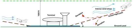
Figure 1. Intense wind shear effect on landing aircraft.

Numerous airports around the world have reaped substantial benefits from the availability of precise, high-resolution, remote sensing technologies such as the Terminal Doppler Weather Radar (TDWR) [3] and the Doppler Light Detection and Range (LiDAR) [4,5]. By a significant margin, the most prevalent methods for detecting wind shear are TDWR, ground-based anemometer networks, and wind profilers. Since the mid-1990s, this method has proved effective for alerting airports to wind shear, particularly during the passage of tropical cyclones and thunderstorms. Clear weather prevents the TDWR system from providing accurate wind data. However, certain wind-shear events are associated with airflow reaching the airport from rugged terrain. To address these circumstances, a new method of detection independent of humidity must be developed. For this purpose, the LiDAR system has been added to the TDWR as a booster in order to detect and warn of wind shear in clear skies. Doppler LiDAR can detect return signals from aerosols and provide precise Doppler wind measurements when the air is clear. Although these tracking or observation-based technological advances are effective at detecting wind shear in the vicinity of an airport, they are unable to predict when the next wind-shear event will occur, or which risk factors contribute to its occurrence [6]. Forecasting intense wind shear in the vicinity of the airport runway and the factors that contribute to the occurrence of intense wind shear are of the utmost importance, as their occurrence can cause significant challenges for departing and approaching flights.

The development of a framework for the prediction of intense wind shear requires a substantial amount of historical data on wind-shear events. Despite the fact that numerous researchers in the power and energy domain have attempted to forecast wind speed due to the demand for wind energy electricity generation and advancements in wind energy competitiveness [7,8,9], few researchers have attempted to forecast wind-shear events in the vicinity of airport runways [10,11]. For time-series modeling, several statistical and mathematical techniques have been employed in the past, such as autoregressive integrated moving average (ARIMA) [12,13,14], Kolmogorov–Zurbenko filters [15,16], exponential smoothing [17,18], and others. These often result in good forecasting accuracy. However, machine learning algorithms have recently been applied in various domains due to their high forecasting precision and improved operational efficiency [19,20,21,22,23,24]. Therefore, in this study, we propose the development of time-series prediction models of intense wind shear using machine learning algorithms. The study employed Doppler LiDAR data from 2017 to 2010 and machine learning algorithms including the Adaptive Boosting (AdaBoost) [25], Light Gradient Boosting Machine (LightGBM) [26], Categorical Boosting (CatBoost) [27], Gradient Boosting (XGBoost) [28], Random Forest [29], and Natural Gradient Boosting (NGBoost) [30] methods, optimized via a Bayesian optimization approach [31], as shown in Figure 2.

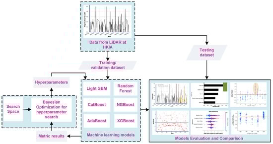
Figure 2. Framework for the time-series prediction of intense wind-shear event.

In addition to evaluating the performance of models in order to select the optimal model, crucial factors that contribute to the occurrence of intense wind shear are also revealed. Researchers in the field of civil aviation safety should seize this opportunity as understanding the complex interactions between multiple risk factors that determine the occurrence of intense wind shear is essential for aviation and meteorological applications.

2. Data and Methods

2.1. Study Location

Hong Kong International Airport (HKIA) is among the most susceptible airports in the world to the occurrence of wind-shear events, and from 1998 to 2015 a significant number of intense wind-shear events were documented. Wind-shear events occur once every 400 to 500 flights, according to HKIA-based pilot flight reports [32]. The airport is situated on Lantau Island, surrounded on three sides by open sea water and by mountains to the south that reach heights of more than 900 m above sea level. As is illustrated in Figure 3, the mountainous terrain to the south of the HKIA exacerbates wind shear by disrupting the flow of air and producing turbulence along the HKIA flight paths. Previously, HKIA had two runways: the north and south runways. However, a newly constructed runway (third runway) implies that the former north runway is now designated as the central runway. These are oriented at 070 degrees and 250 degrees. There are a total of eight possible configurations because each runway can be utilized for takeoffs and landings in either direction. For instance, runway ‘07LA’ indicates landing (‘A’ refers to arrival), with a heading angle of 070° (abbreviated to ‘07’) utilizing the left runway (hence ‘L’). This depiction demonstrates aircraft landing on the North Runway from the western side of the HKIA. Similarly, an aircraft taking off from the South Runway in the west would use runway 25LD.

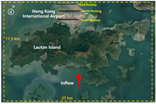
Figure 3. HKIA and surrounding terrain.

2.2. Data Processing from Doppler LiDAR

The Doppler LiDAR at the HKIA detects the magnitude and reports the location of occurrence of wind-shear events. Figure 4 depicts an illustration of a radial velocity plot obtained from a Plan Position Indicator (PPI) scan of the HKIA’s south runway LIDAR at an elevation angle of 3° from the horizon. To the west and south of the location, three nautical miles (5.6 km) west-southwest of the western end of the south runway, there was a huge area of winds in the opposite direction (colored green in Figure 4) to the dominant east–southeast airflow.

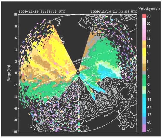
Figure 4. Wind shear detection by LIDAR.

The development of our time-series prediction models required a substantial amount of intense wind shear data for our research. Therefore, we first extracted the 2017 to 2020 wind shear data from LiDAR and filtered it to obtain only intense wind-shear events, i.e., wind shear with a magnitude greater than or equal to 30 knots. The filtration produced 3781 intense wind shear data points, which are presented in Table 1. Previous research [11] on the wind shear prediction utilized hourly data from pilot reports and weather reports, which resulted in lower accuracy due to the transient and sporadic nature of wind shear. In several instances at the HKIA, the Doppler LiDAR reported intense wind shear intervals as short as 1 min; consequently, we have considered these instances. As an example, from Table 1, we can observe that on 29 March 2019 intense wind-shear events of 37 knots and 39 knots were detected at 10:12 PM and 10:14 PM (at a 2 min interval) on runways 07CA and 07RA, respectively. The encounter locations are designated as either RWY, MD, or MF, as is shown in Figure 5. The rectangle in gray denotes the runway (RWY). On the right side of the runway, the rectangles indicate the distance in miles to the final approach (1-MF is equal to 1 nautical mile to the final approach). Likewise, the rectangles on the left indicate the distance from the runway’s departure end. For instance, 2-MD indicates two nautical miles from the runway’s edge at the departure end.

Table 1. Sample of extracted data from HKIA-based LiDAR.

Date	Time	Runway	Intense Wind Shear Magnitude	Encounter Location
16 May 2017	5:17 PM	07RA	35 knots	RWY
19 June 2017	5:19 PM	25LA	32 knots	1-MD
---	---	---	---	---
---	---	---	---	---
29 March 2019	10:12 PM	07CA	37 knots	RWY
29 March 2019	10:14 PM	07RA	39 knots	RWY
---	---	---	---	---
---	---	---	---	---
21 September 2020	3:58 AM	07RA	30 knots	2-MF

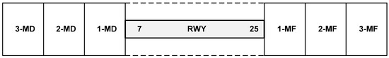
Figure 5. Schematic diagram for the representation of intense wind shear encounter locations.

2.3. Machine Learning Regression Algorithms

In this study, six machine learning regression algorithms were employed for the time-series prediction of intense wind-shear events, including LightGBM, XGBoost, NGBoost, AdaBoost, CatBoost, and RF. The fundamentals of the regression algorithm are described as follows:

2.3.1. Light Gradient Boosting Machine (LightGBM) Regression

LightGBM is a gradient learning framework that is based on decision trees and the concept of boosting. It is a variant of gradient learning. Its primary distinction from the XGBoost model is that it employs histogram-based schemes to expedite the training phase while lowering memory usage and implementing a leaf-wise expansion strategy with depth constraints. The fundamental concept of the histogram-based scheme is to partition continuous, floating-point eigenvalues into ‘k’ bins and build a histogram with a width of k. It does not require the additional storage of presorted outcomes and can also save the value after the partitioning of features, which is usually adequate to store with 8-bit integers, thereby lowering memory consumption to 1/8 of the original. This imprecise partitioning has no effect on the model’s precision. It is irrelevant whether the segmentation point is accurate or not because the decision tree is a weak study model. The regularization effect of the coarser segmentation points can also successfully prevent over-fitting.

Several hyperparameters must be adjusted for the LightGBM regression model to prevent overfitting, reduce model complexity, and achieve generalized performance. These hyperparameters are n_estimators, which is the number of boosted trees to fit, num_leaves, which is the maximum number of tree leaves for the base learners, learning_rate, which controls the estimation changes, reg_alpha, which is the L1 regularization term on weights, and reg_lambda, which is the L2 regularization term on model weights.

2.3.2. Extreme Gradient Boosting (XGBoost) Regression

XGBoost is a tree-based boosting technique variant. Fundamentally, XGBoost reveals the functional relationship, $\mathrm{\Gamma }$, between the input factors $x$ and the response $y$ via an iterative procedure wherein individual, independent trees are trained in a sequential manner on the residuals from the preceding tree. The mathematical expression for the tree-based estimates is given by Equation (1).

$$\widehat{Y}=\Gamma \left(X\right)=\frac{1}{n}{\displaystyle \sum _{k=1}^n{\Gamma }_k}\left(X\right)$$

(1)

where $\widehat{Y}$ represents the predictions and $n$ illustrates the total number of trees. The regularized objective function, $\mathsf{\Psi }\left(\mathsf{\Omega }\right)$, is minimized to learn the set of functions ${\Gamma }_k$, which are employed in the model, as shown by Equations (2) and (3).

$$\mathsf{\Psi }\left(\mathsf{\Omega }\right)={\displaystyle {\sum }_i\lambda }\left({\widehat{y}}_i,y_i\right)+{\displaystyle {\sum }_k\Pi \left({\Gamma }_k\right)}$$

(2)

$$\Pi \left({\Gamma }_k\right)=\varphi T+\frac{1}{2}l{‖\omega ‖}^2$$

(3)

where $\lambda$ represents the differentiable convex loss function that estimates the difference between the prediction and actual response. The term $\Pi$ is an additional regularization expression that panelizes the growth of further trees in the model to reduce intricacies and over-fitting. The term $\varphi$ represents the leaf’s complexity, and $T$ is the total number of leaves in a tree. Likewise, for the XGBoost regression model, hyperparameters including the n_estimators, num_leaves, learning_rate, reg_alpha, and reg_lambda must be optimized to prevent overfitting and reduce model complexity.

2.3.3. Natural Gradient Boosting (NGBoost) Regression

NGBoost is a supervised learning technique with basic probabilistic prediction capabilities. A probabilistic prediction generates a complete probability distribution over a whole outcome space, allowing users to evaluate the uncertainty in the model’s predictions. In conventional point prediction configurations, the object of concern is an estimate of the scalar function, $\mathsf{\Phi }\left(y|x\right)$, in which $x$ represents a vector of different factors and $y$ is the response, but uncertainty estimates are not considered. In a probabilistic prediction context, on the other hand, a stochastic forecast with a probability distribution, ${\mathsf{\Theta }}_{\theta }\left(y|x\right)$, is generated by predicting the parameters $\theta$. Provided that NGBoost is intended to be scalable and modular with respect to the base estimator (for instance the decision trees), probability distribution parameter (for instance, normal, Laplace, etc.), and scoring rule, NGBoost can perform probabilistic forecasts with flexible, tree-based models (for instance, the Maximum Likelihood Estimation). As is depicted in Figure 6, the input vector of the different factors $x$ in the hybrid NGBoost model is forwarded to the base estimator (decision trees) to generate a probability distribution, ${\mathsf{\Theta }}_{\theta }\left(y|x\right)$, over the a whole outcome space, $y$. The models are then improved using a scoring rule, $S\left({\mathsf{\Theta }}_{\theta },y\right)$, that produces calibrated uncertainty and point predictions using a maximum likelihood estimation function. Prior to evaluation, the NGBoost regression model parameters n_estimators and the learning_rate must be optimized.

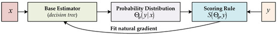
Figure 6. Mechanism of NGBoost regression algorithm.

2.3.4. Categorical Boosting (CatBoost) Regression

CatBoost is an innovative, gradient-boosting decision tree technique. It is capable of handling categorical factors and employ them in the training phase rather than in preprocessing phase. CatBoost’s advantage is that it utilizes a new pattern to determine the leaf values while choosing the tree structure, which aids in reducing over-fitting and enables the utilization of the entire training data set, i.e., it organizes the data of each instance randomly and quantifies the mean value of the instances. For the regression problem, the average of the acquired data must be utilized for a priori estimations. The parameters for the CatBoost regression model that must be optimized prior to evaluation are n_estimators, max_depth, and the learning_rate.

2.3.5. Adaptive Boosting (AdaBoost) Regression

Adaptive Boosting Regression is a straightforward ensemble learning model which creates a powerful regressor by integrating several weak learners, resulting in a high-accuracy model. The core concept is to establish the weights of weak regressors and train the dataset at each iteration such that reliable projections of unusual observations may be made. The working principle of AdaBoost is provided below:

• The weight distribution $\left(\pi \right)$ is initialized as $\pi =1/m$;
• At iteration $t$, the weak learning is trained, i.e.,${\mathrm{h}}_t: x\to \Re$, using the weight distribution;
• The weight distribution is updated in accordance with previous instances of the training dataset as ${\pi }_k=\frac{{\pi }_{k-1}{\mathit{exp}}^{-{\psi }_{k}h\left(x_k\right)}}{\Omega }$;
• The final output over all the iterations $t=1,2,\dots ,T$ is returned as $f\left(X\right)={\displaystyle {\sum }_{t\mathit{=}\mathit{1}}^T{\pi }_t{h}_t\left(X\right)}$ and $H\left(X\right)=\mathit{sign}\left(f\left(X\right)\right)$.

The AdaBoost model uses a decision stump as a weak learner. The critical hyperparameters that need to be tuned during the learning process are the n_estimators and learning_rate. The n_estimators are the number of decision stump to train iteratively and the learning_rate controls the contribution of each learner. There is required to be a trade-off between both the n_estimators and learning_rate.

2.3.6. Random Forest (RF) Regression

The RF is an ensemble of tree-based predictors in which each tree is trained with values of an independently sampled random vector that has the same distribution for all other trees in the forest. The $k^{th}$ tree is conceptually trained using an independent random vector, ${\zeta }_k$, with the same distribution as previous random vectors, ${\zeta }_{k-1}$, resulting in a tree, $\psi \left({\rm X},{\zeta }_k\right)$, in which $X$ is the input vector of different factors. When a large number of trees are grown in a forest, their mean predictions are obtained, which improves the accuracy of predictions and prevents over-fitting. Mathematically, it can be illustrated as Equation (4).

$$\widehat{Y}=\frac{1}{l}{\displaystyle \sum _{k=1}^l{\psi }_k\left(X\right)}$$

(4)

where $\widehat{Y}$ represent the response and $l$ is the total amount of generated trees $\left(1\le k\le l\right)$. The mean squared generalization error of any tree $\psi \left({\rm X}\right)$ is illustrated as $E_{{\rm X},Y}{\left(Y-\psi \left({\rm X}\right)\right)}^2$ for the input vector of difference $\left(X\right)$ and the response vector $\left(Y\right)$. As the number of trees in the forest approaches the infinity, the mean squared generalization almost certainly becomes:

$$E_{{\rm X},Y}{\left(Y-{\Lambda }_k\psi \left(X,{\zeta }_k\right)\right)}^2\to E_{{\rm X},Y}{\left(Y-E_{\zeta }\psi \left(X,\zeta \right)\right)}^2$$

(5)

A few crucial hyperparameters must be tuned during the learning phase in order to achieve an optimized prediction score for the RF model. These hyperparameters are the n_estimators, which is the number of trees in the forest, and the max_depth, which is the maximum number of levels, or branches between the root node and the deepest leaf node.

2.4. Principle of Bayesian Optimization

The structure parameters of a machine learning model are its hyperparameters. Adapting a machine learning model to multiple situations requires adjusting the hyperparameters [33,34]. In this study, a Bayesian hyperparameter optimization method is implemented. The goal is to establish the mapping, $f\left(x,\theta \right)$, in which $y$ is the response, $x$ is the input vector, and the $\theta$ vector determines the size of the mapping. The core principle of Bayesian optimization is adjusting the hyperparameter of a given model in order to formulate a model of the loss function. It utilizes a loss function to efficiently search for and select the optimal set of hyperparameters. Employing the hyperparameter $\theta$ in a tree-based machine learning model as one of the points in the multidimensional search space for the optimization, the hyperparameter that minimizes the loss function value, $f\left(\theta \right)$, can be found in the set $A\in X^d$, as shown by Equation (6).

$${\theta }^{*}=\arg \underset{\theta \in A}{\min }f\left(\theta \right)$$

(6)

Usually, there is no prior information about the model’s structure; therefore, it is assumed that the noise in the observation is shown by Equation (7).

$$y\left(\theta \right)=f\left(\theta \right)+\epsilon , \mathrm{and} \epsilon ~N\left(0,{\sigma }_{noise}^2\right)$$

(7)

The Bayesian framework offers two fundamental options. First, a hypothesis function. $\mathit{p}\left(f|\mathcal{D}\right)$ (also known as a prior function). must be chosen to represent the hypothesis of the function to be optimized. Second, the posterior model determines the acquisition function for determining the subsequent test point. Using the prior function,$\mathit{p}\left(f|\mathcal{D}\right)$, the Bayesian framework constructs a loss function model based on an observed data sample, $\mathcal{D}$. The prior function model, $\mathit{p}\left(f|\mathcal{D}\right)$, chooses between optimization and development based on its characteristics.

2.5. Performance Assessment

The generalization capacity of various machine learning regression models could be synthetically quantified using four different metrics: the mean absolute error (MAE), mean squared error (MSE), root mean squared error (RMSE), and the R-square (R², coefficient of determination). According to Equation (8), the MAE is the average of the individual prediction errors’ absolute values across all instances. The average squared difference between observed and predicted values, as shown in Equation (9) is how the MSE computes regression model error. According to Equation (10), the RMSE is the square root of the difference between the observed and predicted values. A regression model’s ability to accurately predict values is indicated by R², which ranges from 0 to 1. R² is provided by Equation (11).

$$\mathrm{MAE}={\displaystyle {\sum }_{\chi =1}^{\Phi }\frac{\left|y_{\chi }-{\widehat{y}}_{\chi }\right|}{\chi }}$$

(8)

$$\mathrm{MSE}=\frac{1}{\chi }{{\displaystyle {\sum }_{\chi =1}^{\Phi }\left(y_{\chi }-{\widehat{y}}_{\chi }\right)}}^2$$

(9)

$$\mathrm{RMSE}=\sqrt{{\displaystyle {\sum }_{\chi =1}^{\Phi }\frac{{\left(y_{\chi }-{\widehat{y}}_{\chi }\right)}^2}{\chi }}}$$

(10)

$$R^2=1-\frac{{\displaystyle {\sum }_{x=1}^{\Phi }{\left(y_{\chi }-{\widehat{y}}_{\chi }\right)}^2}}{{\displaystyle {\sum }_{\chi =1}^{\Phi }{\left(y_{\chi }-y_{avg}\right)}^2}}$$

(11)

where $\chi$ is the total number of observations, $y$ represents the actual observation value, and $\widehat{y}$ represents the predicted value.

3. Results and Discussion

The LiDAR data of 2017 to 2020 from the Hong Kong Observatory and the aviation weather forecast department at HKIA were used to train and test six different machine learning regression models with the goal of determining how well these models can predict the occurrence of intense wind-shear events. Figure 7a depicts the total LiDAR-obtained intense wind-shear data from 1 January 2017 to 31 December 2020. The data from 1 January 2017 to 31 December 2019 are the training set, which is depicted by the black line in Figure 7b, while the data from 1 January 2020 to 31 December 2020 are the test set, which is depicted by the green line. The vertical red line with dashes divides the training data from the test data.

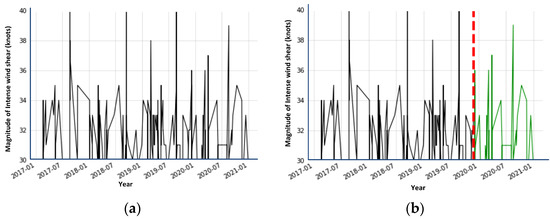
Figure 7. LiDAR data: (a) 2017–2020 intense wind shear data; (b) splitting data into train and test sets.

The statistical information of the intense wind shear dataset is shown in Table 2. The machine learning models, coupled with Bayesian optimization and a 5-fold cross validation, provide the predicted results based on the optimal hyperparameters. The Hyperopt python package was used for the implementation of Bayesian optimization. The optimal hyperparameters with search space are shown in Table 3. Table 4 shows the comparison of the prediction performance of the machine learning regression algorithms. The predicted intense wind shear values, based the on machine learning regression algorithms, are plotted in Figure 8, and the residual errors by the machine learning models are shown by the scatter plots (Figure 9). In addition, feature importance and contribution are illustrated by Figure 10, and the effect of important factors is shown by Figure 11.

Table 2. Statistical information of intense wind shear from HKIA-based LIDAR.

Dataset	Max	Median	Min	Mean	St. Dev
Entire dataset	40	33	30	33.881	2.596
Train dataset	40	33	30	33.743	2.455
Test dataset	40	34	30	33.921	2.366

Table 3. Optimal hyperparameters of machine learning regression algorithms.

Algorithm	Hyperparameters	Range	Optimal Values
LightGBM	{(n_estimators), (num_leaves), (learning rate), (reg_lambda), (reg_alpha)}	{(100–1500), (30–100), (0.001–0.2), (1.1–1.5), (1.1–1.5)}	{1180, 28, 0.10, 1.19, 1.01}
CatBoost	{(n_estimators), (max_depth), (learning rate)}	{(200–1500), (2–15), (0.001–0.2)}	{1060, 8, 0.08}
AdaBoost	{(n_estimators), (learning rate)}	{(100–1500), (0.001–0.2)}	{790, 0.04}
RF	{(n_estimators), (max_depth)}	{(50–1000), (2–15)}	{955, 5}
XGBoost	{(n_estimators), (num_leaves), (learning rate), (reg_lambda), (reg_alpha)}	{(100–1500), (30–100), (0.001–0.2), (1.1–1.5), (1.1–1.5)}	{880, 65, 0.05, 1.18, 1.40}
NGBoost	{(n_estimators), (learning rate)}	{(100–1500), (0.001–0.2)}	{1130, 0.03}

Table 4. Performance assessment of Bayesian optimized machine learning models.

Models	Performance Metrics
	MAE	MSE	RMSE	R-Square
LightGBM	1.813	5.840	2.416	0.711
NGBoost	1.858	6.298	2.509	0.619
Random Forest	1.851	6.194	2.488	0.647
CatBoost	1.795	5.783	2.404	0.753
XGBoost	1.764	5.611	2.368	0.859
AdaBoost	1.863	6.815	2.610	0.549

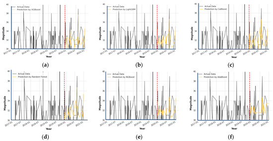
Figure 8. Predictions using machine learning models: (a) prediction of intense wind shear by XGBoost; (b) prediction of intense wind shear by LightGBM; (c) prediction of intense wind shear by CatBoost; (d) prediction of intense wind shear by Random Forest; (e) prediction of intense wind shear by NGBoost; and (f) prediction of intense wind shear by AdaBoost.

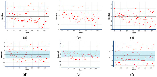
Figure 9. Residual analysis by machine learning regression models; (a) NGBoost; (b) LightGBM; (c) CatBoost; (d) Random Forest; (e) XGBoost; and (f) AdaBoost.

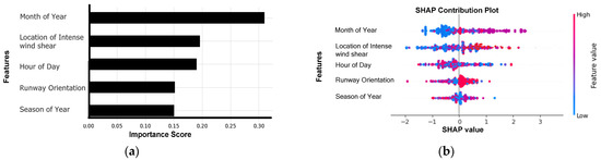
Figure 10. Importance and contribution plots: (a) XGBoost-based feature importance plot and (b) XGBoost-based SHAP contribution plot.

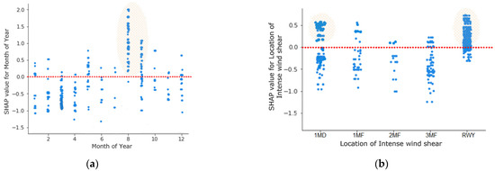
Figure 11. Effect of factors on the Intense wind shear: (a) month of year and (b) encounter location of intense wind shear.

Table 4 demonstrates that the Bayesian optimized-XGBoost model outperforms other machine learning models with a minimum MAE value of 1.764, an MSE value of 5.611, an RMSE value of 2.368, and a maximum R-square value of 0.859. The AdaBoost model, with an MAE of 1.863, MSE of 6.815, RMSE of 2.610, and an R-square value of 0.549, performs the worst. In addition, an analysis of Figure 8 reveals that XGBoost appears to provide a better fit of the actual test intense wind shear time-series and a smaller residual error, represented by red dots closer to horizontal line, when compared to other forecasting results (Figure 9).

The importance and contribution of the factors are depicted in Figure 10 and are based on the importance score that was determined by the Bayesian optimized-XGBoost model and the XGBoost-based SHAP contribution plot, respectively. In both cases, it was observed that the month of year was the most significant feature, with an importance score of 0.33, followed by the location of intense wind shear (0.19), the hour of the day (0.18), and runway orientation (0.16). Figure 10b revealed that months of the year coded by lower values are less likely to cause intense wind shear, in contrast to those with medium values. Similarly, the location of an encounter with intense wind shear, represented by higher values, is more likely to cause intense wind shear. In the following section, each important feature that plays a role in the occurrence of intense wind shear is discussed in more detail.

Figure 11a,b depict the scatter plot of two significant factors. Figure 11a illustrates that the highest number of intense wind-shear events were recorded in August. The intense wind shear in August might be due to cross-mountain airflow, which occurs over the HKIA in August and September, during the south-west monsoon, or during passages of tropical cyclones. These terrain-disrupted airflows cause a number of intense wind-shear events, which negatively impact HKIA’s flight safety and operations. This is also consistent with the previous study [11,35].

On the RWY and 1-MD from the edge of the RWY, a large number of intense wind-shear events are observed, as shown in Figure 11b. A small number of intense wind-shear events were observed as the distance increases from the RWY. To the best of our knowledge, none of the previous studies have pinpointed the location where intense wind shear is most prevalent. Nevertheless, our research indicates that RWY and 1-MD from edge of RWY are crucial to the occurrence of intense wind shear. Pilots must maintain vigilance at 1-MD during takeoff.

4. Conclusions and Recommendations

This study is a first attempt at developing a time-series prediction model of intense wind-shear events based on HKIA-based LiDAR data. Six state-of-the-art machine learning regression algorithms, optimized via the Bayesian optimization approach, were employed in this regard. The HKIA-based LiDAR data from 2017 to 2020 was used as the input. From this study, the following conclusions can be drawn:

• On the testing dataset (intense wind-shear data of HKIA-based LiDAR from 1 January 2020 to 31 December 2020), the Bayesian optimized-XGBoost model had the best overall performance of all the optimized machine learning regression models, with an MAE (1.764), MSE (5.611), RMSE (2.368), and R-square (0.859), which was followed by Bayesian optimized-CatBoost model, which had an MAE (1.795), MSE (5.783), RMSE (2.404), and R-square (0.753);
• The AdaBoost regression model demonstrated the lowest performance in terms of MAE (1.863), MSE (6.815), RMSE (2.610), and R-square (0.549);
• The Bayesian optimized-XGBoost model demonstrated that the month of year was the most influential factor, followed by distance of occurrence of intense wind shear from the RWY;
• August is more likely to have intense wind-shear events. Similarly, most of the intense wind-shear events are expected to occur at RWY and 1-MD from the runway departure end. The pilots are required to be cautious during takeoff.

For aviation authorities and researchers interested in aviation safety, the methodology put forth in this study can be used to conduct an extensive investigation of intense wind shear. The study covered in this paper was the time-series prediction of intense wind shear using six machine learning models coupled with a Bayesian optimization approach. Future research might use an amalgamation of a stacking ensemble and various other machine learning ensemble algorithms with a number of additional risk factors, such as the impact of atmospheric pressure and temperature. In addition, the causes of the occurrence of wind shear (weather- or terrain-induced) could be used in future research.

References

- Chan, P.W. Severe wind shear at Hong Kong International airport: Climatology and case studies. Meteorol. Appl. 2017, 3, 397–403. [Google Scholar] [CrossRef]
- Bretschneider, L.; Hankers, R.; Schönhals, S.; Heimann, J.M.; Lampert, A. Wind Shear of Low-Level Jets and Their Influence on Manned and Unmanned Fixed-Wing Aircraft during Landing Approach. Atmosphere 2021, 13, 35. [Google Scholar] [CrossRef]
- Michelson, M.; Shrader, W.; Wieler, J. Terminal Doppler weather radar. Microw. J. 1990, 33, 139. [Google Scholar]
- Shun, C.; Chan, P. Applications of an infrared Doppler lidar in detection of wind shear. J. Atmos. Ocean. Technol. 2008, 25, 637–655. [Google Scholar] [CrossRef]
- Li, L.; Shao, A.; Zhang, K.; Ding, N.; Chan, P.-W. Low-level wind shear characteristics and LiDAR-based alerting at Lanzhou Zhongchuan International Airport, China . J. Meteorol. Res. 2020, 34, 633–645. [Google Scholar] [CrossRef]
- Hon, K.-K. Predicting low-level wind shear using 200-m-resolution NWP at the Hong Kong International Airport. J. Appl. Meteorol. Climatol. 2020, 59, 193–206. [Google Scholar] [CrossRef]
- Zhang, Y.; Pan, G.; Chen, B.; Han, J.; Zhao, Y.; Zhang, C. Short-term wind speed prediction model based on GA-ANN improved by VMD. Renew. Energy 2020, 156, 1373–1388. [Google Scholar] [CrossRef]
- Zhang, Z.; Ye, L.; Qin, H.; Liu, Y.; Wang, C.; Yu, X.; Yin, X.; Li, J. Wind speed prediction method using shared weight long short-term memory network and Gaussian process regression. Appl. Energy 2019, 247, 270–284. [Google Scholar]
- Cai, H.; Jia, X.; Feng, J.; Li, W.; Hsu, Y.M.; Lee, J. Gaussian Process Regression for numerical wind speed prediction enhancement. Renew. Energy 2020, 146, 2112–2123. [Google Scholar] [CrossRef]
- Khattak, A.; Chan, P.W.; Chen, F.; Peng, H. Prediction and Interpretation of Low-Level Wind Shear Criticality Based on Its Altitude above Runway Level: Application of Bayesian Optimization–Ensemble Learning Classifiers and SHapley Additive explanations. Atmosphere 2022, 12, 2102. [Google Scholar] [CrossRef]
- Chen, F.; Peng, H.; Chan, P.W.; Ma, X.; Zeng, X. Assessing the risk of windshear occurrence at HKIA using rare-event logistic regression. Meteorol. Appl. 2020, 27, e1962. [Google Scholar] [CrossRef]
- Singh, R.K.; Rani, M.; Bhagavathula, A.S.; Sah, R.; Rodriguez-Morales, A.J.; Kalita, H.; Nanda, C.; Sharma, S.; Sharma, Y.D.; Rabaan, A.A.; et al. Prediction of the COVID-19 pandemic for the top 15 affected countries: Advanced autoregressive integrated moving average (ARIMA) model. JMIR Public Health Surveill. 2020, 6, e19115. [Google Scholar] [CrossRef] [PubMed]
- Singh, S.; Parmar, K.S.; Kumar, J.; Makkhan, S.J. Development of new hybrid model of discrete wavelet decomposition and autoregressive integrated moving average (ARIMA) models in application to one month forecast the casualties cases of COVID-19. Chaos Solitons Fractals 2020, 135, 109866. [Google Scholar] [CrossRef] [PubMed]
- Dansana, D.; Kumar, R.; Das Adhikari, J.; Mohapatra, M.; Sharma, R.; Priyadarshini, I.; Le, D.N. Global forecasting confirmed and fatal cases of COVID-19 outbreak using autoregressive integrated moving average model. Front. Public Health 2020, 8, 580327. [Google Scholar] [CrossRef] [PubMed]
- Plitnick, T.A.; Marsellos, A.E.; Tsakiri, K.G. Time series regression for forecasting flood events in Schenectady, New York. Geosciences 2018, 8, 317. [Google Scholar] [CrossRef]
- Sadeghi, B.; Ghahremanloo, M.; Mousavinezhad, S.; Lops, Y.; Pouyaei, A.; Choi, Y. Contributions of meteorology to ozone variations: Application of deep learning and the Kolmogorov-Zurbenko filter. Environ. Pollut. 2022, 310, 119863. [Google Scholar] [CrossRef]
- Smyl, S. A hybrid method of exponential smoothing and recurrent neural networks for time series forecasting. Int. J. Forecast. 2020, 36, 75–85. [Google Scholar] [CrossRef]
- Sinaga, H.; Irawati, N. A medical disposable supply demand forecasting by moving average and exponential smoothing method. In Proceedings of the 2nd Workshop on Multidisciplinary and Applications (WMA) 2018, Padang, Indonesia, 24–25 January 2018. [Google Scholar]
- Zhang, S.; Khattak, A.; Matara, C.M.; Hussain, A.; Farooq, A. Hybrid feature selection-based machine learning Classification system for the prediction of injury severity in single and multiple-vehicle accidents. PLoS ONE 2022, 17, e0262941. [Google Scholar] [CrossRef]
- Dong, S.; Khattak, A.; Ullah, I.; Zhou, J.; Hussain, A. Predicting and analyzing road traffic injury severity using boosting-based ensemble learning models with SHAPley Additive exPlanations. Int. J. Environ. Res. Public Health 2022, 19, 2925. [Google Scholar] [CrossRef]
- Khattak, A.; Almujibah, H.; Elamary, A.; Matara, C.M. Interpretable Dynamic Ensemble Selection Approach for the Prediction of Road Traffic Injury Severity: A Case Study of Pakistan’s National Highway N-5. Sustainability 2022, 14, 12340. [Google Scholar] [CrossRef]
- Goodman, S.N.; Goel, S.; Cullen, M.R. Machine learning, health disparities, and causal reasoning. Ann. Intern. Med. 2018, 169, 883–884. [Google Scholar] [CrossRef]
- Guo, R.; Fu, D.; Sollazzo, G. An ensemble learning model for asphalt pavement performance prediction based on gradient boosting decision tree. Int. J. Pavement Eng. 2022, 23, 3633–3644. [Google Scholar] [CrossRef]
- Zhao, Y.; Deng, W. Prediction in Traffic Accident Duration Based on Heterogeneous Ensemble Learning. Appl. Artif. Intell. 2022, 36, 2018643. [Google Scholar] [CrossRef]
- Freund, Y.; Schapire, R.; Abe, N. A short introduction to boosting. J. Jpn. Soc. Artif. Intell. 1999, 14, 1612. [Google Scholar]
- Ke, G.; Meng, Q.; Finley, T.; Wang, T.; Chen, W.; Ma, W.; Ye, Q.; Liu, T.Y. Lightgbm: A highly efficient gradient boosting decision tree. Adv. Neural Inf. Process. Syst. 2017, 30, 52. [Google Scholar]
- Prokhorenkova, L.; Gusev, G.; Vorobev, A.; Dorogush, A.V.; Gulin, A. CatBoost: Unbiased boosting with categorical features. Adv. Neural Inf. Process. Syst. 2018, 31. [Google Scholar]
- Chen, T.; Guestrin, C. Xgboost: A scalable tree boosting system. In Proceedings of the 22nd Acm Sigkdd International Conference on Knowledge Discovery and Data Mining, San Francisco, CA, USA, 13–17 August 2016; pp. 785–794. [Google Scholar]
- Breiman, L. Random forests. Mach. Learn. 2001, 45, 5–32. [Google Scholar] [CrossRef]
- Duan, T.; Anand, A.; Ding, D.Y.; Thai, K.K.; Basu, S.; Ng, A.; Schuler, A. Ngboost: Natural gradient boosting for probabilistic prediction. In Proceedings of the 37th International Conference on Machine Learning, Virtual Event, 13–18 July 2020; pp. 2690–2700. [Google Scholar]
- Snoek, J.; Larochelle, H.; Adams, R.P. Practical Bayesian optimization of machine learning algorithms. In Advances in Neural Information Processing Systems 25 (NIPS 2012); 2012; Volume 25, Available online: https://proceedings.neurips.cc/paper/2012/hash/05311655a15b75fab86956663e1819cd-Abstract.html (accessed on 4 August 2022).
- Chan, P.; Hon, K. Observation and numerical simulation of terrain-induced windshear at the Hong Kong International Airport in a planetary boundary layer without temperature inversions. Adv. Meteorol. 2016, 2016, 1454513. [Google Scholar] [CrossRef]
- Wu, J.; Chen, X.Y.; Zhang, H.; Xiong, L.D.; Lei, H.; Deng, S.H. Hyperparameter optimization for machine learning models based on Bayesian optimization. J. Electron. Sci. Technol. 2019, 17, 26–40. [Google Scholar]
- Victoria, A.H.; Maragatham, G. Automatic tuning of hyperparameters using Bayesian optimization. Evol. Syst. 2021, 12, 217–223. [Google Scholar] [CrossRef]
- Chan, P.W.; Hon, K.K. Observations and numerical simulations of sea breezes at Hong Kong International Airport. Weather 2022, 78, 55–63. [Google Scholar] [CrossRef]
Disclaimer/Publisher’s Note: The statements, opinions and data contained in all publications are solely those of the individual author(s) and contributor(s) and not of MDPI and/or the editor(s). MDPI and/or the editor(s) disclaim responsibility for any injury to people or property resulting from any ideas, methods, instructions or products referred to in the content. |
© 2023 by the authors. Licensee MDPI, Basel, Switzerland. This article is an open access article distributed under the terms and conditions of the Creative Commons Attribution (CC BY) license (https://creativecommons.org/licenses/by/4.0/).